Article

Physics-Informed Deep Learning for Traffic State Estimation: A Survey and the Outlook

1
Department of Civil Engineering and Engineering Mechanics, Columbia University, New York, NY 10027, USA
2
Data Science Institute, Columbia University, New York, NY 10027, USA
*
Author to whom correspondence should be addressed.
These authors contributed equally to this work.
Algorithms 2023, 16(6), 305; https://doi.org/10.3390/a16060305
Submission received: 23 May 2023 / Revised: 13 June 2023 / Accepted: 14 June 2023 / Published: 17 June 2023

Abstract

:
For its robust predictive power (compared to pure physics-based models) and sample-efficient training (compared to pure deep learning models), physics-informed deep learning (PIDL), a paradigm hybridizing physics-based models and deep neural networks (DNNs), has been booming in science and engineering fields. One key challenge of applying PIDL to various domains and problems lies in the design of a computational graph that integrates physics and DNNs. In other words, how the physics is encoded into DNNs and how the physics and data components are represented. In this paper, we offer an overview of a variety of architecture designs of PIDL computational graphs and how these structures are customized to traffic state estimation (TSE), a central problem in transportation engineering. When observation data, problem type, and goal vary, we demonstrate potential architectures of PIDL computational graphs and compare these variants using the same real-world dataset.

1. Introduction

Physics-informed deep learning (PIDL) [1], also named “theory-guided data science” [2], “model-informed machine learning” [3], or “physics-informed machine learning” [4], has gained increasing traction in various scientific and engineering fields. Its underlying rationale is to leverage the pros of both physics-based and data-driven approaches while compensating the cons of each. A physics-based approach refers to using scientific hypotheses of what underlying physics govern observations, e.g., first principles. Normally, scientists or engineers first come up with a prior assumption of how a quantity of interest is computed from other physics quantities. Then, laboratory or field experiments are designed to collect data that are used to calibrate the involved parameters. In contrast, a data-driven approach does not bear any prior knowledge of how things work and how different quantities are correlated. Instead, it relies on machine learning (ML) techniques, such as deep learning (DL), to learn and infer patterns from data. The former is data-efficient and interpretable but may not be generalizable to unobserved data, while the latter is generalizable at the cost of relying on huge amounts of training samples and may be incapable of offering deductive insights. Thus, the PIDL paradigm opens up a promising research direction that leverages the strengths of both physics-based and data-driven approaches. Figure 1 summarizes the amounts of data (in x-axis) and scientific theory (in y-axis) used for each paradigm. Model-based approaches heavily rely on scientific theory discovered from the domain knowledge and use little data for system discovery, while machine learning approaches mostly rely on data for mechanism discovery, In contrast, PIDL employs a small amount of data (i.e., “small data” [4]) for pattern discovery while leveraging a certain amount of scientific knowledge to impose physically consistent constraints. The “sweetspot” of PIDL lies in the small data and partial knowledge regime. In other words, PIDL achieves the best performance in accuracy and robustness with small data and partial domain knowledge. In this paper, we will validate the advantage of PIDL using transportation applications, and present a series of experiments using the same real-world dataset against conventional physics-based models.

1.1. Scope of This Survey

There are a variety of structure designs for PIDL. Here, we primarily focus on the PIDL framework that is represented by a hybrid computational graph (HCG) consisting of two graphs: a physics-informed computational graph (PICG) and a physics-uninformed neural network (PUNN). Despite numerous benefits of PIDL, there are still many open questions that need to be answered, including the construction of the HCG, the choice of the physics and the architecture of the PICG, the architecture of the PUNN, the loss function, and the training algorithms. Among them, how to encode the physics into (deep) neural networks (DNNs) remains under-explored and varies case by case and across domains. In this paper, we will primarily establish a systematic design pipeline for hybrid computational graphs that would facilitate the integration of physics and DL. To this end, we will review the state-of-the-art of the PIDL architecture in the traffic state estimation (TSE) problem. This survey paper can be used as a guideline for researchers at large when they consider using PIDL for problems at hand.
We have seen a growing number of studies that apply PIDL to physical and biological systems [4,5]. However, its feasibility for social systems, in particular, human decision-making processes, such as driving behaviors, remains largely unexploited. Humans’ decision making involves complex cognitive processes compounded by perception errors, noisy observations, and output randomness. Moreover, human driving behaviors exhibit highly unstable and nonlinear patterns, leading to stop-and-go traffic waves and traffic congestion [6,7,8]. Accordingly, neither model-driven nor data-driven approaches alone suffice to predict such behaviors with high accuracy and robustness. Therefore, we strongly believe that a hybrid method, which leverages the advantages of both model-driven and data-driven approaches, is promising [9,10].
There is a vast amount of literature on TSE [11,12] and on PIDL [4,5]. To distinguish this work from other survey papers in TSE, here, we primarily focus on data-driven approaches, PIDL in particular. Since PIDL for TSE is less studied than physics-based models, and the existing literature is focused on single roads, we will primarily examine TSE along links, and leave TSE on a road network which includes both link and node models for future research. To distinguish this work from other PIDL surveys, we primarily focus on the modular design of the hybrid PIDL paradigm and show how to customize various designs for accurate and robust identification of traffic dynamic patterns. Here, the modular design refers to the architecture design of each component in the graph and how these components are wired, in other words, how physics laws are injected into DNNs. The generic architecture of a PIDL consists of two computational graphs: one is a DNN (i.e., the data-driven component) for predicting the unknown solution, while the other is a computational graph (i.e., the physics-driven component, also called “physics-informed neural networks (PINNs)” in [1]), in which physics is represented, for evaluating whether the prediction aligns with the given physics. The physics encoded computational graph can be treated as a regularization term of the other deep neural network to prevent overfitting, i.e., high-variance. In summary, the hybrid of both components overcomes high-bias and high-variance induced by each individual one, rendering it possible to leverage the advantage of both the physics-based and data-driven methods in terms of model accuracy and data efficiency.

1.2. Contributions

The application of PIDL to TSE is a relatively new area. We hope that the insights in this work into the modular design of the hybrid PIDL paradigm, as well as the established visualization tool, will not only be useful to guide transportation researchers to pursue PIDL, but also facilitate researchers at large to better understand a PIDL pipeline when applied to their own application domains.
Overall, this paper offers a comprehensive overview of the state-of-the-art in TSE using PIDL, while striving to provide insights into the pipeline of implementing PIDL, from architecture design to training and testing. In particular, the contributions of this work are:
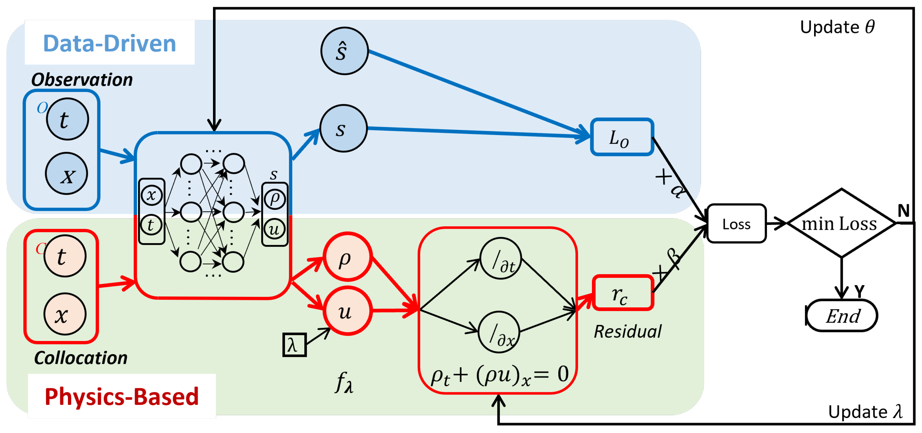
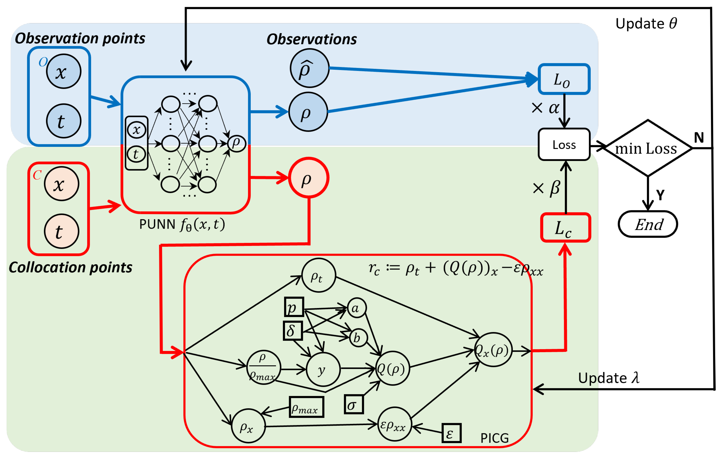
  • propose a computational graph that visualizes both physics and data components in PIDL;
  • establish a generic way of designing each module of the PIDL computational graphs for both predication and uncertainty quantification;
  • benchmark the performance of various PIDL models using the same real-world dataset and identify the advantage of PIDL in the “small data” regime.
The rest of the paper is organized as follows: Section 2 introduces the preliminaries of TSE and the state of the art. Section 3.1 lays out the framework of PIDL for TSE. Two types of problems for TSE, namely, deterministic prediction and uncertainty quantification, are detailed in Section 3 and Section 4, respectively. Section 5 concludes our work and projects future research directions in this promising arena.

2. Preliminaries and Related Work

2.1. PIDL

Definition 1. 
Generic framework for physics-informed deep learning. Define location x [ 0 , L ] and time t [ 0 , T ] and L , T R + . Then, the spatiotemporal (ST) domain of interest is a continuous set of points: D = { ( x , t ) | x [ 0 , L ] , t [ 0 , T ] } . Denote the state as s and its observed quantity as s ^ . Denote the (labeled) observation O , B , I and the (unlabeled) collocation points C below:
O = { ( x ( i ) , t ( i ) ; s ^ ( i ) ) } i = 1 N o : within domain observation , B = { t ( i b ) ; s ^ ( i b ) } i b = 1 N b : boundary observation , I = { x ( i 0 ) ; s ^ ( i 0 ) } i 0 = 1 N 0 : initial observation , C = { ( x ( j ) , t ( j ) ) } j = 1 N c : collocation points ,
where i and j are the indices of the observation and collocation points, respectively. i b , i 0 are the indices of the boundary and initial data, respectively. The number of observed data, boundary and initial conditions, and collocation states are denoted as N o , N b , N 0 , N c , respectively. The subscripts b , 0 represent the boundary and initial condition indices, respectively.
We design a hybrid computational graph (HCG) consisting of two computational graphs: (1) a PUNN, denoted as f θ ( x , t ) , to approximate mapping s ( i ) , and (2) a PICG, denoted as f λ ( x , t ) , for computing traffic states of s ( j ) from collocation points. In summary, a general PIDL model, denoted as f θ , λ ( x , t ) , is to train an optimal parameter set θ for PUNN and an optimal parameter set λ for the physics. The PUNN parameterized by the solution θ can then be used to predict a traffic state s ^ n e w on a new set of observed ST points O n e w D , and λ is the most likely model parameters that describe the intrinsic physics of the observed data.
One important application of PIDL is to solve generic partial differential equations (PDE). We will briefly introduce the underlying rationale. Define a PDE over the ST domain as:
s t ( x , t ) + N x [ s ( x , t ) ] = 0 , ( x , t ) D , B [ s ( x , t ) ] = 0 , ( x , t ) D , I [ s ( x , 0 ) ] = 0 ,
where N x ( · ) is the nonlinear differential operator, B , I are the boundary and initial condition operators, respectively, D = { ( 0 , t ) | t [ 0 , T ] } { ( L , t ) | t [ 0 , T ] } is the set of ST points on the boundary of the domain D , and s ( x , t ) is the exact solution of the PDE. Now, we will approximate the PDE solution, s ( x , t ) , by a DNN parametrized by θ , f θ ( x , t ) , which is PUNN. If this PUNN is exactly equivalent to the PDE solution, then we have
f θ ( x , t ) + N x [ f θ ( x , t ) ] = 0 , ( x , t ) D .
Otherwise, we define a residual function r c ( x , t ) = [ f θ ( x , t ) ] t + N x [ f θ ( x , t ) ] . If PUNN is well trained, the residual needs to be as close to zero as possible. Figure 2 describes the schematic of using PUNN to approximate PDE solutions.
The physics is usually encoded as governing equations, physical constrains, or regularity terms in loss functions when training PUNNs [13]. When “soft regularization” was implemented by [14], the loss in PIDL was a weighted sum of two distance measures: one for the distance between the observed action and predicted one (also known as data discrepancy) and the other for the distance between the computed action from the physics and the predicted one (also known as physics discrepancy). Its specific forms will be detailed in Section 3 and Section 4.

2.2. Traffic State Estimation

Traffic state inference is a central problem in transportation engineering and serves as the foundation for traffic operation and management.
Definition 2. 
Traffic state estimation (TSE) infers traffic states in single lane or multiple lanes along a stretch of highway or arterial segments over a period of time, represented by traffic density (veh/km/lane, denoted by ρ), traffic velocity (km/lane/hour, denoted by u), and traffic flux or volume (veh/lane/hour, denoted by q) using noisy observations from sparse traffic sensors [12]. The ultimate goal of TSE is traffic management and control, building on the inferred traffic states.
Remark 1. 
  • These three traffic quantities are connected via a universal formula:
    q = ρ u .
    Knowing two of these quantities automatically derives the other. Thus, in this paper, we will primarily focus on ρ , u , and q can be derived using Equation (4).
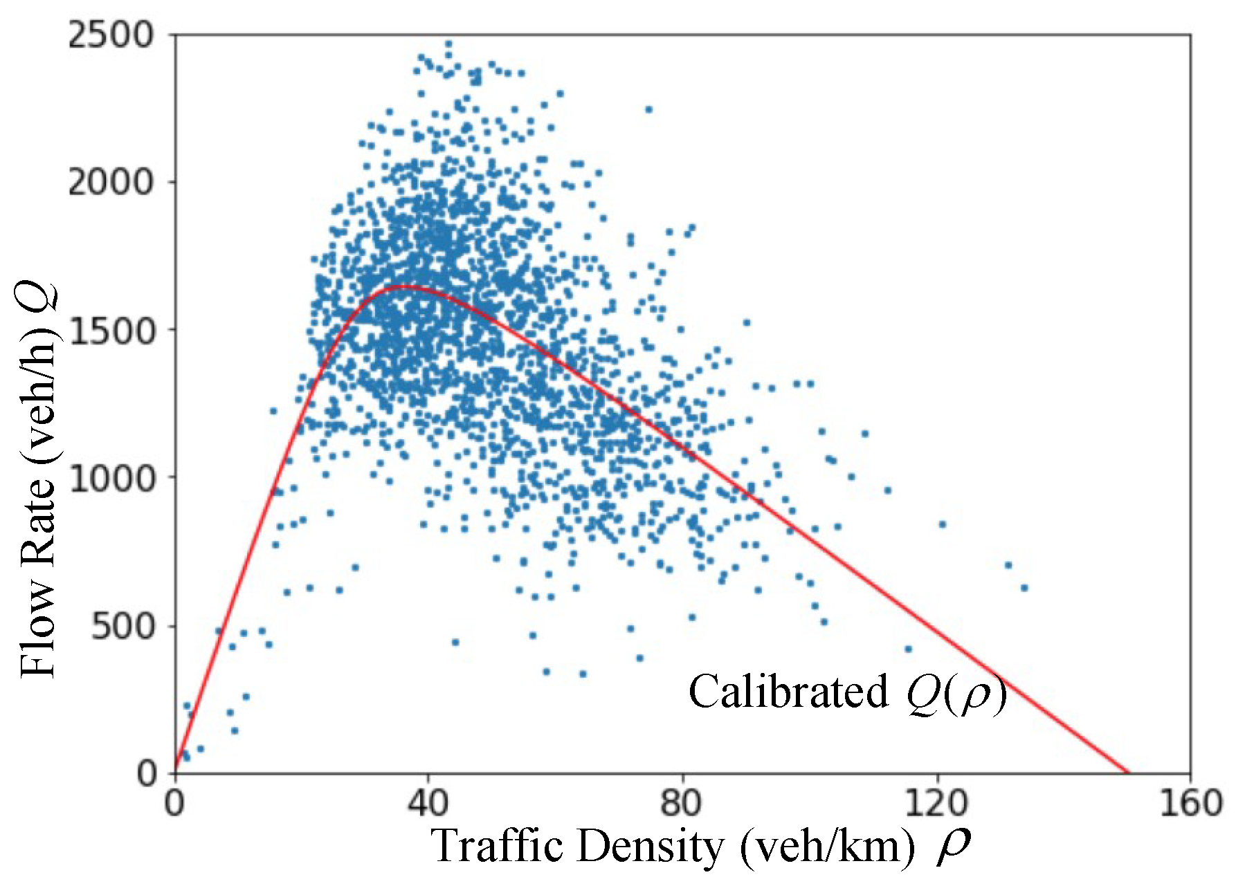
  • q [ 0 , q m a x ] , ρ [ 0 , ρ j a m ] , u [ 0 , u m a x ] , where q m a x is the capacity of a road, ρ j a m is the jam density (i.e., the bumper-to-bumper traffic scenario), and u m a x is the maximum speed (and usually represented by a speed limit). How to calibrate these parameters is shown in Table 1.
TSE is essentially end-to-end learning from the ST domain to labels. Denote a mapping parameterized by θ as f θ ( · ) , from an ST domain ( x , t ) D to traffic states s = { ρ , u } :
f θ : ( x , t ) s = { ρ , u } .
The key question is to find a set of parameters θ and the functional form f θ ( · ) that fit the observational data the best.
Remark 2. 
TSE can be implemented using supervised learning as presented in this paper, where physics-based models are used to regularize the training of data-driven models. TSE can also be formulated as unsupervised learning, such as matrix/tensor completion, that estimates unknown traffic states [32,33]. Instead of using physics-based models, matrix/tensor completion methods use prior knowledge, such as low-rank property, to regularize the estimation. We would like to pinpoint here that such prior knowledge regularization can also be integrated into our framework by including the rank of the predicted traffic state matrix in the PIDL loss function.
Traffic sensors range from conventional ones placed on roadside infrastructure (in Eulerian coordinates), such as inductive loop detectors and roadside closed-circuit television (CCTV) or surveillance cameras, to in-vehicle sensors (in Lagrangian coordinates), including global positioning systems (GPSs), on-board cameras, LiDARs, and smart phones. The emerging traffic sensors mounted on connected and automated vehicles (CAVs) are expected to generate terabytes of streaming data [34], which can serve as “probe vehicles” or “floating cars” for traffic measurements. Future cities will be radically transformed by the internet of things (IoT), which will provide ubiquitous connectivity between physical infrastructure, mobile assets, humans, and control systems [35] via communication networks (e.g., 5G [36], DSRC [37,38], x-haul fiber networks [39], edge-cloud [40], and cloud servers).
Figure 3 illustrates the observational data types for TSE. Building on individual vehicle trajectories, we can aggregate the velocity and density for each discretized cell and time interval. With the availability of high-resolution multi-modality data, we should also consider developing disaggregation methods for TSE that can directly use individual trajectories or images as inputs.
In the TSE problem, the physics-based approach refers to the scientific hypotheses about the evolution of traffic flow on micro-, meso-, and macro-scales; while the ML approach refers to data-driven models that mimic human intelligence using deep neural networks, reinforcement learning, imitation learning, and other advanced data science methods [6].

2.2.1. Physics-Based Models

The field of transportation has been buttressed by rich theories and models tracing back to as early as the 1930s [41]. A large amount of theories have since been successfully developed to explain real-world traffic phenomena, to prognose and diagnose anomalies for operation and management, and to make predictions for planning and management.
These models make ample use of scientific knowledge and theories about transportation systems, ranging from closed-form solutions to numerical models and simulations. Transportation models have demonstrated their analytical and predictive power in the past few decades. For example, microscopic car-following models and macroscopic traffic flow models succeed in capturing transient traffic behavior, including shock waves and the stop-and-go phenomenon.
The model-based approach relies on traffic flow models for single- or multi-lane and single- or multi-class traffic flow. Traffic models include first-order models such as Lighthill–Whitham–Richards (LWR) [42,43], and second-order models such as Payne–Whitham (PW) [44,45] and Aw–Rascle–Zhang (ARZ) [46,47].
The first constitutive law that needs to be satisfied is a conservation law (CL) or transport equation, meaning that inflow equals outflow when there is no source or sink. Mathematically,
( C L ) ρ t + ( ρ u ) x = 0 , ( x , t ) D .
A second equation that stipulates the relation between ρ , u can be a fundamental diagram (FD) (for the first-order traffic flow model) or a moment equation (for the second-order traffic flow model):
( F D ) u = U ( ρ ) , ( first-order ) u t + u u x = g ( U ( ρ ) ) , ( second-order ) .
where U ( · ) is a fundamental diagram, a mapping from traffic density to velocity, and g ( U ( ρ ) ) is a nonlinear function of U ( ρ ) . A fundamental diagram can also be a mapping from density to volume/flux, as exemplified in Figure 4, calibrated by a real-world traffic dataset. In the literature, several FD functions are proposed and interested readers can refer to [48] for a comprehensive survey.
When a traffic flow model is selected as the underlying dynamical system, data assimilation is employed to find “the most likely state” and observations are used to correct the model prediction, including an extended Kalman filter (EKF) [15,49,50], unscented KF [51], ensemble KF [52], and particle filter [53].
To quantify the uncertainty in TSE problems, the model-based approach usually makes a prior assumption about the distribution of traffic states by adding a Brownian motion on the top of deterministic traffic flow models, leading to Gaussian stochastic traffic flow models. There is the other school of literature that derives intrinsic stochastic traffic flow models with more complex probabilistic distributions [15,16,17,18]. With a stochastic traffic flow model, a large population approximation or fluid limit is applied to extract the first and second moments of the stochastic processes to facilitate the application of filtering methods.

2.2.2. Data-Driven Approach

The data-driven approach aims to learn traffic dynamics directly from data. Machine learning extracts knowledge, patterns, and models automatically from large volumes of data. DL, especially DNN, has revived the interest of the scientific community since 2006 [54]. Using ML for TSE is primarily focused on data imputation leveraging temporal or spatial correlations, including autoregressive integrated moving average [55], probabilistic graphical models [56], k-nearest neighbors [57], principal component analysis [58,59], and long short-term memory models [60]. The majority of these methods assume that a traffic quantity at a time interval or within a cell depends on its historical or neighboring values, regardless of the physical characteristics of traffic flow. Accordingly, the data-driven approach is not as popular as the model-based one and does not achieve as high an accuracy as the latter [12]. More recent ML techniques aim to model nonlinearity in traffic dynamics, leveraging deep hidden layers together with the sparse autoregressive technique [61] and fuzzy neural networks [62]. With the advantage of both model- and data-based approaches, it is natural to consider a hybrid one for TSE.

2.2.3. PIDL

In the pioneering work [63,64], PIDL was proposed as an alternative solver of PDEs. Since its inception, PIDL has become an increasingly popular tool for data-driven solutions or the discovery of nonlinear dynamical systems in various engineering areas [65,66,67,68,69]. While PIDL has increasingly demonstrated its predictive power in various fields, transportation modeling is lagging behind in combining both physics and data aspects.

2.3. Two Classes of Problems

The existing literature on PIDL aims to solve two classes of problems: (1) PDE solution inference, and (2) uncertainty quantification. In the next two sections, we will detail these two problems one by one.

3. PIDL for Deterministic TSE

3.1. PIDL for Traffic State Estimation (PIDL-TSE)

Definition 3. 
PIDL for traffic state estimation (PIDL-TSE) aims to infer the spatiotemporal fields of traffic states by integrating physics-based and deep learning methods.
Define the (labeled) observation set as O d , O p , the boundary and initial observation sets as B , I , and the (unlabeled) collocation point set as C below:
O s = { ( x ( i s ) , t ( i s ) ) ; ( ρ ^ ( i s ) , u ^ ( i s ) ) } i s = 1 N o s : stationary   sensors , O m = { { X ( n , t ( i m ) ) } i m = 1 N o m } n = 1 N n : mobile   trajectories , B = { t ( i b ) ; ( ρ ^ ( i b ) , u ^ ( i b ) ) } i b = 1 N b : boundary   observation , I = { x ( i 0 ) ; ( ρ ^ ( i 0 ) , u ^ ( i 0 ) ) } i 0 = 1 N 0 : initial   observation , C = { ( x ( j ) , t ( j ) ) } j = 1 N c : collocation   points .
where i s , i m are the indices of data collected from stationary and mobile sensors, respectively; i b , i 0 are the indices of data collected from the boundary and initial conditions, respectively; and j is still the index of the collocation points. The values of the stationary sensor data, mobile data, boundary and initial conditions, and collocation points are denoted as N o s , N o m , N b , N 0 , N c , respectively. The number of mobile trajectories is denoted as N n . X ( n , t ( i m ) ) is the n t h vehicle’s position at time t ( i m ) . Observation data in O are limited to the time and locations where traffic sensors are placed. In contrast, collocation points C have neither measurement requirements nor location limitations, and are thus controllable.
In the next two sections, we will elaborate the PIDL-TSE framework on the architecture of HCG and training methods.

3.2. Hybrid Computational Graph (HCG)

HCG is a tool we have invented to facilitate the visualization of the two components, namely, the PUNN and PICG, and how they are wired. Over an HCG, the architecture of the PUNN and the PICG, the loss function to train the PUNN, and the training paradigm can be defined visually. A computational graph, establishing mathematical consistency across scales, is a labeled directed graph whose nodes are (un)observable physical quantities representing input information, intermediate quantities, and target objectives. The directed edges connecting physical quantities represent the dependency of a target variable on source variables, carrying a mathematical or ML mapping from a source to a target quantity. A path from a source to the observable output quantities represents one configuration of a model. A model configuration is chosen to establish a path within the HCG [70].

3.3. Training Paradigms

Once the physics model is selected, we need to determine the sequence of parameter calibration prior to, or during, the training of the PUNN. The former corresponds to solely inferring time-dependent traffic flow fields, and the latter corresponds to system identification of traffic states [64].

3.3.1. Sequential Training

Sequential training aims to first calibrate parameters of the PICG (i.e., parameter calibration) and then encode the known physics into the PUNN for training. Parameter calibration has been extensively studied in TSE using nonlinear programming [19], genetic algorithm [20], least-squares fitting [21,22,23,71], and kernel smoothing [24]. The physics-based parameters include ρ m a x , u m a x , and other nominal parameters. Table 1 summarizes the existing methods for model discovery.
Sequential training is the default paradigm in most PIDL-related studies, with a focus on how to make the training robust and stable when large-scale NNs and complicated physics-informed loss functions are involved. A growing amount of studies aim to develop more robust NN architectures and training algorithms for PIDL. For example, one can use an adaptive activation function by introducing a scalable hyperparameter in the activation function at some layers of the PUNN to improve the convergence rate and solution accuracy [72]. The adaptive activation function has also been used in DeLISA (deep-learning-based iteration scheme approximation), which adopts the implicit multistep method and Runge–Kutta method for the time iteration scheme to construct the learning loss when training the PUNN [73]. To perform an efficient and stable convergence in the training phase, ref. [74] investigates the training dynamics using neural tangent kernel (NTK) theory and proposes an NTK-guided gradient descent algorithm to adaptively adjust the hyperparameters for each loss component. New algorithms and computational frameworks for improving general PIDL training are currently a popular research area, and we refer readers to [4] for a detailed survey on this topic.

3.3.2. Joint Training

Physics parameters and hyperparameters of the PUNN and the PICG are updated simultaneously or iteratively in the training process. All of the existing literature on PIDL-TSE employs simultaneous updating of all parameters associated with both the PICG and PUNN together, which will be our focus below. However, we would like to pinpoint that there are increasing interests in training both modules iteratively [75], which could be a future direction to improve the training efficiency of PIDL-TSE.

Challenges

The PUNN in PIDL is a typical deep learning component that most training techniques can apply. In contrast, the training challenges incurred by the PICG with unknown physics parameters are nontrivial, and, accordingly, substantial research and additional adaptive efforts are needed.
First, some traffic flow models may include a large number of physical parameters that need to be discovered in TSE, and it is challenging to train all the parameters at once. For example, the three-parameter LWR model in Section 3.4 involves five parameters, and it is reported that the direct joint training for all the parameters with real-world noisy data leads to unsatisfactory results [31]. For this issue, the alternating direction method of multipliers (ADMM) method [76] is an option to improve training stability, i.e., to train one subset of physical parameters at a time with the rest fixed. The advanced ADMM variant, deep learning ADMM (dlADMM), may further address the global convergence problems in non-convex optimization with a faster learning efficiency [77].
Second, a highly sophisticated traffic flow model may contain complicated terms that are unfriendly to differentiation-based learning, making the model parameter discovery less satisfactory for real data. In this case, the structural design of the PICG plays an important role to make the framework trainable. Specifically, additional efforts such as variable conversion, decomposition, and factorization need to be made before encoding to make the structure learnable and for the loss to converge. Alternatively, as will be discussed in ML surrogate, one can use an ML surrogate, such as a small NN, to represent the complicated terms in the PICG to avoid tackling them directly [31].

ML Surrogate

When physics and PUNN are jointly trained, Figure 5 further demonstrates the flow of simultaneously tuning parameters in the physics model and the hyperparameters in the PUNN. The top blue box encloses the data-driven component that contributes to the loss function, and the bottom red box encloses the physics-based component.
Note that in Figure 5, we omit details about how ρ and u interact within a PUNN. These two quantities can be generated in sequence or in parallel. When ρ is generated first, u can be derived from an FD that stipulates the relation between ρ and u. Otherwise, one PUNN can be trained to generate both ρ and u together or two PUNNs are trained to generate ρ and u separately. ρ and u need to satisfy the CL, but when they are generated out of PUNNs this cannot be guaranteed. Thus, ρ and u are then fed into the physics component to impose this constraint on these quantities.
To inject the minimum amount of knowledge such as the universal CL defined in Equation (6) to PIDL, and leave out that based on assumptions such as FD, defined in Equation (7), we propose an ML surrogate model that replaces the mapping from traffic density to velocity as a DNN and learns the relation between these two quantities purely from data.
A fundamental diagram that establishes a relation between ρ and u, can be treated as an embedded physics component within traffic flow models. According to empirical studies, the relation between ρ and u is generally not a one-to-one mapping, especially in a congested regime. Thus, it is natural to employ an ML surrogate component to characterize the interaction between these two traffic quantities. We can further explore to what extent the addition of surrogates affects the performance and where it is appropriate to use ML surrogates.
Table 2 summarizes the existing studies that employ PIDL for TSE. Leveraging PIDL for the TSE problem was first proposed by [25,27,28,31], concurrently and independently.
Next, we will demonstrate how to design the architecture of PIDL and the corresponding PICG. We will first present a numerical example to demonstrate how the physics law of three-parameter-based LWR is injected into the PICG to inform the training of the PUNNs, and then compare all the existing architectures on a real-world dataset.

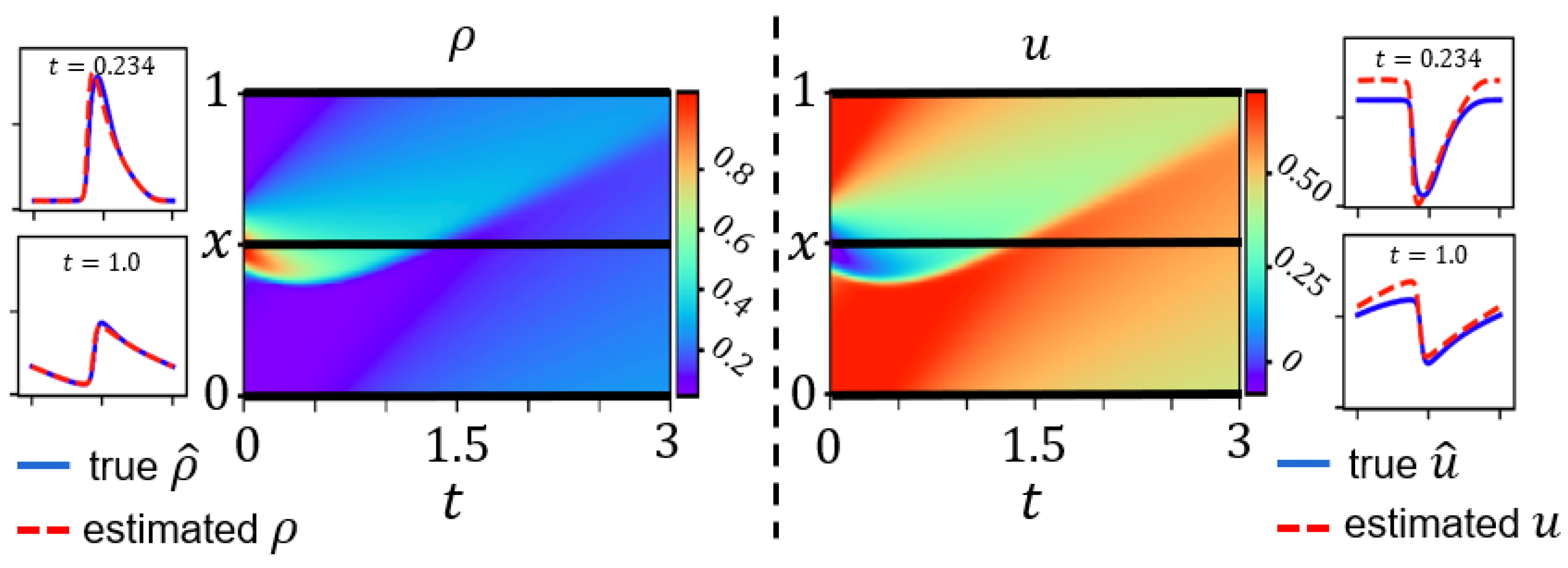
3.4. Numerical Data Validation for Three-Parameter-Based LWR

In this example, we show the ability of PIDL for the traffic dynamics governed by the three-parameter-based LWR traffic flow model on a ring road. Mathematically,
ρ t + ( Q ( ρ ) ) x = ϵ ρ x x , x [ 0 , 1 ] , t [ 0 , 3 ] ,
where ϵ = 0.005 . The initial and boundary conditions are ρ ( x , 0 ) = 0.1 + 0.8 e 25 ( x 0.5 ) 2 and ρ ( 0 , t ) = ρ ( 1 , t ) .
In this model, a three-parameter flux function [21] is employed: Q ( ρ ) = ρ U ( ρ ) = σ ( a + ( b a ) ρ ρ m a x 1 + y 2 ) , where a = 1 + ( δ p ) 2 , b = 1 + ( δ ( 1 p ) ) 2 and y = δ ( ρ ρ m a x p ) . In the model, δ , p, and σ are the three free parameters after which the function is named. The parameters σ and p control the maximum flow rate and critical density (where the flow is maximized), respectively. δ controls the roundness level of Q ( ρ ) . In addition to the above-mentioned three parameters, we also have ρ m a x and the diffusion coefficient ϵ as part of the model parameters. In this numerical example, we set δ = 5 , p = 2 , σ = 1 , ρ m a x = 1 , and ϵ = 0.005 .
Given the bell-shaped initial density condition, we apply the Godunov scheme to solve Equation (9) on 240 (space) × 960 (time) grid points evenly deployed throughout the [ 0 , 1 ] × [ 0 , 3 ] domain.
The PIDL architecture that encodes the LWR model is shown in Figure 6. This architecture consists of a PUNN for traffic density estimation, followed by a PICG for calculating the residual r c : = ρ t + ( Q ( ρ ) ) x ϵ ρ x x on collocation points. The estimated traffic density ρ is calculated by the PUNN f θ ( x , t ) , which is an NN and maps a spatiotemporal point ( x , t ) directly to ρ , i.e., ρ = f θ ( x , t ) . PUNN f θ ( x , t ) , parameterized by θ , is designed as a fully connected feedforward neural network with 8 hidden layers and 20 hidden nodes in each hidden layer. The hyperbolic tangent function (tanh) is used as the activation function for hidden neurons. By replacing ρ with f θ , we have r c : = [ f θ ] t + ( Q ( f θ ) ) x ϵ [ f θ ] x x in this case. With the estimated ρ and the observations ρ ^ on the observation points, we can obtain the data loss L o . In contrast, in PICGs, the connecting weights are fixed and the activation function of each node is designed to conduct a specific nonlinear operation for calculating an intermediate value of  r c . The physics discrepancy L c is the mean square of r c on the collocation points.
To customize the training of PIDL to Equation (9), we need to additionally introduce boundary collocation points  C B = { ( 0 , t ( i b ) ) | i b = 1 , , N b } { ( 1 , t ( i b ) ) | i b = 1 , , N b } , for learning the two boundary conditions. Different from the B in Equation (8), observations on boundary points are not required here in C B . Then, we obtain the following loss:
L o s s θ = α · L o + β · L c + γ · L b ,
where , L o = α N o i = 1 N o | f θ ( x ( i ) , t ( i ) ) ρ ^ ( i ) | 2 ( d a t a l o s s ) , L c = β N c j = 1 N c | r c ( x ( j ) , t ( j ) ) | 2 ( p h y s i c s l o s s ) , L b = γ N b i b = 1 N b | f θ ( 0 , t ( i b ) ) f θ ( 1 , t ( i b ) ) | 2 ( b o u n d a r y l o s s ) .
Note that because r c : = [ f θ ] t + ( Q ( f θ ) ) x ϵ [ f θ ] x x , r c is affected by θ . Furthermore, boundary collocation points are used to calculate the boundary loss L b . Because L b might change with different scenarios, it is ignored in Figure 6 for simplicity.
TSE and system identification using loop detectors: In this experiment, five model variables δ , p, σ , ρ m a x , and ϵ are encoded as learning variables in the PICG depicted in Figure 6. Define λ = ( δ , p , σ , ρ m a x , ϵ ) and the residual r c is affected by both θ and λ , resulting in the objective L o s s θ , λ . We now use observations from loop detectors, i.e., only the traffic density at certain locations where loop detectors are installed can be observed. By default, loop detectors are evenly located along the road.
We use N c = 150 , 000 collocation points and other experimental configurations are given in Appendix A.1.1. We conduct PIDL-based TSE experiments using different numbers of loop detectors to solve ( θ , λ ) = argmin θ , λ L o s s θ , λ . In addition to the traffic density estimation errors of ρ ( x , t ; θ ) , we evaluate the estimated model parameters λ using the L 2 relative error (RE) and present them as a percentage. Figure 7 presents a visualization of the estimated traffic density ρ (left) and traffic velocity (right) of the PIDL. Comparisons at certain time points are presented. Note that the PUNN in Figure 6 does not predict u directly, instead it is calculated by Q ( ρ ) / ρ in the post-processing.
More results are provided in Table A1 and the observation is that the PIDL architecture in Figure 6 with five loop detectors can achieve a satisfactory performance on both traffic density estimation and system identification. In general, more loop detectors can help our model to improve the TSE accuracy, as well as the convergence to the true model parameters. Specifically, for five loop detectors, an estimation error of 3.186 × 10 2 is obtained, and the model parameters converge to δ = 4.86236 , p = 0.19193 , σ = 0.10697 , ρ m a x = 1.00295 , and ϵ = 0.00515 , which are decently close to the ground-truth. The observations demonstrate that PIDL can handle both TSE and system identification with five loop detectors for the traffic dynamics governed by the three-parameter-based LWR.
We conduct sensitivity analysis on different numbers of collocation points and how they are identified. The details are presented in Table A2: A larger collocation rate (i.e., the ratio of the number of collocation points to the number of grid points) is beneficial for both TSE and system identification, because it could make the estimation on the collocation points physically consistent by imposing more constraints on the learning process. Empirically, more collocation points can cause a longer training time and the performance does not improve too much when a certain collocation rate is reached.

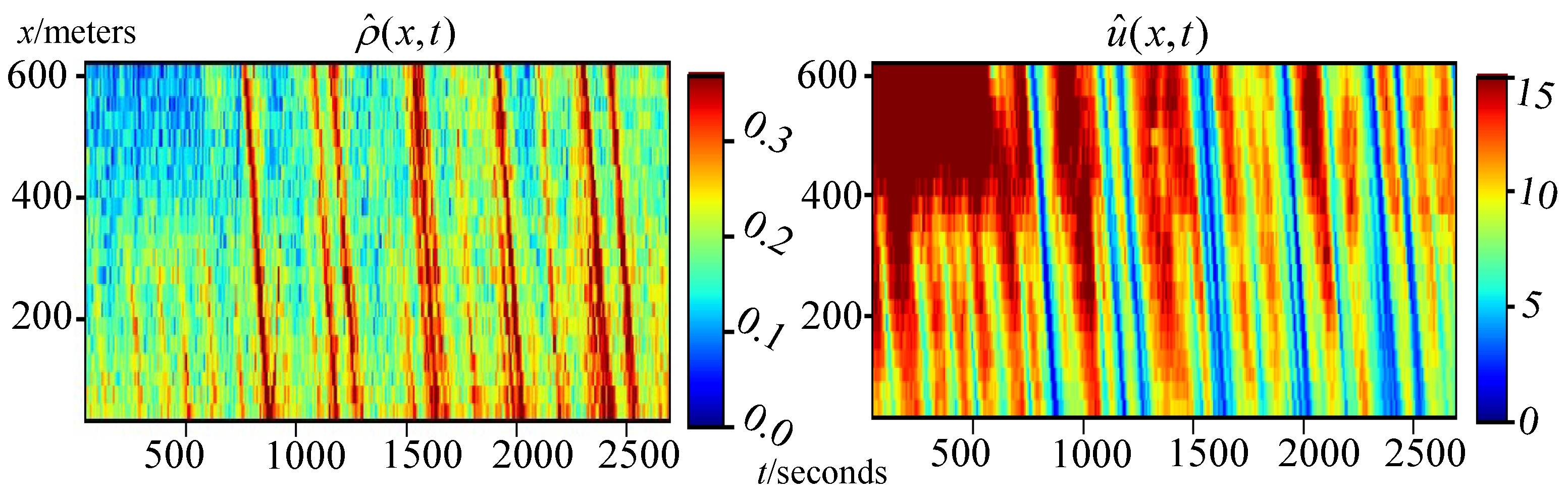
3.5. Real-World Data Validation

It would be interesting to see the performance of state-of-the-art methods based on either physics or data-driven approaches in order to better quantify the added value of the proposed class of approaches. We will use a widely used real-world open dataset, the next generation simulation (NGSIM) dataset, detailed in Table 3. Figure 8 plots the traffic density heatmap using data collected from the US 101 highway.
The performances of two baseline models and four PIDL variants for deterministic TSE are presented in Figure 9. As shown on the y-axis, the REs of the traffic density and velocity are used for evaluation. The comparison is made under representative combinations of the probe vehicle ratios (see x-axis) and numbers of loop detectors (see the titles of the sub-figures). We implement an EKF and a pure NN model as the representative pure data-driven and physics-driven baseline approaches, respectively. The EKF makes use of the three parameter-based LWR as the core physics when conducting the estimation. The NN only contains the PUNN component in Figure 6, and uses the first term in Equation (10) as the training loss. Among the PIDL variants, the PIDL-LWR and PIDL-ARZ are the PIDL models that encode the three parameter-based LWR and Greenshields-based ARZ, respectively, into the PICG. PIDL-LWR-FDL and PIDL-ARZ-FDL are the variant models of PIDL-LWR and PIDL-ARZ, replacing the FD components in the PICG with an embedded neural network (i.e., the FD learner). Note, the FD leaner technique is the one introduced by [31].
Performance of baseline models: From the experimental results, it is observed that the performance of all of the models improves as the data amounts increase. The EKF method performs better than the NN method, especially when the number of observations is small. The results are reasonable because EKF is a physics-driven approach, making sufficient use of the traffic flow model to appropriately estimate unobserved values when limited data are available. However, the model cannot fully capture the complicated traffic dynamics in the real world and the performance improves slowly as the data amount increases. The NN is able to catch up with the EKF when the amount of data is relatively large (see the case with loop = 2 and ratio = 3.0%). However, its data efficiency is low and large amounts of data are needed for accurate TSE.
Comparison between PIDL-based models: The PIDL-based approaches generally outperform the baseline models. PIDL-ARZ achieves lower errors than PIDL-LWR, because the ARZ model is a second-order model which can capture more complicated traffic dynamics and inform the PIDL in a more sophisticated manner.
Effects of using FDL: Comparing the models with FD learner (PIDL-LWR-FDL and PIDL-ARZ-FDL) to the ones without (PIDL-LWR and PIDL-ARZ), the former generally show better data efficiency. In PIDL-LWR-FDL and PIDL-ARZ-FDL, the FD equation is replaced by an internal small neural network to learn the hidden FD relation of the real traffic dynamics. A proper integration of the internal neural network may avoid directly encoding the complicated terms in PIDL and trade off between the sophistication of the model-driven aspect of PIDL and the training flexibility, making the framework a better fit to the TSE problem.
Comparison between PIDL-FDL-based models: PIDL-LWR-FDL can achieve lower errors than PIDL-ARZ-FDL, implying that sophisticated traffic models may not always lead to a better performance, because the model may contain complicated terms that make the TSE performance sensitive to the PIDL structural design. With the NGSIM data, PIDL-LWR-FDL can balance the trade-off between the sophistication of PIDL and the training flexibility more properly.
Transition from pure physics-driven to data-driven TSE models: The contributions of the physics-driven and data-driven components can be controlled by tuning the hyperparameters α and β in Equation (10). Figure 10 shows how the optimal β / α ratio changes as the data size increases. The x-axis is the number of loop detectors, which represents the training data size. The y-axis is the optimal β / α corresponding to the minimally achievable estimation errors of the PIDL-LWR methods shown in Figure 9. The property of tuning hyperparameters enables the PIDL-based methods to make a smooth transition from a pure physics-driven to pure data-driven TSE model: in the sufficient data regime, by using a small β / α ratio, the PIDL performs more like a pure data-driven TSE model to make ample use of the traffic data and mitigate the issue that the real dynamics cannot be easily modeled by some simple PDEs, while in the “small” data regime, by using a large ratio, the PIDL behaves like a pure physics-driven model to generalize better to unobserved domains.

4. PIDL for UQ

It is a widely studied modeling and computational challenge to quantify how uncertainty propagates within dynamical systems that could result in cascading errors, unreliable predictions, and worst of all, non-optimal operation and management strategies. It is thus crucial to characterize uncertainties in traffic state estimators and, consequently, in traffic management that relies on TSE predictors. UQ for TSE using PIDL is still in its nascent stage.
Definition 4. 
Uncertainty quantification (UQ) aims to assess the robustness of the developed model and bound the prediction errors of dynamical systems by estimating the probability density of quantities with input features and boundary conditions [79]. Stochastic effects and uncertainties potentially arise from various sources, including variability and errors in measurements, dynamic actions of various entities, model biases, and discretization and algorithmic errors. In summary, there are two types of uncertainty in the context of TSE [79,80]:
  • Aleatoric uncertainty (or data uncertainty): an endogenous property of data and thus irreducible, coming from measurement noise, incomplete data, or a mismatch between training and test data.
  • Epistemic uncertainty (or knowledge uncertainty, systematic uncertainty, model discrepancy): a property of a model arising from inadequate knowledge of the traffic states. For example, traffic normally constitutes multi-class vehicles (e.g., passenger cars, motorcycles, and commercial vehicles). A single model can lead to insufficiency in capturing diversely manifested behaviors.
UQ is “as old as the disciplines of probability and statistics” [79]. In recent years, its explosive growth in large-scale applications has been bolstered by the advance of big data and new computational models and architectures. The conventional UQ techniques include but are not limited to: sensitivity analysis and robust optimization [81]; probabilistic ensemble methods and Monte- arlo methods with multi-level variants [82,83,84]; stochastic spectral methods [79]; and methods based on the Frobenius–Perron and Koopman operators [85,86] for dynamic systems.
Epistemic uncertainty arising from model discrepancies, often bias, can be compensated for by improved domain knowledge, which has received increasing attention, especially with the advance of PIDL. In the computational architecture of PIDL, the data component can be treated as a compensation term for inaccurate or biased physics supplied by the physics-based component. Thus, it is natural to generalize PIDL to UQ, where the physics-based component provides partial domain knowledge when stochasticity is propagated within highly nonlinear models, and the data-driven component learns extra randomness arising from both data and model errors.
Definition 5. 
UQ for traffic state estimation (UQ-TSE) aims to capture the randomness of traffic states s ^ = { ρ ^ , u ^ } by probabilistic models. It is assumed that s ^ follows the observational distribution, i.e., s ^ p d a t a ( s ^ | x , t ) . The goal of the UQ-TSE problem is to train a probabilistic model G θ parameterized by θ such that the distribution of the prediction s p θ ( s | x , t ) resembles the distribution of the observation s ^ p d a t a ( s ^ | x , t ) . One widely used metric to quantify the discrepancy between p d a t a and p θ is the reverse Kullback–Leibler (KL) divergence.
Since the majority of the literature on UQ-PIDL employs deep generative models, including generative adversarial networks (GANs) [87], normalizing flow [88], and variational autoencoder (VAE) [89], here we will focus on how to leverage deep generative models for UQ problems. Among them, physics-informed generative adversarial network (PhysGAN) is the most widely used model which has been applied to solve stochastic differential equations [90,91] and to quantify uncertainty in various domains [31,92]. Little work has been performed on using physics-informed VAE for the UQ-TSE problem, which can be a future direction.

4.1. PIDL-UQ for TSE

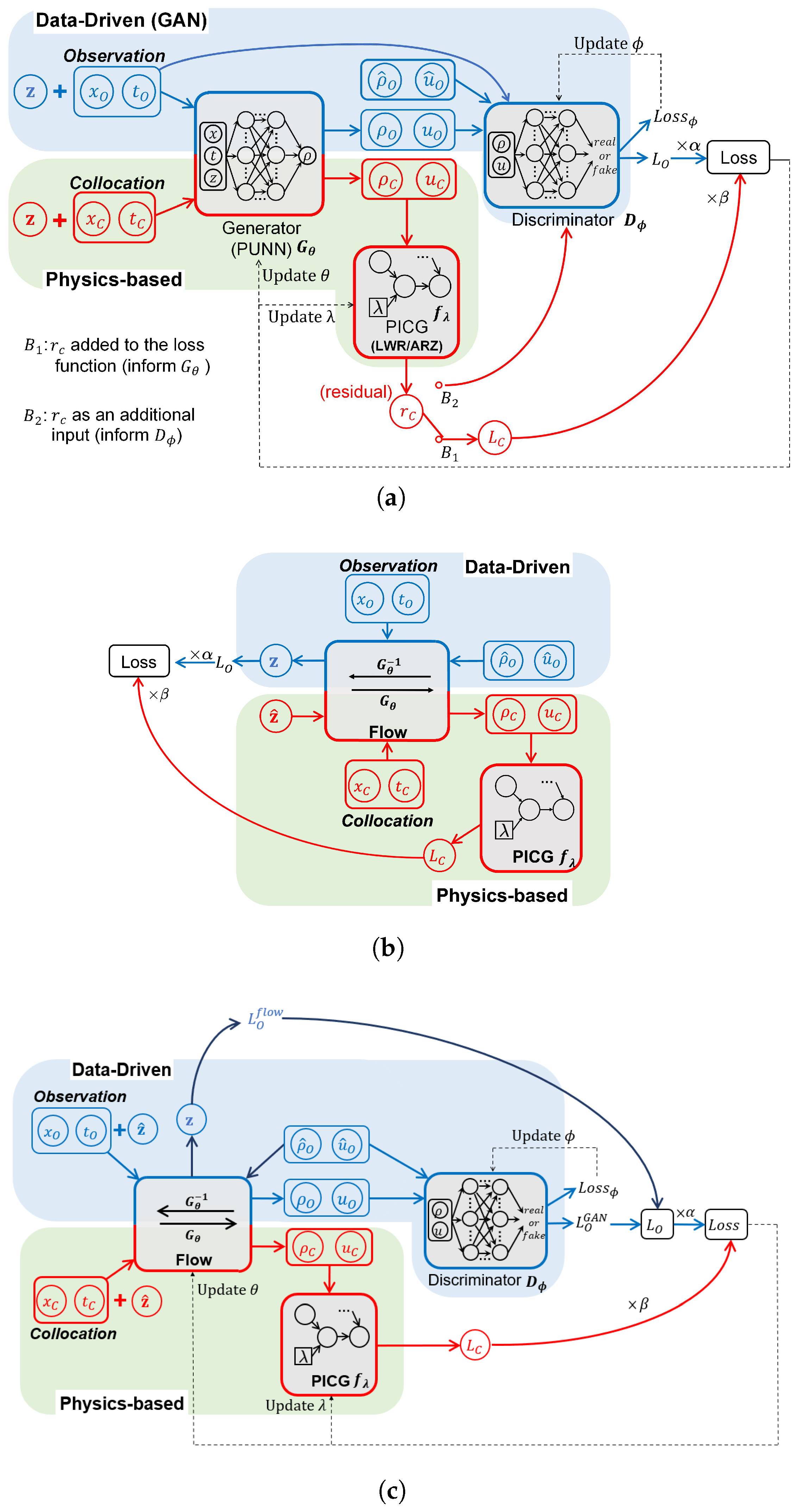
4.1.1. Physics-Informed Generative Adversarial Network (PhysGAN)

One way to formulate the UQ-TSE problem is to use a generative adversarial network (GAN) [87], which imitates the data distribution without specifying an explicit density distribution and can overcome the computational challenge of non-Gaussian likelihood [65], as opposed to using a Gaussian process [93,94].
Now, we will formulate the UQ problem in the context of conditional GANs. The generator G θ learns the mapping from the input ( x , t ) and a random noise z to the traffic state s , G θ : ( x , t , z ) s , where θ is the parameter of the generator. The objective of the generator G θ is to fool an adversarially trained discriminator D ϕ : ( x , t , s ) [ 0 , 1 ] . The loss functions of the GAN are depicted below:
L o s s θ ( g e n e r a t o r l o s s ) = E x , t , z D ϕ ( x , t , s ) 1 N o i = 1 N o D ϕ ( x ( i ) , t ( i ) , s ( i ) ) ,
L o s s ϕ ( d i s c r i m i n a t o r l o s s ) = E x , t , z ln D ϕ ( x , t , s ) E x , t , s ^ ln ( 1 D ϕ ( x , t , s ^ ) ) , 1 N o i = 1 N o ln D ϕ ( x ( i ) , t o ( i ) , s ( i ) ) + ln ( 1 D ϕ ( x ( i ) , t ( i ) , s ^ ( i ) ) ) ,
where s ( i ) = G θ ( x ( i ) , t ( i ) , z ( i ) ) is the predicted traffic state, and s ^ is the ground-truth. With physics imposed, the generator loss carries the same form as Equation (10), and the data loss L o and boundary loss L b become:
L o = 1 N o i = 1 N o D ϕ ( x ( i ) , t ( i ) , s ( i ) ) , L b = 1 N b i b = 1 N b D ϕ ( x ( i b ) , t ( i b ) , s ( i b ) ) .
Different PhysGAN variants adopt different ways of integrating physics into GANs, and the exact form of L c changes accordingly. Below we will introduce the general structure of the PhysGAN and its four variants.
The general structure of the PhysGAN is illustrated in Figure 11. The top blue box encloses the data-driven component, which is a GAN model consisting of a generator G θ and a discriminator D ϕ . Here, we omit details about how ρ and u interact within the generator. These two quantities can be generated sharing the same NN or from separate NNs. The PICG can be encoded with either the LWR or the ARZ equations.
PI-GAN Refs. [90,95,96] calculate the physics loss L c based on the residual r c , as illustrated in branch B 1 of Figure 11a. L c is added into the loss of the PUNN L o using the weighted sum. This model was the first and is the most widely used to encode physics into the generator.
PID-GAN Ref. [91] feeds the residual r c into the discriminator D ϕ to provide additional information on whether the predictions deviate from the physics equations, which helps the discriminator to distinguish between the prediction and the ground-truth. This way of integrating physics is illustrated in branch B 2 of Figure 11a. It is worth mentioning that the PID-GAN and the PI-GAN share the same structure of the data-driven component. They differ in how the physics are incorporated, i.e., informing the generator (branch B 1 ) or the discriminator (branch B 2 ). Ref. [91] shows that, by informing the discriminator, PID-GAN can mitigate the gradient imbalance issue of the PI-GAN.
The above-mentioned two PhysGAN variants use deterministic physics, that is, the parameters in the physics equations are deterministic.
Mean-GAN Ref. [97] incorporates stochastic differential equations into the physics components (illustrated as the PICG in Figure 11a), where physics parameters are assumed to follow Gaussian distributions. The randomness in the physics parameters is the source of the epistemic uncertainty, which leads to the randomness in the residual r c . The physics loss is calculated based on the square error in the mean of r c , i.e., | 1 N k i = 1 N k r c | 2 , where N k is the number of physics parameter samples. Then, the physics loss is included in the loss function of the PUNN using the weighted sum.
Within the PICG in Figure 11a, we can also replace the parametric FD with ML surrogates, which is used in the PI-GAN-FDL [65,98].

4.1.2. Physics-Informed Normalizing Flow (PhysFlow)

PhysFlow Ref. [99] employs the normalizing flow as an alternative generative model to the GAN. The normalizing flow explicitly estimates the likelihood, and is thus more straightforward to train compared to the GAN model. It estimates the likelihood by constructing an invertible function G θ that transforms a Gaussian prior z ^ to the traffic states s . The structure of the PhysFlow, i.e., PI-Flow, is illustrated in Figure 11b. The top blue box encloses the data-driven component, consisting of a normalizing flow model. The inverse function G θ 1 takes as input the traffic states and outputs a predicted prior z. The training objective is to make z follow a Gaussian distribution, which can be achieved by the maximum likelihood estimation. The bottom red box encloses the physics component, which is the same as the PI-GAN.

4.1.3. Physics-Informed Flow-Based GAN (PhysFlowGAN)

PhysFlowGAN combines the merits of GAN, normalizing flow, and PIDL. It uses normalizing flow as the generator for explicit likelihood estimation, while exploiting adversarial training with the discriminator to ensure sample quality. The structure of PhysFlowGAN is shown in Figure 11c, which consists of a normalizing flow, a discriminator, and a PICG. The data loss L o is composed of of two parts, i.e., L o G A N , that is calculated from the discriminator and L o f l o w , that is calculated from the normalizing flow. The physics loss is calculated in the same way as PI-GAN. One PhysFlowGAN model, TrafficFlowGAN [98], has been applied to the UQ-TSE problem.
Table 4 summarizes the hybrid architecture used for the UQ-TSE.

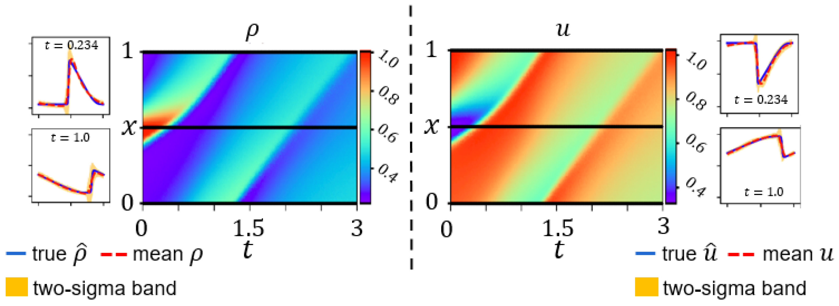
4.2. Numerical Data Validation for Greenshields-Based ARZ

As PI-GAN is the most widely used UQ-TSE model, we conduct numerical experiments using PI-GAN for demonstration. In the next subsection, we will use real-world data to compare the performance of the aforementioned UQ-TSE models.
The ARZ numerical data is generated from the Greenshields-based ARZ traffic flow model on a ring road:
ρ t + ( Q ( ρ ) ) x = 0 , x [ 0 , 1 ] , t [ 0 , 3 ] , t ( u + h ( ρ ) ) + u · x ( u + h ( ρ ) ) = ( U e q ( ρ ) u ) / τ , h ( ρ ) = U e q ( 0 ) U e q ( ρ ) .
U e q = u m a x ( 1 ρ / ρ m a x ) is the Greenshields speed function, where ρ m a x = 1.13 and u m a x = 1.02 , and τ is the relaxation time, which is set to 0.02. The boundary condition is ρ ( 0 , t ) = ρ ( 1 , t ) . The initial conditions of ρ and u are ρ ( x , 0 ) = 0.1 + 0.8 e 25 ( x 0.5 ) 2 and u ( x , 0 ) = 0.5 . Gaussian noise, following a distribution of N ( 0 , 0.02 ) , is added to impose randomness. The results of applying PI-GAN to ARZ numerical data are shown in Table A4. Figure 12 illustrates the predicted traffic density (left) and velocity (right) of the PI-GAN when the number of loop detectors is equal to three. The snapshots at sampled time steps show a good agreement between the prediction and the ground-truth.

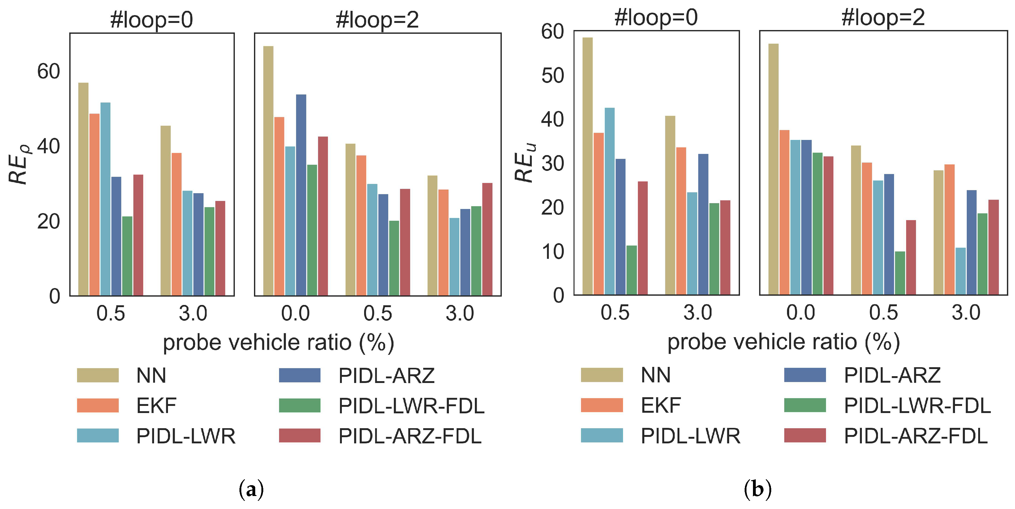
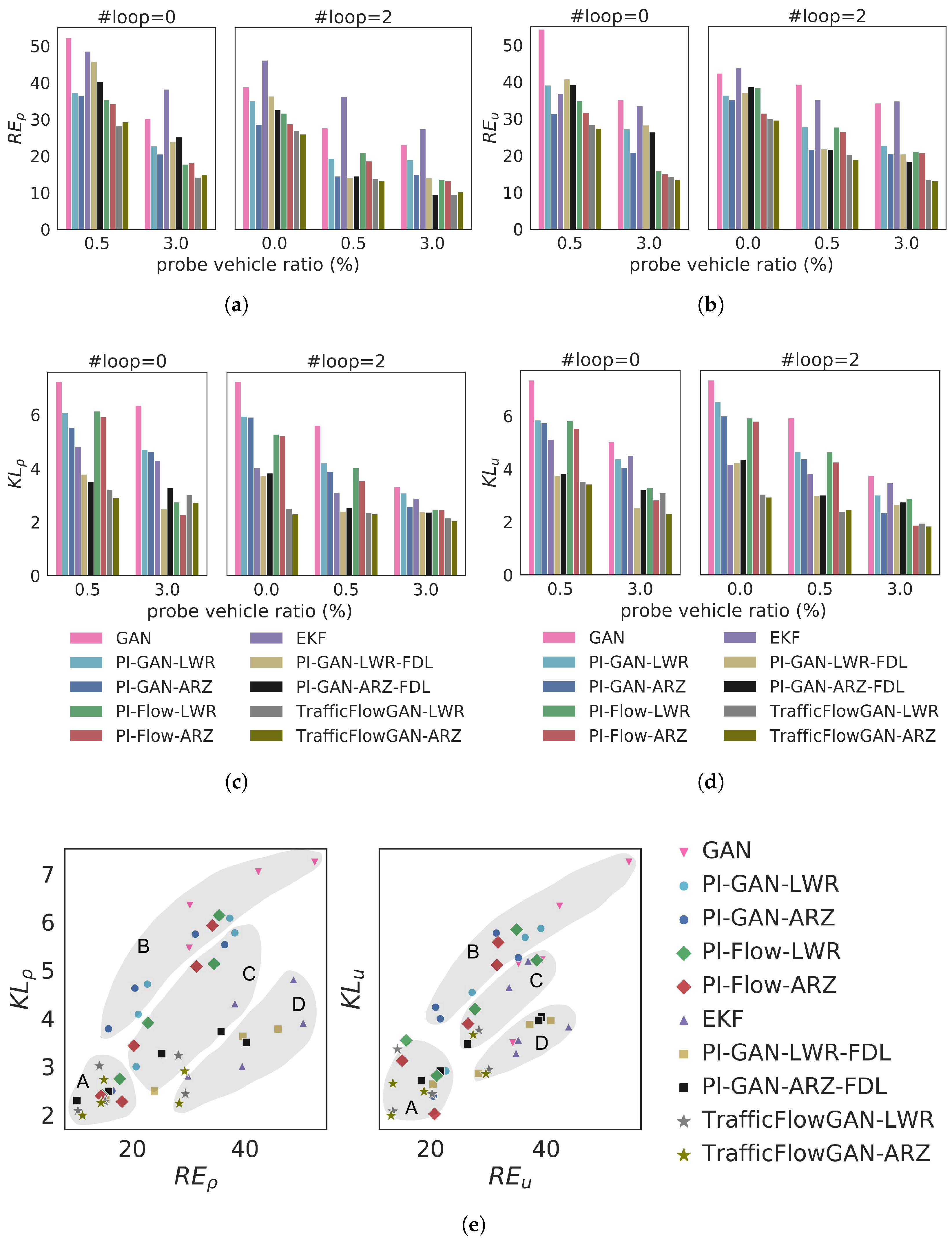
4.3. Real-World Data Validation

We apply PIDL-UQ models to the NGSIM dataset. We use four model types, i.e., PI-GAN, PI-GAN-FDL, PI-Flow, and TrafficFlowGAN for demonstration. Each model can be informed by either the LWR or ARZ equations, resulting in eight model variants in total. EKF and GAN are used as baselines. The EKF uses the three parameter-based LWR as the physics. The results are shown in Figure 13. As shown on the y-axis, the upper panels are the REs of the traffic density and velocity, and the lower panels are the Kullback–Leibler divergence (KL) of the traffic density and velocity. The comparison is made under representative combinations of probe vehicle ratios (see x-axis) and numbers of loop detectors (see the titles of sub-figures). We interpret the results from three perspectives:
Effect of loop data. When the probe vehicle ratio is fixed to 0.5%, the performance of all of the models is significantly improved as the loop number increases from 0 to 2, which is because the loop data provides more information. This improvement is not significant when the probe vehicle ratio is 3%, as the probe data alone has provided sufficient information.
Effects of using FDL. When the loop number is 2 and the probe vehicle ratio is 0.5%, PI-GAN-FDL achieves significantly lower REs and KLs compared to PI-GAN and PI-Flow, while this advantage becomes less significant when the data is sparse. This is because the ML surrogate requires more data to train. Furthermore, PI-GAN-FDL achieves lower KLs than PI-GAN in general, indicating that PI-GAN-FDL can better capture uncertainty.
Comparison between the ARZ-based model and the LWR-based model. The ARZ-based model outperforms the LWR-based model in general, which shows that the second-order physics is more suitable for the real-world scenario.
Comparison between PIDL-UQ models. As the data amount increases, the performance improves and the performance difference across models becomes small. Among all of the PIDL-based models, TrafficFlowGAN generally achieves the least error in terms of both RE and KL, because it combines the advantages of both PhysGAN and PhysFlow. In Figure 13e, we summarize the R E (x-axis), i.e., the relative difference between the predicted and ground-truth mean, and K L (y-axis), i.e., the statistical difference between the predicted and ground-truth distribution, of all of the models with different training datasets that are shown in Figure 13a–d. Each point represents a combination of metrics by applying one model type to one training dataset. We interpret these points by assigning them into four regions:
  • Region A (optimal RE and KL): Most points in this region belong to the TrafficFlowGAN model type (stars), which shows that the combination of PI-GAN and PI-Flow helps to achieve the best performance in terms of both RE and KL.
  • Region B (low RE and high KL): Most points in this region belong to GAN (inverted triangles) and PI-GAN (dots), which is a sign that the GAN-based models are prone to mode-collapse.
  • Region C (balanced RE and KL): Most points in this region belong to the PI-Flow model type, indicating that explicit estimation of the data likelihood helps to balance RE and KL.
  • Region D (high RE and low KL): Most points in this region belong to the EKF (triangles) and PI-GAN-FDL (squares), showing that these two types of model can better capture the uncertainty than the mean.
Transition from pure physics-driven to data-driven TSE models: Figure 14 shows the optimal β / α ratio of the TrafficFlowGAN under different numbers of loop detectors. The optimal β / α has a similar decreasing trend as in the deterministic TSE problem shown in Figure 10.

5. Conclusions and Future Work

5.1. Conclusions

This paper lays a methodological paradigm of PIDL for the TSE problem, including traffic state inference and uncertainty quantification. We present the concept of HCG that integrates both a PUNN and a PICG. In the TSE problem in particular, we present various architecture designs. For the traffic state inference problem, the PUNN and PICG can be linked in sequence or in parallel, depending on whether traffic velocity is computed from traffic density using FDs, or whether both velocity and density are computed from PUNN(s) simultaneously. For the UQ problem, GAN- and non-GAN-based adversarial generative models are presented to characterize the impact of measurement uncertainty on traffic states. The architecture variants, including PI-GAN, PID-GAN, Mean-GAN, PI-GAN-FDL, PI-Flow, and TrafficFlowGAN are introduced. This is the first study that compares PIDL model variants using the same real-world dataset, which provides a benchmark platform for model comparison. By comparing various PIDL models, we demonstrate that this paradigm is advantageous over pure physics- or data-driven approaches in the “small data” regime, and also allows a smooth transition from pure physics-driven to data-driven models via tuning the hyperparameters in the loss. Table 5 summarizes the existing types of hybrid architecture used in PIDL-TSE.

5.2. Outlook

Looking forward, we will pinpoint several promising research directions that we hope to guide researchers to exploit in this under-tapped area.

5.2.1. Physics Representation

What physics model is selected depends on the data fidelity, model fidelity, and available computational resources.
While there are a significant amount of models to describe traffic dynamics on micro- [100,101], meso- [102,103], and macro-scales [42,43,46,47], the future is in the discovery of a multiscale traffic model (i.e., a mapping from multiscale measurements to traffic states on different scales) that collectively infers traffic states with various measurements. Analytical multiscale models have been thoroughly studied in fields such as biological [13] and materials science [104], but remain under-exploited in transportation modeling. The drivers of developing a multiscale traffic model are two-fold: (1) Sensor data are at different scales. The collected traffic data include high-resolution individual trajectories and low-resolution aggregate information, both at various spatiotemporal granularity. Traffic measurements on different scales essentially measure the same system and phenomenon. Accordingly, a multiscale model, capable of integrating measurements of various scales, could characterize traffic dynamics more accurately with a smaller dataset [105]. (2) Traffic optimization and management strategies need to rely on diverse models and data of different scales. Individual traces are normally modeled using ODEs while aggregate traffic patterns are modeled with PDEs. An integrated ODE-PDE physics model can potentially accommodate these measurements at both the micro- and macro-scales [106]. Multiscale traffic models could also help to reduce model complexity and speed up simulation for real-time applications.
A multiscale traffic model, however, presents computational challenges due to the curse of dimensionality (i.e., high-dimensional input–output pairs). It is thus important to utilize reduced modeling techniques and multi-fidelity modeling [107,108,109].
An emerging direction to improve physics representation is to consider proxy models. For example, symbolic regression has been demonstrated to learn relatively simple physical forms to describe complex physical systems [110,111]. Traffic engineers have spent decades discovering various physical laws to describe human behavior models, such as car-following, lane-change, and other driving scenarios and tasks. Is it possible to develop a systematic method to select mathematical models? For example, the selection of a model can be reformulated as finding an optimal path over the PICG from inputs to outputs [112]. Accordingly, model selection is converted to an optimization problem. Machine learning methods, such as neural architecture search [113] and automatic modularization of network architecture [114], could enable the automatic architecture design of PICGs and PUNNs.

5.2.2. Learning Discontinuity in Patterns

Traffic patterns, especially congested traffic, are highly driven by underlying physics, thus, how to learn patterns around shockwaves, which correspond to discontinuities in which gradients do not exist, remains an active research area in PIDL. Ref. [115] introduces a convolutional neural network (CNN) for TSE, using a customized kernel, i.e., the anisotropic kernel, based on kinematic wave theory. Their anisotropic kernel specifies the influence region regarding the forward and backward traffic wave propagation characteristics. Fewer parameters are to be learned, making the training less computationally intensive. There is a small amount of literature that has discussed such a limitation using PIDL for nonlinear PDEs with solutions containing shocks and waves. One solution is to add viscosity terms [28,31,116] to smoothe the discontinuity.
Because the state of the art primarily focuses on the “soft” method, which imposes the physics constraints as part of the loss function, the fulfillment of physics constraints cannot be guaranteed, leading to poor prediction in shocks and waves. Thus, “hard” methods that enforce physics could be a radical remedy.

5.2.3. Transfer and Meta-Learning

For engineers, an important question is, if we have trained a PUNN using data collected from city A, can we directly generalize the prediction out of the NN using data from city B? Traffic datasets from two cities could differ drastically in the underlying traffic dynamics (arising from heterogeneity in driver behavior such as that in San Francisco and Mumbai), traffic environments, road conditions, initial and boundary conditions, and traffic demands. To address this challenge, we have to modify the input of the PUNN without using ( x , t ) but other attributes that vary across datasets, including, but not limited to, road type, geometry, lane width, lane number, speed limit, travel demands, traffic composition, and so on. One option is to employ Fourier neural operator (FNO) and its variants, e.g., the physics-informed FNO, to encode both the initial and boundary conditions as part of the inputs and to learn the nonlinear traffic-related operator directly, in other words, mapping ( x , t ) to the solutions associated with the given initial and boundary conditions [117]. Moreover, selection of training and validation datasets that can mitigate training bias would help with transfer learning, and one approach is to use an adversarial game [118] to select these two datasets and train a robust PIDL model.
Another direction to meet the transfer needs is to ask, how can we train a family of related physics-based PDEs (such as LWR and ARZ) and generalize the tuned hyperparameters to other physics members? Meta-learning the parameters involved in the PIDL pipeline could be a potential solution [119].

5.2.4. IoT Data for Urban Traffic Management

How can we fully exploit the advantage of multimodal, multi-fidelity IoT data, including, but not limited to, individual trajectories, camera images, radar heatmaps, and lidar cloud points? The existing practice is to preprocess these multimodal, multi-fidelity measurements using computer vision and extract aggregate traffic information in terms of traffic velocity and/or density within discretized spatial cells and time intervals. Rather than converting these data formats to conventional ones, we should think outside the box and potentially redefine the entire TSE framework. It thus demands a shift in paradigm from what constitutes traffic states to taking individual trajectories and images as inputs. In other words, is it sufficient to simply use aggregate traffic velocity, density, and flux to describe traffic states? The aggregate traffic measures were introduced decades ago when inductive loop detectors were deployed to measure cumulative traffic counts. Traffic flow has long been regarded as analogous to fluids, and, accordingly, hydrodynamic theory is applied to model traffic flow dynamics. It is natural to adapt physical quantities defined for fluids to traffic flow. However, traffic systems are not physical but social systems, in which road users constitute a complex traffic environment while interacting continuously with the built environment. Contextual information greatly influences driving behaviors and traffic dynamics. Accordingly, the question is, when we describe the state of traffic and aim to optimize traffic management strategies, would traffic contextual information perceived by our eyes and brains (represented by DNNs) be helpful as an addition to those widely used quantitative measures, especially when this type of information becomes more widely available thanks to IoT and smart city technology?
Furthermore, if TSE models can be enriched with multimodal data, what are the new challenges and opportunities to traffic control and optimization models that rely on traffic state inference? There are extensive studies on causal discovery and causal inference using observational data when unobserved counfounders are present [120,121]. However, little work has been performed to leverage explicit causal relations from physical knowledge to improve PIDL. For example, counterfactual analysis of physical dynamics concerns identifying the casual effects of various interventions, including traffic control and the sequential decision making of other agents in the environment [122,123,124]. Without performing extra experimentation that is risky and unsafe, how can we design and validate traffic management strategies using new information provided by IoT data?

5.2.5. TSE on Networks

With the ubiquitous sensors in smart cities, traffic state estimation on large-scale road networks will be more feasible and useful to perform. To generalize from single road segments to networks, the challenge lies in the spatial representation of graphs, as well as the temporal evolution of traffic dynamics. When PIDL is applied when there is sparse networked sensing information, we need to clarify in what representation existing physics models could be incorporated, in other words, how we should encode traffic states on links and those at junctions and into what deep learning models. Ref. [125] predicts network flows using a spatiotemporal differential equation network (STDEN) that integrates a differential equation network for the evolution of a traffic potential energy field into DNNs.
There are a lot more open questions that remain unanswered. As this field continues growing, we would like to leave them for readers to ponder:
  • How do we leverage various observation data to fully exploit the strengths of PIDL?
  • What types of sensors and sensing data would enrich the application domains of PIDL and better leverage its benefits?
  • Would there exist a universal architecture of hybrid computational graphs across domains?
  • What are robust evaluation methods and metrics for PIDL models against baselines?

Author Contributions

Conceptualization, X.D.; methodology, X.D., R.S., Z.M. and Y.F.; validation, R.S., Z.M. and Y.F.; formal analysis, R.S., Z.M. and Y.F.; writing—original draft preparation, X.D., R.S., Z.M. and Y.F.; writing—review and editing, X.D., R.S., Z.M. and Y.F.; supervision, X.D.; funding acquisition, X.D. All authors have read and agreed to the published version of the manuscript.

Funding

This work is sponsored by the National Science Foundation (NSF) under NSF CPS-2038984.

Data Availability Statement

Data is available at www.fhwa.dot.gov/publications/research/operations/07030/index.cfm; accessed on 22 May 2023.

Conflicts of Interest

The authors declare no conflict of interest.

Appendix A

Appendix A.1. Experimental Details for TSE and System Identification Using Loop Detectors

Appendix A.1.1. Experimental Configurations

The PUNN f θ ( x , t ) parameterized by θ is designed as a fully connected feedforward neural network with 8 hidden layers and 20 hidden nodes in each hidden layer. The specific structure is: layers = [2, 20, 20, 20, 20, 20, 20, 20, 20, 1], meaning that PUNN inputs ( x , t ) to estimate density ρ . The hyperbolic tangent function (tanh) is used as the activation function for each hidden neuron in PUNN. In addition, the PICG part in the PIDL architecture is parameterized by the physics parameters λ .
We train the PUNN and identify λ through the PIDL architecture using the adaptive moment estimation (Adam) optimizer [126] for a rough training for about 1000 iterations. A follow-up fine-grained training is performed by the limited-memory Broyden–Fletcher–Goldfarb–Shanno (L-BFGS) optimizer [127] for stabilizing the convergence, and the process terminates when the loss change of two consecutive steps is no larger than 10 16 . This training process converges to a local optimum ( θ , λ ) that minimizes the loss.
For a fixed number of loop detectors, we use grid search for hyperparameter tuning by default. Specifically, since the Adam optimizer is scale invariant, we fix the hyperparameter α to 100 and tune the other hyperparameters from [1, 10, 50, 100, 150, 200] with some follow-up fine tuning.
The training details are presented in Algorithm A1.
Algorithm A1: PIDL training for deterministic TSE.
1 Initialization:
2 Initialized PUNN parameters θ 0 ; Initialized physics parameters λ 0 ; Adam iterations I t e r ; Weights of loss functions α , β , and γ .
3 Input: The observation data O = { ( x ( i ) , t ( i ) , ρ ^ ( i ) ) } i = 1 N o ; collocation points
C = { ( x ( j ) , t ( j ) ) } j = 1 N c ; boundary collocation points C B , e.g.,
C B = { ( 0 , t ( i b ) ) } i b = 1 N b { ( 1 , t ( i b ) ) } i b = 1 N b
  1:
k 0
  2:
θ ˜ 0 ( θ 0 , λ 0 )
  3:
while  k < I t e r  do
  4:
    Calculate L o s s by Equation (10) using ( α , β , γ ) on ( O , C , C B )
  5:
     θ ˜ k + 1 θ ˜ k Adam ( θ ˜ k , θ ˜ L o s s )
 // use Adam for pre-training
  6:
     k k + 1
  7:
end while
  8:
while  θ ˜ k not converged do
  9:
    Calculate L o s s by Equation (10) using ( α , β , γ ) on ( O , C , C B )
  10:
     θ ˜ k + 1 θ ˜ k L-BFGS ( θ ˜ k , θ ˜ L o s s )
 // use L-BFGS for fine-grained training
  11:
     k k + 1
  12:
end while
  13:
return  θ ˜ k

Appendix A.1.2. Additional Experimental Results Using Numerical Data for Three-Parameter-Based LWR

The results under different numbers of loop detectors m are shown in Table A1.
Table A1. Prediction and parameter calibration errors of PIDL for the three-parameter-based LWR data.
m RE ρ (%) δ (%) p (%) σ (%) ρ max (%) ϵ (%)
375.5054.15124.52>1000>100099.95
410.0459.0772.63381.3114.606.72
53.1862.754.036.970.293.00
61.1250.692.492.260.497.56
80.76191.032.433.600.307.85
λ = ( δ , p , σ , ρ m a x , ϵ ) are estimated parameters, compared to the true parameters δ = 5 , p = 2 , σ = 1 , ρ m a x = 1 , ϵ = 0.005 .

Appendix A.1.3. Additional Experimental Results Using Real-World Data

Figure A1 shows the error heatmaps for the NN and PIDL-LWR-FDL models when the number of loop detectors is two and the prove vehicle ratio is 0.05, where “SE” means the squared error.
Figure A1. Error heatmaps of the NN and PIDL-LWR-FDL models. (a) S E ρ ( x , t ) of the PIDL-LWR-FDL; (b) S E ρ ( x , t ) of the NN.
Algorithms 16 00305 g0a1

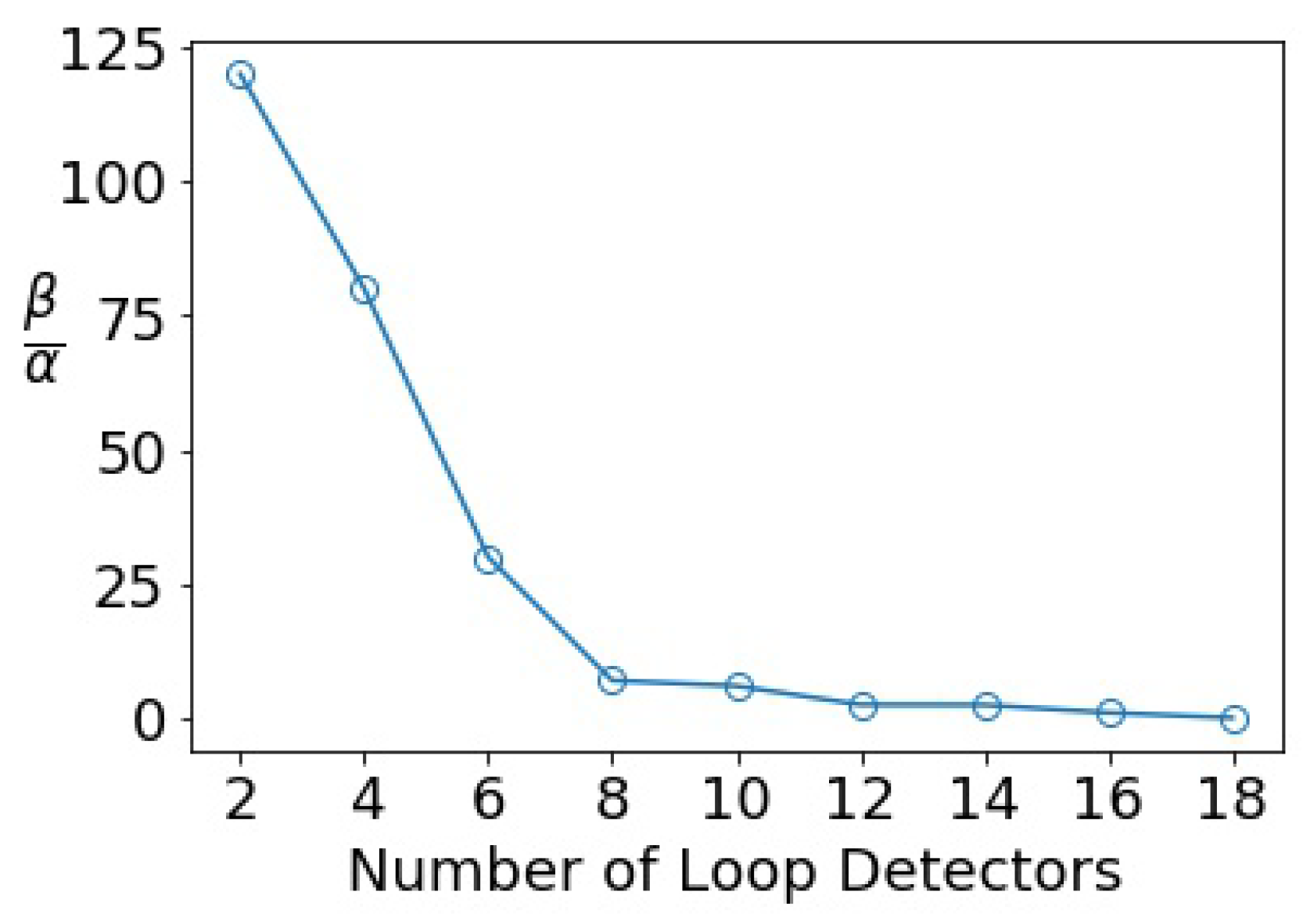
Appendix A.1.4. Sensitivity Analysis on Collocation Points

We conducted sensitivity analysis on different numbers of collocation points and the results are presented in Table A2. The detector number was fixed to five and the hyperparameters remained unchanged. The performances of estimation and parameter discovery improve when more collocation points are used. In this case study, the performance is sensitive to the number of collocations when the collocation rate is smaller than 0.01.
Table A2. Sensitivity analysis on collocation rates.
C . R . RE ρ (%) δ (%) p (%) σ (%) ρ max (%) ϵ (%)
0.000181.262.6621.15297.7725.91171.37
0.00110.264.5289.69504.2317.777.16
0.013.620.5511.1047.363.322.59
0.13.27.695.7415.780.453.41
0.53.01.884.235.870.603.37
C.R. stands for the collocation rate, which is the the ratio of the number of collocation points to the number of grid points. The detector number is fixed to 5.

Appendix A.1.5. Computational Effort and Model Accuracy

Table A3 presents the computational time and prediction error in the deterministic PIDL and baselines with the LWR model as the physics when the loop detector number is 2 and the probe vehicle ratio is 3 % . The first column is the name of the model used in the experiment, and the second column is the type of the model. The third and fourth columns are the computation times for the training and tests, respectively. The remaining columns are the performance metrics in terms of prediction error.
As EKF is not a learning-based method, it can make predictions directly after the parameters of the dynamic model, i.e., discrete LWR or ARZ, are pre-calibrated. Although the deep learning models (PIDL-FDL, NN) require training, their test time is much less than that of the EKF. In terms of accuracy, which is another aspect of evaluating the efficiency of a method, the PIDL and PIDL-FDL models achieve a significant accuracy improvement compared to EKF and NN. The short computational time in the test phase (or in the run time) and high accuracy are both of major consideration in real-world applications.
Table A3. The computation time and prediction error in deterministic PIDL models and baselines. (As EKF is not a learning-based method, the “training time” is not applicable to EKF).
ModelModel TypeComputation TimePrediction Error
Training
(s)
Test
(s)
RE ρ
( % )
RE u
( % )
EKFPhysics-based1.539.535.2
NNData-driven2480.0342.839.8
PIDLHybrid6470.0431.530.5
PIDL-FDLHybrid7690.0421.211.6

Appendix A.2. Experimental Details for UQ-TSE and System Identification Using Loop Detectors

Appendix A.2.1. Experimental Configurations

For the PI-GAN model, the generator structure is: layers = [3, 20, 40, 60, 80, 60, 40, 20, 2], meaning that the generator inputs ( x , t , z ) to estimate both the traffic density ρ and traffic velocity u. The discriminator structure is: layers = [4, 20, 20, 40, 60, 80, 60, 40, 20, 20, 1], meaning that the discriminator inputs ( x , t , ρ , u ) and outputs a one-dimensional real number indicating whether the input ρ and u are from the real-world data or not. Note that the discriminator has a more complex structure than the generator to stabilize the training. The rectified linear unit (ReLU) is used as the activation function for each hidden layer.
For the PI-Flow model, both the scale neural network and the transition neural network share the same structure, i.e., 2 hidden layers with 64 neurons in each layer. The number of transformations is six, that is, there are six scale neural networks and six transition neural networks in total. Leaky Relu is used as the activation function for each hidden layer.
For the TrafficFlowGAN, its PUNN is a normalizing flow model that shares the same architecture as that in the PI-Flow model introduced above. The discriminator consists of a stack of three convolutional layers. The kernel size for each layer is three, and the number of channels of each layer is 4, 8, and 16.
We use the Adam optimizer to train the neural networks for 5000 iterations. Different from training PIDL for deterministic TSE, the L-BFGS optimizer is not used, because the GAN model requires training the generator and discriminator in turn, for which the L-BFGS optimizer is not suitable. We fix the hyperparameter β = 1 α and tune α from [0.1, 0.3, 0.4, 0.6, 0.7].
The training details are presented in Algorithm A2.
Algorithm A2: PIDL-UQ training for stochastic TSE.
1 Initialization:
2 Initialized physics parameters λ 0 ; Initialized networks parameters θ 0 , ϕ 0 ; Training iterations I t e r ; Batch size m; Learning rate l r ; Weights of loss functions α , β , and γ .
3 Input: The observation data O = { ( x ( i ) , t ( i ) , ρ ^ ( i ) ) } i = 1 N o ; collocation points
C = { ( x ( j ) , t ( j ) ) } j = 1 N c ; boundary collocation points C B , e.g.,
C B = { ( 0 , t ( i b ) ) } i b = 1 N b { ( 1 , t ( i b ) ) } i b = 1 N b
  1:
for  k { 0 , . . . , I t e r } do
  2:
    Calculate L o s s by Equations (10) and (11) using ( α , β , γ ) on ( O , C , C B )
 // update the generator (PUNN)
  3:
     θ k + 1 ϕ k Adam ( θ k , θ L o s s )
  4:
    Calculate L o s s ϕ by Equation (12)
 // update the discriminator (for GAN, PhysGAN, and PhysFlowGAN)
  5:
     ϕ k + 1 ϕ k Adam ( ϕ k , ϕ L o s s ϕ )
  6:
end for

Appendix A.2.2. Additional Experimental Results Using Numerical Data Validation for Greenshields-Based ARZ

The results under different numbers of loop detectors m are shown in Table A4.
Table A4. Prediction and parameter calibration errors of PI-GAN for the Greenshields-based ARZ data.
m RE ρ (%) RE u (%) KL ρ KL u u max (%) ρ max (%)
342.632.51.3250.98511.515.6
430.220.90.9650.8356.54.5
620.611.80.7530.6382.92.2
818.56.30.6630.6212.31.9
m stands for the number of loop detectors. λ = ( ρ m a x , u m a x ) are estimated parameters, compared to the true parameters ρ m a x = 1.13 , u m a x = 1.02 .

Appendix A.2.3. Additional Experimental Results Using Real-World Data

Figure A2 shows the error and prediction standard deviation heatmaps for the EKF and TrafficFlowGAN models when the number of loop detectors is two and the prove vehicle ratio is 0.05.

Appendix A.2.4. Computational Time and Model Accuracy

Table A5 presents the computational time and prediction error of the stochastic PIDL-UQ with LWR model as the physics when the loop detector number is two and the probe vehicle ratio is 3 % . The column specification is the same as in Table A3, except for that there are more performance metrics for the UQ-TSE problem. The deep-learning-based models (GAN, PI-GAN, PI-Flow, and TrafficFlowGAN) achieve a much lower test time compared to the EKF, and there is a significant accuracy improvement for the PIDL-based models, especially for the TrafficFlowGAN model. This property is similar to what was seen Table A3 when training and testing the deterministic PIDL models. Among the PIDL-based models, PI-Flow has the shortest training time because it uses the normalizing flow model as the generator (PUNN), which can be trained by maximum likelihood estimation and does not require a discriminator. Using both normalizing flow and GAN, TrafficFlowGAN consumes the most time for training.
Figure A2. Error heatmaps of the EKF and TrafficFlowGAN. (a) S E ρ ( x , t ) of the TrafficFlowGAN; (b) S E ρ ( x , t ) of the EKF; (c) prediction’s standard deviation of the traffic density of the TrafficFlowGAN; (d) prediction’s standard deviation of the traffic density of the EKF.
Algorithms 16 00305 g0a2
Table A5. The computation time and prediction error of stochastic UQ-PIDL models and baselines. (As EKF is not a learning-based method, the “training time” is not applicable to EKF).
ModelModel TypeComputation TimePrediction Error
Training
(s)
Test
(s)
RE ρ
( % )
RE u
( % )
KL ρ
( % )
KL u
( % )
EKFPhysics-based1.539.535.23.003.32
GANData-driven32350.0330.139.35.455.12
PI-GANHybrid33260.0321.127.84.084.02
PI-GAN-FDLHybrid34530.0315.421.72.332.57
PI-FlowHybrid25480.0222.827.73.904.00
TrafficFlowGANHybrid43230.0215.220.32.272.07

Appendix A.3. Performance Metrics

We use four different metrics to quantify the performance of our models. In the formulas below, s ( x , t ) represents the predicted traffic state (i.e., traffic density ρ or traffic state u) at location x and time t, and s ^ represents the ground-truth.
  • Relative Error (RE) measures the relative difference between the predicted and ground-truth traffic states. For the deterministic TSE, RE is calculated by:
    RE s ( x , t ) = x t ( s ( x , t ) s ^ ( x , t ) ) 2 x t s ^ ( x , t ) 2 .
  • Squared Error (SE) measures the squared difference between the predicted and ground-truth traffic states at location x and time t. For the deterministic TSE, SE is calculated by:
    SE s ( x , t ) = ( s ( x , t ) s ^ ( x , t ) ) 2 .
  • Mean Squared Error (MSE) calculates the average SE over all locations and times, which is depicted as follows:
    M S E s ( x , t ) = x t S E s ( x , t ) / N
    where N is the total number of data.
  • Kullback–Leibler divergence (KL) measures the difference between two distributions P ( x ) and Q ( x ) , which is depicted as follows:
    KL ( P Q ) = x P ( x ) log P ( x ) Q ( x ) .
Note that for UQ-TSE, the traffic state s ( x , t ) follows a distribution, and the aforementioned errors measure the difference between the predicted and the ground-truth means instead. For example, RE and SE for the UQ-TSE are defined as:
RE s ( x , t ) = x t ( E [ s ( x , t ) ] E [ s ^ ( x , t ) ] ) 2 x t E [ s ^ ( x , t ) ] 2 .
SE s ( x , t ) = ( E [ s ( x , t ) ] E [ s ^ ( x , t ) ] ) 2 .

References

  1. Raissi, M.; Perdikaris, P.; Karniadakis, G.E. Physics-informed neural networks: A deep learning framework for solving forward and inverse problems involving nonlinear partial differential equations. J. Comput. Phys. 2019, 378, 686–707. [Google Scholar] [CrossRef]
  2. Karpatne, A.; Atluri, G.; Faghmous, J.H.; Steinbach, M.; Banerjee, A.; Ganguly, A.; Shekhar, S.; Samatova, N.; Kumar, V. Theory-guided data science: A new paradigm for scientific discovery from data. IEEE Trans. Knowl. Data Eng. 2017, 29, 2318–2331. [Google Scholar] [CrossRef]
  3. Yu, T.; Canales-Rodríguez, E.J.; Pizzolato, M.; Piredda, G.F.; Hilbert, T.; Fischi-Gomez, E.; Weigel, M.; Barakovic, M.; Cuadra, M.B.; Granziera, C.; et al. Model-informed machine learning for multi-component T2 relaxometry. Med. Image Anal. 2021, 69, 101940. [Google Scholar] [CrossRef] [PubMed]
  4. Karniadakis, G.E.; Kevrekidis, I.G.; Lu, L.; Perdikaris, P.; Wang, S.; Yang, L. Physics-informed machine learning. Nat. Rev. Phys. 2021, 3, 422–440. [Google Scholar] [CrossRef]
  5. Cuomo, S.; Di Cola, V.S.; Giampaolo, F.; Rozza, G.; Raissi, M.; Piccialli, F. Scientific Machine Learning through Physics-Informed Neural Networks: Where we are and What’s next. arXiv 2022, arXiv:2201.05624. [Google Scholar] [CrossRef]
  6. Di, X.; Shi, R. A survey on autonomous vehicle control in the era of mixed-autonomy: From physics-based to AI-guided driving policy learning. Transp. Res. Part Emerg. Technol. 2021, 125, 103008. [Google Scholar] [CrossRef]
  7. Huang, K.; Di, X.; Du, Q.; Chen, X. Stabilizing Traffic via Autonomous Vehicles: A Continuum Mean Field Game Approach. In Proceedings of the the 22nd IEEE International Conference on Intelligent Transportation Systems (ITSC), Auckland, New Zealand, 27–30 October 2019. [Google Scholar]
  8. Huang, K.; Di, X.; Du, Q.; Chen, X. Scalable traffic stability analysis in mixed-autonomy using continuum models. Transp. Res. Part Emerg. Technol. 2020, 111, 616–630. [Google Scholar] [CrossRef]
  9. Mo, Z.; Shi, R.; Di, X. A physics-informed deep learning paradigm for car-following models. Transp. Res. Part Emerg. Technol. 2021, 130, 103240. [Google Scholar] [CrossRef]
  10. Mo, Z.; Di, X. Uncertainty Quantification of Car-following Behaviors: Physics-Informed Generative Adversarial Networks. In Proceedings of the 28th ACM SIGKDD in conjunction with the 11th International Workshop on Urban Computing (UrbComp2022), Washington, DC, USA, 15 August 2022. [Google Scholar]
  11. Wang, Y.; Papageorgiou, M. Real-time freeway traffic state estimation based on extended Kalman filter: A general approach. Transp. Res. Part Methodol. 2005, 39, 141–167. [Google Scholar] [CrossRef]
  12. Seo, T.; Bayen, A.M.; Kusakabe, T.; Asakura, Y. Traffic state estimation on highway: A comprehensive survey. Annu. Rev. Control 2017, 43, 128–151. [Google Scholar] [CrossRef] [Green Version]
  13. Alber, M.; Tepole, A.B.; Cannon, W.R.; De, S.; Dura-Bernal, S.; Garikipati, K.; Karniadakis, G.; Lytton, W.W.; Perdikaris, P.; Petzold, L.; et al. Integrating machine learning and multiscale modeling—Perspectives, challenges, and opportunities in the biological, biomedical, and behavioral sciences. NPJ Digit. Med. 2019, 2, 115. [Google Scholar] [CrossRef] [Green Version]
  14. Krishnapriyan, A.; Gholami, A.; Zhe, S.; Kirby, R.; Mahoney, M.W. Characterizing possible failure modes in physics-informed neural networks. Adv. Neural Inf. Process. Syst. 2021, 34, 26548–26560. [Google Scholar]
  15. Di, X.; Liu, H.; Davis, G. Hybrid Extended Kalman Filtering Approach for Traffic Density Estimation Along Signalized Arterials: Use of Global Positioning System Data. Transp. Res. Rec. 2010, 2188.1, 165–173. [Google Scholar] [CrossRef] [Green Version]
  16. Davis, G.A.; Kang, J.G. Estimating destination-specific traffic densities on urban freeways for advanced traffic management. Transp. Res. Rec. 1994, 1457, 143–148. [Google Scholar]
  17. Kang, J.G. Estimation of Destination-Specific Traffic Densities and Identification of Parameters on Urban Freeways Using Markov Models of Traffic Flow. Ph.D. Thesis, University of Minnesota, Minneapolis, MN, USA, 1995. [Google Scholar]
  18. Jabari, S.E.; Liu, H.X. A stochastic model of traffic flow: Theoretical foundations. Transp. Res. Part Methodol. 2012, 46, 156–174. [Google Scholar] [CrossRef]
  19. Seo, T.; Kusakabe, T.; Asakura, Y. Traffic state estimation with the advanced probe vehicles using data assimilation. In Proceedings of the 2015 IEEE 18th International Conference on Intelligent Transportation Systems, Gran Canaria, Spain, 15–18 September 2015; IEEE: Piscataway Township, NJ, USA, 2015; pp. 824–830. [Google Scholar]
  20. Cremer, M.; Papageorgiou, M. Parameter identification for a traffic flow model. Automatica 1981, 17, 837–843. [Google Scholar] [CrossRef]
  21. Fan, S.; Seibold, B. Data-fitted first-order traffic models and their second-order generalizations: Comparison by trajectory and sensor data. Transp. Res. Rec. 2013, 2391, 32–43. [Google Scholar] [CrossRef]
  22. Kurzhanskiy, A.A.; Varaiya, P. Active traffic management on road networks: A macroscopic approach. Philos. Trans. R. Soc. Math. Phys. Eng. Sci. 2010, 368, 4607–4626. [Google Scholar] [CrossRef]
  23. Fan, S.; Herty, M.; Seibold, B. Comparative model accuracy of a data-fitted generalized Aw-Rascle-Zhang model. arXiv 2013, arXiv:1310.8219. [Google Scholar] [CrossRef]
  24. Ngoduy, D. Kernel smoothing method applicable to the dynamic calibration of traffic flow models. Comput. Civ. Infrastruct. Eng. 2011, 26, 420–432. [Google Scholar] [CrossRef]
  25. Huang, J.; Agarwal, S. Physics informed deep learning for traffic state estimation. In Proceedings of the IEEE 23rd International Conference on Intelligent Transportation Systems (ITSC), Rhodes, Greece, 20–23 September 2020; pp. 3487–3492. [Google Scholar]
  26. Barreau, M.; Aguiar, M.; Liu, J.; Johansson, K.H. Physics-informed Learning for Identification and State Reconstruction of Traffic Density. In Proceedings of the 60th IEEE Conference on Decision and Control (CDC), Austin, TA, USA, 13–15 December 2021; pp. 2653–2658. [Google Scholar]
  27. Shi, R.; Mo, Z.; Huang, K.; Di, X.; Du, Q. Physics-informed deep learning for traffic state estimation. arXiv 2021, arXiv:2101.06580. [Google Scholar]
  28. Shi, R.; Mo, Z.; Di, X. Physics informed deep learning for traffic state estimation: A hybrid paradigm informed by second-order traffic models. In Proceedings of the AAAI Conference on Artificial Intelligence, virtually, 2–9 February 2021; Volume 35, pp. 540–547. [Google Scholar]
  29. Brunton, S.L.; Proctor, J.L.; Kutz, J.N. Discovering governing equations from data by sparse identification of nonlinear dynamical systems. Proc. Natl. Acad. Sci. USA 2016, 113, 3932–3937. [Google Scholar] [CrossRef] [Green Version]
  30. Liu, J.; Barreau, M.; Čičić, M.; Johansson, K.H. Learning-based traffic state reconstruction using probe vehicles. IFAC-PapersOnLine 2021, 54, 87–92. [Google Scholar] [CrossRef]
  31. Shi, R.; Mo, Z.; Huang, K.; Di, X.; Du, Q. A physics-informed deep learning paradigm for traffic state and fundamental diagram estimation. IEEE Trans. Intell. Transp. Syst. 2022, 23, 11688–11698. [Google Scholar] [CrossRef]
  32. Chen, X.; Lei, M.; Saunier, N.; Sun, L. Low-rank autoregressive tensor completion for spatiotemporal traffic data imputation. IEEE Trans. Intell. Transp. Syst. 2021, 23, 12301–12310. [Google Scholar] [CrossRef]
  33. Chen, X.; Yang, J.; Sun, L. A nonconvex low-rank tensor completion model for spatiotemporal traffic data imputation. Transp. Res. Part Emerg. Technol. 2020, 117, 102673. [Google Scholar] [CrossRef]
  34. SAS. The Connected Vehicle: Big Data, Big Opportunities. 2015. Available online: https://www.sas.com/content/dam/SAS/en_us/doc/whitepaper1/connected-vehicle-107832.pdf (accessed on 30 April 2022).
  35. Chopra, K.; Gupta, K.; Lambora, A. Future Internet: The Internet of Things-A Literature Review. In Proceedings of the 2019 International Conference on Machine Learning, Big Data, Cloud and Parallel Computing (COMITCon), Faridabad, India, 14–16 February 2019; pp. 135–139. [Google Scholar]
  36. Chettri, L.; Bera, R. A Comprehensive Survey on Internet of Things (IoT) Toward 5G Wireless Systems. IEEE Internet Things J. 2020, 7, 16–32. [Google Scholar] [CrossRef]
  37. Abboud, K.; Omar, H.A.; Zhuang, W. Interworking of DSRC and Cellular Network Technologies for V2X Communications: A Survey. IEEE Trans. Veh. Technol. 2016, 65, 9457–9470. [Google Scholar] [CrossRef]
  38. Meinrenken, C.J.; Shou, Z.; Di, X. Using GPS-data to determine optimum electric vehicle ranges: A Michigan case study. Transp. Res. Part Transp. Environ. 2020, 78, 102203. [Google Scholar] [CrossRef]
  39. Elbers, J.; Zou, J. A Flexible X-haul Network for 5G and Beyond. In Proceedings of the 2019 24th OptoElectronics and Communications Conference (OECC) and 2019 International Conference on Photonics in Switching and Computing (PSC), Fukuoka, Japan, 7–11 July 2019; pp. 1–3. [Google Scholar]
  40. Porambage, P.; Okwuibe, J.; Liyanage, M.; Ylianttila, M.; Taleb, T. Survey on Multi-Access Edge Computing for Internet of Things Realization. IEEE Commun. Surv. Tutor. 2018, 20, 2961–2991. [Google Scholar] [CrossRef] [Green Version]
  41. Greenshields, B.D.; Bibbins, J.R.; Channing, W.S.; Miller, H.H. A study of traffic capacity. In Highway Research Board Proceedings; National Research Council (USA), Highway Research Board: Washington, DC, USA, 1935; Volume 1935. [Google Scholar]
  42. Lighthill, M.J.; Whitham, G.B. On kinematic waves II. A theory of traffic flow on long crowded roads. Proc. R. Soc. Lond. Ser. Math. Phys. Sci. 1955, 229, 317–345. [Google Scholar]
  43. Richards, P.I. Shock waves on the highway. Oper. Res. 1956, 4, 42–51. [Google Scholar] [CrossRef]
  44. Payne, H.J. Model of freeway traffic and control. In Mathematical Model of Public System; Simulation Councils, Inc.: La Jilla, CA, USA, 1971; pp. 51–61. [Google Scholar]
  45. Whitham, G.B. Linear and Nonlinear Waves; John Wiley & Sons: New York, NY, USA, 1974; Volume 42. [Google Scholar]
  46. Aw, A.; Klar, A.; Rascle, M.; Materne, T. Derivation of continuum traffic flow models from microscopic follow-the-leader models. SIAM J. Appl. Math. 2002, 63, 259–278. [Google Scholar] [CrossRef]
  47. Zhang, H.M. A non-equilibrium traffic model devoid of gas-like behavior. Transp. Res. Part Methodol. 2002, 36, 275–290. [Google Scholar] [CrossRef]
  48. Turner, D.S. 75 Years of the Fundamental Diagram for Traffic Flow Theory. In Proceedings of the Greenshields Symposium, Woods Hole, MA, USA, 8–10 July 2008. [Google Scholar]
  49. Wang, Y.; Papageorgiou, M.; Messmer, A. Real-time freeway traffic state estimation based on extended Kalman filter: Adaptive capabilities and real data testing. Transp. Res. Part Policy Pract. 2008, 42, 1340–1358. [Google Scholar] [CrossRef]
  50. Wang, Y.; Papageorgiou, M.; Messmer, A.; Coppola, P.; Tzimitsi, A.; Nuzzolo, A. An adaptive freeway traffic state estimator. Automatica 2009, 45, 10–24. [Google Scholar] [CrossRef] [Green Version]
  51. Mihaylova, L.; Boel, R.; Hegiy, A. An unscented Kalman filter for freeway traffic estimation. In Proceedings of the 11th IFAC Symposium on Control in Transportation Systems, Delft, The Netherlands, 29–31 August 2006. [Google Scholar]
  52. Blandin, S.; Couque, A.; Bayen, A.; Work, D. On sequential data assimilation for scalar macroscopic traffic flow models. Phys. Nonlinear Phenom. 2012, 241, 1421–1440. [Google Scholar] [CrossRef]
  53. Mihaylova, L.; Boel, R. A particle filter for freeway traffic estimation. In Proceedings of the 43rd IEEE Conference on Decision and Control (CDC), Nassau, Bahamas, 14–17 December 2004; pp. 2106–2111. [Google Scholar]
  54. Hinton, G.E.; Osindero, S.; Teh, Y.W. A fast learning algorithm for deep belief nets. Neural Comput. 2006, 18, 1527–1554. [Google Scholar] [CrossRef] [PubMed]
  55. Zhong, M.; Lingras, P.; Sharma, S. Estimation of missing traffic counts using factor, genetic, neural, and regression techniques. Transp. Res. Part Emerg. Technol. 2004, 12, 139–166. [Google Scholar] [CrossRef]
  56. Ni, D.; Leonard, J.D. Markov chain Monte Carlo multiple imputation using Bayesian networks for incomplete intelligent transportation systems data. Transp. Res. Rec. 2005, 1935, 57–67. [Google Scholar] [CrossRef]
  57. Tak, S.; Woo, S.; Yeo, H. Data-driven imputation method for traffic data in sectional units of road links. IEEE Trans. Intell. Transp. Syst. 2016, 17, 1762–1771. [Google Scholar] [CrossRef]
  58. Li, L.; Li, Y.; Li, Z. Efficient missing data imputing for traffic flow by considering temporal and spatial dependence. Transp. Res. Part Emerg. Technol. 2013, 34, 108–120. [Google Scholar] [CrossRef]
  59. Tan, H.; Wu, Y.; Cheng, B.; Wang, W.; Ran, B. Robust missing traffic flow imputation considering nonnegativity and road capacity. Math. Probl. Eng. 2014. [Google Scholar] [CrossRef] [Green Version]
  60. Ma, X.; Tao, Z.; Wang, Y.; Yu, H.; Wang, Y. Long short-term memory neural network for traffic speed prediction using remote microwave sensor data. Transp. Res. Part Emerg. Technol. 2015, 54, 187–197. [Google Scholar] [CrossRef]
  61. Polson, N.G.; Sokolov, V.O. Deep learning for short-term traffic flow prediction. Transp. Res. Part Emerg. Technol. 2017, 79, 1–17. [Google Scholar] [CrossRef] [Green Version]
  62. Tang, J.; Zhang, X.; Yin, W.; Zou, Y.; Wang, Y. Missing data imputation for traffic flow based on combination of fuzzy neural network and rough set theory. J. Intell. Transp. Syst. 2020, 25, 439–454. [Google Scholar] [CrossRef]
  63. Raissi, M. Deep hidden physics models: Deep learning of nonlinear partial differential equations. J. Mach. Learn. Res. 2018, 19, 932–955. [Google Scholar]
  64. Raissi, M.; Karniadakis, G.E. Hidden physics models: Machine learning of nonlinear partial differential equations. J. Comput. Phys. 2018, 357, 125–141. [Google Scholar] [CrossRef] [Green Version]
  65. Yang, Y.; Perdikaris, P. Adversarial uncertainty quantification in physics-informed neural networks. J. Comput. Phys. 2019, 394, 136–152. [Google Scholar] [CrossRef] [Green Version]
  66. Raissi, M.; Wang, Z.; Triantafyllou, M.S.; Karniadakis, G.E. Deep learning of vortex-induced vibrations. J. Fluid Mech. 2019, 861, 119–137. [Google Scholar] [CrossRef] [Green Version]
  67. Fang, Z.; Zhan, J. Physics-Informed Neural Network Framework For Partial Differential Equations on 3D Surfaces: Time Independent Problems. IEEE Access 2020. [Google Scholar]
  68. Raissi, M.; Yazdani, A.; Karniadakis, G.E. Hidden fluid mechanics: Learning velocity and pressure fields from flow visualizations. Science 2020, 367, 1026–1030. [Google Scholar] [CrossRef] [PubMed]
  69. Rai, R.; Sahu, C.K. Driven by data or derived through physics? a review of hybrid physics guided machine learning techniques with cyber-physical system (cps) focus. IEEE Access 2020, 8, 71050–71073. [Google Scholar] [CrossRef]
  70. Wang, K.; Sun, W.; Du, Q. A non-cooperative meta-modeling game for automated third-party calibrating, validating and falsifying constitutive laws with parallelized adversarial attacks. Comput. Methods Appl. Mech. Eng. 2021, 373, 113514. [Google Scholar] [CrossRef]
  71. Deng, W.; Lei, H.; Zhou, X. Traffic state estimation and uncertainty quantification based on heterogeneous data sources: A three detector approach. Transp. Res. Part Methodol. 2013, 57, 132–157. [Google Scholar] [CrossRef]
  72. Jagtap, A.D.; Kawaguchi, K.; Karniadakis, G.E. Adaptive activation functions accelerate convergence in deep and physics-informed neural networks. J. Comput. Phys. 2020, 404, 109136. [Google Scholar] [CrossRef] [Green Version]
  73. Li, Y.; Zhou, Z.; Ying, S. DeLISA: Deep learning based iteration scheme approximation for solving PDEs. J. Comput. Phys. 2022, 451, 110884. [Google Scholar] [CrossRef]
  74. Wang, S.; Yu, X.; Perdikaris, P. When and why PINNs fail to train: A neural tangent kernel perspective. J. Comput. Phys. 2022, 449, 110768. [Google Scholar] [CrossRef]
  75. Zhang, G.; Yu, Z.; Jin, D.; Li, Y. Physics-infused Machine Learning for Crowd Simulation. In Proceedings of the 28th ACM SIGKDD Conference on Knowledge Discovery and Data Mining, Washington, DC, USA, 14–18 August 2022; pp. 2439–2449. [Google Scholar]
  76. Boyd, S.; Parikh, N.; Chu, E.; Peleato, B.; Eckstein, J. Distributed optimization and statistical learning via the alternating direction method of multipliers. Found. Trends® Mach. Learn. 2011, 3, 1–122. [Google Scholar]
  77. Wang, J.; Yu, F.; Chen, X.; Zhao, L. ADMM for efficient deep learning with global convergence. In Proceedings of the 25th ACM SIGKDD International Conference on Knowledge Discovery and Data Mining (KDD), Anchorage, AK, USA, 4–8 August 2019; pp. 111–119. [Google Scholar]
  78. Barreau, M.; Liu, J.; Johanssoni, K.H. Learning-based State Reconstruction for a Scalar Hyperbolic PDE under noisy Lagrangian Sensing. In Proceedings of the 3rd Conference on Learning for Dynamics and Control (L4DC), Virtual Event, Switzerland, 7–8 June 2021; pp. 34–46. [Google Scholar]
  79. Smith, R.C. Uncertainty Quantification: Theory, Implementation, and Applications; SIAM: Philadelphia, PA, USA, 2013; Volume 12. [Google Scholar]
  80. Abdar, M.; Pourpanah, F.; Hussain, S.; Rezazadegan, D.; Liu, L.; Ghavamzadeh, M.; Fieguth, P.; Cao, X.; Khosravi, A.; Acharya, U.R.; et al. A review of uncertainty quantification in deep learning: Techniques, applications and challenges. Inf. Fusion 2021, 76, 243–297. [Google Scholar] [CrossRef]
  81. Bertsimas, D.; Brown, D.B.; Caramanis, C. Theory and applications of robust optimization. SIAM Rev. 2011, 53, 464–501. [Google Scholar] [CrossRef]
  82. Giles, M.B. Multilevel monte carlo path simulation. Oper. Res. 2008, 56, 607–617. [Google Scholar] [CrossRef] [Green Version]
  83. Sun, Q.; Du, Q.; Ming, J. Asymptotically Compatible Schemes for Stochastic Homogenization. SIAM J. Numer. Anal. 2018, 56, 1942–1960. [Google Scholar] [CrossRef]
  84. Efendiev, Y.; Hou, T.; Luo, W. Preconditioning Markov chain Monte Carlo simulations using coarse-scale models. SIAM J. Sci. Comput. 2006, 28, 776–803. [Google Scholar] [CrossRef] [Green Version]
  85. Brunton, S.L.; Brunton, B.W.; Proctor, J.L.; Kutz, J.N. Koopman invariant subspaces and finite linear representations of nonlinear dynamical systems for control. PLoS ONE 2016, 11, e0150171. [Google Scholar] [CrossRef] [PubMed] [Green Version]
  86. Dietrich, F.; Thiem, T.N.; Kevrekidis, I.G. On the Koopman Operator of Algorithms. SIAM J. Appl. Dyn. Syst. 2020, 19, 860–885. [Google Scholar] [CrossRef] [Green Version]
  87. Goodfellow, I. Nips 2016 tutorial: Generative adversarial networks. arXiv 2016, arXiv:1701.00160. [Google Scholar]
  88. Dinh, L.; Sohl-Dickstein, J.; Bengio, S. Density estimation using real nvp. arXiv 2016, arXiv:1605.08803. [Google Scholar]
  89. Kingma, D.P.; Welling, M. Auto-encoding variational bayes. arXiv 2013, arXiv:1312.6114. [Google Scholar]
  90. Yang, L.; Zhang, D.; Karniadakis, G.E. Physics-informed generative adversarial networks for stochastic differential equations. SIAM J. Sci. Comput. 2020, 42, A292–A317. [Google Scholar] [CrossRef] [Green Version]
  91. Daw, A.; Maruf, M.; Karpatne, A. PID-GAN: A GAN Framework based on a Physics-informed Discriminator for Uncertainty Quantification with Physics. In Proceedings of the 27th ACM SIGKDD Conference on Knowledge Discovery & Data Mining, Singapore, 14–18 August 2021; pp. 237–247. [Google Scholar]
  92. Siddani, B.; Balachandar, S.; Moore, W.C.; Yang, Y.; Fang, R. Machine learning for physics-informed generation of dispersed multiphase flow using generative adversarial networks. Theor. Comput. Fluid Dyn. 2021, 35, 807–830. [Google Scholar] [CrossRef]
  93. Bilionis, I.; Zabaras, N. Multi-output local Gaussian process regression: Applications to uncertainty quantification. J. Comput. Phys. 2012, 231, 5718–5746. [Google Scholar] [CrossRef]
  94. Bajaj, C.; McLennan, L.; Andeen, T.; Roy, A. Robust learning of physics informed neural networks. arXiv 2021, arXiv:2110.13330. [Google Scholar]
  95. Zhang, D.; Lu, L.; Guo, L.; Karniadakis, G.E. Quantifying total uncertainty in physics-informed neural networks for solving forward and inverse stochastic problems. J. Comput. Phys. 2019, 397, 108850. [Google Scholar] [CrossRef] [Green Version]
  96. Yang, L.; Treichler, S.; Kurth, T.; Fischer, K.; Barajas-Solano, D.; Romero, J.; Churavy, V.; Tartakovsky, A.; Houston, M.; Prabhat, M.; et al. Highly-scalable, physics-informed GANs for learning solutions of stochastic PDEs. In Proceedings of the 2019 IEEE/ACM Third Workshop on Deep Learning on Supercomputers (DLS), Denver, CO, USA, 17 November 2019; IEEE: Piscataway Township, NJ, USA, 2019; pp. 1–11. [Google Scholar]
  97. Mo, Z.; Fu, Y.; Di, X. Quantifying Uncertainty In Traffic State Estimation Using Generative Adversarial Networks. In Proceedings of the 2022 IEEE 25th International Conference on Intelligent Transportation Systems (ITSC), Macau, China, 8–12 October 2022; IEEE: Piscataway Township, NJ, USA, 2022; pp. 2769–2774. [Google Scholar]
  98. Mo, Z.; Fu, Y.; Xu, D.; Di, X. TrafficFlowGAN: Physics-informed Flow based Generative Adversarial Network for Uncertainty Quantification. In Proceedings of the Joint European Conference on Machine Learning and Knowledge Discovery in Database; Springer: Berlin/Heidelberg, Germany, 2022. [Google Scholar]
  99. Guo, L.; Wu, H.; Zhou, T. Normalizing field flows: Solving forward and inverse stochastic differential equations using physics-informed flow models. J. Comput. Phys. 2022, 461, 111202. [Google Scholar] [CrossRef]
  100. Treiber, M.; Hennecke, A.; Helbing, D. Congested traffic states in empirical observations and microscopic simulations. Phys. Rev. 2000, 62, 1805. [Google Scholar] [CrossRef] [Green Version]
  101. Kesting, A.; Treiber, M.; Schönhof, M.; Helbing, D. Adaptive cruise control design for active congestion avoidance. Transp. Res. Part Emerg. Technol. 2008, 16, 668–683. [Google Scholar] [CrossRef]
  102. Zhou, X.; Taylor, J. DTALite: A queue-based mesoscopic traffic simulator for fast model evaluation and calibration. Cogent Eng. 2014, 1, 961345. [Google Scholar] [CrossRef]
  103. Di Gangi, M.; Cantarella, G.E.; Di Pace, R.; Memoli, S. Network traffic control based on a mesoscopic dynamic flow model. Transp. Res. Part Emerg. Technol. 2016, 66, 3–26. [Google Scholar] [CrossRef]
  104. Chinesta, F.; Cueto, E.; Abisset-Chavanne, E.; Duval, J.L.; El Khaldi, F. Virtual, digital and hybrid twins: A new paradigm in data-based engineering and engineered data. Arch. Comput. Methods Eng. 2018, 27, 105–134. [Google Scholar] [CrossRef] [Green Version]
  105. Lu, J. Connected and Automated Mobility Modeling on Layered Transportation Networks: Cross-Resolution Architecture of System Estimation and Optimization; Technical Report; Arizona State University: Tempe, AZ, USA, 2022. [Google Scholar]
  106. Delle Monache, M.L.; Liard, T.; Piccoli, B.; Stern, R.; Work, D. Traffic reconstruction using autonomous vehicles. SIAM J. Appl. Math. 2019, 79, 1748–1767. [Google Scholar] [CrossRef]
  107. Peherstorfer, B.; Willcox, K.; Gunzburger, M. Survey of multifidelity methods in uncertainty propagation, inference, and optimization. SIAM Rev. 2018, 60, 550–591. [Google Scholar] [CrossRef] [Green Version]
  108. Penwarden, M.; Zhe, S.; Narayan, A.; Kirby, R.M. Multifidelity modeling for physics-informed neural networks (pinns). J. Comput. Phys. 2022, 451, 110844. [Google Scholar] [CrossRef]
  109. Lu, J.; Li, C.; Wu, X.B.; Zhou, X.S. Traffic System State Identification with Integrated Traffic State, Model Parameter and Queue Profile Estimation: Nonlinear Programming Reformulation with Differentiable Traffic State Variables Across Resolutions. SSRN 2022. [Google Scholar] [CrossRef]
  110. Schmidt, M.; Lipson, H. Distilling free-form natural laws from experimental data. Science 2009, 324, 81–85. [Google Scholar] [CrossRef]
  111. Cranmer, M.; Sanchez Gonzalez, A.; Battaglia, P.; Xu, R.; Cranmer, K.; Spergel, D.; Ho, S. Discovering symbolic models from deep learning with inductive biases. Adv. Neural Inf. Process. Syst. 2020, 33, 17429–17442. [Google Scholar]
  112. Wang, K.; Sun, W.; Du, Q. A cooperative game for automated learning of elasto-plasticity knowledge graphs and models with AI-guided experimentation. Comput. Mech. 2019, 64, 467–499. [Google Scholar] [CrossRef] [Green Version]
  113. Elsken, T.; Metzen, J.H.; Hutter, F. Neural architecture search: A survey. J. Mach. Learn. Res. 2019, 20, 1997–2017. [Google Scholar]
  114. Chen, Y.; Friesen, A.L.; Behbahani, F.; Doucet, A.; Budden, D.; Hoffman, M.; de Freitas, N. Modular meta-learning with shrinkage. Adv. Neural Inf. Process. Syst. 2020, 33, 2858–2869. [Google Scholar]
  115. Thodi, B.T.; Khan, Z.S.; Jabari, S.E.; Menéndez, M. Incorporating kinematic wave theory into a deep learning method for high-resolution traffic speed estimation. IEEE Trans. Intell. Transp. Syst. 2022, 23, 17849–17862. [Google Scholar] [CrossRef]
  116. Fuks, O.; Tchelepi, H.A. Limitations of physics informed machine learning for nonlinear two-phase transport in porous media. J. Mach. Learn. Model. Comput. 2020, 1, 19–37. [Google Scholar] [CrossRef]
  117. Thodi, B.T.; Ambadipudi, S.V.R.; Jabari, S.E. Learning-based solutions to nonlinear hyperbolic PDEs: Empirical insights on generalization errors. arXiv 2023, arXiv:2302.08144. [Google Scholar]
  118. Mo, Z.; Di, X.; Shi, R. Robust Data Sampling in Machine Learning: A Game-Theoretic Framework for Training and Validation Data Selection. Games 2023, 14, 13. [Google Scholar] [CrossRef]
  119. Psaros, A.F.; Kawaguchi, K.; Karniadakis, G.E. Meta-learning PINN loss functions. J. Comput. Phys. 2022, 458, 111121. [Google Scholar] [CrossRef]
  120. Spirtes, P.; Glymour, C.N.; Scheines, R.; Heckerman, D. Causation, Prediction, and Search; MIT Press: Cambridge, MA, USA, 2000. [Google Scholar]
  121. Pearl, J. Causality; Cambridge University Press: Cambridge, UK, 2009. [Google Scholar]
  122. Meng, C.; Seo, S.; Cao, D.; Griesemer, S.; Liu, Y. When Physics Meets Machine Learning: A Survey of Physics-Informed Machine Learning. arXiv 2022, arXiv:2203.16797. [Google Scholar]
  123. Ruan, K.; Di, X. Learning Human Driving Behaviors with Sequential Causal Imitation Learning. In Proceedings of the 36th AAAI Conference on Artificial Intelligence, Virtually, 22 February–1 March 2022. [Google Scholar]
  124. Ruan, K.; Zhang, J.; Di, X.; Bareinboim, E. Causal Imitation Learning Via Inverse Reinforcement Learning. In Proceedings of the 11th International Conference on Learning Representations, Kigali, Rwanda, 1–5 May 2023. [Google Scholar]
  125. Ji, J.; Wang, J.; Jiang, Z.; Jiang, J.; Zhang, H. STDEN: Towards Physics-guided Neural Networks for Traffic Flow Prediction. Proc. AAAI Conf. Artif. Intell. 2022, 36, 4048–4056. [Google Scholar] [CrossRef]
  126. Kingma, D.P.; Ba, J. Adam: A method for stochastic optimization. In Proceedings of the 3rd International Conference on Learning Representations (ICLR), San Diego, CA, USA, 7–9 May 2015. [Google Scholar]
  127. Byrd, R.H.; Lu, P.; Nocedal, J.; Zhu, C. A limited memory algorithm for bound constrained optimization. SIAM J. Sci. Comput. 1995, 16, 1190–1208. [Google Scholar] [CrossRef]
Figure 1. Comparison of pure physics-based, data-driven, and hybrid paradigms (adapted from [2]).
Algorithms 16 00305 g001
Figure 2. Schematic of PDE solution approximation.
Algorithms 16 00305 g002
Figure 3. Data types for TSE (adapted from [12], including fixed location sensors (blue hexagons), roadside camera, and collocation points (black crosses)).
Algorithms 16 00305 g003
Figure 4. Fundamental diagram (red line) with data (blue dots).
Algorithms 16 00305 g004
Figure 5. Flowchart of joint training of PIDL.
Algorithms 16 00305 g005
Figure 6. PIDL flowchart for three-parameter-based LWR, consisting of a PUNN for traffic density estimation and a PICG for calculating the residual, where λ = ( δ , p , σ , ρ m a x , ϵ ) .
Algorithms 16 00305 g006
Figure 7. Estimated traffic density ρ (left) and traffic velocity u (right) of the PIDL when the number of loop detectors is 3, where the horizontal black lines in the heatmap represent the sensor positions. In each half, the prediction heatmap and snapshots at certain time points are presented. Note that the PUNN does not predict u directly, and instead, it is calculated by Q ( ρ ) / ρ in the post-processing.
Algorithms 16 00305 g007
Figure 8. Average traffic density and speed on US 101 highway. Heatmap for the traffic density (left) and velocity (right).
Algorithms 16 00305 g008
Figure 9. Results of the deterministic PIDL models for the NGSIM dataset. “#loop” stands for the number of loop detectors. (a) RE of the traffic density; (b) RE of the traffic velocity.
Algorithms 16 00305 g009
Figure 10. Ratios of the contributions made by the physics-based component and the data-driven component to the optimal performance of PIDL.
Algorithms 16 00305 g010
Figure 11. PIDL architecture for UQ-TSE. The PhysGAN (a) consists of a generator, a discriminator, and a PICG. The PhysFlow (b) consists of a normalizing flow and a PICG. The PhysFlowGAN (c) consists of a normalizing flow, a discriminator, and a PICG. In each subfigure, the top blue box encloses the data-driven component, and the bottom red box encloses the physics component. (a) PhysGAN architecture. In the data-driven component, the observation is used to calculate the discriminator loss function L o s s ϕ using Equation (12) and the data loss of the generator L O using Equation (13). In the physics-based component, the collocation points are used to calculate the residual r C using Equation (10), which is then used to calculate the physics loss of the generator L C with two different ways of incorporating the residuals. (b) PhysFlow architecture. In the data-driven component, the inverse flow function G θ 1 aims to map the observation to a prior that follows a Gaussian distribution. In the physics-based component, the flow function maps a Gaussian prior to the collocation points, and a PICG is used to calculate the physics loss L C as in PhysGAN. (c) PhysFlowGAN architecture. This combines the architectures of PhysGAN and PhysFlow.
Algorithms 16 00305 g011
Figure 12. Estimated traffic density ρ (left) and traffic velocity (right) of the PI-GAN when the number of loop detectors is equal to 3, where the horizontal black lines in the heatmap represent the positions of the loop detectors. In each half, the prediction heatmap and snapshots at certain time points are presented.
Algorithms 16 00305 g012
Figure 13. Results of the PIDL-UQ models for the NGSIM dataset. (a) RE of the traffic density; (b) RE of the traffic velocity; (c) KL of the traffic density; (d) KL of the traffic velocity; (e) summary of RE and KL of the traffic density and velocity of all data sizes.
Algorithms 16 00305 g013
Figure 14. Ratios of the contributions made by the physics-based component and the data-driven component to the optimal training of TrafficFlowGAN. β and α are hyperparameters in Equation (10) which control the contribution of the physics-based and data-driven components, respectively.
Algorithms 16 00305 g014
Table 1. State-of-the-art approaches for parameter calibration.
MethodDescription ρ max ρ critical u max
Max. DensityCritical DensityMax. Speed
Sequential trainingCalibrate each parameter separatelyEach parameter carries a certain physical meaningSegment length divided by avg. vehicle lengthTraffic density at capacitySpeed limit or max. value
Calibrate parameter and predict state jointlyAugment states with parameters estimated using DA [15,16,17,18]Tuning along with other hyperparameters in DNNs
Calibrate FDFit parameters associated with a pre-selected FD [19,20,21,22,23,24,25]Density at u = 0 Density at max q Velocity at maximum
Joint trainingCalibrate FDFit parameters associated with a pre-selected FD along with parameters of DNNs [26,27,28]Density at u = 0 Density at max q Velocity at maximum
ML surrogateReduce variable and parameter sizes while maintaining the minimum physical relevance [29,30,31]Parametrized in DNNsin
Table 2. State-of-the-art PIDL-TSE.
PhysicsDataDescriptionsRef.
First-order modelLWRSynthetic (Lax–Hopf method)Integrated the Greenshields-based LWR to PIDL and validated it using loop detectors as well as randomly placed sensors.[25]
LWRNumerical, NGSIMPresented the use of PIDL to solve Greenshields-based and three-parameter-based LWR models, and demonstrated its advantages using a real-world dataset.[27]
LWRNumericalStudied the general partial-state reconstruction problem for traffic flow estimation, and used PIDL encoded with LWR to counterbalance the small number of probe vehicle data.[78]
FL1, LWRSUMO simulationIntegrated a coupled micro–macro model, combining the follow-the-leader (FL1) model and LWR model, to PIDL for TSE, which can use the velocity information from probe vehicles.[26,30]
Second-order modelLWR and ARZNumerical, NGSIMApplied the PIDL-based TSE to the second-order ARZ with observations from both loop detectors and probe vehicles, and estimated both ρ and u in parallel.[28]
Proposed the idea of integrating ML surrogate (e.g., an NN) into the physics-based component in the PICG to represent the complicated FD relation. Improved estimation accuracy achieved and unknown FD relation learned.[31]
Table 3. Real-world data description.
SiteLocationDateLength (m)Sampling Rate (s)Lane #
US 101 1LA, CA6/15/20056400.15
Note: Vehicular information includes the position, velocity, acceleration, occupied lane, and vehicle class. Time periods include 7:50–8:05 a.m., 8:05–8:20 a.m., and 8:20–8:35 a.m. and the data is collected on 15 June 2005. The data remains accessible to date. We average traffic states across all lanes; 1 www.fhwa.dot.gov/publications/research/operations/07030/index.cfm; accessed on 22 May 2023.
Table 4. Architecture used for the UQ-TSE.
ModelDescriptionsProsRef.
PhysGANPI-GAN L c = 1 N c i = 1 N c | r c | 2 is added to the generator loss function using the weighted sum.The most widely used[65,90,95,96]
PID-GANResidual is fed into the discriminator, D ϕ ( x ( j ) , t ( j ) , s ( j ) , e | r c ( j ) | 2 ) , which is then averaged over collocation points to calculate L c .Can mitigate the gradient imbalance issue[91]
Mean-GANResidual is averaged over the physics parameter λ : L c = 1 N c i = 1 N c | 1 N k i = 1 N k r c | 2 .Can encode stochastic physics model[97]
PI-GAN-FDLThe ρ u relation is approximated by ML surrogates; physics loss L c is the same as PI-GAN.Requires minimal physics information[65,98]
PhysFlowPI-FlowThe normalizing flow model is used as the generator for explicit computation of the likelihood; the physics loss L c is the same as PI-GAN.Simple structure; easy to train[99]
PhysFlowGANTraffic Flow GANThe normalizing flow model is used as the generator for explicit computation of the likelihood; a convolutional neural network is used as the discriminator to ensure high sample quality physics loss L c is the same as PI-GAN.Combines the merits of PhysGAN and PhysFlow[98]
Table 5. Configuration of physics in the physics-based component.
PUNN-PICG TopologyPUNN HierarchySharedSeparate
Sequential[25,27,28,30,65,91,96,97,98][26,31,65,78,90,95,99]
Parallel[9,10]-
Note: PUNN-PICG topology refers to the layout between PUNN and PICG, which can be either “sequential” (i.e., the output of PUNN is the input into PICG, so PICG follows PUNN) or “parallel” (i.e., PUNN and PICG output predictions side-by-side to compute a loss). PUNN hierarchy refers to the layout of the NNs that are used to predict ρ and u. “Shared” means that only one NN is used to output both ρ and u, while “separate” means that two NNs are used to output ρ and u, respectively.
Disclaimer/Publisher’s Note: The statements, opinions and data contained in all publications are solely those of the individual author(s) and contributor(s) and not of MDPI and/or the editor(s). MDPI and/or the editor(s) disclaim responsibility for any injury to people or property resulting from any ideas, methods, instructions or products referred to in the content.

