
DrugFinder: Druggable Protein Identification Model Based on Pre-Trained Models and Evolutionary Information


Abstract
1. Introduction
2. Materials and Methods
2.1. Dataset
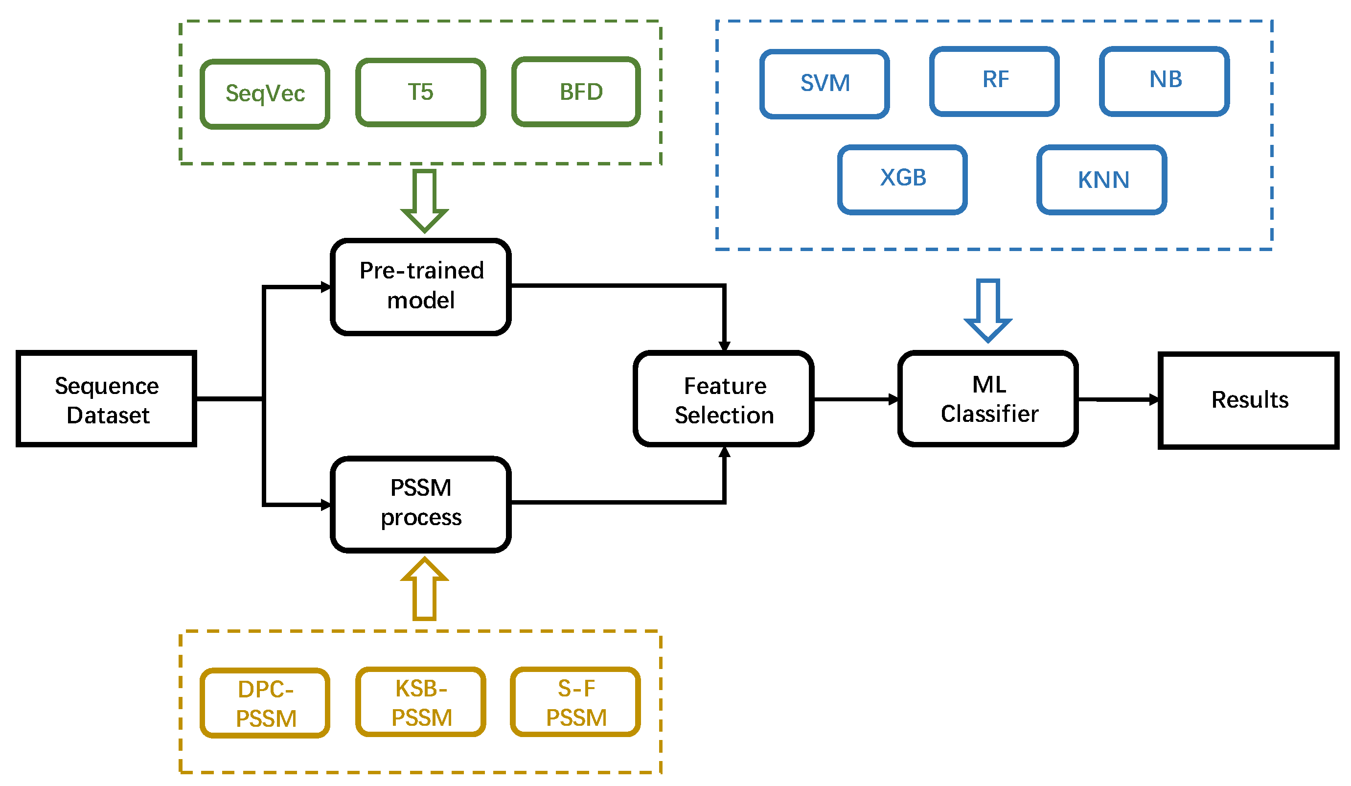
2.2. Methods
2.2.1. Pre-Trained Models
2.2.2. PSSM Process
2.2.3. Feature Selection
2.2.4. Machine Learning Classifier
2.2.5. Performance Evaluation
3. Results
3.1. Comparison of Pre-Trained Models
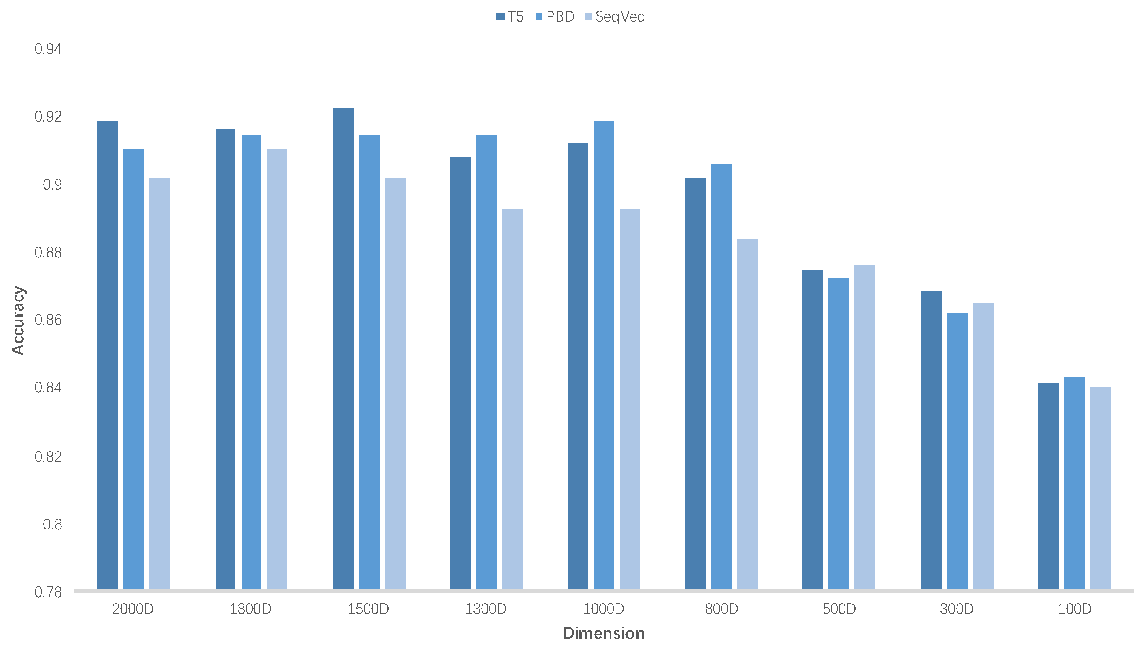
3.2. Feature Selection
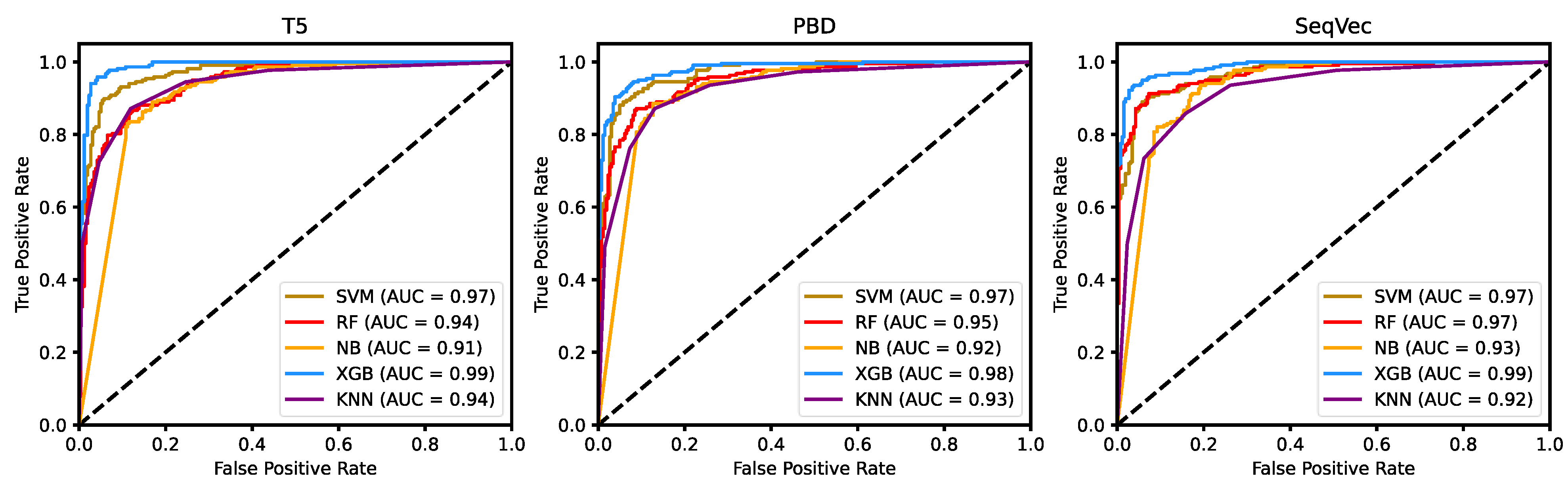
3.3. Machine Learning Classifier
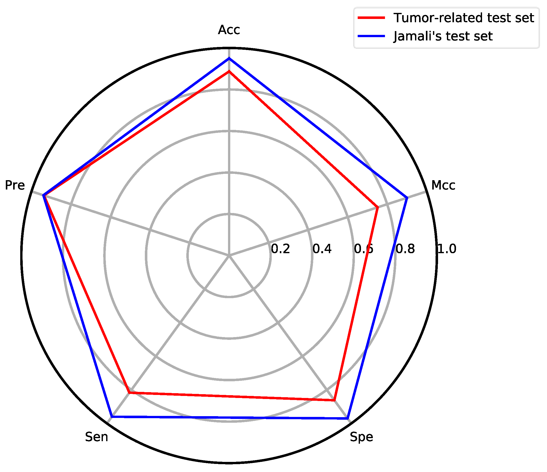
3.4. Model Performance on Specific Disease Target Test Set
3.5. Comparison with Other Models
4. Discussion
Author Contributions
Funding
Data Availability Statement
Conflicts of Interest
References
- Owens, J. Determining druggability. Nat. Rev. Drug Discov. 2007, 6, 187. [Google Scholar] [CrossRef]
- Wishart, D.S.; Feunang, Y.D.; Guo, A.C.; Lo, E.J.; Marcu, A.; Grant, J.R.; Sajed, T.; Johnson, D.; Li, C.; Sayeeda, Z.; et al. DrugBank 5.0: A major update to the DrugBank database for 2018. Nucleic Acids Res. 2018, 46, D1074–D1082. [Google Scholar] [CrossRef] [PubMed]
- Lacombe, D.; Butler-Smith, A.; Therasse, P.; Fumoleau, P.; Burtles, S.; Calvert, H.; Marsoni, S.; Sessa, C.; Verweij, J. Cancer drug development in Europe: A selection of new agents under development at the European Drug Development Network: NEW DRUGS. Cancer Investig. 2003, 21, 137–147. [Google Scholar] [CrossRef] [PubMed]
- Lombardino, J.G.; Lowe, J.A. The role of the medicinal chemist in drug discovery—Then and now. Nat. Rev. Drug Discov. 2004, 3, 853–862. [Google Scholar] [CrossRef] [PubMed]
- Roy, A. Challenges with risk mitigation in academic drug discovery: Finding the best solution. Expert Opin. Drug Discov. 2019, 14, 95–100. [Google Scholar] [CrossRef] [PubMed]
- Zhang, L.C.; Kong, L. iRSpot-ADPM: Identify recombination spots by incorporating the associated dinucleotide product model into Chou’s pseudo components. J. Theor. Biol. 2018, 441, 1–8. [Google Scholar] [CrossRef]
- Dai, Y.F.; Zhao, X.M. A Survey on the Computational Approaches to Identify Drug Targets in the Postgenomic Era. Biomed Res. Int. 2015, 2015, 239654. [Google Scholar] [CrossRef]
- Roh, Y.; Heo, G.; Whang, S.E. A Survey on Data Collection for Machine Learning: A Big Data-AI Integration Perspective. IEEE Trans. Knowl. Data Eng. 2021, 33, 1328–1347. [Google Scholar] [CrossRef]
- Yu, H.; Chen, J.X.; Xu, X.; Li, Y.; Zhao, H.H.; Fang, Y.P.; Li, X.X.; Zhou, W.; Wang, W.; Wang, Y.H. A Systematic Prediction of Multiple Drug-Target Interactions from Chemical, Genomic, and Pharmacological Data. PLoS ONE 2012, 7, e37608. [Google Scholar] [CrossRef]
- Huang, C.; Zhang, R.J.; Chen, Z.Q.; Jiang, Y.S.A.; Shang, Z.W.; Sun, P.; Zhang, X.H.; Li, X. Predict potential drug targets from the ion channel proteins based on SVM. J. Theor. Biol. 2010, 262, 750–756. [Google Scholar] [CrossRef]
- Jamali, A.A.; Ferdousi, R.; Razzaghi, S.; Li, J.Y.; Safdari, R.; Ebrahimie, E. DrugMiner: Comparative analysis of machine learning algorithms for prediction of potential druggable proteins. Drug Discov. Today 2016, 21, 718–724. [Google Scholar] [CrossRef] [PubMed]
- Lin, J.; Chen, H.; Li, S.; Liu, Y.; Li, X.; Yu, B. Accurate prediction of potential druggable proteins based on genetic algorithm and Bagging-SVM ensemble classifier. Artif. Intell. Med. 2019, 98, 35–47. [Google Scholar] [CrossRef] [PubMed]
- Yu, L.; Xue, L.; Liu, F.; Li, Y.; Jing, R.; Luo, J. The applications of deep learning algorithms on in silico druggable proteins identification. J. Adv. Res. 2022, 41, 219–231. [Google Scholar] [CrossRef]
- Sikander, R.; Ghulam, A.; Ali, F. XGB-DrugPred: Computational prediction of druggable proteins using eXtreme gradient boosting and optimized features set. Sci. Rep. 2022, 12, 1–9. [Google Scholar] [CrossRef] [PubMed]
- Chen, J.X.; Gu, Z.H.; Xu, Y.J.; Deng, M.H.; Lai, L.H.; Pei, J.F. QuoteTarget: A sequence-based transformer protein language model to identify potentially druggable protein targets. Protein Sci. 2023, 32, e4555. [Google Scholar] [CrossRef] [PubMed]
- Hochreiter, S.; Schmidhuber, J. Long Short-Term Memory. Neural Comput. 1997, 9, 1735–1780. [Google Scholar] [CrossRef] [PubMed]
- Wang, J.Y.; Hu, F.; Li, L. Deep Bi-directional Long Short-Term Memory Model for Short-Term Traffic Flow Prediction. In Proceedings of the International Conference on Neural Information Processing, ICONIP 2017, Guangzhou, China, 14–18 November 2017; Volume 10638, pp. 306–316. [Google Scholar]
- Vaswani, A.; Shazeer, N.; Parmar, N.; Uszkoreit, J.; Jones, L.; Gomez, A.N.; Kaiser, L.; Polosukhin, I. Attention is All You Need. In Proceedings of the Advances in Neural Information Processing Systems 30 (NIPS 2017), Long Beach, CA, USA, 4–9 December 2017; Volume 30. [Google Scholar]
- Yang, S.; Feng, D.; Qiao, L.; Kan, Z.; Li, D. Exploring Pre-trained Language Models for Event Extraction and Generation. In Proceedings of the 57th Annual Meeting of the Association for Computational Linguistics(ACL 2019), Florence, Italy, 28 July–2 August 2019; pp. 5284–5294. [Google Scholar]
- Indriani, F.; Mahmudah, K.R.; Purnama, B.; Satou, K. ProtTrans-Glutar: Incorporating Features From Pre-trained Transformer-Based Models for Predicting Glutarylation Sites. Front. Genet. 2022, 13, 1201. [Google Scholar] [CrossRef]
- Altschul, S.F.; Gish, W.; Miller, W.; Myers, E.W.; Lipman, D.J. Basic local alignment search tool. J. Mol. Biol. 1990, 215, 403–410. [Google Scholar] [CrossRef]
- Collobert, R.; Weston, J.; Bottou, L.; Karlen, M.; Kavukcuoglu, K.; Kuksa, P. Natural Language Processing (Almost) from Scratch. J. Mach. Learn. Res. 2011, 12, 2493–2537. [Google Scholar]
- Tran, C.; Khadkikar, S.; Porollo, A. Survey of Protein Sequence Embedding Models. Int. J. Mol. Sci. 2023, 24, 3775. [Google Scholar] [CrossRef]
- Devlin, J.; Chang, M.-W.; Lee, K.; Toutanova, K.; Assoc Computat, L. BERT: Pre-training of Deep Bidirectional Transformers for Language Understanding. In Proceedings of the 2019 Conference of the North American Chapter of the Association for Computational Linguistics: Human Language Technologies (NAACL-HLT 2019), Minneapolis, MN, USA, 3–5 June 2019; Volume 1, pp. 4171–4186. [Google Scholar]
- Raffel, C.; Shazeer, N.; Roberts, A.; Lee, K.; Narang, S.; Matena, M.; Zhou, Y.; Li, W.; Liu, P.J. Exploring the Limits of Transfer Learning with a Unified Text-to-Text Transformer. J. Mach. Learn. Res. 2020, 21, 5485–5551. [Google Scholar]
- Heinzinger, M.; Elnaggar, A.; Wang, Y.; Dallago, C.; Nechaev, D.; Matthes, F.; Rost, B. Modeling aspects of the language of life through transfer-learning protein sequences. BMC Bioinform. 2019, 20, 1–17. [Google Scholar] [CrossRef] [PubMed]
- Villegas-Morcillo, A.; Gomez, A.M.; Sanchez, V. An analysis of protein language model embeddings for fold prediction. Brief. Bioinform. 2022, 23, bbac142. [Google Scholar] [CrossRef] [PubMed]
- Altschul, S.F.; Madden, T.L.; Schaffer, A.A.; Zhang, J.H.; Zhang, Z.; Miller, W.; Lipman, D.J. Gapped BLAST and PSI-BLAST: A new generation of protein database search programs. Nucleic Acids Res. 1997, 25, 3389–3402. [Google Scholar] [CrossRef]
- Wang, J.W.; Yang, B.J.; Revote, J.; Leier, A.; Marquez-Lago, T.T.; Webb, G.; Song, J.N.; Chou, K.C.; Lithgow, T. POSSUM: A bioinformatics toolkit for generating numerical sequence feature descriptors based on PSSM profiles. Bioinformatics 2017, 33, 2756–2758. [Google Scholar] [CrossRef] [PubMed]
- Khan, A.; Majid, A.; Hayat, M. CE-PLoc: An ensemble classifier for predicting protein subcellular locations by fusing different modes of pseudo amino acid composition. Comput. Biol. Chem. 2011, 35, 218–229. [Google Scholar] [CrossRef]
- Guruprasad, K.; Reddy, B.V.; Pandit, M.W. Correlation between stability of a protein and its dipeptide composition: A novel approach for predicting in vivo stability of a protein from its primary sequence. Protein Eng. 1990, 4, 155–161. [Google Scholar] [CrossRef]
- Yu, B.; Lou, L.; Li, S.; Zhang, Y.; Qiu, W.; Wu, X.; Wang, M.; Tian, B. Prediction of protein structural class for low-similarity sequences using Chou’s pseudo amino acid composition and wavelet denoising. J. Mol. Graph. Model. 2017, 76, 260–273. [Google Scholar] [CrossRef]
- Saini, H.; Raicar, G.; Lal, S.; Dehzangi, I.; Imoto, S.; Sharma, A. Protein Fold Recognition Using Genetic Algorithm Optimized Voting Scheme and Profile Bigram. J. Softw. 2016, 11, 756–767. [Google Scholar] [CrossRef]
- Zahiri, J.; Yaghoubi, O.; Mohammad-Noori, M.; Ebrahimpour, R.; Masoudi-Nejad, A. PPIevo: Protein-protein interaction prediction from PSSM based evolutionary information. Genomics 2013, 102, 237–242. [Google Scholar] [CrossRef]
- Breiman, L. Random forests. Mach. Learn. 2001, 45, 5–32. [Google Scholar] [CrossRef]
- Scornet, E. Random Forests and Kernel Methods. IEEE Trans. Inf. Theory 2016, 62, 1485–1500. [Google Scholar] [CrossRef]
- Cortes, C.; Vapnik, V. Support-vector networks. Mach. Learn. 1995, 20, 273–297. [Google Scholar] [CrossRef]
- Cutler, D.R.; Edwards, T.C.; Beard, K.H.; Cutler, A.; Hess, K.T. Random forests for classification in ecology. Ecology 2007, 88, 2783–2792. [Google Scholar] [CrossRef] [PubMed]
- Chen, T.Q.; Guestrin, C.; Assoc Comp, M. XGBoost: A Scalable Tree Boosting System. In Proceedings of the KDD’16: 22nd ACM SIGKDD International Conference on Knowledge Discovery and Data Mining, San Francisco, CA, USA, 26–29 August 2001; pp. 785–794. [Google Scholar]
- Cover, T.; Hart, P. Nearest neighbor pattern classification. IEEE Trans. Inf. Theory 1967, 13, 21–27. [Google Scholar] [CrossRef]
- Pedregosa, F.; Varoquaux, G.; Gramfort, A.; Michel, V.; Thirion, B.; Grisel, O.; Blondel, M.; Prettenhofer, P.; Weiss, R.; Dubourg, V.; et al. Scikit-learn: Machine Learning in Python. J. Mach. Learn. Res. 2011, 12, 2825–2830. [Google Scholar]
- Han, H.; Nutiu, R.; Moffat, J.; Blencowe, B.J. SnapShot: High-Throughput Sequencing Applications. Cell 2011, 146, 1044–1046. [Google Scholar] [CrossRef]
- Zhang, H.; Zheng, Y. Application of high-throughput sequencing technology in dairy product. J. Chin. Inst. Food Sci. Technol. 2015, 15, 1–7. [Google Scholar] [CrossRef]


| Model | Dimension | Acc | Pre | Sen | Spe | F-Score | MCC |
|---|---|---|---|---|---|---|---|
| T5 | 1024D | 0.8661 | 0.8438 | 0.867 | 0.8858 | 0.8552 | 0.7310 |
| T5+PSSM | 2224D | 0.9100 | 0.9070 | 0.8945 | 0.9125 | 0.9007 | 0.8185 |
| PBD | 1024D | 0.8473 | 0.8139 | 0.8634 | 0.8785 | 0.8374 | 0.6947 |
| PBD+PSSM | 2224D | 0.8536 | 0.8083 | 0.8899 | 0.8991 | 0.8472 | 0.7102 |
| SeqVec | 1024D | 0.9017 | 0.8767 | 0.9128 | 0.9243 | 0.8944 | 0.8031 |
| SeqVec+PSSM | 2224D | 0.8723 | 0.8398 | 0.8899 | 0.9028 | 0.8641 | 0.7451 |
| Model | 2000D | 1800D | 1500D | 1300D | 1000D | 800D | 500D | 300D | 100D |
|---|---|---|---|---|---|---|---|---|---|
| T5 | 0.9184 | 0.9163 | 0.9226 | 0.9079 | 0.9121 | 0.9016 | 0.8744 | 0.8682 | 0.8410 |
| PBD | 0.9100 | 0.9142 | 0.9142 | 0.9142 | 0.9184 | 0.9058 | 0.8723 | 0.8619 | 0.8431 |
| SeqVec | 0.9016 | 0.9100 | 0.9016 | 0.8924 | 0.8924 | 0.8835 | 0.8761 | 0.8647 | 0.8400 |
| Model | Dimension | Classifier | Acc | Pre | Sen | Spe | F-Score | MCC |
|---|---|---|---|---|---|---|---|---|
| T5 | 1500D | SVM | 0.9226 | 0.9330 | 0.8945 | 0.9145 | 0.9133 | 0.8441 |
| RF | 0.8494 | 0.8042 | 0.8853 | 0.8950 | 0.8428 | 0.7018 | ||
| NB | 0.8493 | 0.8349 | 0.8349 | 0.8615 | 0.8349 | 0.6964 | ||
| XGB | 0.9498 | 0.9292 | 0.9633 | 0.9683 | 0.9460 | 0.8996 | ||
| KNN | 0.8765 | 0.8597 | 0.8716 | 0.8911 | 0.8656 | 0.7516 | ||
| PBD | 1500D | SVM | 0.9142 | 0.9078 | 0.9037 | 0.9195 | 0.9057 | 0.8271 |
| RF | 0.8724 | 0.8398 | 0.8899 | 0.9028 | 0.8641 | 0.7440 | ||
| NB | 0.8661 | 0.8598 | 0.8440 | 0.8712 | 0.8519 | 0.7298 | ||
| XGB | 0.9289 | 0.9220 | 0.9220 | 0.9346 | 0.9220 | 0.8566 | ||
| KNN | 0.8703 | 0.8482 | 0.8716 | 0.8898 | 0.8597 | 0.7394 | ||
| SeqVec | 1800D | SVM | 0.9100 | 0.9035 | 0.9122 | 0.9045 | 0.9031 | 0.8032 |
| RF | 0.8975 | 0.8658 | 0.9174 | 0.9271 | 0.8909 | 0.7956 | ||
| NB | 0.8410 | 0.8859 | 0.7477 | 0.8129 | 0.8109 | 0.6827 | ||
| XGB | 0.9456 | 0.9324 | 0.9495 | 0.9570 | 0.9409 | 0.8907 | ||
| KNN | 0.8494 | 0.8202 | 0.8578 | 0.8760 | 0.8386 | 0.6981 |
| Model | Acc | Sen | Spe | F-Score | MCC |
|---|---|---|---|---|---|
| DrugMiner | 0.9210 | 0.9280 | 0.9134 | 0.9241 | 0.8417 |
| GA-Bagging-SVM | 0.9378 | 0.9286 | 0.9445 | 0.9358 | 0.8781 |
| XGB-DrugPred | 0.9486 | 0.9375 | 0.9574 | 0.9417 | 0.8900 |
| DrugFinder | 0.9498 | 0.9633 | 0.9683 | 0.9460 | 0.8996 |
Disclaimer/Publisher’s Note: The statements, opinions and data contained in all publications are solely those of the individual author(s) and contributor(s) and not of MDPI and/or the editor(s). MDPI and/or the editor(s) disclaim responsibility for any injury to people or property resulting from any ideas, methods, instructions or products referred to in the content. |
© 2023 by the authors. Licensee MDPI, Basel, Switzerland. This article is an open access article distributed under the terms and conditions of the Creative Commons Attribution (CC BY) license (https://creativecommons.org/licenses/by/4.0/).
Share and Cite
Zhang, M.; Wan, F.; Liu, T. DrugFinder: Druggable Protein Identification Model Based on Pre-Trained Models and Evolutionary Information. Algorithms 2023, 16, 263. https://doi.org/10.3390/a16060263
Zhang M, Wan F, Liu T. DrugFinder: Druggable Protein Identification Model Based on Pre-Trained Models and Evolutionary Information. Algorithms. 2023; 16(6):263. https://doi.org/10.3390/a16060263
Chicago/Turabian StyleZhang, Mu, Fengqiang Wan, and Taigang Liu. 2023. "DrugFinder: Druggable Protein Identification Model Based on Pre-Trained Models and Evolutionary Information" Algorithms 16, no. 6: 263. https://doi.org/10.3390/a16060263
APA StyleZhang, M., Wan, F., & Liu, T. (2023). DrugFinder: Druggable Protein Identification Model Based on Pre-Trained Models and Evolutionary Information. Algorithms, 16(6), 263. https://doi.org/10.3390/a16060263