Entropy-Based Anomaly Detection for Gaussian Mixture Modeling

Abstract

Gaussian mixture modeling is a generative probabilistic model that assumes that the observed data are generated from a mixture of multiple Gaussian distributions. This mixture model provides a flexible approach to model complex distributions that may not be easily represented by a single Gaussian distribution. The Gaussian mixture model with a noise component refers to a finite mixture that includes an additional noise component to model the background noise or outliers in the data. This additional noise component helps to take into account the presence of anomalies or outliers in the data. This latter aspect is crucial for anomaly detection in situations where a clear, early warning of an abnormal condition is required. This paper proposes a novel entropy-based procedure for initializing the noise component in Gaussian mixture models. Our approach is shown to be easy to implement and effective for anomaly detection. We successfully identify anomalies in both simulated and real-world datasets, even in the presence of significant levels of noise and outliers. We provide a step-by-step description of the proposed data analysis process, along with the corresponding R code, which is publicly available in a GitHub repository.

1. Introduction

1.1. Motivation

Anomaly detection is a critical problem in many applications, ranging from security and fraud detection to quality control and health monitoring. With the increasing amount of data generated in today’s world, it is becoming increasingly important to develop efficient and accurate methods for detecting anomalies in large and complex datasets.

Finite mixture models are a popular statistical technique for modeling complex data distributions [1]. Gaussian mixture models (GMMs), a specific type of finite mixture model, assume that the underlying distribution of the data is composed of a mixture of multiple Gaussian distributions. GMMs have been widely used in various scientific fields, including computer vision, pattern recognition, and supervised and unsupervised learning. Gaussian mixtures have also proven to be a valuable and flexile tool in analyzing biological data, ranging from identifying different populations within a dataset to modeling complex and multimodal distributions. For instance, Yeung et al. [2] and McLachlan et al. [3] applied Gaussian mixtures for clustering gene expression data, while Najarian et al. [4] employed Gaussian mixtures to identify differentially expressed genes between two or more groups of samples. GMMs were also used for the identification of gene pathways and interactions by Ko et al. [5] and for predictive modeling in protein dynamics by Hirsch and Habeck [6].

In the context of anomaly detection, GMMs can be used to model the distribution of the bulk of the data and to identify those observations that deviate significantly from the expected pattern. This can be performed by computing the density of each data point according to the estimated GMM and flagging any observations with low densities as anomalies. However, for this approach to be effective either reliable and robust estimates of the mixture parameters are required, or the model should explicitly incorporate an additional component for the presence of noise and outliers. In fact, a potential disadvantage of the GMM framework is its sensitivity to the presence of outliers and noise in the data. This can negatively impact the estimation of model parameters and the performance of the model. Furthermore, outliers and noise can be especially problematic in anomaly detection tasks, where the goal is to identify those cases that deviate from the distribution of most data points.

1.2. Related Work

There are several commonly used approaches to accommodate noise and outliers in GMMs, including the following: (i) adding one or more components to the mixture to represent noise and modifying the EM algorithm accordingly to estimate parameters [7,8,9]; (ii) relaxing the normality assumption of the components, while preserving elliptical contours of clusters, by using mixtures of heavy-tailed distributions, such as mixtures of t distributions [1], mixtures of power exponential distributions [10], and mixtures of contaminated normal distributions [11]; (iii) downweighting or completely discarding a proportion of the observations by trimming [12,13,14]. The last two approaches aim to make the statistical estimation of mixture models more robust, rather than specifically identifying anomalies. In contrast, our proposal seeks to improve the methodology of the first approach for the specific purpose of identifying anomalies.

1.3. Aim and Organization of the Paper

In this paper, we address the issue of noise and outliers in GMMs for anomaly detection. This is pursued by introducing a novel entropy-based procedure for initializing a uniform noise component in the Gaussian mixture model.

This paper is organized as follows. Section 2 provides an overview of the mixture-based approach that includes an additional noise component to improve the robustness of GMMs in the presence of contaminants. Next, a novel solution based on estimating the entropy of a GMM is presented and discussed. This solution can be used to initialize the noise component in the EM algorithm and mitigate the impact of noise and outliers on the performance of GMMs in anomaly detection tasks. Section 3 presents some examples of data analysis using both simulated and real datasets to illustrate the effectiveness of the proposed approach. The final section of this paper concludes by highlighting the key contributions of our work.

2. Materials and Methods

2.1. Gaussian Mixtures in Model-Based Clustering and Density Estimation

Model-based clustering assumes that the observed data are generated from a mixture of G components, each representing the probability distribution for a different group or cluster [1,15]. For continuous data, the density of each mixture component is often described by the multivariate Gaussian distribution. Thus, the general form of a Gaussian mixture model (GMM) is

$$f\left(x\right)=\sum _{k=1}^G{\pi }_k\varphi \left(x\right|{\mathit{\mu }}_k,{\mathsf{\Sigma }}_k),$$

(1)

where ${\pi }_k$ represents the mixing probabilities, so that ${\pi }_k>0$ and ${\sum }_{k=1}^G{\pi }_k=1$, $\varphi (·)$ is the multivariate Gaussian density with parameters $({\mathit{\mu }}_k,{\mathsf{\Sigma }}_k)$ ($k=1,\dots ,G$). Clusters described by a GMM are ellipsoidal, centered at the means ${\mathit{\mu }}_k$, and with other geometric characteristics (such as volume, shape, and orientation) determined by the covariance matrices ${\mathsf{\Sigma }}_k$. Parsimonious parameterization of covariance matrices can be controlled by introducing some constraints on the covariance matrices through the following eigen-decomposition [16,17]:

$${\mathsf{\Sigma }}_k={\lambda }_k{\mathit{U}}_k{\Delta }_k{\mathit{U}}_k^{\top },$$

(2)

where ${\lambda }_k={\left|{\mathsf{\Sigma }}_k\right|}^{1/d}$ is a scalar, which controls the volume, ${\Delta }_k$ is a diagonal matrix, such that $|{\Delta }_k|=1$ and with the normalized eigenvalues of ${\mathsf{\Sigma }}_k$ in decreasing order, which controls the shape, ${\mathit{U}}_k$ is an orthogonal matrix of eigenvectors of ${\mathsf{\Sigma }}_k$, which controls the orientation. A list of 14 parameterizations available in the R [18] package mclust [19] is included in Scrucca et al. ([20], Table 3).

Given a random sample of observations $\{x_1,x_2,\dots ,x_n\}$ in d dimensions, the log-likelihood of a GMM with G components is given by

$$\ell \left(\mathit{\theta }\right)=\sum _{i=1}^{n}log\left\{\sum _{k=1}^G{\pi }_k\varphi (x_i;{\mathit{\mu }}_k,{\mathsf{\Sigma }}_k)\right\}.$$

(3)

where $\mathit{\theta }=({\pi }_1,\dots ,{\pi }_{G-1},{\mathit{\mu }}_1,\dots ,{\mathit{\mu }}_G,{\mathsf{\Sigma }}_1,\dots ,{\mathsf{\Sigma }}_G)$ are the parameters to be estimated.

Maximizing the log-likelihood function (3) directly is often complicated, so maximum likelihood estimation (MLE) of $\mathit{\theta }$ is usually performed using the EM algorithm [21] by including component membership as a latent variable. The EM algorithm consists of two steps: the E-step (Expectation step) and the M-step (Maximization step). In the E-step, the algorithm calculates the expected membership probabilities of each data point to each of the mixture components based on the current estimates of the model parameters. In the M-step, the algorithm updates the model parameters by maximizing the likelihood of the observed data given the estimated membership probabilities. These two steps are repeated until convergence or a maximum number of iterations is reached. Details on the use of the EM algorithm in finite mixture modeling is provided by McLachlan and Peel [1], while a thorough treatment and further extensions can be found in McLachlan and Krishnan [22].

Following the fitting of a GMM and the determination of the MLEs of parameters, the maximum a posteriori (MAP) procedure can be used to classify the observations into the most likely cluster. For an observation $x_i$, the posterior conditional probability of it coming from the mixture component k is given by

$${\widehat{z}}_{ik}=\frac{{\widehat{\pi }}_k\varphi (x_i;{\widehat{\mathit{\mu }}}_k,{\widehat{\mathsf{\Sigma }}}_k)}{{\displaystyle \sum _{g=1}^G{\widehat{\pi }}_g\varphi (x;{\widehat{\mathit{\mu }}}_g,{\widehat{\mathsf{\Sigma }}}_g)}}.$$

(4)

Then, the observation is assigned to the mixture component with the largest posterior conditional probability, i.e., $x_i\in {\mathcal{C}}_{k^{*}}$ with $k^{*}={\arg \max }_k{\widehat{z}}_{ik}$.

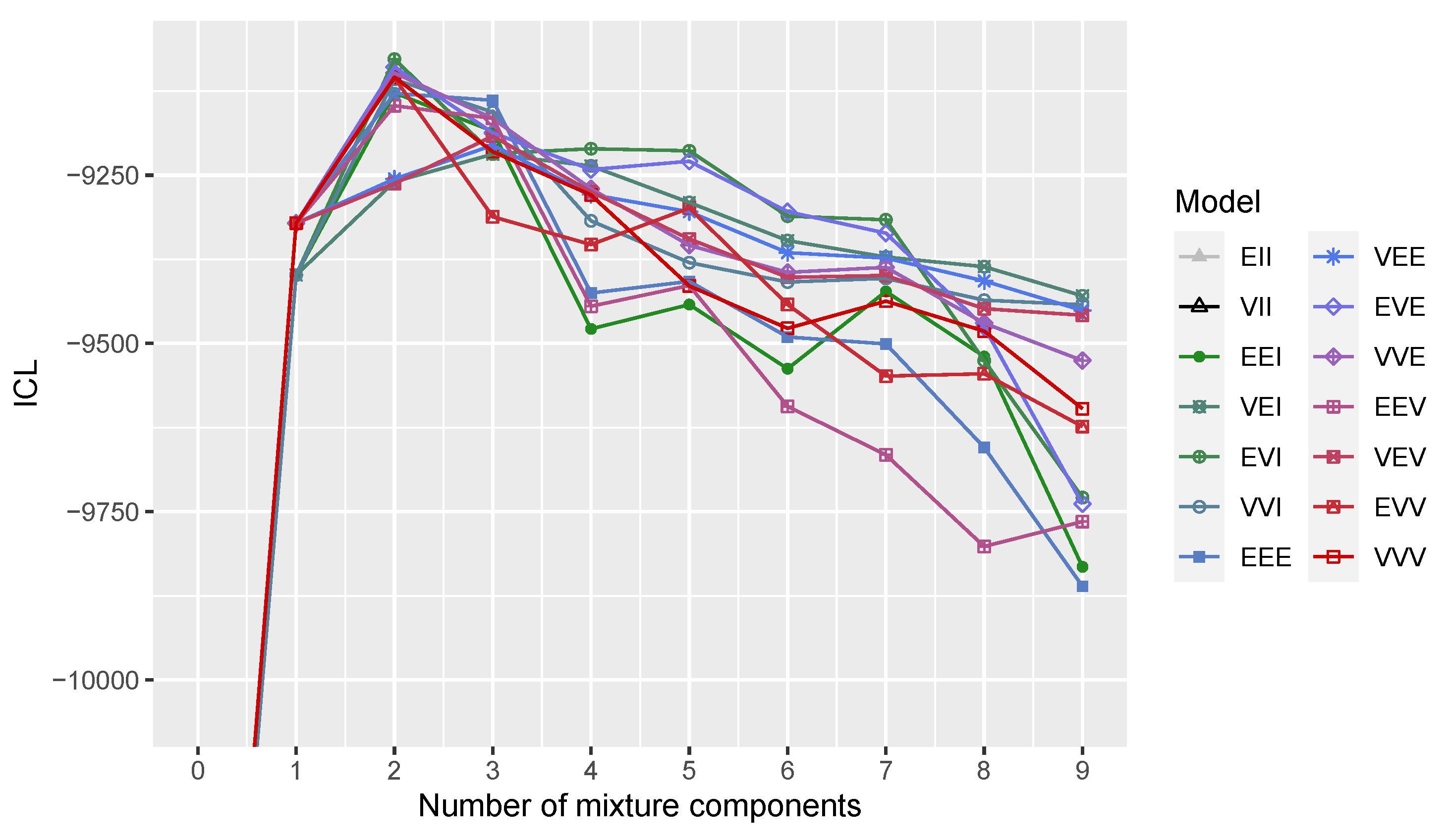
2.2. Model Selection

Given that a wide variety of GMMs in (1) can be estimated by varying the number of mixture components and the covariances’ decomposition in (2), selecting the appropriate model is a crucial matter. A popular option consists of choosing the “best” model using the Bayesian information criterion (BIC; [23]), which for a given model $\mathcal{M}$ is defined as

$${\mathrm{BIC}}_{\mathcal{M}}=2{\ell }_{\mathcal{M}}(\widehat{\mathit{\theta }})-{\nu }_{\mathcal{M}}log\left(n\right),$$

where ${\ell }_{\mathcal{M}}(\widehat{\mathit{\theta }})$ stands for the maximized log-likelihood of the data sample of size n under model $\mathcal{M}$ and ${\nu }_{\mathcal{M}}$ for the number of independent parameters to be estimated. Another available option in clustering is the Integrated Complete Likelihood (ICL; [24]) criterion given by

$${\mathrm{ICL}}_{\mathcal{M}}={\mathrm{BIC}}_{\mathcal{M}}+2\sum _{i=1}^n\sum _{k=1}^G{c}_{ik}log\left({\widehat{z}}_{ik}\right),$$

where ${\widehat{z}}_{ik}$ is the conditional probability that $x_i$ arises from the kth mixture component from Equation (4), and $c_{ik}=1$ if the ith observation is assigned to cluster ${\mathcal{C}}_k$ and 0 otherwise.

Both criteria evaluate the fit of a GMM to a given set of data by considering both the likelihood of the data given the model and the complexity of the model itself, represented by the number of parameters to be estimated. Compared to the BIC, the ICL introduces a further penalization for the overlap of the clusters. For this reason, the ICL tends to select models with well-separated clusters.

2.3. Including a Noise Component in Gaussian Mixtures

In the finite mixture framework, noisy data are characterized by the presence of outlying observations that do not belong to any mixture component. A strategy for accommodating noise is to include a uniform component with support in the convex hull of the data [7] resulting in the following mixture log-likelihood:

$$\ell (\mathit{\theta },{\pi }_0)=\sum _{i=1}^{n}log\left\{\frac{{\pi }_0}{V}+\sum _{k=1}^G{\pi }_k\varphi (x_i\mid {\mathit{\mu }}_k,{\mathsf{\Sigma }}_k)\right\},$$

(5)

where V is the hyper-volume of the data region and ${\pi }_0$ is the mixing weight associated with the noise component, with the mixing weights under the constraint ${\sum }_{k=0}^G{\pi }_k=1$. An observation contributes $V^{-1}$ to the likelihood if it belongs to the noise component; otherwise, its contribution comes from the Gaussian components.

The effectiveness of this approach hinges on obtaining an estimate of the hypervolume and a good initial specification of the noise to be used for starting the EM algorithm. The estimate of the hyper-volume can be computed using different approaches, such as the following:

• The volume of the convex hull, i.e., the smallest convex polygon that contains all the data points;
• The volume of the ellipsoid hull, i.e., the ellipsoid of minimal volume such that all observed points lie either inside or on the boundary of the ellipsoid;
• The volume computed as the minimum between the hyper-rectangle containing the observed data and the box obtained from principal components.

The first option would be the most accurate, but computing the convex hull of high-dimensional data can be challenging, as the number of vertices of the hull grows exponentially with the number of dimensions. The second option is computationally feasible even in high dimensions, but it is often inaccurate, as the volume of the ellipsoid hull can be significantly larger than the volume of the convex hull. A simple and fast approximation to the hyper-volume of the data can be computed using the last option. In fact, the hyper-rectangle is the simplest bounding box that can be used to enclose the data, while the box obtained from the principal components is a more sophisticated method that takes into account the shape and orientation of the data. By taking the minimum between these two volumes, an estimate of the volume of the convex hull can be obtained. Note that the function hypvol() of R package mclust uses this approach by default.

Regarding the initial denoising, some possible strategies include methods based on Voronoï tessellation [25], nearest neighbors [26], and robust covariance estimation [27]. In this paper we propose the use of data points’ contribution to the entropy of the estimated GMM to obtain an initial specification of noisy and outlying data points.

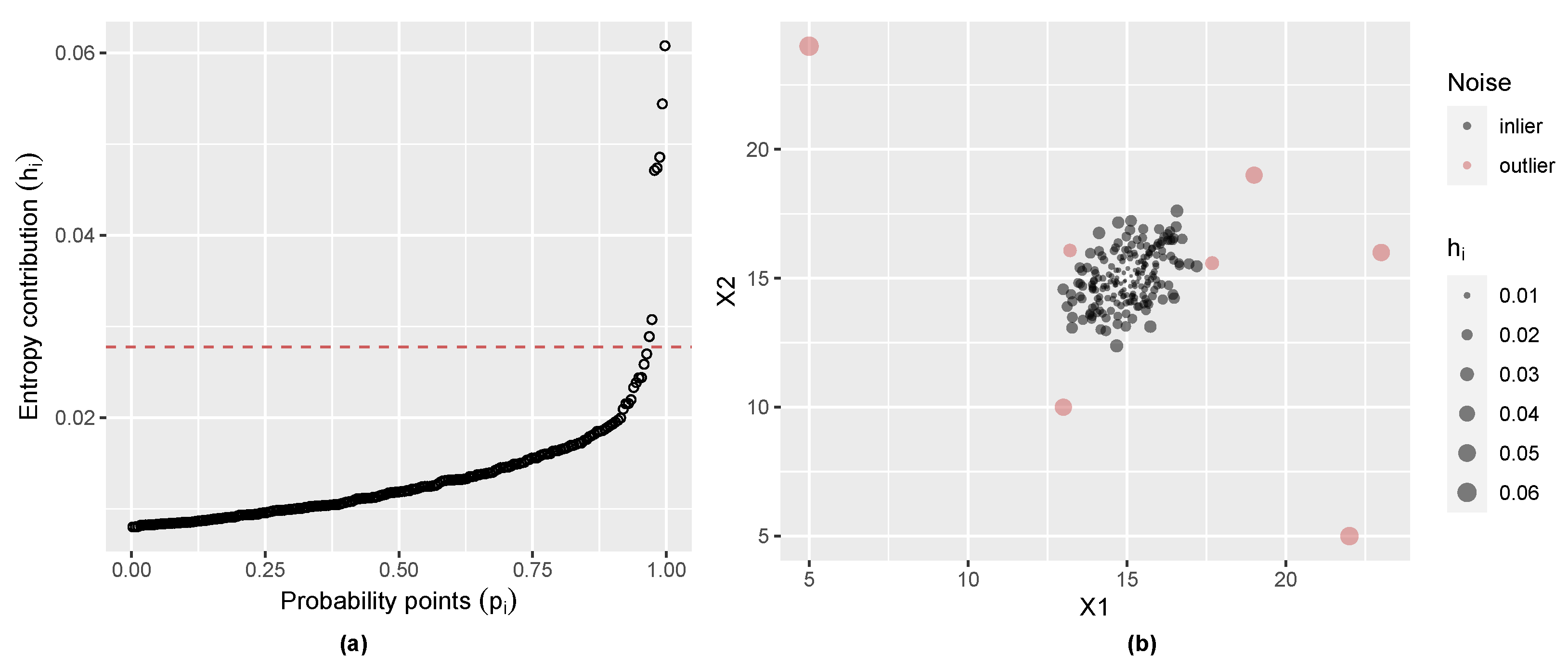
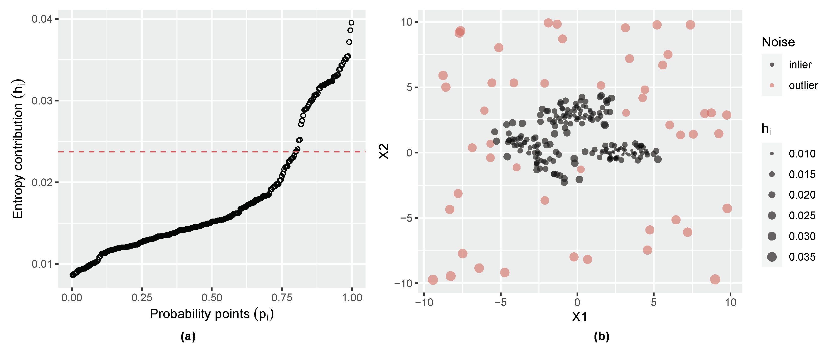
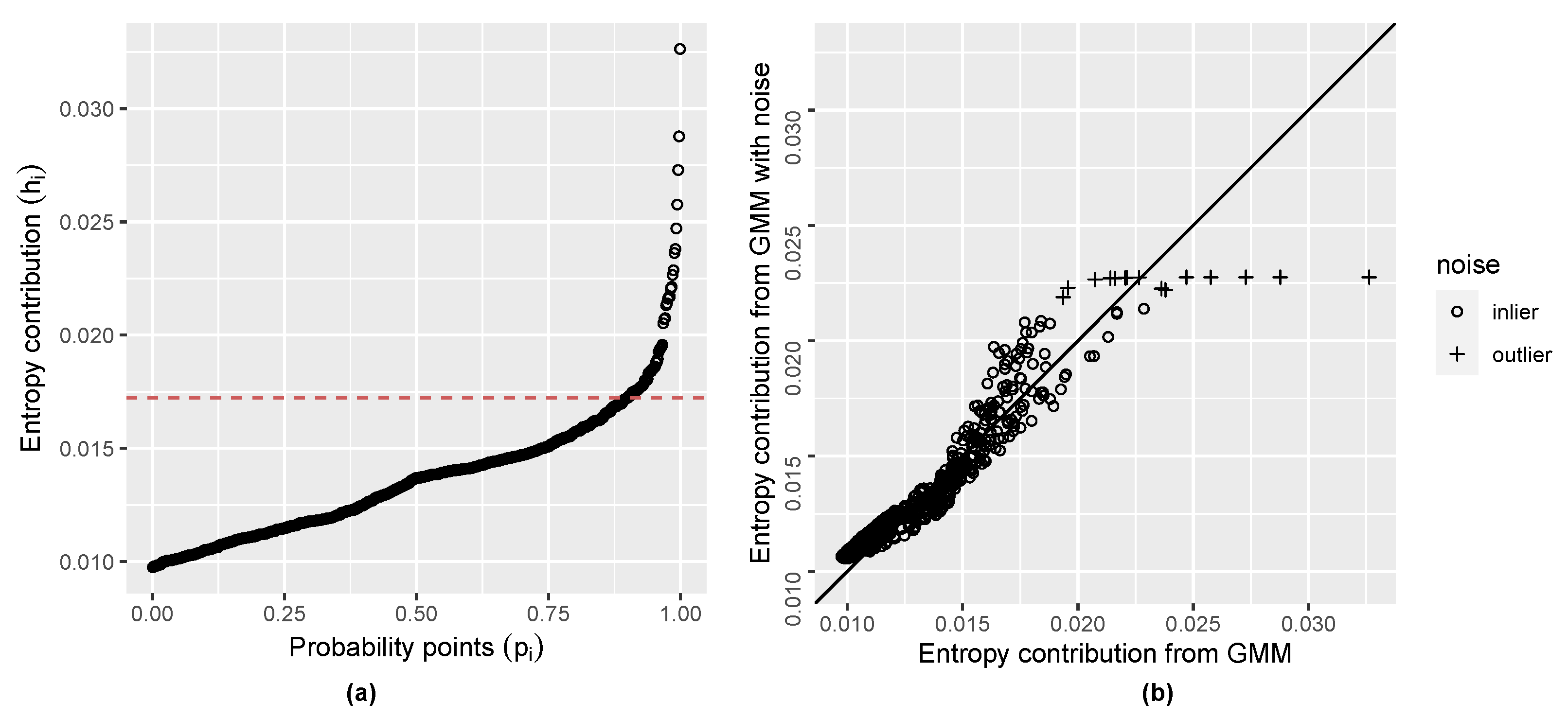
2.4. Initial Noise Detection Using Entropy Contribution of Data Points

Entropy is a measure of average uncertainty or information content in a random variable that plays a central role in information theory [28]. For a multivariate continuous random variable $X\in {\mathbb{R}}^d$ with probability density function $f\left(x\right)$, the entropy is defined as

$$H\left(X\right)=-{\int }_{\mathcal{X}}f\left(x\right)logf\left(x\right)\mathrm{d}x=-\mathbb{E}[logf\left(x\right)],$$

(6)

where $\mathcal{X}=\{x:f(x)>0\}$ is the support of the random variable [29].

A mixture-based estimate of the entropy has been recently proposed by Robin and Scrucca [30]. Assuming that the distribution of the multivariate random variable X can be expressed as a finite mixture of Gaussian components, the proposed estimate is easily obtained in practice using

$$\widehat{H}\left(X\right)=-\frac{1}{n}\sum _{i=1}^{n}log\widehat{f}(x_i;\widehat{\mathit{\theta }})=\sum _{i=1}^n{h}_i.$$

(7)

where $\widehat{f}(x_i;\widehat{\mathit{\theta }})$ is the mixture-based estimate of the density from Equation (1) with $\widehat{\mathit{\theta }}$ the MLE of the mixture parameters. Thus, an estimate of the entropy is obtained by summing over the contribution

$$h_i=-\frac{1}{n}log\widehat{f}(x_i;\widehat{\mathit{\theta }})$$

from each data point. This can also be interpreted as a measure of the degree of anomaly or outlierness of each observation.

A data-driven automatic procedure for selecting the initial outlying observations can be based on a comparison of the entropy contributions $h_i$, for $i=1,\dots ,n$, with those arising from a uniform distribution over the hyper-rectangle enclosing the data. Recalling that the entropy of a multivariate continuous uniform distribution is given by

$$H\left(U\right)=-{\int }_{{\mathcal{U}}_1}{\int }_{{\mathcal{U}}_2}\cdots {\int }_{{\mathcal{U}}_d}{V}^{-1}log\left(V^{-1}\right)\mathrm{d}{u}_1\mathrm{d}{u}_2\dots \mathrm{d}{u}_d=log\left(V\right).$$

Then, the contribution of each data point under the uniform distribution model can be computed as

$$u_i=log\left(V\right)/n\mathrm{for}\mathrm{all}i=1,\dots ,n.$$

A preliminary noise assignment is made by defining the set ${\tilde{\mathcal{C}}}_0=\{x_i:h_i>u_i\}$, with ${\tilde{n}}_0=\#\left\{{\tilde{\mathcal{C}}}_0\right\}$ giving the number of initial noisy data. The remaining $n-{\tilde{n}}_0$ observations are then partitioned using, for instance, model-based agglomerative clustering [31], to obtain ${\tilde{\mathcal{C}}}_k=\{x_i:h_i\le u_i\wedge x_i\in {\mathcal{P}}_k\}$, where ${\mathcal{P}}_k$ is the kth part of the partition with size ${\tilde{n}}_k=\#\left\{{\tilde{\mathcal{C}}}_k\right\}$ for $k=1,\dots ,G$, so that $n={\tilde{n}}_0+{\tilde{n}}_1+\cdots +{\tilde{n}}_G$. With this initial partition, the log-likelihood in (5) can be maximized using the EM algorithm. As a final result, the clusters ${\mathcal{C}}_1,\dots ,{\mathcal{C}}_G$ and the group of anomalies ${\mathcal{C}}_0$ are estimated, such that $\{{\mathcal{C}}_0\cup {\mathcal{C}}_1\cup \cdots \cup {\mathcal{C}}_G\}=\{x_1,x_2,\dots ,x_n\}$ and ${\mathcal{C}}_j\cap {\mathcal{C}}_k=\varnothing$ for $j\ne k$.

The general approach to anomaly detection proposed in this paper is summarized in Algorithm 1.

Algorithm 1: Anomaly detection algorithm

Input: Data matrix $X$ of n observations on d variables or features. Steps: Fit a GMM by maximizing the log-likelihood in (3) via the EM algorithm. Compute the contribution of each data point $h_i$ to the entropy. Select the initial noisy data by comparing the $h_i$ values with the reference values $u_i$ derived assuming a uniform distribution for the anomalies. Fit a GMM with the noise component by maximizing the log-likelihood in (5) via the EM algorithm. Output: Parameters estimate $({\widehat{\pi }}_0,{\widehat{\pi }}_1,\dots ,{\widehat{\pi }}_G,{\widehat{\mathit{\mu }}}_1,\dots ,{\widehat{\mathit{\mu }}}_G,{\widehat{\mathsf{\Sigma }}}_1,\dots ,{\widehat{\mathsf{\Sigma }}}_G)$; Probability for each data points to belong to one of the cluster or the noise component; Clustering partition $\mathcal{C}=\{{\mathcal{C}}_0,{\mathcal{C}}_1,\dots ,{\mathcal{C}}_G\}$.

3. Results

In this section, the proposed methodology for anomaly detection will be illustrated through examples utilizing both simulated and real datasets. The effectiveness of the approach will be showcased under controlled conditions through the use of simulated datasets and its practical utility in a real-world scenario will be discussed. Through these examples, the strengths of the approach and its ability to accurately detect anomalies in complex data will be highlighted.

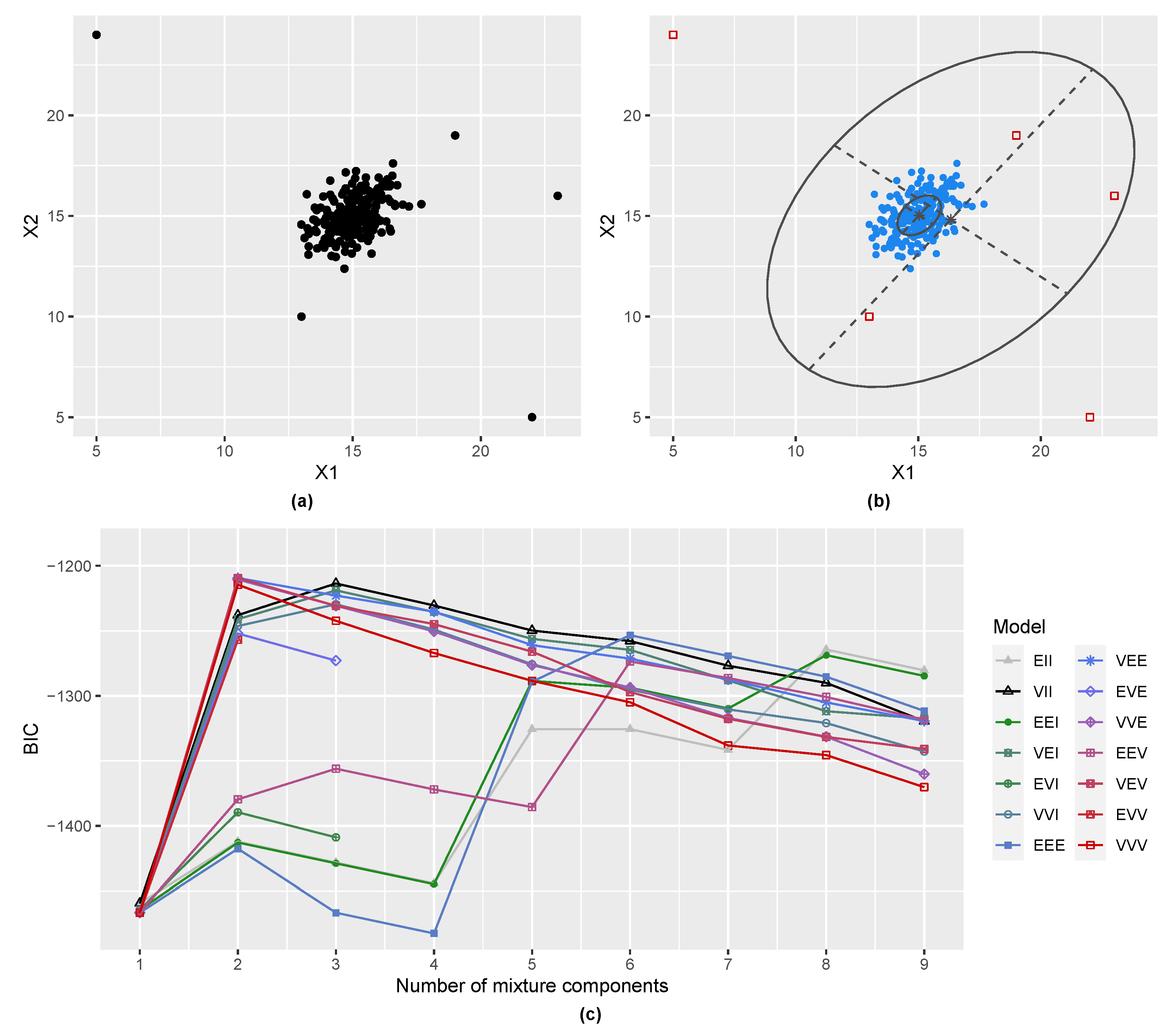
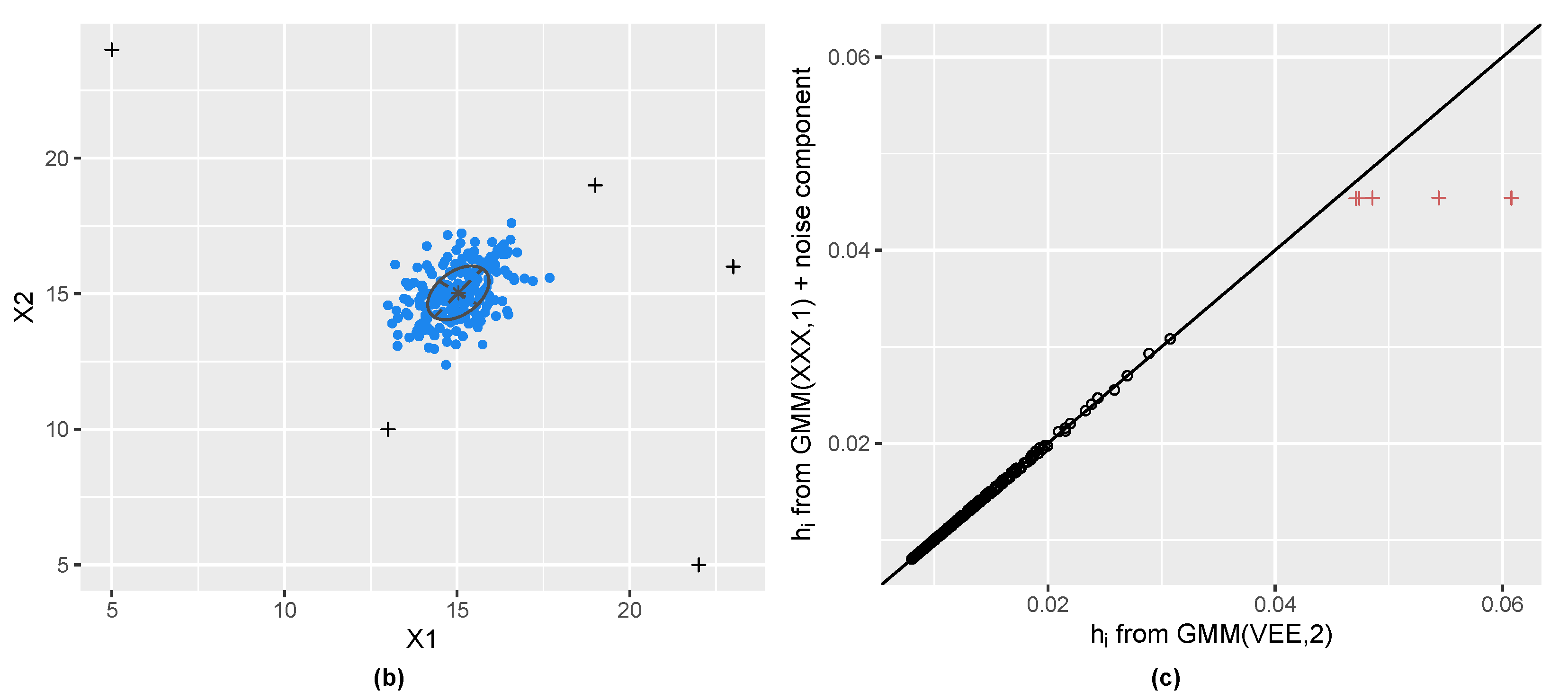
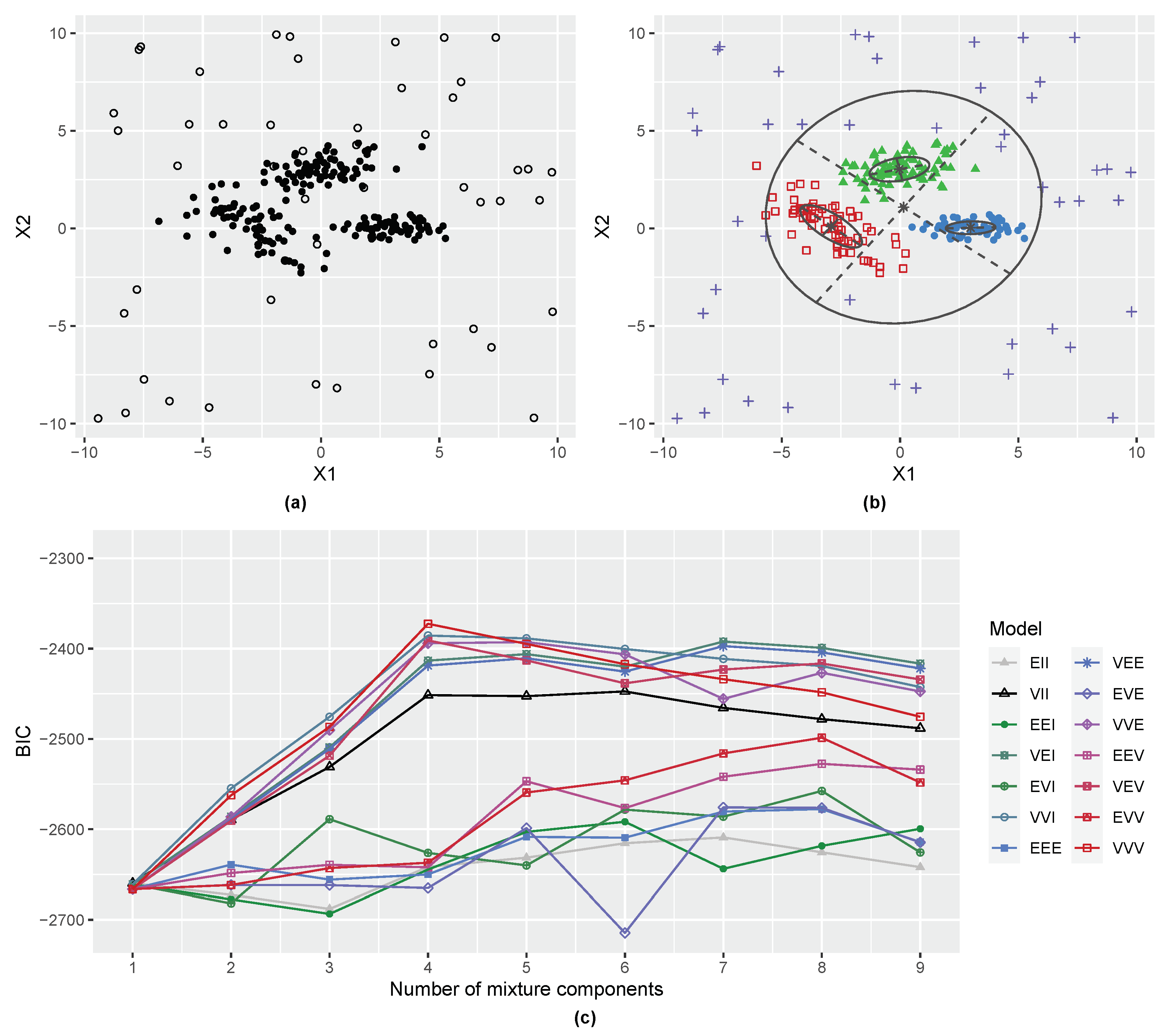
3.1. Gaussian Distribution with Outliers

Consider the dataset shown in Figure 1a generated from a bivariate Gaussian distribution with additional outliers added at the outskirts. According to the BIC criterion shown in Figure 1c, the optimal GMM estimated on this dataset is a two-component Gaussian mixture with covariance matrices having equal shape and orientation but different volume (VEE,2). Figure 1b shows the scatterplot with data points marked according to the GMM classification and the ellipses corresponding to the estimated cluster covariances. The presence of anomalies leads to the selection of a larger number of components, with an inflated covariance matrix for the second Gaussian component.

Figure 2a shows a plot of the entropy contribution values $h_i$ against the probability points $p_i=(i-0.5)/n$, for $i=1,\dots ,n$. Note that the $h_i$ values are sorted in non-decreasing order, which explains the increasing pattern observed in the graph. The dashed line refers to the entropy contribution from the uniform noise, so observations above that line can be included in the initial set of anomalies. Figure 2b shows a scatterplot with data points marked according to the initial classification of noise and with size proportional to the entropy contribution. It is easily seen that the points with the largest contribution are those far from the bulk of the data.

We then initialized the noise component using the identified data points as shown in Figure 2. The BIC traces in Figure 3a provide clear evidence that the data can be modeled using a single Gaussian component along with a noise component. Figure 3b confirms that the model successfully identifies the presence of a single Gaussian component despite the presence of some outliers in the data. A comparison of entropy contribution from the model without and the model with a noise component can be seen in Figure 3c. In the latter, the contribution from the outliers appears to flatten.

Finally, we note that for this simple case the anomaly detection procedure has both sensitivity and specificity equal to 1.

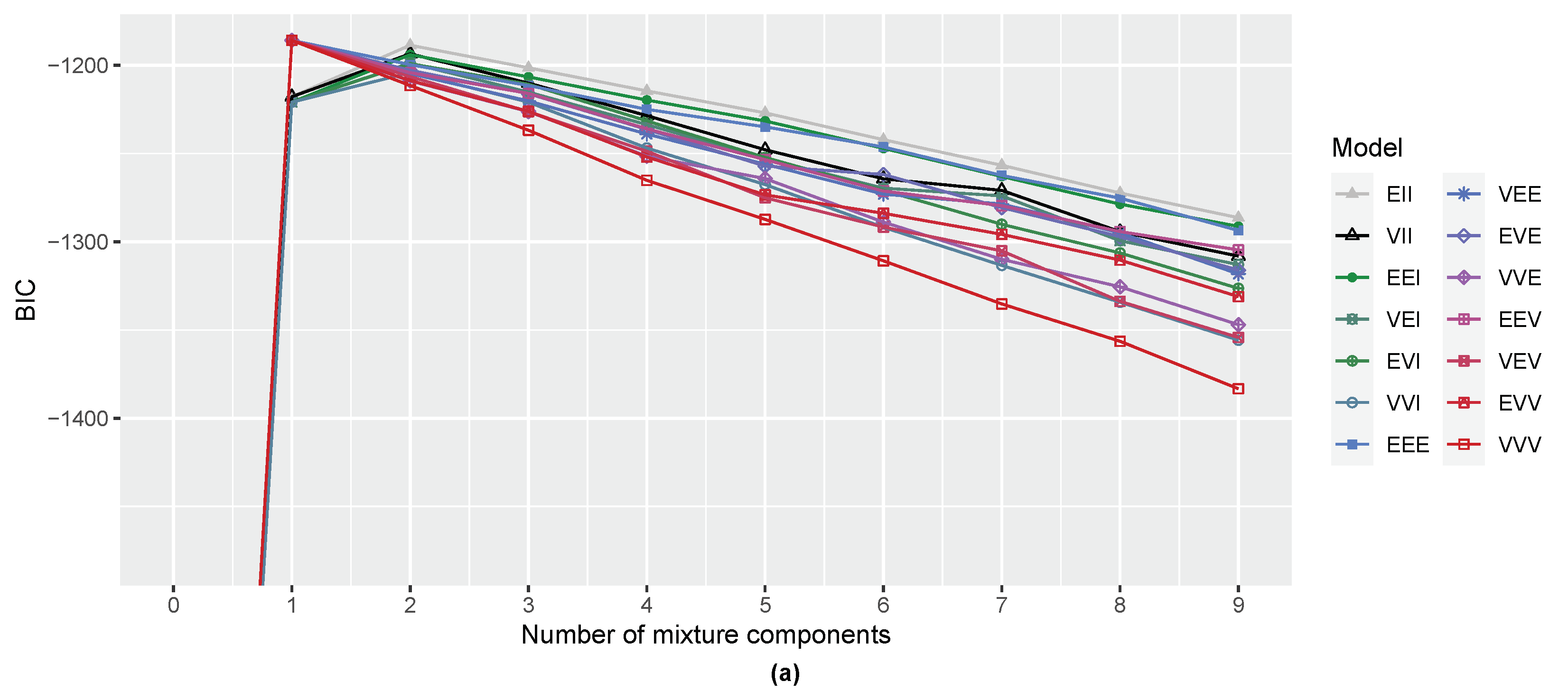
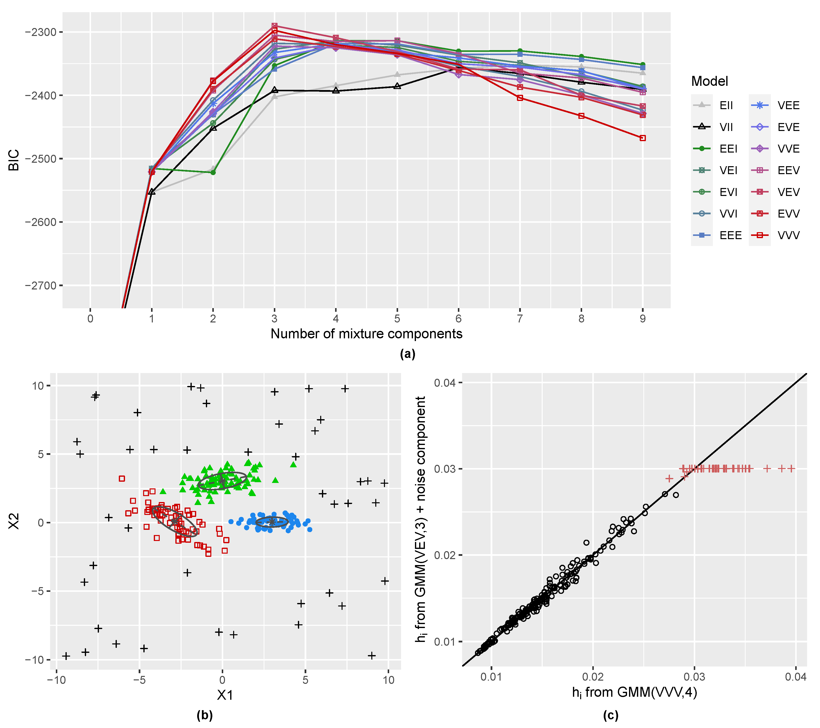
3.2. Three-Component Gaussian Mixture with Uniform Random Noise

In this second synthetic data example, a bivariate dataset is simulated from a three-component Gaussian mixture with equal mixing weights, different covariance matrices across components, and several noisy data points added from a uniform distribution over a square. The resulting dataset is shown in Figure 4a. The optimal GMM selected by BIC is a four-component Gaussian mixture with covariance matrices having varying volume, shape, and orientation (VVV,4; see Figure 4c). Figure 4b shows the scatterplot with data points marked according to the GMM classification and the ellipses corresponding to the estimated cluster covariances. A component with a large covariance is also necessary in this scenario to account for the noise present in the data.

Figure 5a contains the graph employed for the identification of the observations to be used in the initialization of the noise component, while the scatterplot in Figure 5b shows their distribution in the features space.

The optimal GMM with an additional component to account for anomalies is the three-component Gaussian mixture with covariance matrices having equal shape but varying volume and orientation (VEV,3; see Figure 6a). Figure 6b shows the scatterplot with data points marked according to the GMM classification (including the noise component). As a result, most of the simulated outliers are identified by the final model. Finally, a comparison of the entropy contribution from the model without and the model with a noise component can be seen in Figure 6c. From this graph it can be seen that the contribution to the overall entropy is mostly reduced for the observations assigned to the noise component.

Finally, we note that for this dataset the anomaly detection procedure has sensitivity equal to 0.84 and specificity 0.99. Thus, the procedure appears to be quite goood at distinguishing normal data from anomalous data without mistakenly flagging normal data as anomalous.

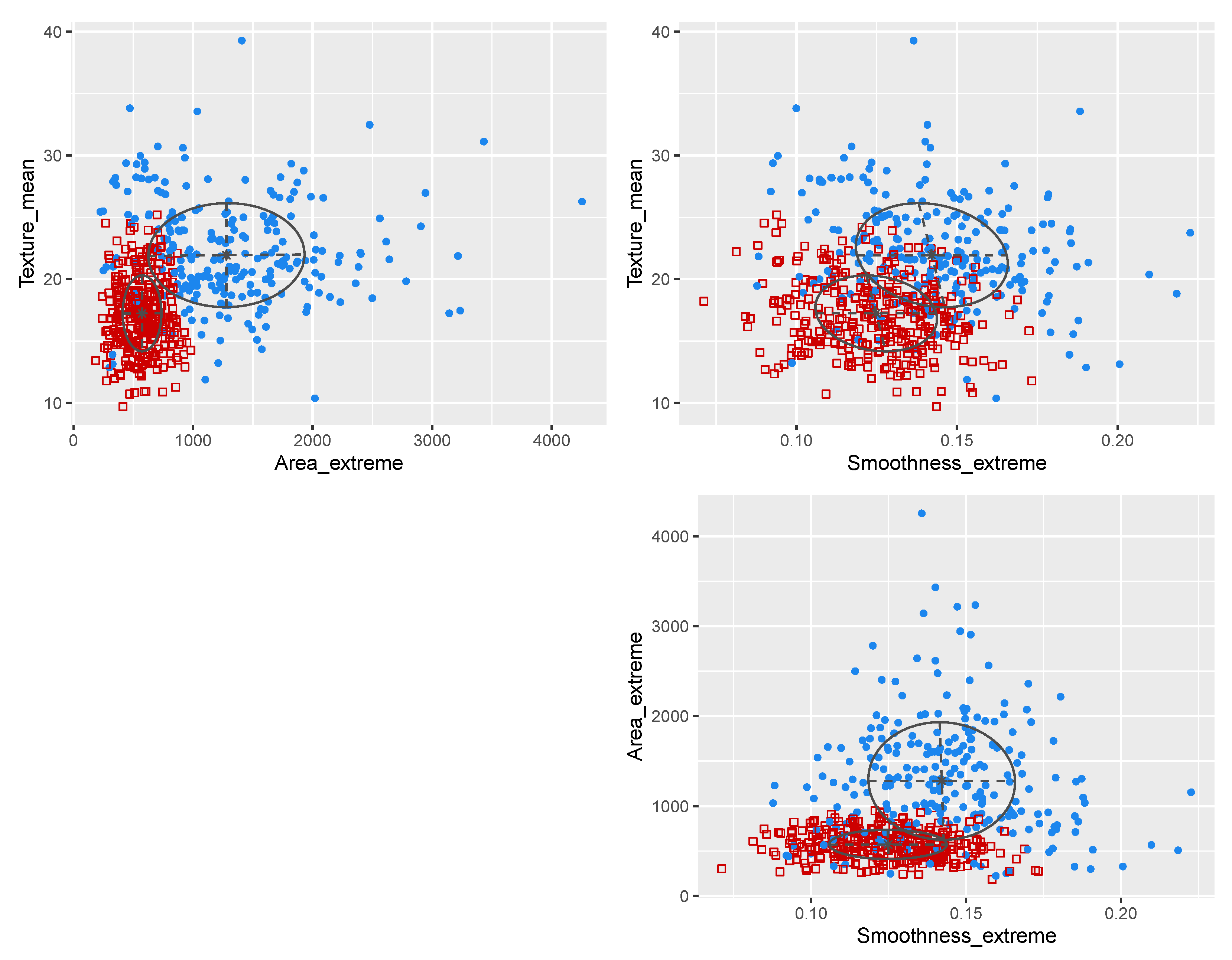
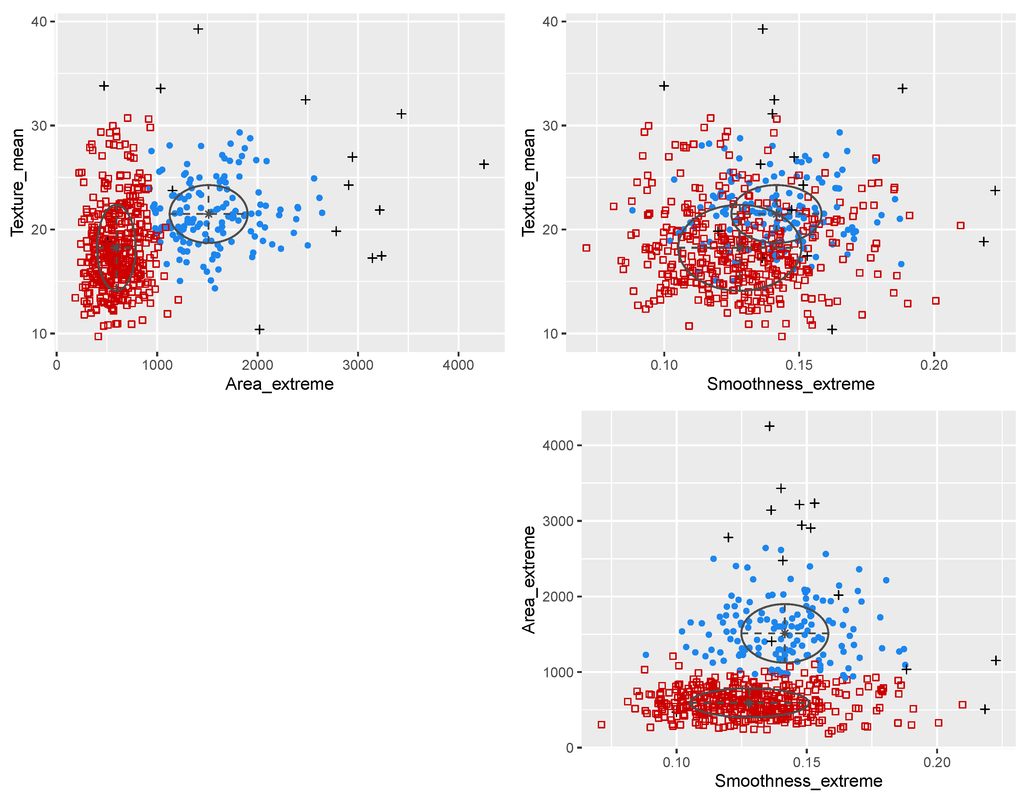
3.3. Wisconsin Diagnostic Breast Cancer Data

This dataset, available at the UCI Machine Learning Repository [32], contains measurements for 569 patients on 30 features of the cell nuclei obtained from a digitized image of a fine needle aspirate (FNA) of a breast mass Mangasarian et al. [33]. Each patient’s breast mass was later analyzed and classified as either malignant (212 cases) or benign (357 cases). In accordance with Mangasarian et al. [33] and Fraley and Raftery [15], we rely on three features for clustering: extreme area, extreme smoothness, and mean texture. Furthermore, the following analysis does not assume knowledge of either the covariance eigen-decomposition or the number of mixture components.

We start our analysis by fitting several GMMs with all the available eigen-decomposition of covariance matrices and with number of mixture components from 1 to 9. The “optimal” model is selected using ICL, as described in Section 2.2, with ICL traces shown in Figure 7. Based on this criterion, we selected the VVE model with 2 clusters.

Table 1. Summary and clustering results provided by mclust package for the model GMM(VVE,2) estimated on the Wisconsin diagnostic breast cancer data.

----------------------------------------------------
Gaussian finite mixture model fitted by EM algorithm
----------------------------------------------------
Mclust VVE (ellipsoidal, equal orientation) model with 2 components:
log-likelihood					n	df	BIC	ICL	Entropy
−4449.632					569	16	−9000.766	−9099.815	7.820091
Clustering table:
1	2
240	329
Confusion matrix:
Cluster
Diagnosis			1	2
B			40	317
M			200	12

provides a summary and clustering results for the estimated model.

Figure 8 shows the scatterplots between pairs of features with data points marked according to the estimated clusters from model (VVE,2) and corresponding ellipses representing estimated cluster covariances. There is clearly a strong overlap between the two groups, which roughly represent the two types of diagnoses. Note that some data points from one group are located around the majority of data points from the other group. This is the consequence of an inflated covariance matrix. One further characteristic that emerges from the plots in Figure 8 is the presence of many data points that are distant from the bulk of the data, particularly for the malignant cases.

Figure 9a shows the contribution of each case to the overall entropy, with the reference dashed line representing the entropy contribution from the uniform noise. Using the observations above the uniform-noise reference line for initialization of the noise component, and the default estimate of the volume of the data, GMMs with an additional component for the noise can be estimated. A summary of the “optimal” model according to ICL is reported in

Table 2. Summary and clustering results for the model GMM(EVI,2) with the noise component estimated on the Wisconsin diagnostic breast cancer data.

----------------------------------------------------
Gaussian finite mixture model fitted by EM algorithm
----------------------------------------------------
Mclust EVI (diagonal, equal volume, varying shape) model with 2 components and a noise term:
log-likelihood				n	df	BIC	ICL	Entropy
−4457.913				569	14	−9004.64	−9077.593	7.834645
Clustering table:
1	2	0
142	412	15
Confusion matrix:
Cluster
Diagnosis noise				1	2
B			1	0	356
M			14	142	56

, while Figure 10 shows the ICL traces that lead to the selection of model GMM(EVI,2).

Figure 11 shows the scatterplots between pairs of features with data points marked according to the classification provided by the GMM with the noise component reported in Table 2, and ellipses corresponding to the estimated cluster covariances. Data points drawn with the + symbol represent the detected outliers. According to the Maximum a Posteriori (MAP) principle, these are classified as belonging to the noise component due to their highest posterior conditional probabilities compared to the probabilities of belonging to any of the Gaussian components. Note that the two clusters identified by this model appear to be more clearly separated than in Figure 8. Almost all malignant cases are included in the first cluster, which presents the characteristic of having Area_extreme $>1000$. Outliers clearly appear to be located around the edge of the two main groups. Moreover, except for one instance, all the cases belong to the malignant class, suggesting that diseased tissues are more likely to result in abnormal values.

4. Conclusions

In this paper, we presented a novel approach to the initial specification of the noise component in a Gaussian mixture model, offering a new and effective methodology for the challenging problem of anomaly detection. Our proposed approach involves an automatic procedure for selecting the initial outlying observations to be used in the EM algorithm for Gaussian mixture models with a noise component. Specifically, the initialization of the noise is based on a comparison of the contribution of each data point to the entropy of the Gaussian mixture with the contribution arising from a uniform distribution over the hyper-rectangle that encloses the data.

We demonstrated the effectiveness of our proposal by successfully identifying anomalies in both simulated and real-world datasets, even in the presence of significant levels of noise and outliers. However, there is still much room for improvement and future research in this area. A comprehensive comparison with other state-of-the-art methods would be valuable for evaluating the effectiveness of our proposal. Another promising avenue for future research is to expand the scope of our study by using simulated data from a broad parameter landscape. This would allow for the investigation of the sensitivity and specificity of the procedure under a wider range of conditions and the identification of areas where further improvements are needed. In particular, close attention should be devoted to the specificity of the procedure, which is a critical measure of its performance in distinguishing normal data from anomalous data without mistakenly flagging normal data as anomalous.

Finally, we mentioned that our proposal is applicable to a wide range of applications, making it a valuable contribution to the field of anomaly detection using Gaussian mixture models. Overall, this paper can help advance the state of the art in robust and effective anomaly detection, and it will be of interest to researchers and practitioners working in this field.

References

1. McLachlan, G.J.; Peel, D. Finite Mixture Models; Wiley: New York, NY, USA, 2000. [Google Scholar]
2. Yeung, K.Y.; Fraley, C.; Murua, A.; Raftery, A.E.; Ruzzo, W.L. Model-based clustering and data transformations for gene expression data. Bioinformatics 2001, 17, 977–987. [Google Scholar] [CrossRef] [PubMed] [Green Version]
3. McLachlan, G.; Bean, R.; Peel, D. A mixture model-based approach to the clustering of microarray expression data. Bioinformatics 2002, 18, 413–422. [Google Scholar] [CrossRef] [PubMed] [Green Version]
4. Najarian, K.; Zaheri, M.; Rad, A.A.; Najarian, S.; Dargahi, J. A novel mixture model method for identification of differentially expressed genes from DNA microarray data. BMC Bioinform. 2004, 5, 201. [Google Scholar] [CrossRef] [PubMed] [Green Version]
5. Ko, Y.; Zhai, C.; Rodriguez-Zas, S.L. Inference of gene pathways using Gaussian mixture models. In Proceedings of the 2007 IEEE International Conference on Bioinformatics and Biomedicine (BIBM 2007), Fremont, CA, USA, 2–4 November 2007; pp. 362–367. [Google Scholar] [CrossRef]
6. Hirsch, M.; Habeck, M. Mixture models for protein structure ensembles. Bioinformatics 2008, 24, 2184–2192. [Google Scholar] [CrossRef] [Green Version]
7. Dasgupta, A.; Raftery, A.E. Detecting features in spatial point processes with clutter via model-based clustering. J. Am. Stat. Assoc. 1998, 93, 294–302. [Google Scholar] [CrossRef]
8. Fraley, C.; Raftery, A.E. How many clusters? Which clustering method? Answers via model-based cluster analysis. Comput. J. 1998, 41, 578–588. [Google Scholar] [CrossRef]
9. Coretto, P.; Hennig, C. Robust improper maximum likelihood: Tuning, computation, and a comparison with other methods for robust Gaussian clustering. J. Am. Stat. Assoc. 2016, 111, 1648–1659. [Google Scholar] [CrossRef]
10. Dang, U.J.; Browne, R.P.; McNicholas, P.D. Mixtures of multivariate power exponential distributions. Biometrics 2015, 71, 1081–1089. [Google Scholar] [CrossRef] [Green Version]
11. Punzo, A.; McNicholas, P.D. Parsimonious mixtures of multivariate contaminated normal distributions. Biom. J. 2016, 58, 1506–1537. [Google Scholar] [CrossRef] [Green Version]
12. García-Escudero, L.A.; Gordaliza, A.; Matràn, C.; Mayo-Iscar, A. A general trimming approach to robust cluster analysis. Ann. Stat. 2008, 36, 1324–1345. [Google Scholar] [CrossRef]
13. Dotto, F.; Farcomeni, A. Robust inference for parsimonious model-based clustering. J. Stat. Comput. Simul. 2019, 89, 414–442. [Google Scholar] [CrossRef] [Green Version]
14. Farcomeni, A.; Punzo, A. Robust model-based clustering with mild and gross outliers. TEST 2020, 29, 989–1007. [Google Scholar] [CrossRef]
15. Fraley, C.; Raftery, A.E. Model-based clustering, discriminant analysis, and density estimation. J. Am. Stat. Assoc. 2002, 97, 611–631. [Google Scholar] [CrossRef]
16. Banfield, J.; Raftery, A.E. Model-based Gaussian and non-Gaussian clustering. Biometrics 1993, 49, 803–821. [Google Scholar] [CrossRef]
17. Celeux, G.; Govaert, G. Gaussian parsimonious clustering models. Pattern Recognit. 1995, 28, 781–793. [Google Scholar] [CrossRef] [Green Version]
18. R Core Team. R: A Language and Environment for Statistical Computing; R Foundation for Statistical Computing: Vienna, Austria, 2022. [Google Scholar]
19. Fraley, C.; Raftery, A.E.; Scrucca, L. mclust: Gaussian Mixture Modelling for Model-Based Clustering, Classification, and Density Estimation; R Package Version 6.0.0; R Foundation for Statistical Computing: Vienna, Austria, 2022. [Google Scholar]
20. Scrucca, L.; Fop, M.; Murphy, T.B.; Raftery, A.E. mclust 5: Clustering, classification and density estimation using Gaussian finite mixture models. R J. 2016, 8, 205–233. [Google Scholar] [CrossRef] [Green Version]
21. Dempster, A.P.; Laird, N.M.; Rubin, D.B. Maximum likelihood from incomplete data via the EM algorithm (with discussion). J. R. Stat. Soc. Ser. B Stat. Methodol. 1977, 39, 1–38. [Google Scholar]
22. McLachlan, G.; Krishnan, T. The EM Algorithm and Extensions, 2nd ed.; Wiley-Interscience: Hoboken, NJ, USA, 2008. [Google Scholar]
23. Schwarz, G. Estimating the dimension of a model. Ann. Stat. 1978, 6, 461–464. [Google Scholar] [CrossRef]
24. Biernacki, C.; Celeux, G.; Govaert, G. Assessing a mixture model for clustering with the integrated completed likelihood. IEEE Trans. Pattern Anal. Mach. Intell. 2000, 22, 719–725. [Google Scholar] [CrossRef]
25. Allard, D.; Fraley, C. Nonparametric maximum likelihood estimation of features in spatial point processes using Voronoï tessellation. J. Am. Stat. Assoc. 1997, 92, 1485–1493. [Google Scholar] [CrossRef]
26. Byers, S.; Raftery, A.E. Nearest-neighbor clutter removal for estimating features in spatial point processes. J. Am. Stat. Assoc. 1998, 93, 577–584. [Google Scholar] [CrossRef]
27. Wang, N.; Raftery, A.E. Nearest neighbor variance estimation (NNVE): Robust covariance estimation via nearest neighbor cleaning (with discussion). J. Am. Stat. Assoc. 2002, 97, 994–1019. [Google Scholar] [CrossRef]
28. Cover, T.M.; Thomas, J.A. Elements of Information Theory, 2nd ed.; John Wiley & Sons: Hoboken, NJ, USA, 2006. [Google Scholar]
29. Michalowicz, J.V.; Nichols, J.M.; Bucholtz, F. Handbook of Differential Entropy; Chapman & Hall/CRC: Boca Raton, FL, USA, 2014. [Google Scholar]
30. Robin, S.; Scrucca, L. Mixture-based estimation of entropy. Comput. Stat. Data Anal. 2023, 177, 107582. [Google Scholar] [CrossRef]
31. Fraley, C. Algorithms for model-based Gaussian hierarchical clustering. SIAM J. Sci. Comput. 1998, 20, 270–281. [Google Scholar] [CrossRef] [Green Version]
32. Dua, D.; Graff, C. UCI Machine Learning Repository. 2019. Available online: http://archive.ics.uci.edu/ml (accessed on 15 January 2023).
33. Mangasarian, O.L.; Street, W.N.; Wolberg, W.H. Breast cancer diagnosis and prognosis via linear programming. Oper. Res. 1995, 43, 570–577. [Google Scholar] [CrossRef] [Green Version]
Figure 1. Scatterplot of first synthetic data example with data points generated from a Gaussian distribution with outliers at the outskirts (a). Estimated GMM with points marked by colors and symbols according to the GMM classification, ellipses corresponding to estimated cluster covariances, dashed lines referring to principal axes, and ∗ to the cluster means (b). BIC traces for the selection of the optimal GMM model (c).
Algorithms 16 00195 g001
Figure 2. Entropy contribution of each data point in the first synthetic dataset, with dashed horizontal line from uniform noise for reference (a). Scatterplot of data points marked according to the initial classification of noise and with size proportional to the entropy contribution (b).
Algorithms 16 00195 g002
Figure 3. BIC traces for the selection of the optimal GMM with the noise component on the first synthetic data example (a). Scatterplot of data points marked by colors and symbols according to the classification (identified anomalies are represented with the + symbol) from the estimated GMM with the noise component, ellipse corresponding to estimated cluster covariance, dashed lines referring to principal axes, and ∗ to the cluster means (b). Plot of entropy contribution values h i for the model without and with the noise component (c).
Algorithms 16 00195 g003aAlgorithms 16 00195 g003b
Figure 4. Scatterplot of second synthetic data example with data points generated from a three-component Gaussian mixture with equal mixing weights and different covariance matrices across components (represented with the • symbol), and with several noise data points added from a uniform distribution over a square (represented with the ∘ symbol) (a). Estimated GMM with points marked by colors and symbols according to the GMM classification, ellipses corresponding to estimated cluster covariances, dashed lines referring to principal axes, and ∗ to the cluster means (b). BIC traces for the selection of the optimal GMM (c).
Algorithms 16 00195 g004
Figure 5. Entropy contribution of each data point in the second synthetic dataset, with dashed horizontal line from uniform noise for reference (a). Scatterplot of data points marked according to the initial classification of noise and with size proportional to the entropy contribution (b).
Algorithms 16 00195 g005
Figure 6. BIC traces for the selection of the optimal GMM with the noise component on the second synthetic data example (a). Scatterplot of data points marked by colors and symbols according to the classification (identified anomalies are represented with the + symbol) from the estimated GMM with the noise component, ellipse corresponding to estimated cluster covariance, dashed lines referring to principal axes, and ∗ to the cluster means (b). Plot of entropy contribution values h i for the model without and with the noise component (c).
Algorithms 16 00195 g006
Figure 7. ICL traces from fitting GMMs without the noise component to the Wisconsin diagnostic breast cancer data.
Algorithms 16 00195 g007
Figure 8. Scatterplots of selected features for the Wisconsin diagnostic breast cancer data with data points marked according to the GMM(VVE,2) classification and ellipses representing estimated cluster covariances. Data points represented by are assigned to the cluster predominantly composed of malignant cases, while those represented by refers to the cluster mainly composed of benign cases.
Algorithms 16 00195 g008
Figure 9. Entropy contribution of each data point in the Wisconsin diagnostic breast cancer data, with dashed horizontal line from uniform noise for reference (a). Plot of entropy contribution values h i for the model without and with the noise component (b).
Algorithms 16 00195 g009
Figure 10. ICL traces from fitting GMMs with the noise component for the Wisconsin diagnostic breast cancer data.
Algorithms 16 00195 g010
Figure 11. Scatterplots of selected features for the Wisconsin diagnostic breast cancer data with data points marked according to the classification from the GMM(EVI,2) with the noise component model and ellipses representing estimated cluster covariances. The 1st cluster is represented using the symbol and it is made by all malignant cases, while the 2nd cluster is represented using the symbol and it is mainly composed by benign cases. Finally, data points classified as noise are represented using a + symbol.
Algorithms 16 00195 g011