Article

A Bioinformatics Analysis of Ovarian Cancer Data Using Machine Learning

1
Department of Engineering and Natural Sciences, Technical University of Applied Sciences Wildau, 15745 Wildau, Germany
2
Department of Biochemistry and Molecular Medicine, University of California, Davis, CA 95817, USA
3
Ibiomics UG, 14193 Berlin, Germany
*
Authors to whom correspondence should be addressed.
Algorithms 2023, 16(7), 330; https://doi.org/10.3390/a16070330
Submission received: 30 April 2023 / Revised: 6 July 2023 / Accepted: 7 July 2023 / Published: 11 July 2023
(This article belongs to the Special Issue Machine Learning Algorithms for Bioinformatics Problems)

Abstract

:
The identification of biomarkers is crucial for cancer diagnosis, understanding the underlying biological mechanisms, and developing targeted therapies. In this study, we propose a machine learning approach to predict ovarian cancer patients’ outcomes and platinum resistance status using publicly available gene expression data. Six classical machine-learning algorithms are compared on their predictive performance. Those with the highest score are analyzed by their feature importance using the SHAP algorithm. We were able to select multiple genes that correlated with the outcome and platinum resistance status of the patients and validated those using Kaplan–Meier plots. In comparison to similar approaches, the performance of the models was higher, and different genes using feature importance analysis were identified. The most promising identified genes that could be used as biomarkers are TMEFF2, ACSM3, SLC4A1, and ALDH4A1.

1. Introduction

Ovarian cancer is the most lethal gynecologic malignancy, with a five-year survival rate of 49% for all stages of the cancer [1]. Ovarian cancer is very aggressive and often recurs after subsequent treatments. Most patients will acquire resistance through treatment consisting of carboplatin-based chemotherapy as well as PARP inhibitors [2,3].
Ovarian cancer is frequently diagnosed at advanced FIGO stages, which leads to overall poor survival rates. The symptoms are generally non-specific, and therefore early detection methods, genetic screening, and multiple treatment options are needed to improve the outcomes of patients with ovarian cancer [4,5].
Recent studies have demonstrated that biological parameters like mRNA gene expression can be linked to and predict the outcome of cancer patients [6,7,8]. For that matter, statistical methods have been used, as well as machine learning methods [9]. Studies have shown that machine learning models achieve high performance in predicting potential biomarkers, the stage of cancer, platinum sensitivity, relapse time, as well as overall survival (OS) in ovarian cancer using gene expression profiles, image data, copy number variations, and more [10,11,12,13,14].
In a previous study by Spentzos et al. [15], the SPLASH algorithm was used for the initial discovery of candidate biomarkers from mRNA gene expression analysis and weighted voting and k nearest neighbor for training and leave-one-out cross-validation for predictive accuracy. In another study by Hartmann et al. [11], a supervised machine-learning approach using the support vector machine algorithm was applied to mRNA gene expression to identify biomarkers associated with early recurrences in ovarian cancer. Yang et al. [16] used microRNA expression data and differential gene expression analysis between a complete response and noncomplete response to identify miRNAs differentially associated with clinical response to chemotherapy.
In previous studies by the Cancer Genome Atlas Research Network [17], a univariate Cox regression model was used to identify 193-genes signature predictive of overall survival in high-grade serous ovarian cancer, and this model was refined to 100-genes signature in subsequent studies [18] using ssGSEA scores of tumor samples from multiple independent gene expression data sets and a multiple covariate model that includes molecular subtypes.
Millstein et al. [12] used the Cox proportional hazards regression adjusted for molecular subtype from six microarray gene expression studies, totaling 1455 participants, and identified 200 candidate genes. They included additional 313 genes based on the literature and published data, and candidate gene expression was determined by Nanostring in 4071 samples from 16 studies and selected elastic net regularized regression model from evaluated four models for further training and validation to arrive at 101-genes prognostic signature. Finally, in Zhang et al. [19] studies, a network-based Cox proportional hazard model was applied to three independent data sets to identify biomarkers associated with patient outcomes in ovarian cancer.
In this study, we use differential gene expression analysis to identify initial biomarkers associated with outcome and apply SHAP (Shapley additive explanations) algorithm for feature extraction, which has so far been used only once in ovarian cancer data for platinum sensitivity and to our knowledge, not on outcome prediction [20,21]. We analyze one of the largest publicly available gene expression data sets for ovarian cancer to predict the outcome of patients with ovarian cancer and find candidate biomarkers associated with differential outcomes or responses to chemotherapy. Figure 1 provides an overview of the structure of the approach. A combination of bioinformatics analysis and machine learning methods is used to identify relationships between biological components, disease progression, and patient outcomes.

2. Materials and Methods

2.1. Materials

The data from the Cancer Genome Atlas (TCGA) [17,22] are used in this study. They consist of 585 ovarian cancer patients. The unnormalized gene expression counts from the mRNA sequencing data from National Cancer Institute Genomic Data Common (GDC) are used for differential gene expression analysis with DESeq2 [23]. The clinical data of the patients are used for good or bad outcomes and platinum resistance or sensitive classifications.
The outcome and platinum response status were not available for some patients in this study. To address this, two approaches were taken. In the first approach, patients were filtered based on the availability of mRNA sequencing data and their classification as either having a good or bad outcome. In the second approach, patients were required to have both mRNA sequencing data and platinum response status available. After filtering, the remaining patient data were randomly divided into training, testing, and independent validation datasets. The training dataset was utilized to train the machine learning models, whereas the testing dataset was used to test the performance of these models in multiple trials. Finally, the validation dataset was employed to evaluate the performance of the models on data that were not previously used for training or testing.

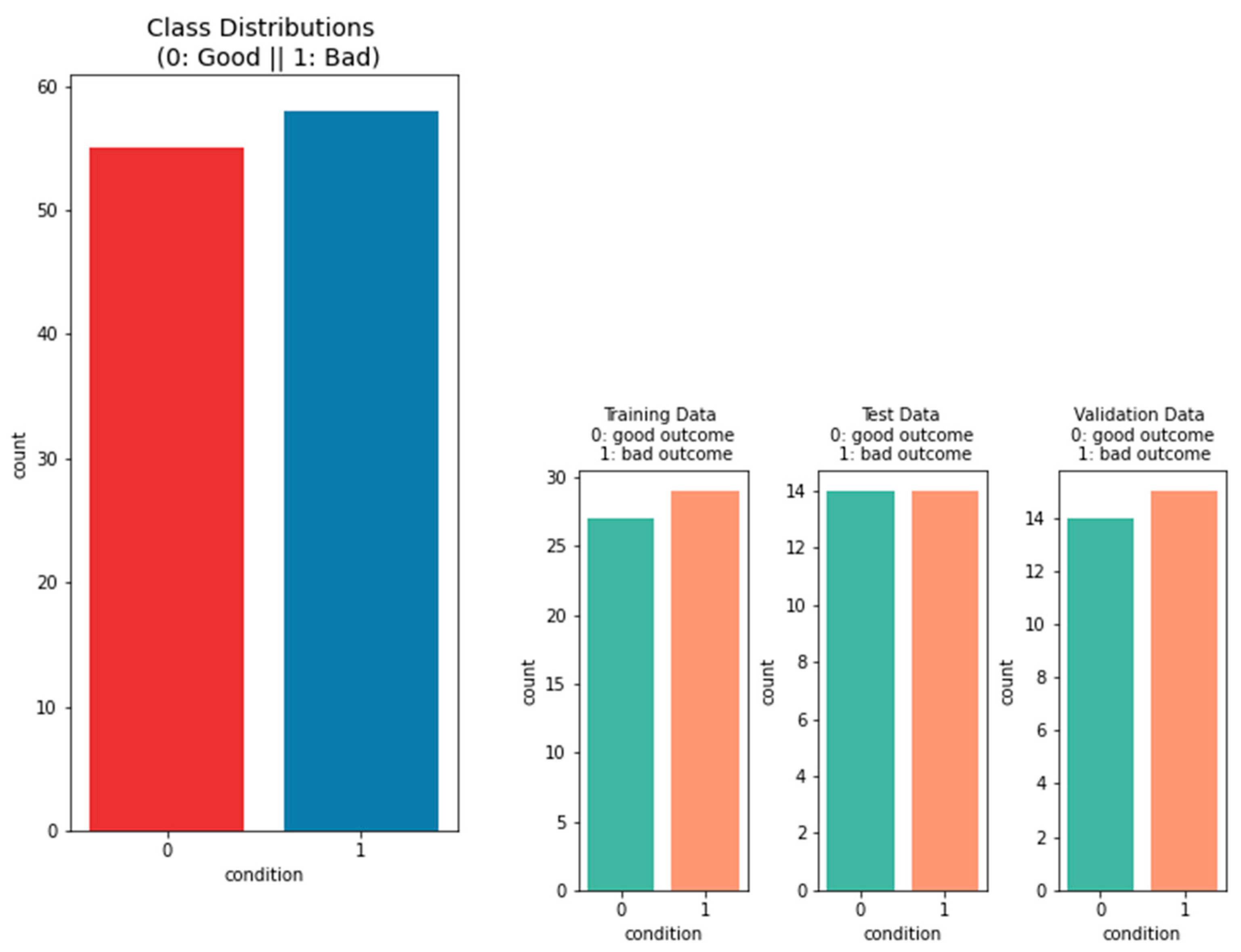
2.1.1. Data on the Outcome of the Patients

To identify potential biomarkers for ovarian cancer, clear differentiation between patients with good and bad outcomes following treatment is essential. As such, patients were classified as having a bad outcome if they had died within two years after treatment, while those who survived for five years or more were classified as having a good outcome. These specific timeframes were selected to facilitate clear separation between the patient groups, enabling more distinct differential gene expression analysis. The study cohort included a total of 113 patients, of which 55 were classified as having a good outcome and 58 as having a bad outcome (Figure 2). More details on the clinical and biological variables can be found here [24].

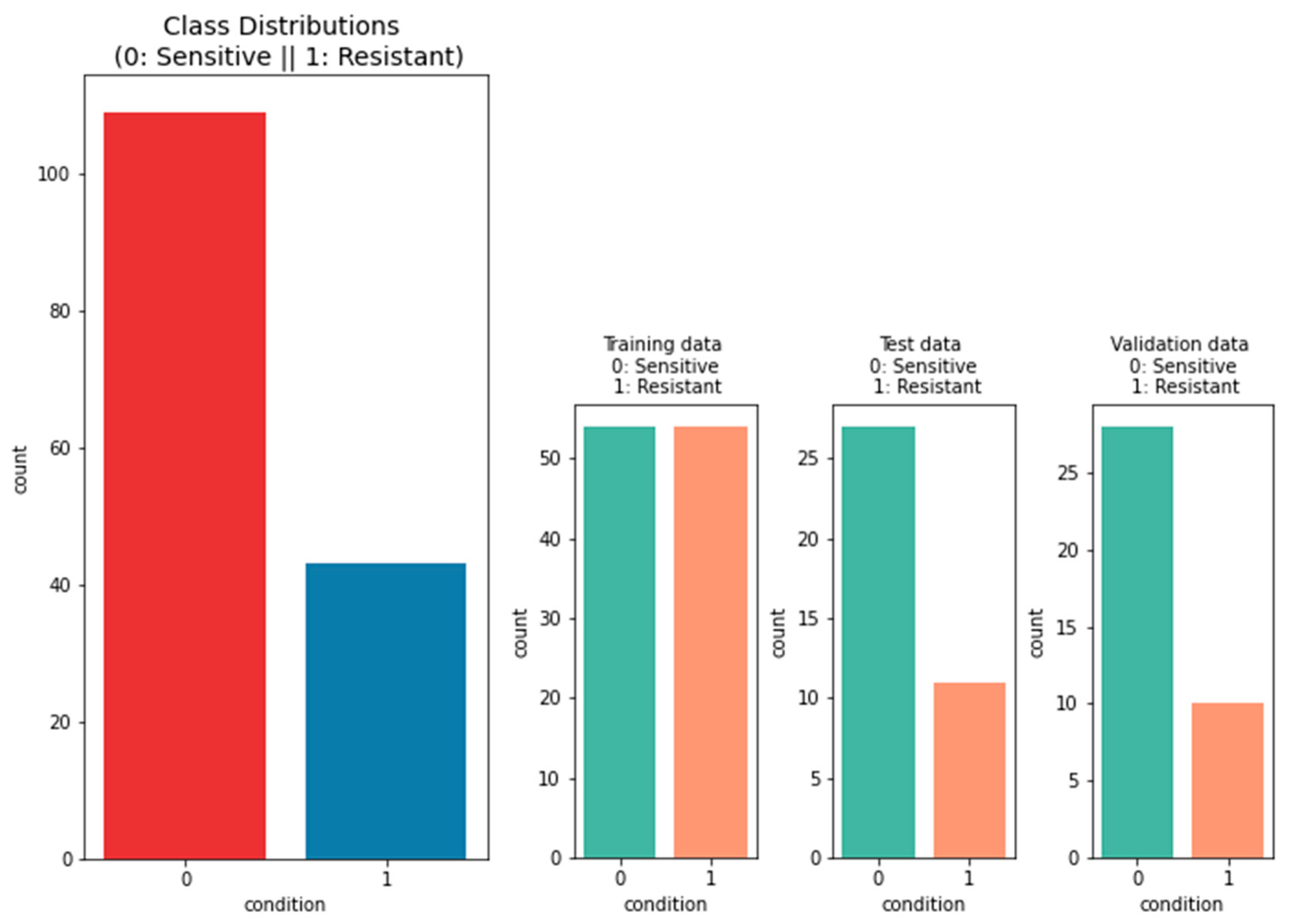
2.1.2. Data on the Platinum Response

To identify genes that could predict platinum response in ovarian cancer, the classification provided by the TCGA study was used. In total, there are 152 patients. And 109 of those are sensitive, and 43 are resistant.

2.2. Methods

2.2.1. Machine Learning Methods
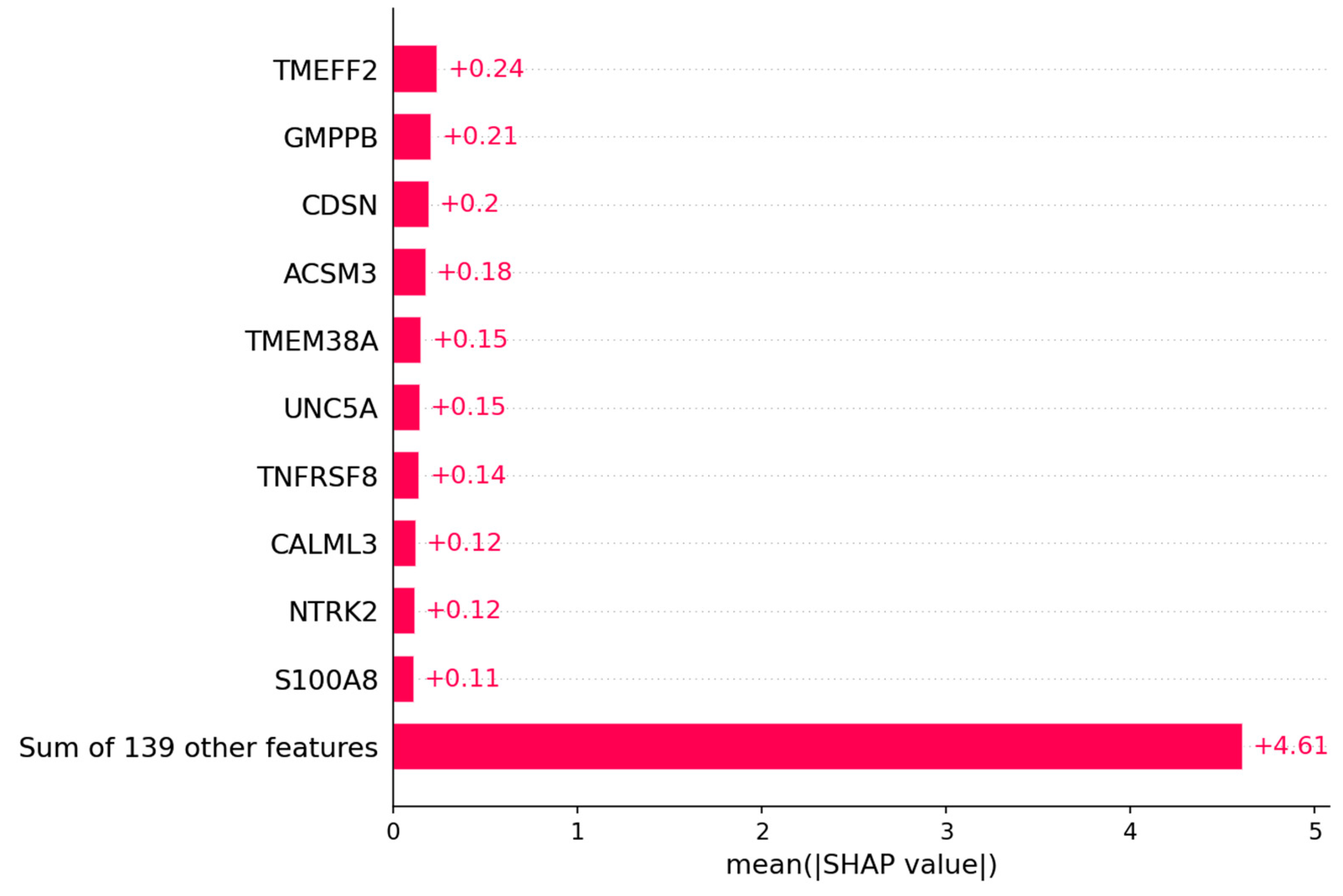
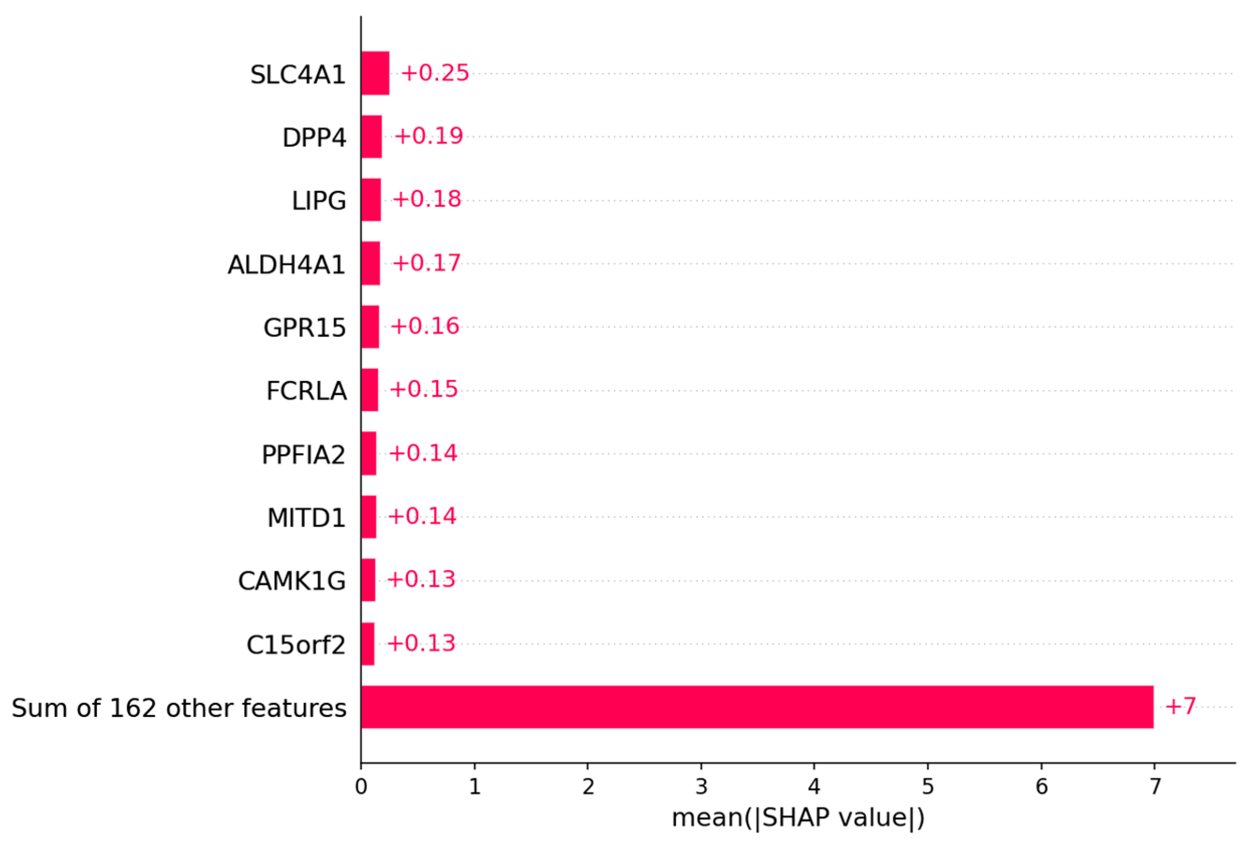
The machine learning methods have been all trained with 50% of the data selected as a training set and then frequently tested on 25% of the data selected as a test set. When the performance reaches the desired value, it is tested once on the remaining 25% to evaluate how well the method performs on unseen data. All of the methods have been trained as binary classifiers to identify the correct class by their gene expression profile. The models have been tested with the normalized data and data from the principal component analysis. The training of the models has been done in different Jupyter Notebooks on the “Cancer Genomics Cloud” provided by Seven Bridges. For each machine learning model, the f1-score, accuracy, sensitivity, and specificity have been calculated to determine their predictive performance. The confusion matrix of the classifiers is used to assess the performance, and scatterplots are used to compare the different metrics across the models. The machine learning methods used in this study are K-means clustering [25,26], Naïve Bayes [27], logistic regression [28,29], supported vector machines [30,31], Random Forest [32,33], and XBGoost [34]. All the methods used were integrated via the sklearn library in Python. For the K-means Clustering method and the Naïve Bayes Classifier, the standard hyperparameters have been used as a reference. For the four other methods, optimization has been achieved using grid search, inputting different hyperparameter sets to find the best-performing model.

2.2.2. SHAP

To determine which genes can be used as biomarkers, the XAI method SHAP is used [20]. All genes add information to the machine learning model that helps predict the outcome or platinum response status of each patient. To estimate which genes contribute the most information, the algorithm utilizes the mathematics from game theory to determine the local and global significance of the genes [35]. The most important metric here is the Shapley value which is described as the difference by including or excluding the gene in a coalition. At first, all Shapley values for each gene are determined by calculating the marginal contribution of each gene to different feature coalitions. The Shapley value for each gene represents the average contribution of a gene across all coalitions. The values are then weighted according to the number of formed coalitions to account for the different combinations of features that can occur. The weighted values are then aggregated to give a comprehensive contribution of each gene to the model’s prediction [20,36].

2.2.3. Bioinformatics Algorithms

The original gene expression data consists of 20,429 genes. Most of them are likely, not relevant in the search for biomarkers because they are not differentially expressed between the two classes. To filter out those genes, we used DESeq2 available in R [23]. In the volcano plot in Figure 3 the significance of the genes is depicted. Figure 3a shows the differentially expressed genes between the patients with good and bad outcome and Figure 3b between the patients that are platinum sensitive or resistant. Unnormalized gene counts are used for that purpose. The counts are normalized using the geometrical mean across all samples for each gene. The gene count is divided by this mean to estimate the size factors using the median of the ratios in each sample. Those accommodate for library size and RNA composition bias. Subsequent steps estimate gene-wise dispersion and shrink estimates to accurate model counts. In the last step, the counts are used to fit a negative binomial model and use the Wald test for hypothesis testing [37]. Afterward, the log2fold shrinkage method apeglm is used to determine which genes have significant changes between the two groups. The p-adjusted value is used to select the genes that are significantly expressed between the two groups. A p-adjusted value of 0.01 is used for the outcome studies and 0.05 for the platinum response studies.
For the outcome studies, genes upregulated in patients with a good outcome have a log2foldchange above zero, and the ones upregulated in patients with a bad outcome have a log2foldchange lower than zero. For the platinum response studies, genes upregulated in platinum-sensitive patients have a log2foldchange above zero, and the ones that are upregulated in platinum-resistant patients have a log2foldchange lower than zero. The selected gene lists are further analyzed to determine their biological implications for ovarian cancer. Metascape has been used for gene set enrichment analysis, pathway analysis, and functional gene annotation. It is a web-based portal to provide those analyses in a combined tool leveraging 40 independent knowledge bases for the assessment [38].

2.2.4. Statistical Methods

After conducting the differential gene expression analysis, the gene count data underwent normalization before utilization in machine-learning algorithms. Considering that the ovarian cancer patient data was generated in batches, it was necessary to normalize the samples both within each gene and across the samples themselves. Two potential normalization methods were considered: the widely used z-normalization and the TMM normalization [39]. The comparative evaluation revealed that the TMM normalization method resulted in improved performance of the machine learning models.
Despite the normalization process, outliers persisted in the data. To address this issue, winsorization was applied. Specifically, the top 2.5% of the mRNA expression values in both groups were replaced with the next highest value. This adjustment was made after observing that these outliers exerted undue influence on the determination of important features, as indicated by feature abstraction using SHAP.
For the platinum response studies, SMOTE [40] was used on the training dataset to balance the sample size of each group. This step was necessary because the initial training dataset is highly imbalanced in favor of the platinum-sensitive group. The machine learning methods do not perform well because the prediction is based more on the frequent class instead of the gene expression values. The SMOTE algorithm draws a random sample from the minority class, and the k-nearest neighbors to that observation are identified. One of them is picked, and the vector between both observations is identified. The vector is multiplied by a number between zero and one and then added to the data point that was originally picked. With this approach, the machine learning models are trained with similar data as the original data points and do not lean to the majority class while the integrity of the data stays intact [40,41]. The distributions of the classes for the patients with good and bad outcome can be seen Figure 4 and for the resistancy status of the patients in Figure 5.
Afterward, all data points for both groups and datasets are scaled between zero and one because some methods, like SVM, perform better with scaling. On the resulting datasets, a PCA is performed since Random Forest and XGBoost classifiers worked better in the approach than without it. This is essentially just for the assessment of the best performer since it is very difficult to transform the principal components later back to the original features [42,43].

3. Results

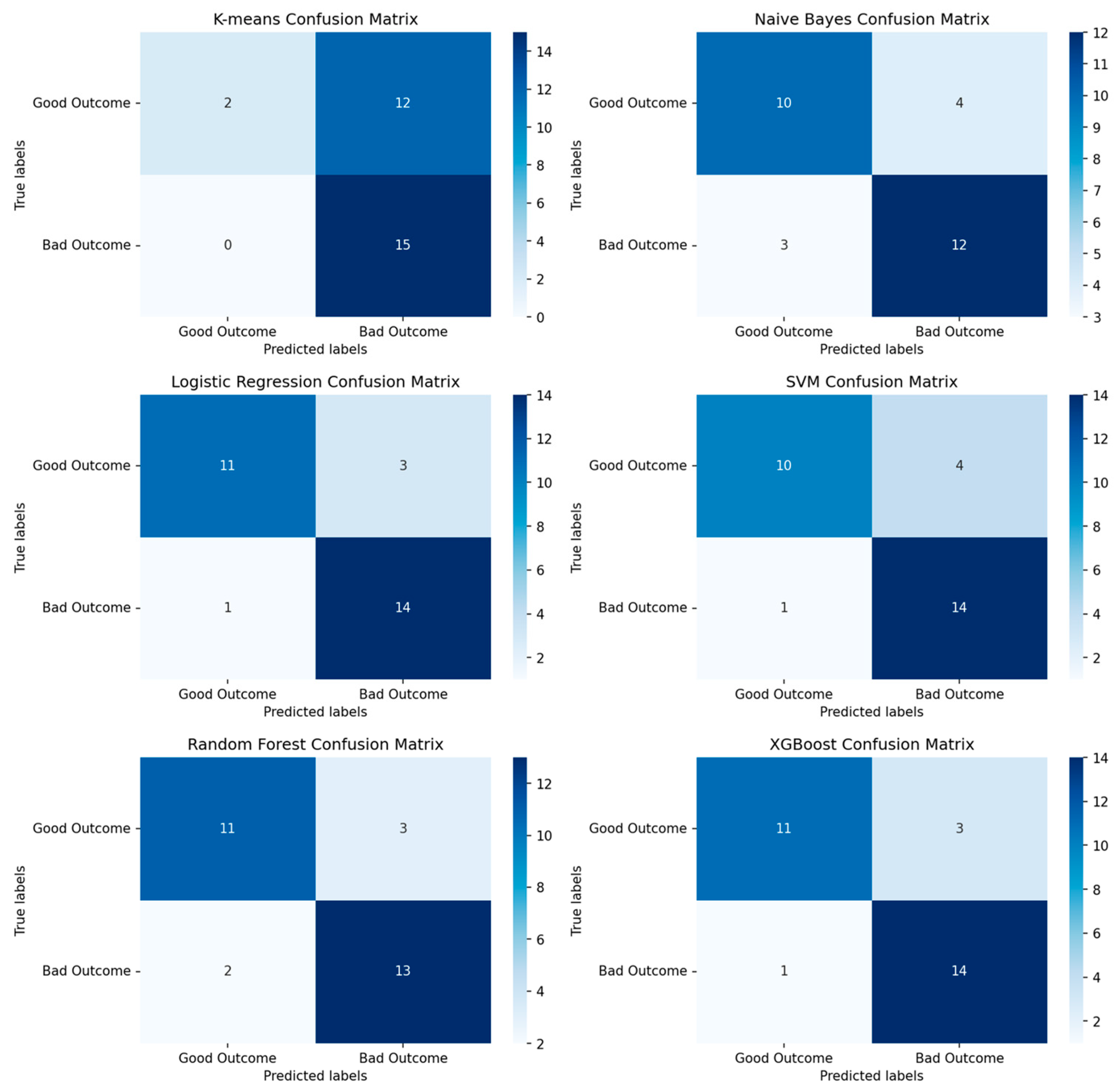
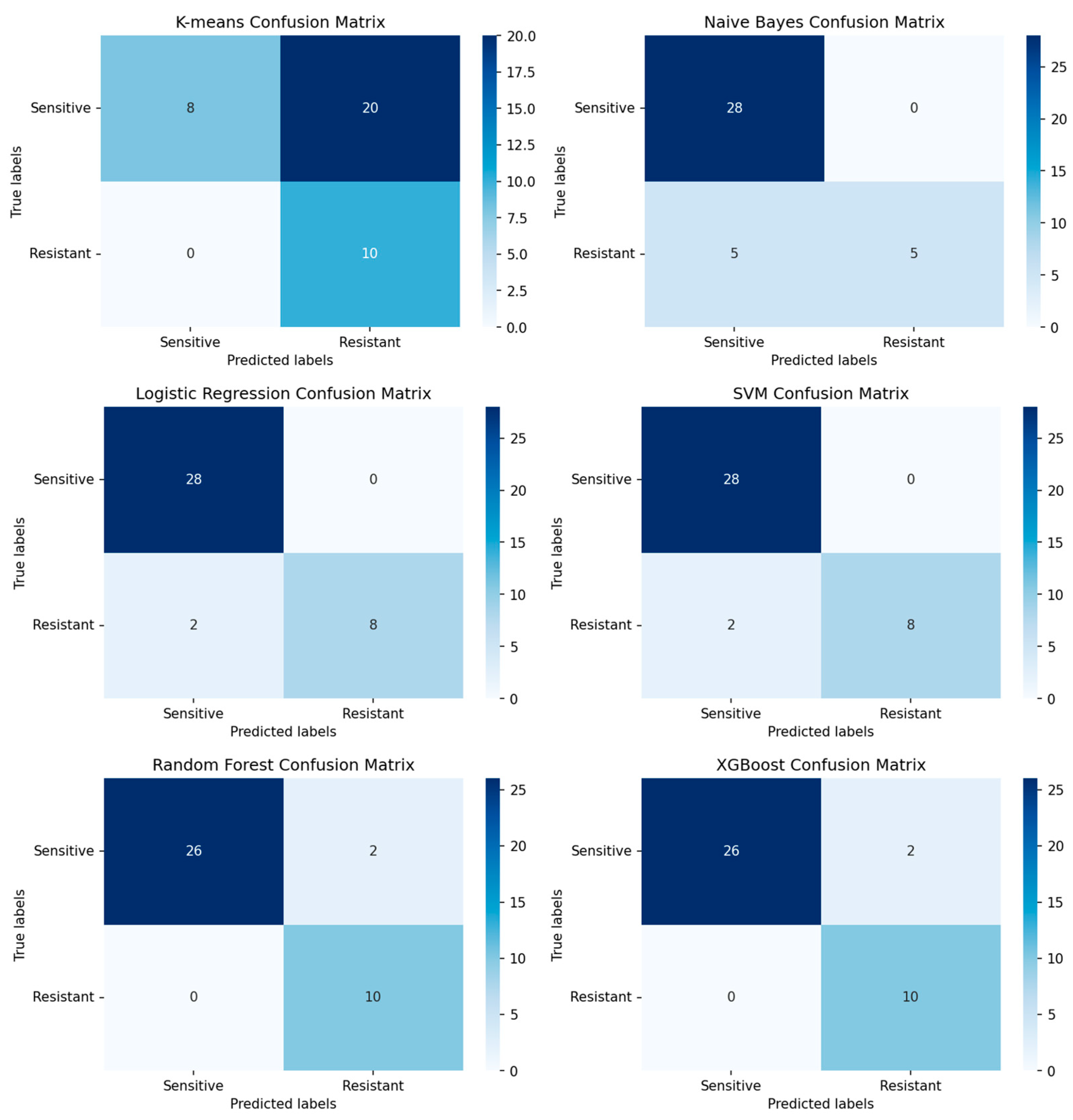
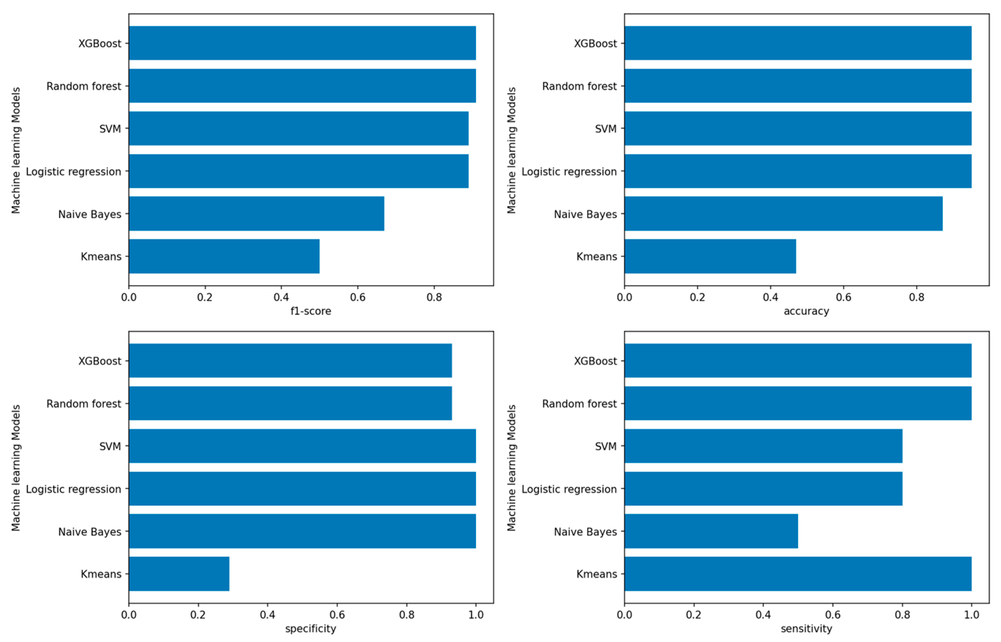
3.1. Performance of Machine-Learning Models

3.1.1. Performance of Machine-Learning Models for Patient Outcome

Six different machine-learning methods were used to predict the outcome of ovarian cancer patients (Figure 6). The performance and accuracy is evaluated by the f1-score, accuracy, specificity and sensitivity of the model on the validation dataset (Figure 7). The best-performing model is the logistic regression model, with 4 misclassifications out of 29 observations. The performance of the other models was slightly lower. The worst-performing model is the K-means-clustering model. For the selection of the genes, the models have been tested on the differentially expressed genes with a p-adjusted value of 0.1, 0.05, and 0.01. The gene dataset with a cutoff of 0.01 consisting of 149 genes was the best-performing one.

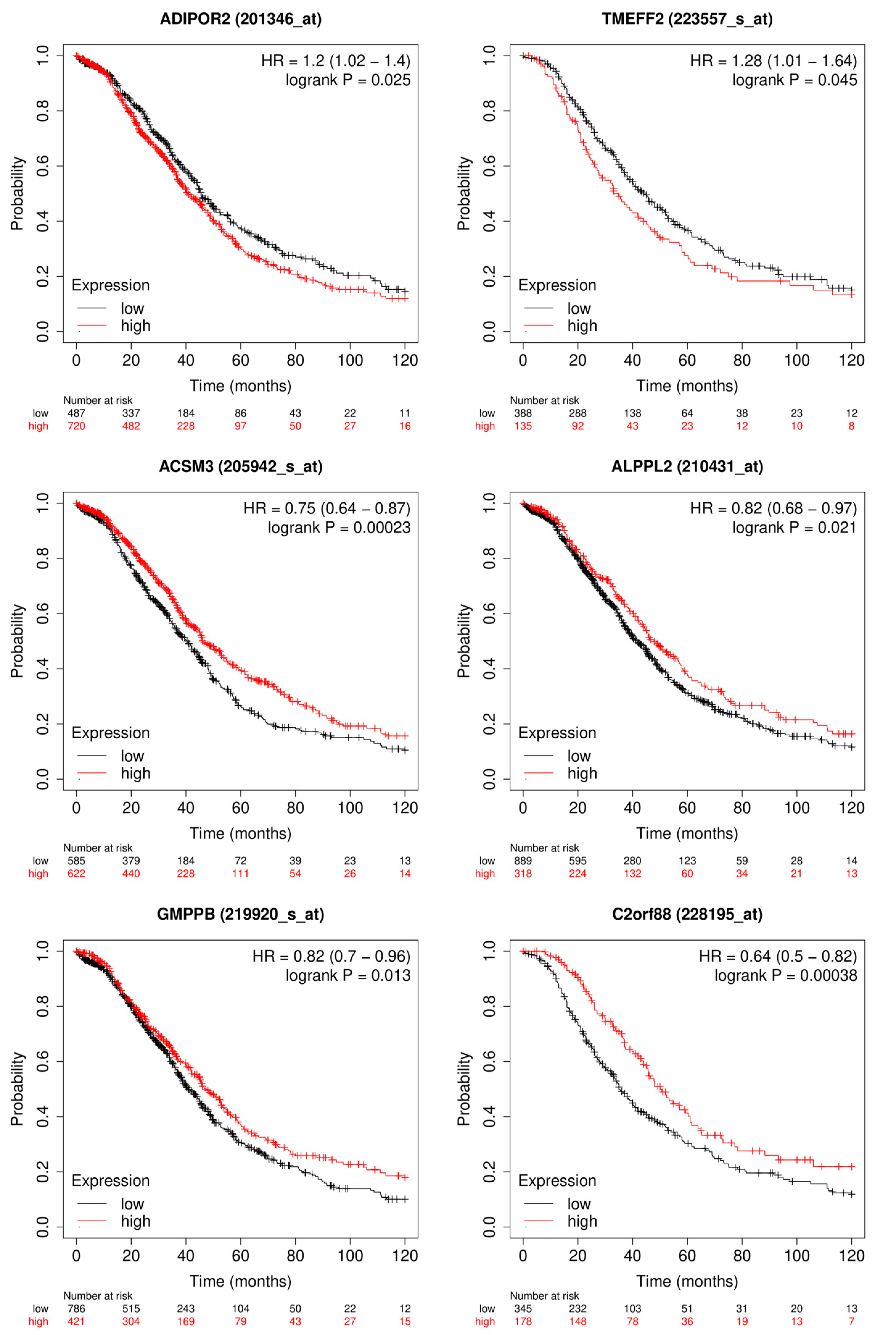
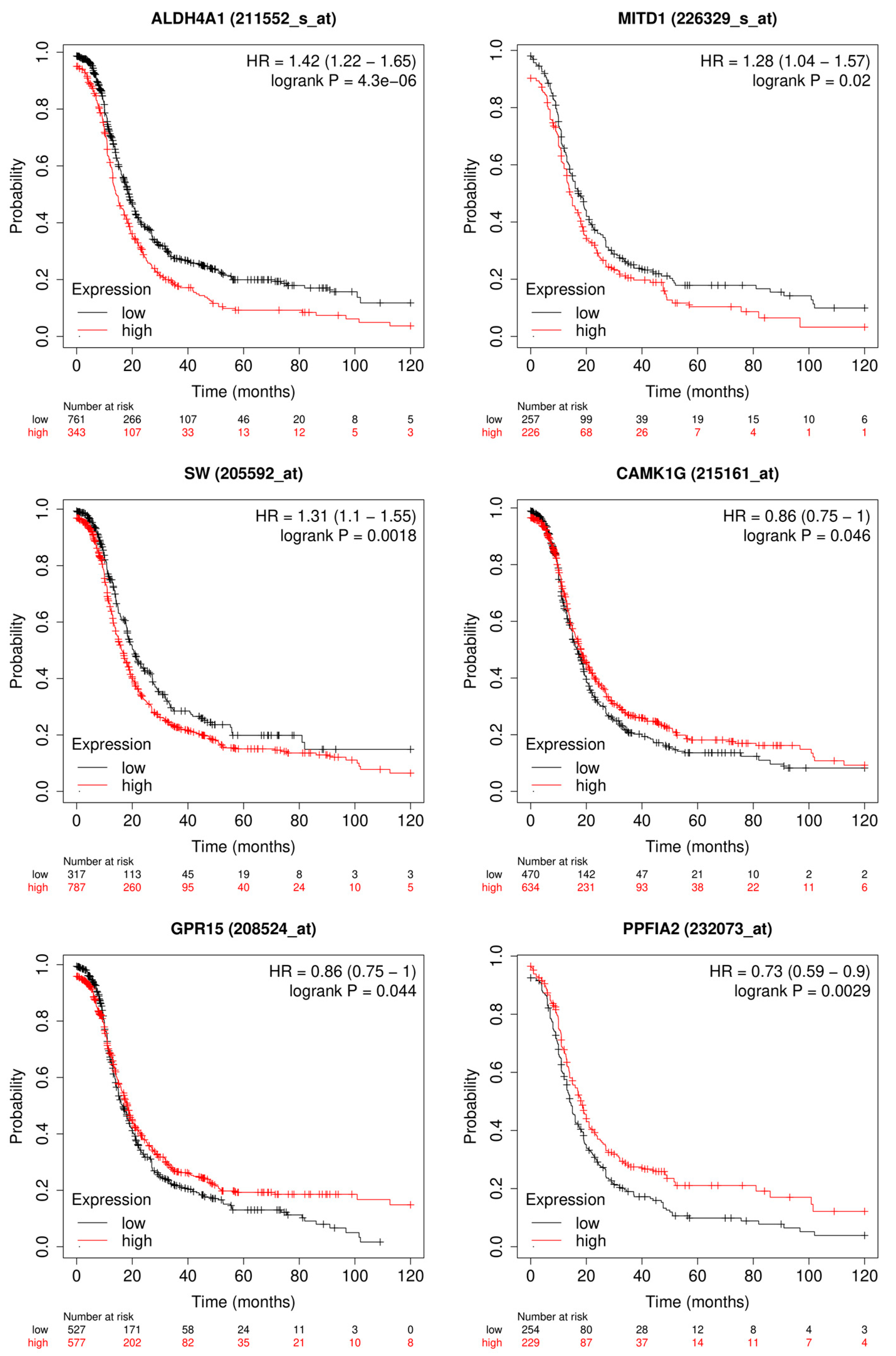
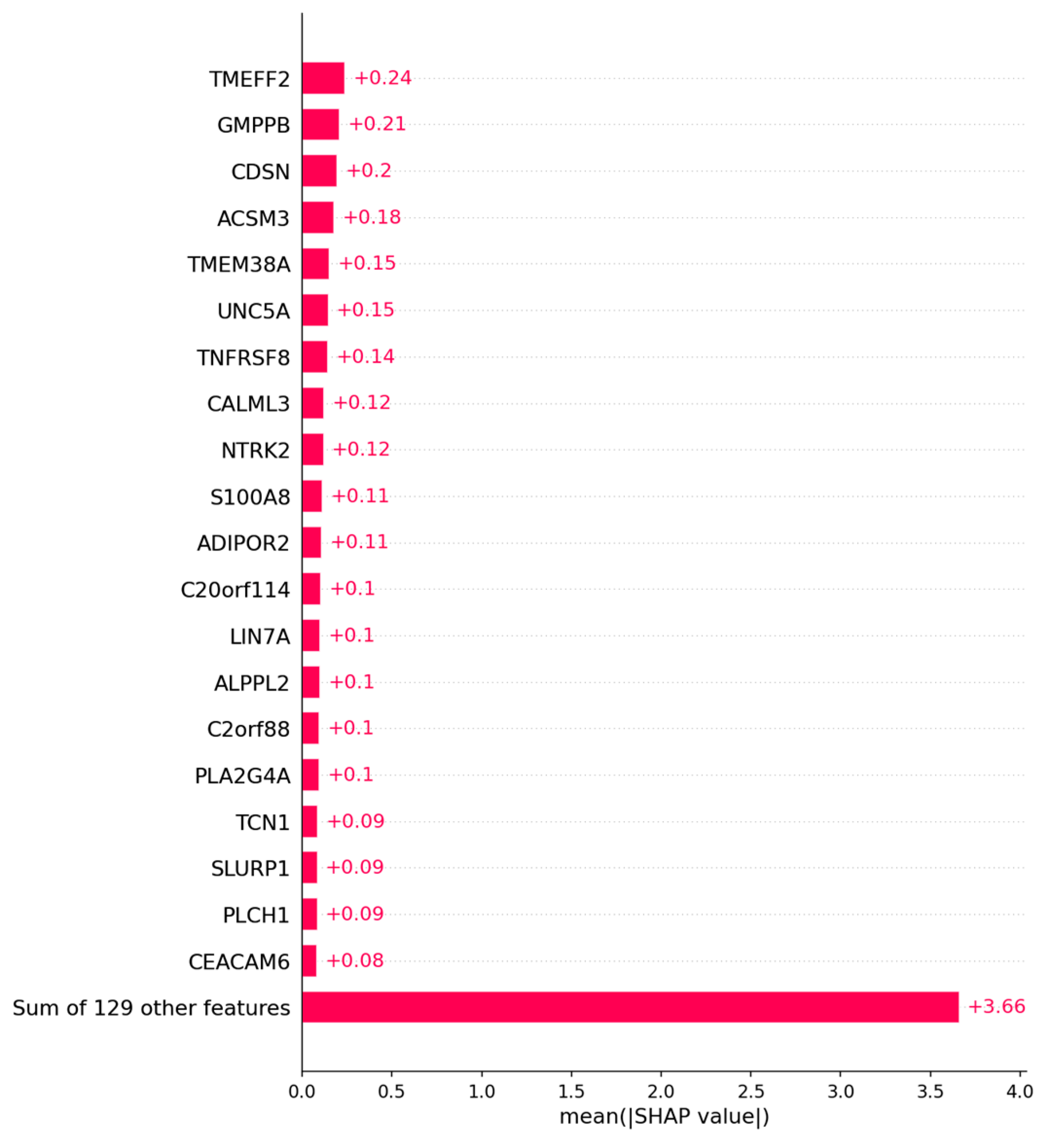
3.1.2. Candidate Genes

The SHAP Algorithm has been performed on the logistic regression model to evaluate which genes have the highest impact on the outcome of the model. The genes with the highest impact on the model are depicted in Figure 8. The top 20 genes with the highest Shapley values can be found in Figure A1. Those genes were then separated into the ones that were upregulated in the good outcome group and those that were upregulated in the bad outcome group. Upregulated in this context means the overall expression of that gene is higher in one group of patients than in the other. In Figure 9, the Kaplan–Meier plots are depicted from six genes with high Shapley values and low adjusted p-values [44]. The first two are upregulated in the group of patients with bad outcomes, and the other four are upregulated in the group of patients with good outcomes.

3.2. Platinum Resistance Prediction of Ovarian Cancer Patients

3.2.1. Performance of Machine-Learning Models for Platinum Response

The same six machine learning methods have been used to predict whether a patient is platinum-sensitive or resistant (Figure 10). The performance and accuracy is evaluated by the f1-score, accuracy, specificity and sensitivity of the model on the validation dataset (Figure 11). The random forest model is the one with the highest f1-score of 0.91 and two misclassifications from 38 observations. The logistic regression model has an f1-score of 0.89 and two misclassifications. The random forest model used the data from the PCA and is, therefore, more difficult to interpret. For the feature analysis with SHAP, the logistic regression model is used instead. The K-means clustering model receives the worst performance score. For the selection of the genes, the models have been tested on the differentially expressed genes with a p-adjusted value of <0.1 and <0.05. The gene dataset with a cutoff of 0.05 consisting of 172 genes was the best-performing one.

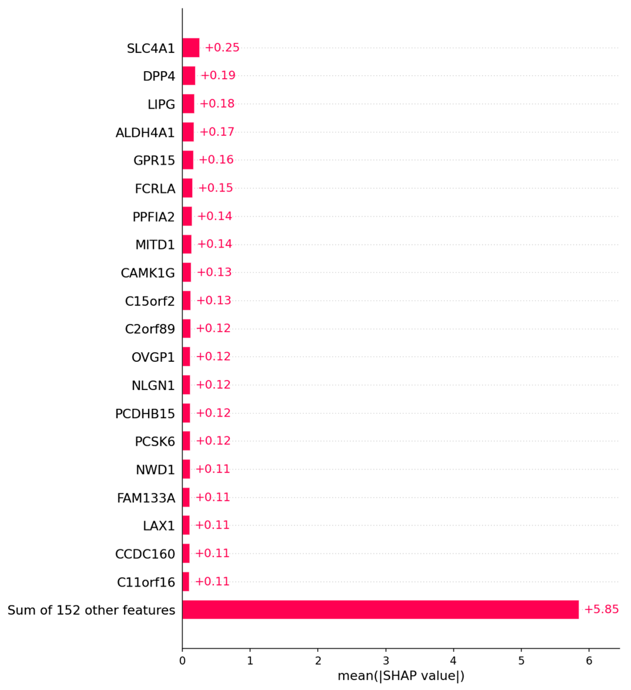
3.2.2. Candidate Genes

For the selection of genes, the SHAP algorithm has been performed on the logistic regression model to evaluate which genes have the highest impact on the prediction of whether the patient is platinum-sensitive or resistant. The genes with the highest impact on the model are depicted in Figure 12. The top 20 genes with the highest Shapley values can be found in Figure A2. Those genes were then separated into the ones that are upregulated in the patient group that is platinum-sensitive and those that are upregulated in the platinum-resistant group. In Figure 13, the Kaplan–Meier plots are depicted from six genes with high Shapley values and low adjusted p-values. The first two are upregulated in the group of patients with bad outcomes, and the other four are upregulated in the group of patients with good outcomes.

4. Discussion

4.1. Outcome Prediction for Patients with Ovarian Cancer

For the outcome prediction based on the gene expression profile, it can be demonstrated that high performance is achieved with common machine learning methods. Apart from the K-means clustering method, all machine learning models had a decent prediction performance. As shown in Figure 6, the models were able to predict good and bad outcomes very well. This is probably due to the data preprocessing steps and filtering of the genes based on their differential expression. With 149 genes from originally 20,429, the data size has decreased significantly, and also, the genes with no or low information value have been removed. Furthermore, the separation of the patients between those that have a very short survival of 2 years or less after their treatment and those with long survival of 5 years or longer probably increased the differences in gene expression as well. In Kaplan–Meier plots (Figure 9), it was possible to identify genes that are significant for the OS of ovarian cancer patients using the SHAP algorithm. TMEFF2 is the gene with the highest median Shapley value. It has been shown that high expression of TMEFF2 in endometrial cancer is correlated with advanced cancer stage, poor differentiation, and lymph node metastasis [45]. Expression is also correlated with the recurrence of the tumor after successful therapy [46]. ADIPOR2 is in the top 20 of the selected genes by SHAP and is correlated, as shown in the Kaplan–Meier plot (Figure 8), with shorter OS survival when highly expressed. It has been shown in chicken ovarian cancer cell lines that ADIPOR2 protein expression is higher in cancerous ovaries than in normal ovaries [47]. ADIPOR2 expression is positively associated with proliferation and lethality in prostate cancer [48]. ACSM3 is number four of the median Shapley values. High expression of this gene, on the other hand, is correlated with inhibited cell proliferation, migration, and invasion of ovarian cancer cells. Overexpression of the gene even led to suppression in cell migration [49]. Moreover, in high-grade serous ovarian carcinoma (HGSOC), ACSM3 can suppress tumor growth in vitro and in vivo [50]. Even though the biological implications of ALPPL2 remains unclear, high expression of the gene is correlated with good outcome in patients, as shown in Figure 8, and it has been reported as a true tumor-specific antigen [51]. For GMPPB, the increased expression is correlated with favorable outcomes. There is little information about its role in cancer, but two studies identified the gene as a predictive marker in ovarian cancer as well [52,53]. The last gene shown is C2orf88 which is upregulated in patients with longer OS. Regarding the biological function C2orf88, it is only predicted that it enables protein kinase A regulatory subunit binding activity [54]. But it is a prognostic factor for ovarian cancer patients.
Furthermore, the pathway and annotation analysis in Appendix B Table A1 shows TNFRSF8 and TIGAR in multiple pathways. For the pathway analysis, genes with a SHAP value up to 0.01 have been considered. The highly expressed genes from the bad outcome group have been used in the analysis. The TNFRSF8 and TIGAR are associated with pathways for positive regulation of the apoptotic process and programmed cell death, which is interesting since both were shown in studies to be associated with bad outcomes in patients. TNFRSF8 upregulation has been linked to several downregulated genes in pathways for cell death, cell-mediated immune response, and inflammatory response [55]. It has also been exploited as a therapeutic target using monoclonal antibody monotherapy [56]. For TIGAR, it has been shown that its higher expression is associated with poor overall survival in ovarian cancer as well as the knockdown of the gene enhances sensitivity to the PARP inhibitors in cancer cells [57]. PARP Inhibitors are used to treat advanced BRCA-mutated ovarian cancer in adults [58]. The results of the pathway analysis of the upregulated genes in patients with good outcomes did not show any significant results.
The two most promising genes to function as a biomarker and as a prognostic factor are TMEFF2 and ACSM3 due to their high significance and known biological functions.

4.2. Prediction of Platinum Response Status

It was possible to create multiple well-performing machine-learning models to predict whether a patient is platinum-sensitive or resistant. The highest score reached the random forest model with an f1-score of 0.91. The principal components from the PCA have been used as input. In the studies reported by Nasimian et al. [21], they used a similar approach and trained a deep learning model with a much bigger patient cohort with 2616 samples. The best performance of their model in predicting the platinum resistance status of patients had an f1-score of 83.1. The higher performance of the random forest model used here could be due to the different data preprocessing or the smaller sample size [21]. In Figure 13 the Kaplan–Meier plots of three genes that are upregulated in patients with platinum sensitivity and three genes that are upregulated in patients with resistance are depicted. In comparison to the outcome prediction, the plots in Figure 13 show the PFS of ovarian cancer patients instead. The reason for it is that patients that have a recurrence within 6 months after treatment are considered resistant, and patients that have no recurrences or one after 6 months are considered sensitive. Therefore, the PFS is a better fit to identify genes that are associated with platinum response. SLC4A1 (SW) has the highest median Shapley value, and its increased expression is correlated with low PFS. The gene is upregulated in patients that are resistant to platinum. As stated in another paper, the gene is an independent prognostic factor for poor OS in grade 3 or 4 serous ovarian cancer [59]. The protein AE1 is a chloride/bicarbonate transporter that is encoded by SLC4A1. AEs are important in regulating intracellular pH [60]. Alterations in pH are frequently altered in different types of cancer, like ovarian cancer [61,62]. ALDH4A1 has the fourth-highest median Shapley value, and its high expression of it is highly correlated with platinum resistance and poor PFS. The gene has been associated by other studies with chemoresistance and might mediate carboplatin resistance [63,64]. MITD1 is the last one of the platinum-resistant group, and the high expression of this gene is associated with low PFS [65]. The protein coded by MITD1 is recruited by ESCRT-III to midbodies and participates afterward in cytokinesis abscission [66]. Alterations in MITD1 expression may affect ESCRT-III function in cytokinesis abscission, aneuploidy, and response to platinum. High expression of CAMK1G is associated with longer PFS survival, and it is upregulated in patients that are platinum sensitive. The gene belongs to the protein kinase I family, and these enzymes control a wide range of functions in cancer and might be potential therapeutic targets [67]. GPR15 has the same prognostic attribution as CAMK1G. GPR15 expression is higher in normal tissue than in tumors in colon and lung adenocarcinomas and has the potential, with its natural ligand, to inhibit cancer cell growth [68]. High gene expression of PPFIA2 is highly correlated with longer PFS in ovarian cancer patients. Not too much research has been performed to identify the correlation between PPFIA2 and cancer types but the protein it encodes binds to calcium/calmodulin-dependent kinases [69]. It has already been suggested that Ca2+ signaling is important in cancer cell function so there might be a correlation between Ca2+ pathways and acquiring platinum resistance.
The pathway analysis for the higher expressed genes in the resistant patients showed enhancement of cell–cell adhesion and cell–cell adhesion via plasma–membrane adhesion molecules, as can be seen in Appendix B Table A2. The p-value < 0.01 cutoff has resulted in 20 genes upregulated in the resistant patients. The two genes in the named pathways are NLGN1 and PCDHB15. Studies show that NLGN1 is highly expressed in clusters of aggressive migrating single tumor cells and promotes trans-endothelial migration [70]. For PCDHB15, a similar aggressive behavior was identified. It has been shown that overexpression in melanoma leads to invasiveness and aggregation of metastatic melanoma in vitro and forming lung metastasis in vivo [71]. Taken together, we suggest that both genes alter the biological process of cell–cell adhesion and the process of plasma membrane adhesion molecules [72]. Multiple papers show that cell–cell adhesion and adhesion molecules play a vital role in cancer. Many cell adhesion molecules act as tumor suppressors and, when altered, can promote the proliferation and migration of cancer cells [73,74,75]. Potentially, the increased migration leads to higher chemotherapy resistance since the therapy targets cells with high proliferation, and according to the “go” or “grow” hypothesis, proliferation and migration spatiotemporally exclude one another [76]. Further experimental investigation is needed to prove that hypothesis.

5. Conclusions

It has been demonstrated in this approach that it is possible to predict the outcome and resistance status of ovarian cancer patients and identify biologically relevant genes. The most promising potential biomarkers are TMEFF2, ACSM3, SLC4A1, and ALDH4A1. Their SHAP median values were high; they had a strong correlation with OS or PFS, and their biological functions affect cancer. In addition to that, the pathway analysis, in combination with the SHAP median values, suggests that NLGN1, PCDHB15, TIGAR, and TNFRSF8 are potential biomarkers of ovarian cancer.

Author Contributions

Conceptualization, V.S., P.B. and J.C.; data curation, V.S.; formal analysis, V.S.; funding acquisition, J.C.; investigation, V.S. and J.C.; methodology, V.S., P.B. and J.C.; project administration, J.C.; resources, J.C.; software, V.S. and J.C.; supervision, P.B. and J.C.; validation, V.S. and J.C.; visualization, V.S.; writing—original draft, V.S.; writing—review and editing, V.S., P.B. and J.C. All authors have read and agreed to the published version of the manuscript..

Funding

This research received no external funding.

Data Availability Statement

For the analysis, the publicly available ovarian cancer data by the TCGA has been used. For further questions on how to obtain the data, please contact the authors.

Acknowledgments

We acknowledge Alice Barr for providing gynecological/oncological expertise.

Conflicts of Interest

The authors declare no conflict of interest, financial or otherwise.

Appendix A

Figure A1. The bar plot shows the top 20 genes based on the mean SHAP value of the logistic regression model of the ovarian cancer outcome prediction.
Algorithms 16 00330 g0a1
Figure A2. The bar plot shows the top 20 genes based on the mean SHAP value of the logistic regression model of the platinum resistance prediction.
Algorithms 16 00330 g0a2

Appendix B

Table A1. Pathway enrichment analysis of the upregulated genes in the patients having bad outcomes with SHAP values of 0.01 or higher.
CategoryGODescriptionHits
GO Biological ProcessesGO:0042886amide transportNTRK2|S100A8|SLC1A6
Immunologic SignaturesM5353GSE37416 0H vs. 48H F TULARENSIS LVS NEUTROPHIL DNTNFRSF8|CATSPERG|ADIPOR2
GO Biological ProcessesGO:0042060wound healingS100A8|TMEFF2|ADIPOR2
GO Biological ProcessesGO:0099537trans-synaptic signalingNTRK2|SLC1A6|LIN7A
GO Biological ProcessesGO:0048514blood vessel morphogenesisNTRK2|ANGPTL4|ADIPOR2
GO Biological ProcessesGO:0009611response to woundingS100A8|TMEFF2|ADIPOR2
GO Biological ProcessesGO:0099536synaptic signalingNTRK2|SLC1A6|LIN7A
GO Biological ProcessesGO:0001568blood vessel developmentNTRK2|ANGPTL4|ADIPOR2
GO Biological ProcessesGO:0046903secretionNTRK2|S100A8|LIN7A
GO Biological ProcessesGO:0001944vasculature developmentNTRK2|ANGPTL4|ADIPOR2
GO Biological ProcessesGO:0043065positive regulation of apoptotic processTNFRSF8|S100A8|TIGAR
GO Biological ProcessesGO:0043068positive regulation of programmed cell deathTNFRSF8|S100A8|TIGAR
GO Biological ProcessesGO:0010942positive regulation of cell deathTNFRSF8|S100A8|TIGAR
GO Biological ProcessesGO:0030855epithelial cell differentiationCDSN|CASP14|TIGAR
GO Biological ProcessesGO:0035239tube morphogenesisNTRK2|ANGPTL4|ADIPOR2
Reactome Gene SetsR-HSA-382551Transport of small moleculesAPOC4|SLC1A6|ANGPTL4
Table A2. Pathway enrichment analysis of the upregulated genes in the patients that are platinum-resistant with SHAP value of 0.01 or higher.
CategoryGODescriptionHits
GO Biological ProcessesGO:0098742cell–cell adhesion via plasma–membrane adhesion moleculesNLGN1|PCDHB15|
PCDHB7
GO Biological ProcessesGO:0098609cell–cell adhesionNLGN1|PCDHB15|
PCDHB7

References

  1. Ovarian Cancer Survival Rates|Ovarian Cancer Prognosis. Available online: https://www.cancer.org/cancer/ovarian-cancer/detection-diagnosis-staging/survival-rates.html (accessed on 28 March 2023).
  2. Surgery for Recurrent Ovarian Cancer May Help Selected Patients-NCI. Available online: https://www.cancer.gov/news-events/cancer-currents-blog/2022/ovarian-cancer-return-surgery-desktop-iii (accessed on 28 March 2023).
  3. Flynn, M.J.; Ledermann, J.A. Ovarian Cancer Recurrence: Is the Definition of Platinum Resistance Modified by PARPi and Other Intervening Treatments? The Evolving Landscape in the Management of Platinum-Resistant Ovarian Cancer. Cancer Drug Resist. 2022, 5, 424–435. [Google Scholar] [CrossRef] [PubMed]
  4. Jayson, G.C.; Kohn, E.C.; Kitchener, H.C.; Ledermann, J.A. Ovarian Cancer. Lancet 2014, 384, 1376–1388. [Google Scholar] [CrossRef] [PubMed]
  5. How to Check for Ovarian Cancer|Ovarian Cancer Screening. Available online: https://www.cancer.org/cancer/ovarian-cancer/detection-diagnosis-staging/detection.html (accessed on 26 April 2023).
  6. Klein, M.E.; Dabbs, D.J.; Shuai, Y.; Brufsky, A.M.; Jankowitz, R.; Puhalla, S.L.; Bhargava, R. Prediction of the Oncotype DX Recurrence Score: Use of Pathology-Generated Equations Derived by Linear Regression Analysis. Mod. Pathol. 2013, 26, 658–664. [Google Scholar] [CrossRef] [Green Version]
  7. Kumar, L.; Greiner, R. Gene Expression Based Survival Prediction for Cancer Patients—A Topic Modeling Approach. PLoS ONE 2019, 14, e0224446. [Google Scholar] [CrossRef] [PubMed]
  8. Cardoso, F.; van’t Veer, L.J.; Bogaerts, J.; Slaets, L.; Viale, G.; Delaloge, S.; Pierga, J.-Y.; Brain, E.; Causeret, S.; DeLorenzi, M.; et al. 70-Gene Signature as an Aid to Treatment Decisions in Early-Stage Breast Cancer. N. Engl. J. Med. 2016, 375, 717–729. [Google Scholar] [CrossRef] [Green Version]
  9. Tang, Z.; Li, C.; Kang, B.; Gao, G.; Li, C.; Zhang, Z. GEPIA: A Web Server for Cancer and Normal Gene Expression Profiling and Interactive Analyses. Nucleic Acids Res. 2017, 45, W98–W102. [Google Scholar] [CrossRef] [Green Version]
  10. Ghoniem, R.M.; Algarni, A.D.; Refky, B.; Ewees, A.A. Multi-Modal Evolutionary Deep Learning Model for Ovarian Cancer Diagnosis. Symmetry 2021, 13, 643. [Google Scholar] [CrossRef]
  11. Hartmann, L.C.; Lu, K.H.; Linette, G.P.; Cliby, W.A.; Kalli, K.R.; Gershenson, D.; Bast, R.C.; Stec, J.; Iartchouk, N.; Smith, D.I.; et al. Gene Expression Profiles Predict Early Relapse in Ovarian Cancer after Platinum-Paclitaxel Chemotherapy. Clin. Cancer Res. 2005, 11, 2149–2155. [Google Scholar] [CrossRef] [Green Version]
  12. Millstein, J.; Budden, T.; Goode, E.L.; Anglesio, M.S.; Talhouk, A.; Intermaggio, M.P.; Leong, H.S.; Chen, S.; Elatre, W.; Gilks, B.; et al. Prognostic Gene Expression Signature for High-Grade Serous Ovarian Cancer. Ann. Oncol. 2020, 31, 1240–1250. [Google Scholar] [CrossRef]
  13. Konstantinopoulos, P.A.; Spentzos, D.; Cannistra, S.A. Gene-Expression Profiling in Epithelial Ovarian Cancer. Nat. Rev. Clin. Oncol. 2008, 5, 577–587. [Google Scholar] [CrossRef]
  14. Welsh, J.B.; Zarrinkar, P.P.; Sapinoso, L.M.; Kern, S.G.; Behling, C.A.; Monk, B.J.; Lockhart, D.J.; Burger, R.A.; Hampton, G.M. Analysis of Gene Expression Profiles in Normal and Neoplastic Ovarian Tissue Samples Identifies Candidate Molecular Markers of Epithelial Ovarian Cancer. Proc. Natl. Acad. Sci. USA 2001, 98, 1176–1181. [Google Scholar] [CrossRef]
  15. Spentzos, D.; Levine, D.A.; Ramoni, M.F.; Joseph, M.; Gu, X.; Boyd, J.; Libermann, T.A.; Cannistra, S.A. Gene Expression Signature with Independent Prognostic Significance in Epithelial Ovarian Cancer. J. Clin. Oncol. 2004, 22, 4700–4710. [Google Scholar] [CrossRef] [PubMed]
  16. Yang, N.; Kaur, S.; Volinia, S.; Greshock, J.; Lassus, H.; Hasegawa, K.; Liang, S.; Leminen, A.; Deng, S.; Smith, L.; et al. MicroRNA Microarray Identifies Let-7i as a Novel Biomarker and Therapeutic Target in Human Epithelial Ovarian Cancer. Cancer Res. 2008, 68, 10307–10314. [Google Scholar] [CrossRef] [PubMed] [Green Version]
  17. Bell, D.; Berchuck, A.; Birrer, M.; Chien, J.; Cramer, D.W.; Dao, F.; Dhir, R.; DiSaia, P.; Gabra, H.; Glenn, P.; et al. Integrated Genomic Analyses of Ovarian Carcinoma. Nature 2011, 474, 609–615. [Google Scholar] [CrossRef] [Green Version]
  18. Verhaak, R.G.W.; Tamayo, P.; Yang, J.-Y.; Hubbard, D.; Zhang, H.; Creighton, C.J.; Fereday, S.; Lawrence, M.; Carter, S.L.; Mermel, C.H.; et al. Prognostically Relevant Gene Signatures of High-Grade Serous Ovarian Carcinoma. J. Clin. Investig. 2013, 123, 517–525. [Google Scholar] [CrossRef] [PubMed]
  19. Zhang, W.; Ota, T.; Shridhar, V.; Chien, J.; Wu, B.; Kuang, R. Network-Based Survival Analysis Reveals Subnetwork Signatures for Predicting Outcomes of Ovarian Cancer Treatment. PLoS Comput. Biol. 2013, 9, e1002975. [Google Scholar] [CrossRef] [Green Version]
  20. Lundberg, S.; Lee, S.-I. A Unified Approach to Interpreting Model Predictions. arXiv 2017. [Google Scholar] [CrossRef]
  21. Nasimian, A.; Ahmed, M.; Hedenfalk, I.; Kazi, J.U. A Deep Tabular Data Learning Model Predicting Cisplatin Sensitivity Identifies BCL2L1 Dependency in Cancer. Comput. Struct. Biotechnol. J. 2023, 21, 956–964. [Google Scholar] [CrossRef]
  22. Weinstein, J.N.; Collisson, E.A.; Mills, G.B.; Shaw, K.R.M.; Ozenberger, B.A.; Ellrott, K.; Shmulevich, I.; Sander, C.; Stuart, J.M. The Cancer Genome Atlas Pan-Cancer Analysis Project. Nat. Genet. 2013, 45, 1113–1120. [Google Scholar] [CrossRef]
  23. Love, M.I.; Huber, W.; Anders, S. Moderated Estimation of Fold Change and Dispersion for RNA-Seq Data with DESeq2. Genome Biol. 2014, 15, 550. [Google Scholar] [CrossRef] [Green Version]
  24. CBioPortal for Cancer Genomics. Available online: https://www.cbioportal.org/study/clinicalData?id=ov_tcga_pan_can_atlas_2018 (accessed on 4 June 2023).
  25. Steinhaus, H. Bulletin de L’Académie Polonaise Des Sciences: Série des sciences mathématiques, astronomiques, et physiques. Państowowe Wydawn 1956, 4, 801–804. [Google Scholar]
  26. Lloyd, S. Least Squares Quantization in PCM. IEEE Trans. Inform. Theory 1982, 28, 129–137. [Google Scholar] [CrossRef] [Green Version]
  27. Bayes, T.; Price, R. LII. An Essay towards Solving a Problem in the Doctrine of Chances. By the Late Rev. Mr. Bayes, F. R. S. Communicated by Mr. Price, in a Letter to John Canton, A. M. F. R. S. Philos. Trans. R. Soc. Lond. 1763, 53, 370–418. [Google Scholar] [CrossRef] [Green Version]
  28. Garnier, J.-G.; Quetelet, A. Correspondance Mathématique et Physique; Hayez, M., Imprimeur; Harvard University: Cambridge, MA, USA, 1838; Volume 10. [Google Scholar]
  29. Verhulst, P.-F. Recherches Mathématiques sur la loi D’accroissement de la Population; Nouveaux Mémoires de l’Académie Royale des Sciences et Belles-Lettres de Bruxelles, Harvard University: Cambridge, MA, USA, 1845; pp. 14–54. [Google Scholar]
  30. Vapnik, V.N.; Lerner, A.Y. Recognition of Patterns with help of Generalized Portraits. Recognit. Patterns Help. Gen. Portraits 1963, 24, 774–780. [Google Scholar]
  31. Cortes, C.; Vapnik, V. Support-Vector Networks. Mach. Learn. 1995, 20, 273–297. [Google Scholar] [CrossRef]
  32. Ho, T.K. Random Decision Forests. In Proceedings of the 3rd International Conference on Document Analysis and Recognition, Montreal, QC, Canada, 14–16 August 1995; Volume 1, pp. 278–282. [Google Scholar] [CrossRef]
  33. Breiman, L. Random Forests. Mach. Learn. 2001, 45, 5–32. [Google Scholar] [CrossRef] [Green Version]
  34. Chen, T.; Guestrin, C. XGBoost: A Scalable Tree Boosting System. In Proceedings of the 22nd ACM SIGKDD International Conference on Knowledge Discovery and Data Mining, San Francisco, CA, USA, 13 August 2016; pp. 785–794. [Google Scholar]
  35. Shapley, L.S. Stochastic Games*. Proc. Natl. Acad. Sci. USA 1953, 39, 1095–1100. [Google Scholar] [CrossRef]
  36. Kuo, C. Explain Your Model with the SHAP Values. Medium. 2019. Available online: https://medium.com/dataman-in-ai/explain-your-model-with-the-shap-values-bc36aac4de3d (accessed on 31 May 2023).
  37. Piper, M.M.; Khetani, R.; Gene-Level, M. Differential Expression Analysis with DESeq2. Available online: https://hbctraining.github.io/DGE_workshop/lessons/04_DGE_DESeq2_analysis.html (accessed on 31 May 2023).
  38. Zhou, Y.; Zhou, B.; Pache, L.; Chang, M.; Khodabakhshi, A.H.; Tanaseichuk, O.; Benner, C.; Chanda, S.K. Metascape Provides a Biologist-Oriented Resource for the Analysis of Systems-Level Datasets. Nat. Commun. 2019, 10, 1523. [Google Scholar] [CrossRef] [Green Version]
  39. Robinson, M.D.; Oshlack, A. A Scaling Normalization Method for Differential Expression Analysis of RNA-Seq Data. Genome Biol. 2010, 11, R25. [Google Scholar] [CrossRef] [Green Version]
  40. Chawla, N.V.; Bowyer, K.W.; Hall, L.O.; Kegelmeyer, W.P. SMOTE: Synthetic Minority over-Sampling Technique. J. Artif. Int. Res. 2002, 16, 321–357. [Google Scholar] [CrossRef]
  41. Korstanje, J. SMOTE. Available online: https://towardsdatascience.com/smote-fdce2f605729 (accessed on 31 May 2023).
  42. Pearson, K. LIII. On Lines and Planes of Closest Fit to Systems of Points in Space. Lond. Edinb. Dublin Philos. Mag. J. Sci. 1901, 2, 559–572. [Google Scholar] [CrossRef] [Green Version]
  43. Hotelling, H. Analysis of a Complex of Statistical Variables into Principal Components. J. Educ. Psychol. 1933, 24, 417–441. [Google Scholar] [CrossRef]
  44. Kaplan, E.L.; Meier, P. Nonparametric Estimation from Incomplete Observations. J. Am. Stat. Assoc. 1958, 53, 457–481. [Google Scholar] [CrossRef]
  45. Gao, L.; Nie, X.; Zheng, M.; Li, X.; Guo, Q.; Liu, J.; Liu, Q.; Hao, Y.; Lin, B. TMEFF2 Is a Novel Prognosis Signature and Target for Endometrial Carcinoma. Life Sci. 2020, 243, 116910. [Google Scholar] [CrossRef]
  46. Alabiad, M.A.; Harb, O.A.; Hefzi, N.; Ahmed, R.Z.; Osman, G.; Shalaby, A.M.; Alnemr, A.A.-A.; Saraya, Y.S. Prognostic and Clinicopathological Significance of TMEFF2, SMOC-2, and SOX17 Expression in Endometrial Carcinoma. Exp. Mol. Pathol. 2021, 122, 104670. [Google Scholar] [CrossRef] [PubMed]
  47. Tiwari, A.; Ocon-Grove, O.M.; Hadley, J.A.; Giles, J.R.; Johnson, P.A.; Ramachandran, R. Expression of Adiponectin and Its Receptors Is Altered in Epithelial Ovarian Tumors and Ascites-Derived Ovarian Cancer Cell Lines. Int. J. Gynecol. Cancer 2015, 25. [Google Scholar] [CrossRef] [PubMed]
  48. Rider, J.R.; Fiorentino, M.; Kelly, R.; Gerke, T.; Jordahl, K.; Sinnott, J.A.; Giovannucci, E.L.; Loda, M.; Mucci, L.A.; Finn, S. Tumor Expression of Adiponectin Receptor 2 and Lethal Prostate Cancer. Carcinogenesis 2015, 36, 639–647. [Google Scholar] [CrossRef] [Green Version]
  49. Yan, L.; He, Z.; Li, W.; Liu, N.; Gao, S. The Overexpression of Acyl-CoA Medium-Chain Synthetase-3 (ACSM3) Suppresses the Ovarian Cancer Progression via the Inhibition of Integrin Β1/AKT Signaling Pathway. Front. Oncol. 2021, 11, 644840. [Google Scholar] [CrossRef]
  50. Yang, X.; Wu, G.; Zhang, Q.; Chen, X.; Li, J.; Han, Q.; Yang, L.; Wang, C.; Huang, M.; Li, Y.; et al. ACSM3 Suppresses the Pathogenesis of High-Grade Serous Ovarian Carcinoma via Promoting AMPK Activity. Cell Oncol. 2022, 45, 151–161. [Google Scholar] [CrossRef]
  51. Su, Y.; Zhang, X.; Bidlingmaier, S.; Behrens, C.R.; Lee, N.-K.; Liu, B. ALPPL2 Is a Highly Specific and Targetable Tumor Cell Surface Antigen. Cancer Res. 2020, 80, 4552–4564. [Google Scholar] [CrossRef]
  52. Liu, J.; Li, S.; Feng, G.; Meng, H.; Nie, S.; Sun, R.; Yang, J.; Cheng, W. Nine Glycolysis-Related Gene Signature Predicting the Survival of Patients with Endometrial Adenocarcinoma. Cancer Cell Int. 2020, 20, 183. [Google Scholar] [CrossRef]
  53. Bi, J.; Bi, F.; Pan, X.; Yang, Q. Establishment of a Novel Glycolysis-Related Prognostic Gene Signature for Ovarian Cancer and Its Relationships with Immune Infiltration of the Tumor Microenvironment. J. Transl. Med. 2021, 19, 382. [Google Scholar] [CrossRef] [PubMed]
  54. C2orf88 Chromosome 2 Open Reading Frame 88 [Homo Sapiens (Human)]-Gene-NCBI. Available online: https://www.ncbi.nlm.nih.gov/gene/84281#summary (accessed on 26 April 2023).
  55. Vallacchi, V.; Vergani, E.; Camisaschi, C.; Deho, P.; Cabras, A.D.; Sensi, M.; De Cecco, L.; Bassani, N.; Ambrogi, F.; Carbone, A.; et al. Transcriptional Profiling of Melanoma Sentinel Nodes Identify Patients with Poor Outcome and Reveal an Association of CD30+ T Lymphocytes with Progression. Cancer Res. 2014, 74, 130–140. [Google Scholar] [CrossRef] [PubMed] [Green Version]
  56. van der Weyden, C.A.; Pileri, S.A.; Feldman, A.L.; Whisstock, J.; Prince, H.M. Understanding CD30 Biology and Therapeutic Targeting: A Historical Perspective Providing Insight into Future Directions. Blood Cancer J. 2017, 7, e603. [Google Scholar] [CrossRef] [PubMed] [Green Version]
  57. Fang, P.; De Souza, C.; Minn, K.; Chien, J. Genome-Scale CRISPR Knockout Screen Identifies TIGAR as a Modifier of PARP Inhibitor Sensitivity. Commun. Biol. 2019, 2, 335. [Google Scholar] [CrossRef] [Green Version]
  58. Bixel, K.; Hays, J.L. Olaparib in the Management of Ovarian Cancer. Pharmgenomics Pers. Med. 2015, 8, 127–135. [Google Scholar] [CrossRef] [Green Version]
  59. Qin, L.; Li, T.; Liu, Y. High SLC4A11 Expression Is an Independent Predictor for Poor Overall Survival in Grade 3/4 Serous Ovarian Cancer. PLoS ONE 2017, 12, e0187385. [Google Scholar] [CrossRef] [Green Version]
  60. Zhang, L.-J.; Lu, R.; Song, Y.-N.; Zhu, J.-Y.; Xia, W.; Zhang, M.; Shao, Z.-Y.; Huang, Y.; Zhou, Y.; Zhang, H.; et al. Knockdown of Anion Exchanger 2 Suppressed the Growth of Ovarian Cancer Cells via MTOR/P70S6K1 Signaling. Sci. Rep. 2017, 7, 6362. [Google Scholar] [CrossRef] [Green Version]
  61. Parks, S.K.; Chiche, J.; Pouysségur, J. Disrupting Proton Dynamics and Energy Metabolism for Cancer Therapy. Nat. Rev. Cancer 2013, 13, 611–623. [Google Scholar] [CrossRef]
  62. Damaghi, M.; Wojtkowiak, J.; Gillies, R. PH Sensing and Regulation in Cancer. Front. Physiol. 2013, 4, 370. [Google Scholar] [CrossRef] [Green Version]
  63. Tomita, H.; Tanaka, K.; Tanaka, T.; Hara, A. Aldehyde Dehydrogenase 1A1 in Stem Cells and Cancer. Oncotarget 2016, 7, 11018. [Google Scholar] [CrossRef] [PubMed] [Green Version]
  64. Ginestier, C.; Korkaya, H.; Dontu, G.; Birnbaum, D.; Wicha, M.S.; Charafe-Jauffret, E. The cancer stem cell: The breast cancer driver. Med. Sci. 2007, 23, 1133–1139. [Google Scholar] [CrossRef] [Green Version]
  65. Dong, S.; Hou, D.; Peng, Y.; Chen, X.; Li, H.; Wang, H. Pan-Cancer Analysis of the Prognostic and Immunotherapeutic Value of MITD1. Cells 2022, 11, 3308. [Google Scholar] [CrossRef] [PubMed]
  66. Lee, S.; Chang, J.; Renvoisé, B.; Tipirneni, A.; Yang, S.; Blackstone, C. MITD1 Is Recruited to Midbodies by ESCRT-III and Participates in Cytokinesis. Mol. Biol. Cell 2012, 23, 4347–4361. [Google Scholar] [CrossRef] [PubMed]
  67. Brzozowski, J.S.; Skelding, K.A. The Multi-Functional Calcium/Calmodulin Stimulated Protein Kinase (CaMK) Family: Emerging Targets for Anti-Cancer Therapeutic Intervention. Pharmaceuticals 2019, 12, 8. [Google Scholar] [CrossRef] [Green Version]
  68. Wang, Y.; Wang, X.; Xiong, Y.; Li, C.-D.; Xu, Q.; Shen, L.; Chandra Kaushik, A.; Wei, D.-Q. An Integrated Pan-Cancer Analysis and Structure-Based Virtual Screening of GPR15. Int. J. Mol. Sci. 2019, 20, 6226. [Google Scholar] [CrossRef] [Green Version]
  69. PPFIA2 PTPRF Interacting Protein Alpha 2 [Homo Sapiens (Human)]-Gene-NCBI. Available online: https://www.ncbi.nlm.nih.gov/gene/8499#summary (accessed on 27 April 2023).
  70. Pergolizzi, M.; Bizzozero, L.; Maione, F.; Maldi, E.; Isella, C.; Macagno, M.; Mariella, E.; Bardelli, A.; Medico, E.; Marchiò, C.; et al. The Neuronal Protein Neuroligin 1 Promotes Colorectal Cancer Progression by Modulating the APC/β-Catenin Pathway. J. Exp. Clin. Cancer Res. 2022, 41, 266. [Google Scholar] [CrossRef]
  71. Carrier, A.; Desjobert, C.; Lobjois, V.; Rigal, L.; Busato, F.; Tost, J.; Ensenyat-Mendez, M.; Marzese, D.M.; Pradines, A.; Favre, G.; et al. Epigenetically Regulated PCDHB15 Impairs Aggressiveness of Metastatic Melanoma Cells. Clin. Epigenetics 2022, 14, 156. [Google Scholar] [CrossRef]
  72. Ashburner, M.; Ball, C.A.; Blake, J.A.; Botstein, D.; Butler, H.; Cherry, J.M.; Davis, A.P.; Dolinski, K.; Dwight, S.S.; Eppig, J.T.; et al. Gene Ontology: Tool for the Unification of Biology. Nat. Genet. 2000, 25, 25–29. [Google Scholar] [CrossRef] [Green Version]
  73. Janiszewska, M.; Primi, M.C.; Izard, T. Cell Adhesion in Cancer: Beyond the Migration of Single Cells. J. Biol. Chem. 2020, 295, 2495–2505. [Google Scholar] [CrossRef] [Green Version]
  74. Moh, M.C.; Shen, S. The Roles of Cell Adhesion Molecules in Tumor Suppression and Cell Migration: A New Paradox. Cell Adh Migr. 2009, 3, 334–336. [Google Scholar] [CrossRef] [PubMed] [Green Version]
  75. Hartmann, T.N. Editorial: Metabolism and Cell Adhesion in Cancer. Front. Cell Dev. Biol. 2022, 10, 871471. [Google Scholar] [CrossRef] [PubMed]
  76. Garay, T.; Juhász, É.; Molnár, E.; Eisenbauer, M.; Czirók, A.; Dekan, B.; László, V.; Hoda, M.A.; Döme, B.; Tímár, J.; et al. Cell Migration or Cytokinesis and Proliferation? – Revisiting the “Go or Grow” Hypothesis in Cancer Cells in Vitro. Exp. Cell Res. 2013, 319, 3094–3103. [Google Scholar] [CrossRef] [PubMed]
Figure 1. The schematic shows the overall project structure. The study consists of 585 patients, but biological and clinical data from some patients are not available, and they are excluded. Patients are put into two very distinct categories: for example, good or bad outcome groups or resistant or sensitive groups. After the group classification, patients are distributed into three datasets: 50% training data, 25% testing data, and 25% validation data to avoid overfitting the data. The performance of the models is determined with a one-time test on the validation data set. Patients and their features are used as the input for the machine learning models to predict the class of each patient. When the performance of the models is sufficient, algorithms from the field of explainable artificial intelligence will be applied to detect which biological features contribute the most to the decision of the model. Those features likely have the most biological impact on patient outcomes.
Algorithms 16 00330 g001
Figure 2. The patients are separated into three groups. The first group consists of patients with shorter OS and consists of 113 patients. They died within the first two years after treatment and are considered to have a bad outcome. The second group consists of patients with longer OS and consists of 119 patients. They have lived five years and longer after treatment and are considered to have a good outcome. The third group consists of all patients in between the two groups and makes up the biggest portion with 345. Those patients were excluded from the initial studies. The thresholds were chosen to have two groups that were very distinct from one another to make changes and differences in their gene expression profile easier to detect.
Algorithms 16 00330 g002
Figure 3. (a) The volcano plot shows the differentially expressed genes between the patients with good or bad outcomes. The dots in green represent genes that have an adjusted p-value of <0.01 and a log2FoldChange between +2 and −2. The red dots represent genes that have an adjusted p-value of <0.01 and a log2FoldChange >2 or <−2. The blue dots are all genes that have an adjusted p-value of >0.01. (b) The volcano plot depicted shows the differentially expressed genes between the patients that are sensitive or resistant to platinum-based chemotherapy. The dots in green represent genes that have an adjusted p-value of <0.05 and a log2FoldChange between +2 and −2. The red dots represent genes that have an adjusted p-value of <0.05 and a log2FoldChang >2 or <−2. The blue dots are all genes that have an adjusted p-value > 0.05.
Algorithms 16 00330 g003aAlgorithms 16 00330 g003b
Figure 4. The left bar plot depicts the overall data distribution of samples used for the outcome studies. Fifty-five patients are considered to have a good outcome, and 57 patients are considered to have a bad outcome. The distribution between the two classes is balanced, so there is no need for over- or under-sampling. In the bar plots on the right, the distribution of the classes is shown between the training data, test data, and validation data.
Algorithms 16 00330 g004
Figure 5. The left bar plot depicts the overall data distribution for platinum response studies. A total of 109 patients are considered to be sensitive, and 43 patients are considered to be resistant. The distribution between the two classes is unbalanced. Oversampling is used to adjust that in the training data. In the bar plots on the right, the distribution of the classes is shown between the training data, test data, and validation data.
Algorithms 16 00330 g005
Figure 6. Confusion matrices for the different machine learning methods. The higher the number for the concordance between true labels and predicted labels, the more accurate and trustworthy the model is. F1-scores that evaluate the performance of the model are K-means Clustering: 0.71, Naïve Bayes: 0.77, Logistic Regression: 0.88, Supported Vector Machine: 0.85, Random Forest: 0.84, XGBoost: 0.88. The logistic regression- and the XGBoost model receive the highest f1-scores with 4 misclassifications from 29 observations. For higher interpretability, the logistic regression model is used for further analysis.
Algorithms 16 00330 g006
Figure 7. Barplots highlight the metrics: f1-score, accuracy, sensitivity, and specificity for the models predicting the good or bad outcomes of ovarian cancer patients. The model with the highest overall metrics is the Logistic Regression model. Apart from the f1-score, the XGBoost model matches those metrics in all other categories. The worst-performing model is the K-means clustering method in terms of the assessed four metrics.
Algorithms 16 00330 g007
Figure 8. The bar plot shows the top 10 genes based on the mean SHAP value of the logistic regression model of the ovarian cancer outcome prediction.
Algorithms 16 00330 g008
Figure 9. Kaplan–Meier plots for OS of the most relevant genes for the logistic regression model. ADIPOR2 and TMEFF2 are upregulated in the group of patients with bad outcomes. ACSM3, ALPPL2, GMPPB, and C2orf88 are upregulated in the group of patients with a good outcome.
Algorithms 16 00330 g009
Figure 10. Confusion matrices for the different machine learning methods used in this study. The higher the number of concordances between true labels and predicted labels, the more accurate and trustworthy the model is. The f1-scores for the models are K-means Clustering: 0.5, Naïve Bayes: 0.67, Logistic Regression: 0.89, Supported Vector Machine: 0.89, Random Forest: 0.91, XGBoost: 0.91. The random forest and XGBoost models are the ones with the highest f1-score and two misclassifications from 38 observations. For higher interpretability, the logistic regression model is used for further analysis with a similar f1-score.
Algorithms 16 00330 g010
Figure 11. Barplots highlight the metrics: f1-score, accuracy, sensitivity, and specificity for the models predicting the platinum sensitivity of ovarian cancer patients. The model with the highest overall metrics is the Logistic Regression model. Apart from the f1-score, the XGBoost model matches those metrics in all other categories. The worst-performing model is the K-means clustering method in terms of the assessed four metrics.
Algorithms 16 00330 g011
Figure 12. The bar plot shows the top 10 genes based on the mean SHAP value of the logistic regression model of the platinum resistance prediction.
Algorithms 16 00330 g012
Figure 13. Kaplan–Meier plots for progression-free survival (PFS) of the most relevant genes for the logistic regression model. The genes: ALDH4A1, MITD1, and SLC4A1 (SW) are upregulated in patients with platinum resistance. The genes: CAMK1G, GPR15, and PPFIA2 are upregulated in the patients that are platinum sensitive.
Algorithms 16 00330 g013
Disclaimer/Publisher’s Note: The statements, opinions and data contained in all publications are solely those of the individual author(s) and contributor(s) and not of MDPI and/or the editor(s). MDPI and/or the editor(s) disclaim responsibility for any injury to people or property resulting from any ideas, methods, instructions or products referred to in the content.

