Attention–Survival Score: A Metric to Choose Better Keywords and Improve Visibility of Information

Abstract

In this paper, we propose a method to aid authors in choosing alternative keywords that help their papers gain visibility. These alternative keywords must have a certain level of popularity in the scientific community and, simultaneously, be keywords with fewer competitors. The competitors are derived from other papers containing the same keywords. Having fewer competitors would allow an author’s paper to have a higher consult frequency. In order to recommend keywords, we must first determine an attention–survival score. The attention score is obtained using the popularity of a keyword. The survival score is derived from the number of manuscripts using the same keyword. With these two scores, we created a new algorithm that finds alternative keywords with a high attention–survival score. We used ontologies to ensure that alternative keywords proposed by our method are semantically related to the original authors’ keywords that they wish to refine. The hierarchical structure in an ontology supports the relationship between the alternative and input keywords. To test the sensibility of the ontology, we used two sources: WordNet and the Computer Science Ontology (CSO). Finally, we launched a survey for the human validation of our algorithm using keywords from Web of Science papers and three ontologies: WordNet, CSO, and DBpedia. We obtained good results from all our tests.

1. Introduction

Authors use keywords to emphasize the most important topics of their papers. Keywords can play an important role when other researchers use recommendation systems to discover works related to a specified set of input terms. In addition, journals provide keywords with the title and abstract as part of the preliminary public information about a paper, so this information can be crucial for a researcher to determine whether they will read the full paper. Nevertheless, keyword selection is a process that is not perfect and often has many problems, such as selecting very specific or very generic keywords, misprints, author bias, and inexperience. These biases are aggravated by choosing keywords without following a keyword selection methodology.

When choosing generic or trendy terms, authors face the risk of sharing these terms with many papers that will compete with each other to claim researchers’ attention. However, in choosing rare or specific terms, there is the risk of using terms that do not attract researchers.

In this paper, we studied how popularity relates to higher competition among keywords when choosing them for a manuscript. We analyzed ontologies and, by doing so, we were able to intuitively understand whether generic terms tend to be more popular, as well as more crowded, than specific ones. We aimed to formalize properties that would help us study this phenomenon, and we continued by analyzing the structure of keywords using an ontology.

While in the field of information retrieval we can find different measures to extract topics and keywords, such as TF-IDF, in this paper, we focused on the effects of social behaviors on the keywords and how different tendencies can affect the visibility of the information.

Finally, after the analytic stage, we propose a method to help authors refine their keyword selection processes. This method is based on measuring the popularity and crowding of desired terms while using the knowledge provided by ontologies to enhance the keywords proposed by an author.

This paper is structured as follows:

• Section 1 provides a literature review, which describes the current state-of-the-art theory that underpins the paper;
• Section 2 details the attention–survival model, which presents our theoretical proposal;
• Section 3 provides information on our experimental design, including details about the dataset used, an analysis of the WordNet and CSO ontologies, and examples illustrating our refinement algorithm;
• Section 4 summarizes our conclusions based on the results obtained from our experimental design;

Finally, this work contains a Supplementary Information Section with more information regarding the algorithm results as well as the first and the second experiments.

2. Literature Review

The International Organization for Standardization defines keywords as a word or group of words, possibly in a lexicographically standardized form, taken out of a title or the text of a document characterizing its content and enabling its retrieval [1]. Apart from texts, keywords are often used to describe the content of a work by using words that contain the essential topics or themes that are represented in the work. For example, papers in the scientific community frequently come with a set of keywords, typically six. When authors decide what keywords they want to use for their manuscripts, we call them author keywords. The author can choose these keywords freely or from a prespecified list of terms [2]. Sometimes, keywords are extracted using automatic procedures. This is the case for KeyWords Plus, where keywords are selected from the titles of articles cited in the references section [3].

Keywords can have multiple applications, with one of the most used being information retrieval, where the scientific community uses keywords to search for information on certain topics [4,5,6]. Keywords are also used to easily identify the most relevant content of an article, study the behavior of authors [7,8], map the structure of the science [9], or build a taxonomy, among others [10]. In order to detect research trends [11], author-defined keywords are used to represent topics in an ex ante approach, called author-defined keyword frequency prediction (AKFP), to detect research trends. Another example is searching by keywords using a traditional web service [12].

Nowadays, plenty of search engines enable researchers to discover papers by typing in a set of keywords. Search engine users prefer this approach because users do not worry about grammatical rules; hence, they require less time and effort to formulate a query [13]. Then the search engine presents a list of recommended papers related to keywords, and the researcher can choose from them. This process was analyzed by [14], who proposed a method to refine this recommendation process by choosing popular articles and very correlated keywords.

Aside from articles, keywords also have different degrees of popularity [15]. Keyword popularity is a topic that has gained attention in the field of marketing research. [16] studied the different behaviors among customers who searched for popular terms and customers who used less popular keywords, concluding that the second group of customers spent more effort on their search process and were more likely to buy something in the end.

It is also relevant to note that author keywords can prevent interpretation biases by other authors [8]. Nevertheless, author keywords are not free from other types of biases, as there are differences between experienced and nonexperienced authors [6].

Authors’ behavior when choosing keywords was studied by [5]. This paper performed a study on the habits of authors and editors regarding keywords, finding that, in the case of authors, it was very common to simply select as many keywords as desired, while editors tended to let authors choose the keywords for a manuscript. Hartley and Kostoff (2003) also focused on the problems generated by the inability of some authors to choose good keywords and the inefficiency of search systems. Some of the problems mentioned are the use of ambiguous keywords and the overuse of keywords without justification.

For authors, it is crucial to select the correct keywords so that their papers are more easily visible to others. At the same time, from an editor’s point of view, having a manuscript with proper keywords can help them improve their journal’s impact [17].

Some strategies have been proposed to mitigate the effects of selecting poor keywords. For example, [2] grouped terms with a similar meaning into single primary terms, while [9], in addition to removing excessively specific words, divided generic terms into specific ones. Intuitively, it seems that using overly generic or overly specific keywords is bad practice.

In the computer science field, ontologies are an explicit specification of a conceptualization [18]. Ontologies represent concepts and their relations in terms of generalization and specificity and can have different applications in fields such as artificial intelligence, web semantics, or linguistics [19,20].

Ontologies have multiple applications in information retrieval and keywords. For example, [21] used ontologies to process natural language. The input words were expanded into related concepts that help to create a keyword domain. [22] built a dynamic ontology based on the Computer Science Ontology. With the help of Word2Vec, the ontology was expanded in order to identify new academic research areas. [23] proposed a paradigm to provide webpage recommendations using semantic information and semantic ontologies. Their paradigm uses the similarity between words and a keyword expansion mechanism to identify new terms that may be interesting for the user who performs a search.

In addition, ontologies have been used to obtain the topics of documents. For example, [24,25] used an ontology structure to determine the topic of a web document. In [26] study, the semantic similarity among academic documents was determined. For this, the authors calculated the similarity between topic events based on the domain ontology to acquire the semantic similarity between articles.

3. The Attention–Survival Model

3.1. Basic Model

Our theoretical model is based on the premise that there is an information retrieval system in which the user introduces a set of keywords. The system randomly returns a list of papers that contain all these keywords but in a random order, and from there, the user chooses one of the returned articles. We consider that the paper the user selects is the only one that “survives” the process.

Our basic model does not consider different biases that would typically exist in an information retrieval system, such as ordering by citation, relevance, impact factor, and publication date, as well as the attention bias generated by the user when choosing an article.

An example of a more complex model where the information retrieval system is biased with respect to the publication date is presented in the Appendix A.

3.2. The Attention–Survival Score

Let $K_j=\left\{k_1,k_2,\dots ,k_n\right\}$ be the set of initial candidate keywords, as defined by the user for manuscript $j$.

When authors search for manuscripts by entering specific inputs, we presume that only one manuscript will be extracted from each search process. Therefore, we denote the article selected as the survivor manuscript.

Let $C\left(k\right)$ be the community of keyword $k$. We define community as the set of manuscripts that contains a given keyword. $C\left(k\right)$ defines the set of articles containing the keyword $k;$ thus, they are the ones that will compete with our manuscripts to survive.

Let $S\left(k\right),k\in K$ be the survival score of a keyword. Given an article that contains the keyword $k$, $S\left(k\right)$ is the propensity of the keyword to survive, according to our basic model. We assume that our recommendation system is neutral so that the retrieval process is unbiased. In order to help readers understand our model, we did not consider values by relevance, length, cites, impact, or publication date (i.e., basic model). If we apply a biased retrieval process, then we have to redefine $S\left(k\right),k\in K$ according to the bias applied. This situation is explained in Appendix A. Under our basic model supposition, the survival score is defined as follows:

$$S\left(k\right)=\frac{1}{\left|C\left(k\right)\right|}$$

We consider that an author can look for either one keyword (e.g., $k$) or a set of them (e.g., $K$). When looking for multiple keywords at the same time, the community $C\left(K\right)$ is described as the set of manuscripts that contains every keyword in $K$ simultaneously.

We can compute the survival score of $K$ as follows:

$$S_{\cup }\left(K\right)=\frac{\sum S\left(k_i\right)}{\left|K\right|}$$

where $K=\left\{k_1,k_2,\dots ,k_n\right\}$.

Another important concept in our work is keyword attention, $A\left(k\right)$, which is the level of interest shown by the community for a certain keyword. As discussed later in the paper, the attention of a word is a function of the number of times that word is used in a query. We derived this value using information provided by Google Trends.

Similarly, we can compute the attention of a set of keywords as the average value of the attention scores from every keyword in the input set. This is presented as

$$A_{\cup }\left(K\right)=\frac{\sum A\left(k_i\right)}{\left|K\right|}$$

We define the attention–survival score, $AS$, as the score of a manuscript defined by $K$ keywords. This score depends on the community and the attention of $K$:

$${AS}_{\cup }\left(K\right)=\alpha ·S_{\cup }\left(K\right)+\left(1-\alpha \right)·A_{\cup }\left(K\right)$$

where $\alpha \in \left[0,1\right],\alpha \in R$ is a weighting factor for $S_{\cup }\left(K\right)$ and $A_{\cup }\left(K\right)$.

Finally, it is relevant to consider that since survival scores range from 0 to 1, the attention score will need to be normalized.

Keyword Intersections

Sometimes, information retrieval systems search for the intersection of each term introduced by the user instead of treating each term separately. In that case, we need to adjust our expressions. Firstly, we introduce the survival of an intersection as follows:

$$S_{\cap }\left(K\right)=\prod S\left(k_i\right)$$

while the attention of an intersection is defined in the following way:

$$A_{\cap }\left(K\right)=\prod A\left(k_i\right)$$

Attention scores for each keyword should be computed or extracted from a reliable data source. Finally, we can adapt the attention–survival metric previously defined as follows:

$${AS}_{\cap }\left(K\right)=\alpha ·S_{\cap }\left(K\right)+\left(1-\alpha \right)·A_{\cap }\left(K\right)$$

4. Theoretical Behavior

4.1. Proposals

Here, we explain the theoretical behavior of survival and attention among the different levels of an ontology: from the root node to the very last child on the tree. The intuitive idea behind our model is that the number of manuscripts that use a particular term tends to be higher when the community’s interest in that term is also high.

We present three propositions as follows:

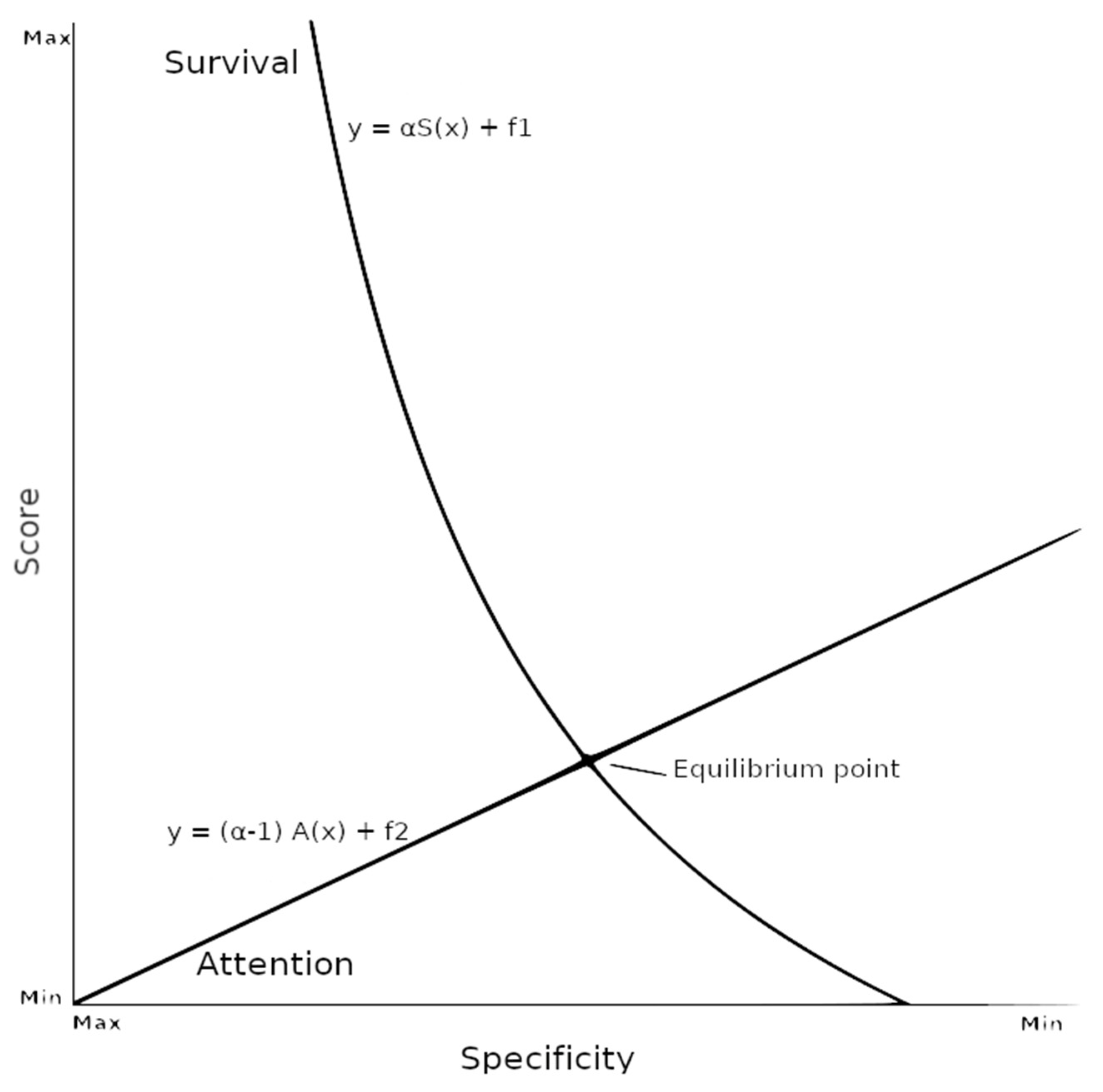
Proposition 1: 

The survival score of a term depends on the specificity of that term inside the ontology structure, so that the more specific a term, the greater the survival score.

Proposition 2: 

The attention level of a term depends on the specificity of that term inside the ontology structure, so that the more specific a term, the less attention it will achieve.

Proposition 3: 

For every term, there is a point where survival and attention intersect, and that is the equilibrium point.

It is trivial to state that when the keyword does not have competitors, the survival score tends to be ∞ (i.e.,$\underset{C\left(k\right)\to 0}{\mathit{lim}} S\left(k\right)=\infty$) as opposed to when we have infinite competitors, where the survival score would be zero (i.e.,$\underset{C\left(k\right)\to \infty }{\mathit{lim}} S\left(k\right)=0$). Concerning the attention score, if a term attracts the attention of infinite competitors, the attention will be at the maximum. In contrast, attention is zero when nobody is interested in that term. Figure 1 graphically represents the equilibrium point. The equilibrium point is the level of specificity where the attention and survival scores intersect. Thus, the closest keyword to the equilibrium point would be the equilibrium keyword.

The equilibrium point depends on various factors, such as the α value and $f_1$ and $f_2$, which refer to the minimum level of keywords and the minimum interest in terms that can be used to find the maximum depth of an ontology.

So, if we choose a more generic keyword than the equilibrium keyword, we are reducing the survival score, and with that, the AS score will also decrease, while choosing a keyword that is less generic than the equilibrium keyword will reduce the AS score due to a reduction in attention.

4.2. Properties

We can use the idea behind the dynamics of supply and demand [27] from econometrics to better understand the behavior of the attention and survival functions. However, we must take into consideration that behavior tends to be slightly different between the two concepts.

5. Attention

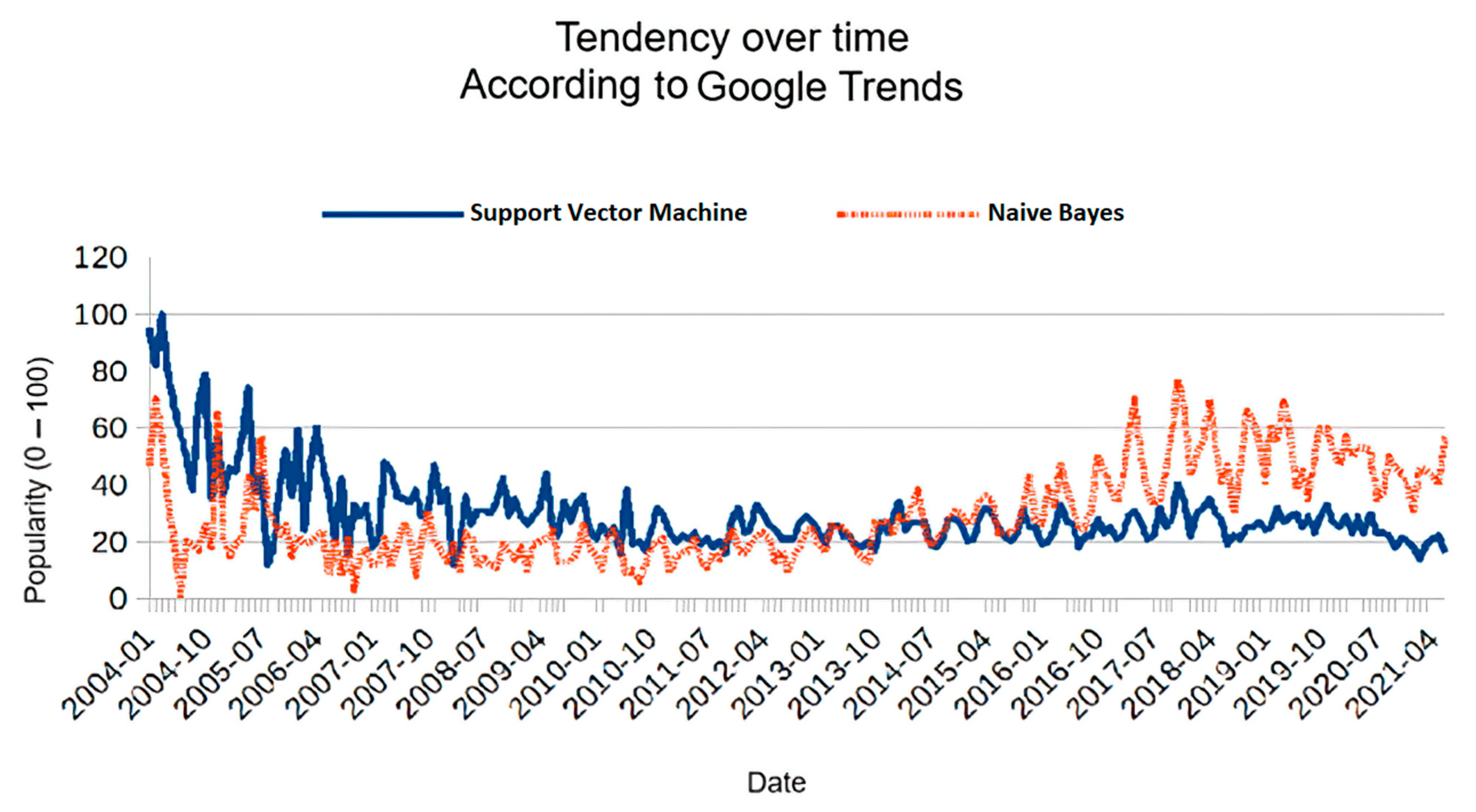
Attention is a dynamic function that fluctuates over time, as it describes the behavior of people. Therefore, the popularity of a keyword is constantly changing. For example, Figure 2 illustrates the behavior of the keyword “support vector machine” vs. “naive Bayes” from 2004 to 2021, according to Google Trends. As we can see, “support vector machine” seems to be surpassed by “naive Bayes” over time. Attention can play the same role as demand in economics theory. We can also interpret demand as the expected income a researcher hopes to receive when using a particular keyword.

A change in the popularity of a keyword produces a variation in the same sign in the attention function.

6. Survival

Survival is also dynamic and changes over time, as it describes the behavior of keywords. Survival can only grow to a certain fixed level based on the finite number of manuscripts that use a specific keyword. The role of survival might be similar to that of supply, but its dynamics are quite different. One approach can be to analyze attention and survival within a specific window of time so that survival would also be able to increase or decrease in response to tendencies. Survival can also be interpreted as the fixed price that a researcher must pay to use certain keywords.

A change in the number of manuscripts that contain a specific keyword produces a variation in the opposite sign in the survival function.

7. Complementary and Substitutive Keywords

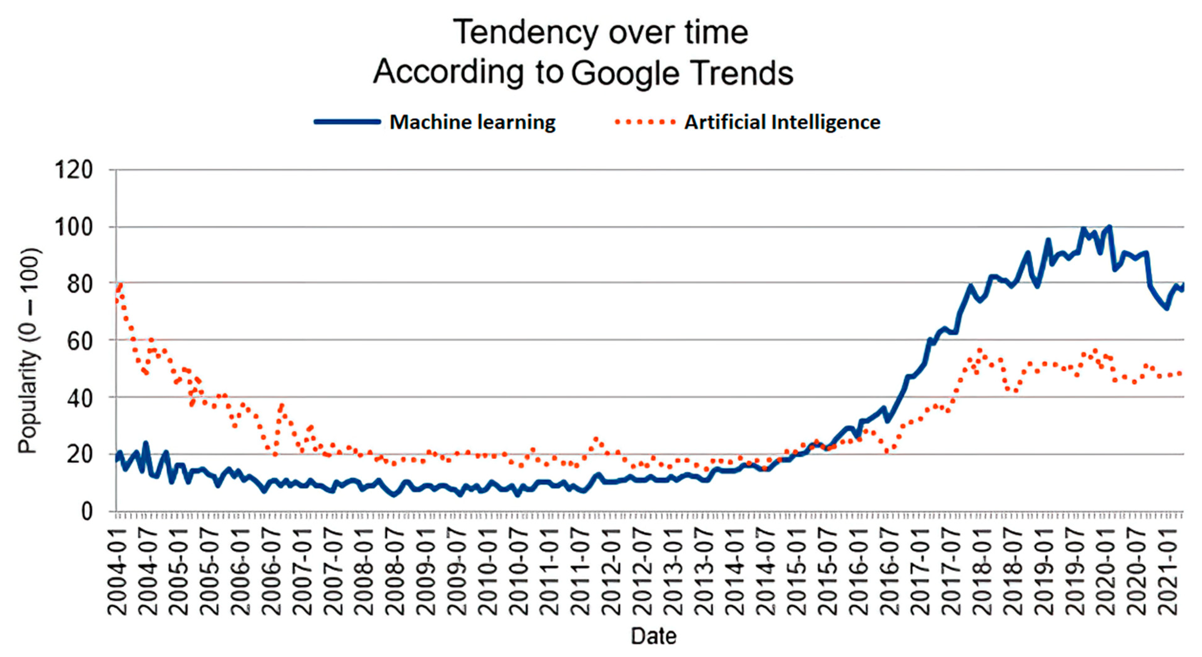
Beyond the relationships so far discussed, it should also be noted that keywords have relationships among themselves as well. In addition, sometimes people start using a new keyword to refer to an existing concept. For example, in economic theory, a complementary keyword is a keyword whose popularity can, in turn, affect the popularity of the related keyword. At the same time, when a complementary keyword is affected in terms of survival, the complemented one is affected in the same way. This relationship is common in the case of synonyms, semantic parents, or children, or keywords significantly correlated to one another. For example, the term “machine learning” is highly connected with the term “artificial intelligence”, according to Google Trends (see Figure 3). With this information, we can see that complementary keywords have a positive correlation. When the complemented keyword gains popularity, the complementary keyword also increases in popularity. When the researcher community increases the use of one keyword, the other keyword also experiences an increase.

If one keyword completely replaces another one, then we are talking about substitutive keywords. When one substitute candidate keyword experiences an increase in attention, the attention received by the replaced keyword decreases. Similarly, when one keyword decreases its survival score, the other one experiences a reduction in the rate that its survival decreases. If we use the window-in-time approach, there is a negative correlation between both keywords’ survival scores. An example of possible substitutive keywords is “support vector machine” vs. “naive Bayes” (see Figure 2) or “C++” vs. “Python”.

As always, it is important to note that correlation does not imply causation. For example, both keywords “Digimon” and “hip-hop” experienced a similar tendency on Google Trends, but there was no clear relationship between these two concepts. While correlation can help us identify associations between keywords, we are required to further analyze the information to make decisive conclusions. For example, ontologies, lists of synonyms and antonyms, or analyses of social trends can help us to identify these associations.

8. Outsiders, Outlier Keywords, and Local Maximums

Not every keyword is part of an ontology relationship. For example, the “Me Too” movement and the hashtag #MeToo have an important attention score [28], and there are many academic manuscripts that use “MeToo” as a keyword [29]. “Me Too”, for example, is an outlier keyword if we are using WordNet, where this concept is not represented.

Often, child concepts have better attention or survival than their parents. For example, “AIDS” has stronger popularity than its parent, “immunodeficiency”, in WordNet. Even if these local maximums’ existence is quite common within the ontology, the general tendency should follow the theoretical model posed in the previous section of our paper.

9. Candidate Generation

We propose an iterative process to improve the attention–survival score of a manuscript’s keywords by using their keyword “neighbors”. To explore the neighborhood, we can use a variety of techniques. In our paper, we propose using ontologies, as we can use human knowledge to determine the meaningful relationships of a keyword. Often, keywords have a very specific meaning, and it is important to change their semantic role as little as possible.

As ontologies are represented and defined as a tree, we must assume a trade-off between being general and being specific. By generalizing, we will often be able to increase the attention score, but it will also increase the size of the community. Thus, an increase in $A\left(k\right)$ will often imply a decrease in $S\left(k\right)$. Conversely, moving to more specific keywords will increase $S\left(k\right)$ and decrease $A\left(k\right),$ as specific keywords are searched for less often than generic ones. For this reason, $\alpha$ and 1-$\alpha$ play an essential role in the refining process.

It is important to consider that ontologies can also contain synonyms (i.e., brother nodes). In relation to synonyms, it is difficult to predict their effects on survival and attention.

Let $g\left(k_i,k_j\right)=\frac{1}{d\left(k_i,k_j\right)}$ represent the benefit of selecting the keyword $k_i$ instead of $k_j$ in terms of the distance between nodes. When $k_i=k_{j}g$, is 1. We define the evaluation function $f\left(k_i,k_j,k_s\right)$ as

$$f\left(k_i,k_j,k_s\right)=AS\left(k_i\right)·g\left(k_i,k_s\right)+AS\left(k_j\right)·g\left(k_i,k_j\right)$$

where $k_s$ is the starting candidate keyword.

We aim to perform an iterative process to discover new candidate keywords and estimate whether paying the distance cost is worth increasing the AS score. Our iterative process is shown in Algorithm 1.

Algorithm 1: Keyword refinement algorithm.

1. We start with an initial candidate set, Kinitial 2. Kcandidates = {Kinitial} 3. For each keyword, k, in Kinitial: 3.1. kstart = k                #kstart is the starting candidate keyword. 3.2. Ksuccessors = {kstart}         #Ksuccessors is the set of potential replacements for kstart. 3.3.         Kqueue = {kstart}      #Kqueue is a queue of candidates that have not been explored yet. 3.4. While Kqueue is not empty: 3.4.1. ksource = next(Kqueue) #gets the element out in front 3.4.2. Kneighbours is the list of neighbours of ksource, including ksource. 3.4.3. ASneighbours is the list of AS scores for each keyword in Kneighbours. 3.4.4. Fneighbours = {ƒ (ksource, kj, kstart) for each kj in Kneighbours) 3.4.5. kbest is the keyword with the maximum ƒ value in Fneighbours. 3.4.6. If kbest is not in Ksuccessors: 3.4.6.1. Ksuccessors = Ksuccessors ∪{kbest} 3.4.6.2. Kqueue = Kqueue ∪{kbest} 3.5. For each keyword, kcandidate, in Ksuccessors: 3.5.1. For each candidate set, Kcandidate_set, in Kcandidates: 3.5.1.1.      We create a new set, Knew_candidate_set by replacing kcandidate by k 3.5.1.2.      Kcandidates = Kcandidates ∪ Knew_candidate_set 4. We return the set in Kcandidates that maximizes the AS score.

10. Toy Example

To illustrate our method, we chose a real paper that only has three keywords: “Chlorofluorocarbons”, “sorption”, and “computer simulation” [30].

The first step is to choose one keyword for the queue iteration, for example, “Chlorofluorocarbons”, and retrieve all its neighbors according to WordNet. Then, for each neighbor, we compute its attention–survival (AS) score as follows, with “Fluorocarbon” being the neighbor with the best score.

• Fluorocarbon → 4.95
• HCFC → 0.000264
• Freon → 1.62
• hydrochlorofluorocarbon → 0.40535
• Chlorofluorocarbons → 0

The next step is to compute ƒ, which considers the gain by moving from the original term to one of its neighbors. In this example, we consider that the benefit of moving to a direct parent, children, or other brother terms in the ontology will always be the same distance, 1. For example, the ƒ value of moving from “Chlorofluorocarbons” to its parent, “Fluorocarbon”, can be expressed as follows:

$$\begin{array}{c}f\left(\mathrm{chlorofluorocarbons},fluorocarbon,chlorofluorocarbons\right)=\\ AS\left(chlorofluorocarbons\right)·\\ ·g\left(chlorofluorocarbons,chlorofluorocarbons\right)\\ +AS\left(fluorocarbon\right)·g\left(chlorofluorocarbons,fluorocarbon\right)\end{array}$$

with

• $g\left(chlorofluorocarbons,chlorofluorocarbons\right)=0$;
• $g\left(chlorofluorocarbon,fluorocarbon\right)=1$;
• $AS\left(chlorofluorocarbons\right)=0$;
• $AS\left(fluorocarbon\right)=4.95;$

Afterwards, we compute ƒ.

$$f\left(\mathrm{chlorofluorocarbons},fluorocarbon,chlorofluorocarbons\right)=0·1+4.95·1=4.95$$

For the first step of the algorithm, retrieving the $f$ values is trivial, as the gain from moving to a direct neighbor is always one, and k_i is the same as k_start, so all $f$ values will ultimately coincide with their AS scores.

$$\begin{gathered} f\left(\mathrm{chlorofluorocarbons},HCFC,chlorofluorocarbons\right)=0.002 \\ f\left(\mathrm{chlorofluorocarbons},freon,chlorofluorocarbons\right)=1.62 \\ f\left(\mathrm{chlorofluorocarbons},hydrochlorofluorocarbon,chlorofluorocarbons\right)=0.41 \\ f\left(\mathrm{chlorofluorocarbons},chlorofluorocarbons,chlorofluorocarbons\right)=0 \end{gathered}$$

“Fluorocarbon” was the best-scored term, so we added “Fluorocarbon” to the candidate set as well as to the queue for the following iteration.

We repeated the process, obtaining “Fluorocarbon” from the candidate set k_i = “Fluorocarbon”. Note that our starting keyword in the algorithm, k_start, is “Chlorofluorocarbons”. When looking for neighbors and scores, we obtained 13 neighbors this time, with “Fluorocarbon” being the best. As “Fluorocarbon” was in the candidate set, we did not add it to the queue iteration.

The next step was to generate new candidate sets from the new candidate keywords. We proceeded by replacing the original keyword with the new candidate one. Thus, our new list of candidates was as follows:

{“Chlorofluorocarbons”, “sorption”, and “computer simulation”}

{“Fluorocarbon”, “sorption”, and “computer simulation”}

The next keyword to refine was sorption, which only had one good neighbor, “attention”. This meant we needed to add it to the new candidate sets:

{“Chlorofluorocarbons”, “sorption”, “computer simulation”}

{“Fluorocarbon”, “sorption”, “computer simulation”}

{“Chlorofluorocarbons”, “attention”, “computer simulation”}

{“Fluorocarbon”, “attention”, “computer simulation”}

Finally, it was time to refine “computer simulation”, which was a local maximum, meaning that this term did not have any neighbors with an AS score higher than its own AS score, so we did not add any new candidate sets. In conclusion, the best scored candidate set was {“Fluorocarbons”, “attention”, “computer simulation”}.

This entire process was firmly based on the knowledge from the ontology used (in our case, WordNet) and should be seen as a decision support system to help humans refine their keywords’ impact. In the example, “Chlorofluorocarbons” was replaced by “Fluorocarbon”, which is a more generic concept that includes all “Chlorofluorocarbons”. Authors must then judge whether it is worth the cost to accept the loss of specific information to use a more attractive keyword for the audience.

In the case of “attention”, “sorption” is the generic form of “absorption”, so our algorithm moved to a child concept in order to finally end up with “attention”, which is another meaning of the keyword “absorption”. In the context of the article, it seems that “attention” is not a good choice to replace “sorption”, because the manuscript context seems to be related to chemistry, not concentration. In this case, maybe the author would prefer to keep “sorption” or replace it with “absorption”, which is a slightly more competitive term that receives more attention.

11. Experimental Design

11.1. Theoretical Model Validation

11.1.1. Data Source

To corroborate the validity of our proposals and gain a better understanding regarding the behavior of attention and survival in an ontology, we extracted data from a few different ontologies: WordNet [31] and the Computer Science Ontology (CSO) [32]. WordNet is a lexical database that gathers words into groups of cognitive synonyms and defines relationships in terms of hypernymy and hyponymy. Thus, despite not being strictly an ontology, we can benefit from the WordNet structure, which also resembles the form of a tree, where each concept is a node.

For its part, CSO is an ontology automatically generated from 16 million publications focused on the computer science field. The CSO model includes eight different semantic relations (relatedEquivalent, superTopicOf, contributsTo, preferntialEquivalent, rdf:type, owlSameAs, and schema:relatedLink). We only used the first two relations mentioned.

All terms from the ontologies are lightly preprocessed to avoid ambiguity and to prepare them to be sent to the APIs in a proper format. The preprocessing steps are the following:

• Replace “-“ and “_” with spaces.
• Remove all characters, except letters, spaces, and “&”.
• Replace “&” with “and”.

For extracting the number of papers according to Scopus, we used the Scopus Search API (Elsevier Developer Portal: https://dev.elsevier.com/ (accessed on 29 March 2023). We sent requests to the Scopus Search API using the following filters:

• We looked for terms inside the keywords’ list of manuscripts: KEY(“term”);
• We filtered all manuscripts, except articles, reviews, and conference papers. DOCTYPE(“ar”), DOCTYPE(“re”), DOCTYPE(“cp”).

An example of a query search is as follows:

KEY (‘SCIENCE’) AND (LIMIT-TO (DOCTYPE, ‘ar’)

OR LIMIT-TO (DOCTYPE, ‘re’) OR LIMIT-TO (DOCTYPE, ‘cp’))

From Google Trends, we extracted the popularity results per country and computed the average popularity.

We aimed to analyze the differences between a generic source of terms such as WordNet and a more specific collection related to the computer science field. Scopus provided us with information on the number of papers per keyword necessary to infer survival, while Google Trends gave us information regarding the attention and popularity of a term. Unfortunately, it is important to state that extracting information from a specific academic search engine such as Google Scholar was impossible. Instead, Google Trends gave us results for Google Search, which is used by the general population. Nevertheless, using results from Google can provide us with additional information, such as altmetrics and the social interest in science topics. This paper used attention as an alternative to the topic popularity (TP) measure.

11.1.2. Ontology Analysis

Our purpose was to map the terms in our datasets onto the ontology structure as defined by WordNet and CSO. Before mapping terms, we first wanted to perform an exploratory task on both WordNet and CSO to explore the ontologies’ behavior and clarify whether the theoretical process of attention and survival metrics over an ontology was close to our assumptions. WordNet consists of different synsets outside a hierarchy, but we only studied those connected to the root synset (i.e., entity). A synset can have one or more lemmas, so we used the median value of the attention and survival scores across all lemmas. Using the median value instead of the mean to determine the score of a synset is based on the fact that the distribution scores of lemmas tend to present a skewed result. However, we used the mean attention and survival numbers to compute the scores per level.

Table 1. Scopus and Google scores per depth level in WordNet. All values are the average scores of each synset with the same distance to the root node, and the value of each synset was computed by considering the median value of all lemmas within the synset. Note that level 1 only has the root synset.

Scopus and Google Scores in WordNet Ontology
Level	Scopus	Google
1	22,823.0	5.504
2	13,961.5	2.756
3	39,043.0	3.626
4	31,037.5	3.538
5	1203.0	2.608
6	263.0	2.160
7	95.0	1.900
8	49.0	1.676
9	34.5	1.580
10	25.0	1.494
11	11.5	1.200
12	9.5	1.044
13	10.0	0.836
14	11.5	0.776
15	16.0	0.774
16	17.3	0.920
17	14.8	0.882
18	3.0	0.544
19	16.5	1.044

shows the distribution of the Scopus and Google values’ overall levels of depth in WordNet (α = 0.5). We only analyzed depth levels that were greater than five, because, for prior levels, the number of synsets was reduced too much, which could lead to incorrect conclusions and inconsistent results.

After computing the attention and survival scores and extracting the mean values per level, we noted that the scores were on different scales, so we needed to perform a min–max normalization to keep all values in the same range [0, 1]. We did this to make the analysis of the effect of both scores in the ontologies more accessible.

Figure 4 shows the survival and attention score evolution across the WordNet structure (α = 0.5). As we can see, survival starts close to 1.0 at depth 17 and is in a continuous decline until being surpassed by attention at level 6, where the equilibrium point is located. Meanwhile, attention continually grows until it reaches its maximum value at level 2. The equilibrium point is located at the coordinates (6.38, 0.48), that is, in level 6, producing an AS score of 0.48, while the maximum score is achieved at level 2, with an AS score of 0.62.

If we check the results from Table 1, we can see that the average number of articles per level is significantly reduced until level 7, while attention tends to grow uniformly.

The observed behavior over the WordNet ontology is in consonance with our proposals. Moreover, we have empirically corroborated that more specificity is related to low attention and high survival scores.

Concerning the WordNet dynamic, we can see how most depth levels contain very specific terms, which are quite unattractive according to Google searches and the number of articles retrieved by a Scopus search.

From these results, one should not deduce that the best option is to choose keywords from levels 7 or 2. WordNet is a generic ontology that contains many terms that are not common in the academic field. Therefore, a domain-specific ontology would be a better option for choosing keywords. A good approach could be to choose an ontology according to the criteria described by [33] (for example, the authors mention clarity, consistency, conciseness, expandability, correctness, completeness, minimal ontological commitment, and minimal encoding bias, among other criteria). Our purpose in employing WordNet was to use a generic and widely validated ontology to analyze the distribution of attention and survival scores.

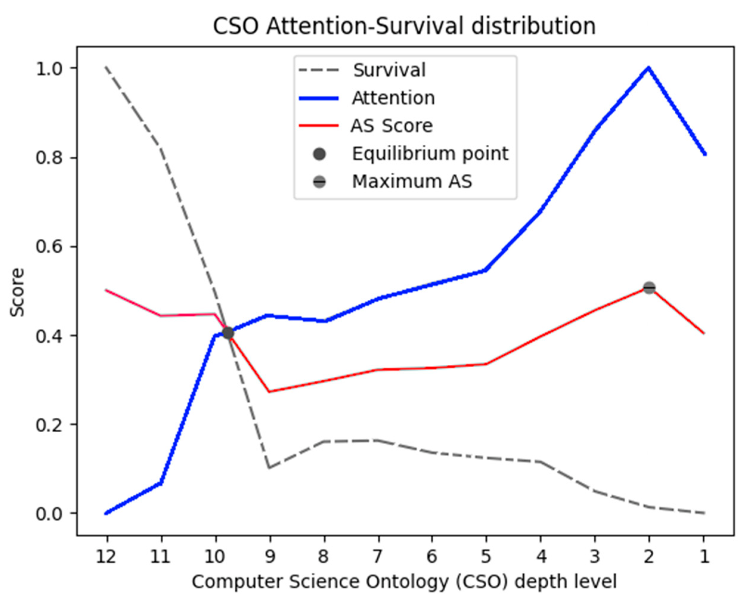
The case for CSO is illustrated in Figure 5.

In CSO, the equilibrium point was reached at level 10, while the maximum AS score was at level 2. In CSO, survival fell very fast, while attention had both fast-growing periods and periods of slow growth. In CSO, the equilibrium point score was very close to the maximum value of AS (the difference was less than 0.02).

Both ontologies show a sudden drop on the first level. It is important to state that the first level is not the root node, which was removed from our data. The upper levels of both ontologies contained such few words that their result could introduce noise into the graph and, thus, should be carefully interpreted.

11.1.3. Keyword Refinement

In this section, we randomly chose keywords from 20 manuscripts, and we ran them through Algorithm 1. The attention results came from Google Trends and were normalized with the interval [0–100] for this refinement process. Thus, we did not need to perform a normalization step.

We limited the distance to the target keywords to two levels to prevent large differences in their conceptual meanings.

11.1.4. WordNet and CSO Refinements

Table 2. List of the different words before and after refining, using WordNet and CSO as ontologies. (An extended version of Table 2 can be found in the Supplementary Materials of this paper.)

	Word Refinements: WordNet and CSO
Initial Word	WordNet Refinement	CSO Refinement
robotics	robotics	robots
telecommunication_equipment	television	sensors
electromagnetism	acoustics	electromagnetic
memory_access	memory_access	memory_access
computer-aided_design	software	computer-aided
gateway	gateway	routing_protocols
lexical_database	lexical_database	artificial_intelligence
speckle	speckle	radar
data_mining	data_processing	clustering
computer_science	plan	software
ergonomics	technology	human_computer_interaction
cosmic_microwave_background	cosmic_microwave_background	polarimeter
buffer_storage	fund	bandwidth
white_noise	impediment	white_noise
relational_database	relational_database	database
electrical_energy	AC	electrical_energy
mobile_phone	cell	sensors
binoculars	binoculars	binocular
object-oriented_programming	hack	java
user_interface	CLI	sensors
authentication	validation	security_of_data
remote_control	device	robotics
spline	remove	computer-aided_design

shows real examples of the author’s keywords refined using WordNet and CSO ontologies (An extended version of Table 2 can be found in the Supplementary Materials of this paper). Keywords were randomly selected from the intersection of the terms contained in both ontologies. As CSO is generated from academic literature, all keywords in the example are real keywords. Many keywords were not replaced by others. This can happen for two reasons: The algorithm is limited to exploring at only a distance of two; or, if the neighbors’ attention–survival score is low, the algorithm decides not to replace the keyword.

On the other hand, if the keyword is not defined in the ontology, then we cannot use this ontology to refine the keyword, as we do not have enough information about the neighborhood. For WordNet, the distance between terms is provided by the path distance similarity, a metric that denotes how similar two synsets are based on the shortest path that connects the two nodes. This metric is provided by the Python Natural Language Toolkit (NLTK) library https://www.nltk.org/ (accessed on 29 March 2023). For CSO, we determined the distance between two words using the lowest common ancestor (LCA) algorithm [34].

As we mentioned before, WordNet is probably not the best option for use as an ontology, and a knowledge-specific ontology should be used instead (e.g., CSO for computer science or the Ontology for Biomedical Investigations for biological or medical domains) [35]. We can see some replacements of keywords that perhaps are not the best option for manuscripts (Correspondence → card, Testing → Watch …).

The best way to use our method is inside an interactive system that allows the author to know the survival and attention scores from specific keywords and propose alternatives. Of course, the author should always make the final decision.

11.1.5. WordNet and CSO Hierarchy

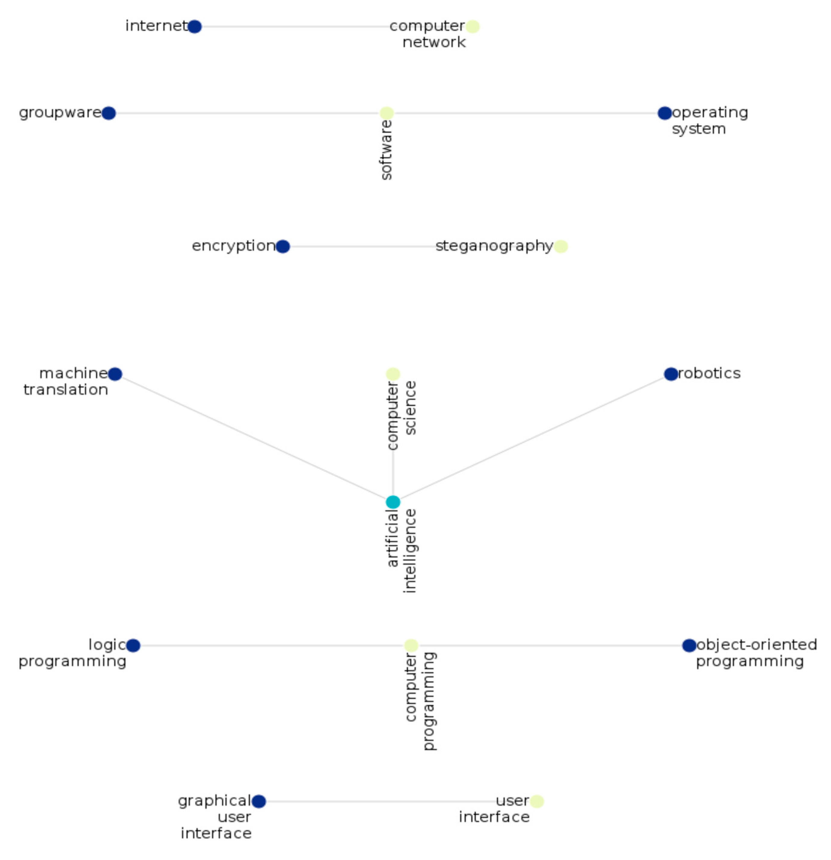
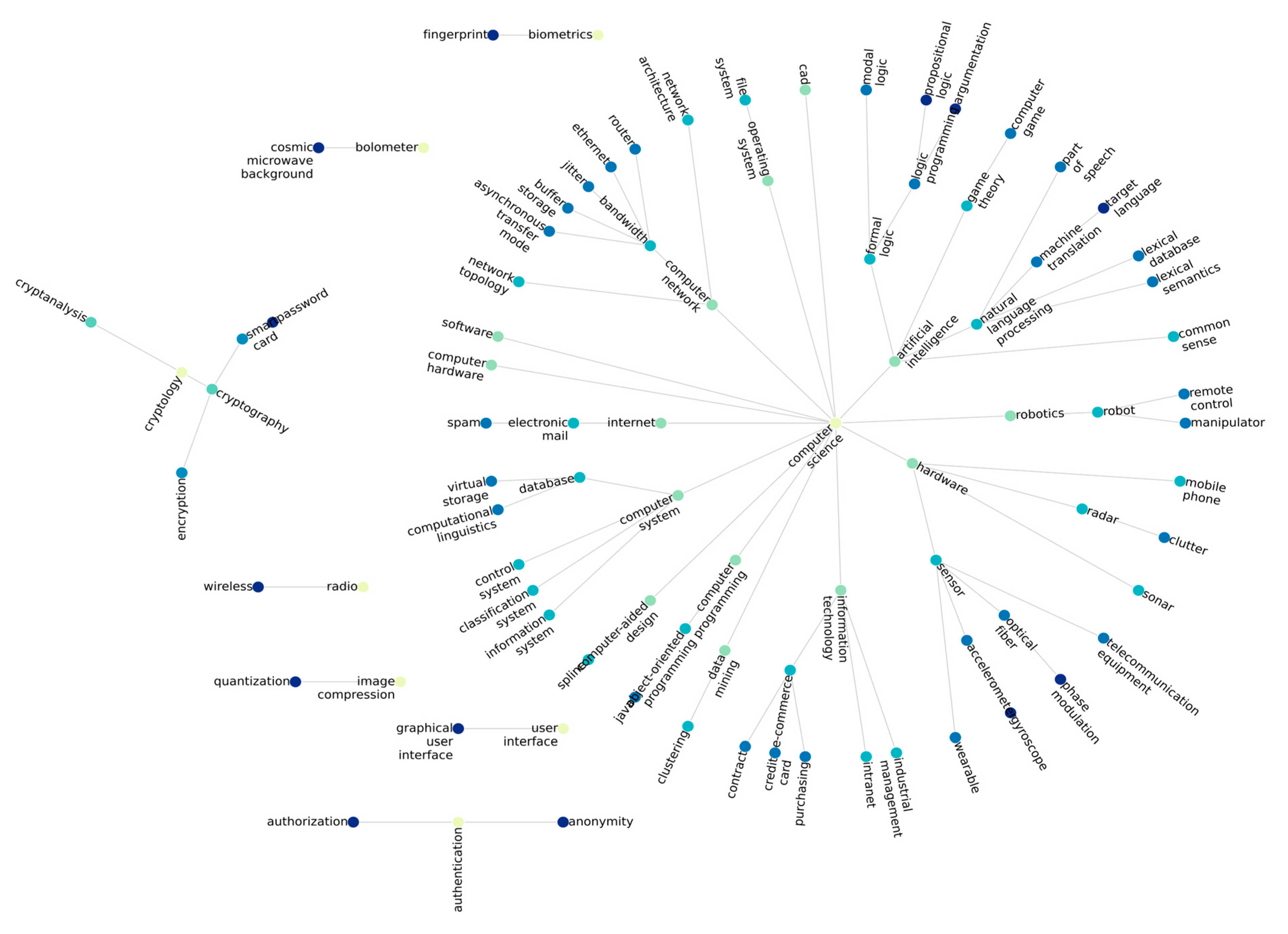
WordNet and CSO have different purposes as ontologies. While some terms are present in both ontologies, the knowledge structure is different between them. This can generate very different results from one ontology to another, as reflected in Table 2. In our paper, we also compared the hierarchy of both ontologies. Figure 6 and Figure 7 present the structure of the same set of keywords according to both the WordNet and CSO ontologies.

As these terms are included in both ontologies, we can assume that these keywords are closely related to the computer science field. Since CSO is an ontology focused on computer science terminology, we can see how these keywords are connected to one another and have fewer isolated nodes. For WordNet, however, most of these keywords are completely isolated, and there are no strong clusters of keywords. Therefore, CSO represents terms with a greater granularity than WordNet, and this situation directly impacts the refinement algorithm.

12. TF-IDF

TF-IDF is probably the most popular measure to determine the relevance of a term inside of a corpus. In this work, we propose an alternative measure of popularity. In the following, we have listed some differences between the attention–survival score and TF-IDF.

• Static vs. dynamic: TF-IDF, applied over a corpus, is a static measure that is not liable to change, while attention–survival is updated in real time. Even when applied over a static corpus, attention–survival will return a score that represents the current popularity of a measure according to the social attention given to a particular term. For this reason, the AS score is a recommended alternative to positioning a term, taking into consideration the social behavior of a community around a term.
• Source of information: while TF-IDF relies on statistical information about the distribution of a term in a corpus, AS extracts its information from both statistical and temporal data.
• Type of information: On the one hand, TF-IDF is a technique that comes from the text mining field. This means it requires a corpus to extract the popularity score. On the other hand, the AS score does not require a corpus of text for it to work. It would be a suitable measure to categorize multimedia information, such as videos or photos.

Alternative Popularity Measures

As mentioned before, Google Trends provides information regarding the general behavior of Internet users instead of the habits of researchers. [36] propose a measure named topic popularity (TP), which is represented as follows:

$${TP}_Y^p={{\displaystyle \sum }}_m{{\displaystyle \sum }}_n{top}_{m,n}·{\theta }_m^p·{\phi }_n^m$$

where $p$ is an article, Y is the year, $M$ is the number of LDA topics, $N$ is the number of keywords ($m\in \{1,2,\dots ,M\}$, $n\in \{1,2,\dots N\}$), ${\theta }_m^p$ is the probability of topic $m$ occurring in paper $p$, ${\phi }_n^m$ is the probability of keyword n occurring in topic m, and ${top}_{m,n}$ is the number of questions retrieved by ResearchGate.

We aimed to analyze the differences between the Google Trends score and topic popularity. On the one hand, topic popularity collects data from ResearchGate (to collect data from ResearchGate, we used the online search engine Microsoft Bing, filtering by the domain researchgate.net), an academic source of scientific information. This guarantees that the popularity is not biased by data from outside of the scientific community, which is the main disadvantage of Google Trends. On the other hand, Google Trends represents popularity from the present, as it is based on current searches from the Internet, while ResearchGate could be counting information from the past (the minimum temporal unit of time used by ResearchGate is the year).

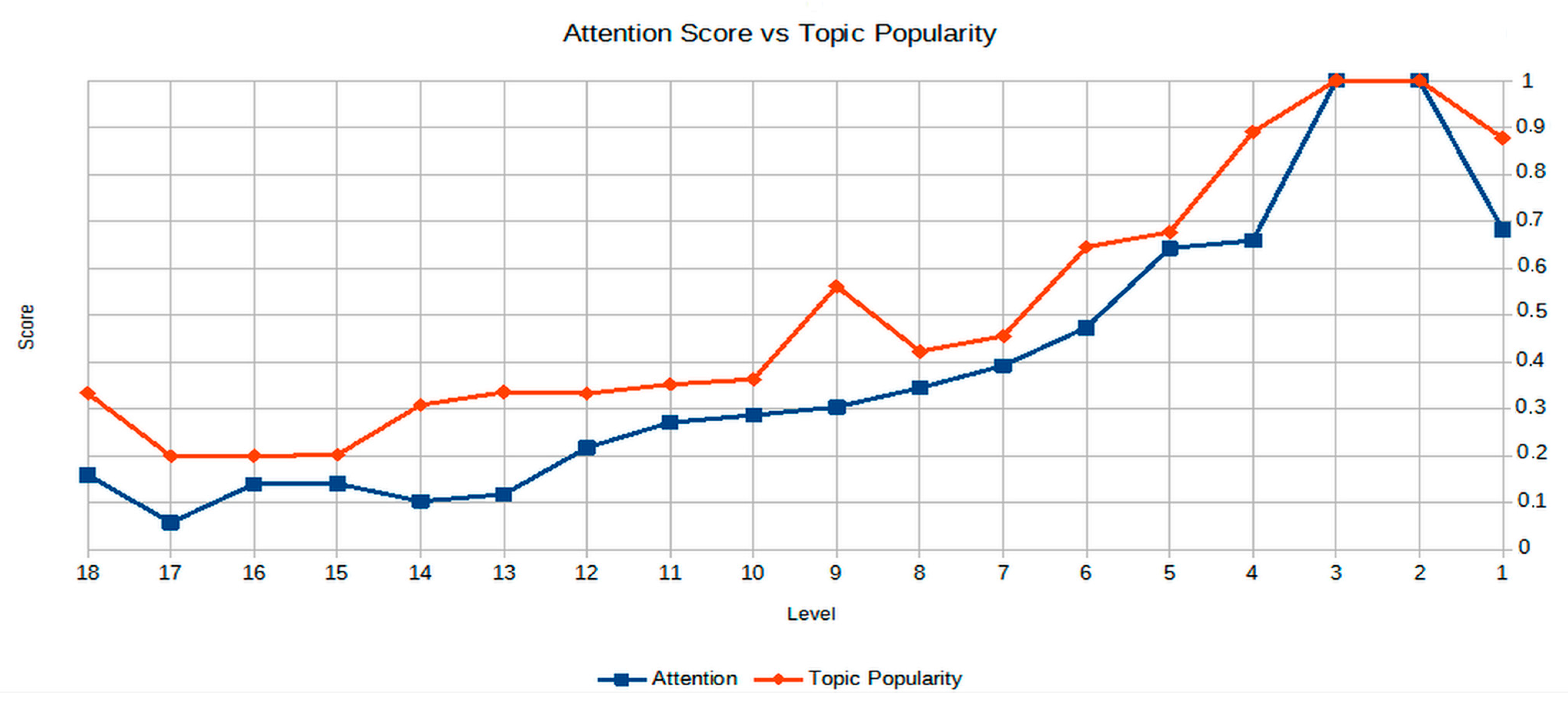
To perform the comparison, we used the same dataset mentioned in Section 11.1.1, “Data Source”, but we extracted the title and abstract from the articles and applied the LDA model, as described by the authors in [36]. First, we defined 100 LDA topics with an asymmetric alpha parameter; after, we selected 400 random words from WordNet and used them as a target keyword, computing the topic popularity and attention score for 2022. The results are shown in Figure 8. According to our results, TP always obtained higher attention values. This result can be explained by the fact that specific computer science terms are used more often by the academic public than a general audience. On the other hand, ResearchGate retrieves documents, links, and information generated before 2022 but uploaded in 2022, while Google Trends always shows results from 2022. Nevertheless, both metrics show a similar tendency, where popularity and attention decrease at higher WordNet levels.

13. α Parameter

The α parameter allows us to calibrate the attention and survival scores.

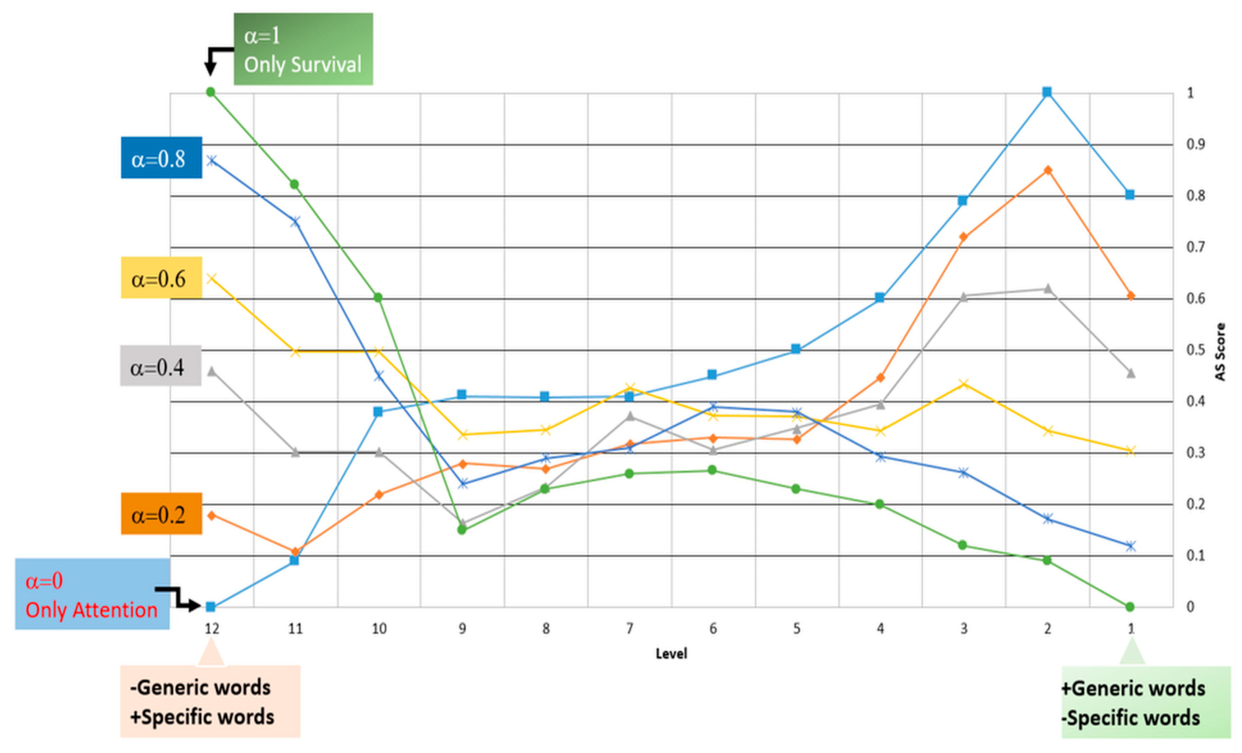
Figure 9 represents the value of the AS score obtained with the words in the CSO ontology at different depth levels. Thus, at level 1, the words were more generic and less specific. At level 12, they were less generic and more specific. Figure 9 shows the analysis of the behavior of the AS score for different α values.

When α = 0, we only consider attention, while only survival is considered when α = 1. The green line in Figure 8 represents a low level with less specificity, and the survival score was low, whereas, at a high level, the score achieved the highest value. In addition, the blue line in Figure 8, with the opposite behavior, represents the attention score.

From Figure 8 and setting a word-depth level, the most appropriate α can be chosen to maximize the AS score. Thus, for example, if the level of the words is 7, looking at Figure 8, the most suitable α would be equal to 0.6.

Moreover, by analyzing Figure 8, we can characterize the words of the CSO ontology. As shown, the words from level 1 to level 9 present a substantial attention value, meaning that they are generic words and are frequently used. At a depth level of 10, the words in the ontology are returned with a higher attention value, indicating that they are more specific.

Figure 8 also confirms Propositions 1, 2, and 3. Thus, for example, for α = 1, the green line shows that high survival values correspond to greater specificity (Proposition 1). At the same time, low survival values correspond to a lower specificity. In addition, when also analyzing the signal for α = 0, where only the attention component is active in the AS score, high specificity values correspond to low attention values. Following Proposition 3, the equilibrium point would be between levels 9 and 10.

14. Refinement Algorithm Validation

To validate Algorithm 1, we launched three experiments to test the adequacy of our model.

Experiments 1 and 2 used a survey to receive feedback from human subjects. The survey in both experiments was the same, but the target participants were different.

14.1. Survey Preparation

First, we extracted 500 articles from the Web of Science by selecting articles with the query “Computer Science”, including only papers. The complete dataset can be found at Kaggle https://www.kaggle.com/datasets/jorgechamorropadial/scie-2019 (accessed on 29 March 2023). The keywords from selected articles have been refined using Algorithm 1.

To deal with unknown terms, we first looked at CSO, which is the ontology most related to the computer science dataset we used. If the keyword was not present in CSO, we the tried to find the concept in WordNet. When WordNet also failed, DBpedia https://www.dbpedia.org (accessed on 29 March 2023) was used as a last attempt. Finally, if the term was not present in any ontology, we discarded the article and chose another one.

After obtaining a set of refined articles, we randomly chose ten papers to include in our survey. For each selected manuscript, we created a question in the survey where participants were allowed to see the title and abstract of the article and a table with two columns: one for the original set of keywords and another for the refined set. The user had to select one of the following answers:

• R1: The refined set can describe the title with almost the same precision as the initial set;
• R2: The refined set cannot describe the title with almost the same precision as the initial set.

The Supplementary Materials contain all questions asked in the survey.

14.2. Experiment 1: Survey for Nonexperienced Users

Our survey was completed by 51 participants from Amazon Mechanical Turk. The participants were economically reimbursed for their participation and had to meet the following preliminary requirements:

• Live in an English-speaking country;
• Have a bachelor’s degree;
• Work experience in IT.

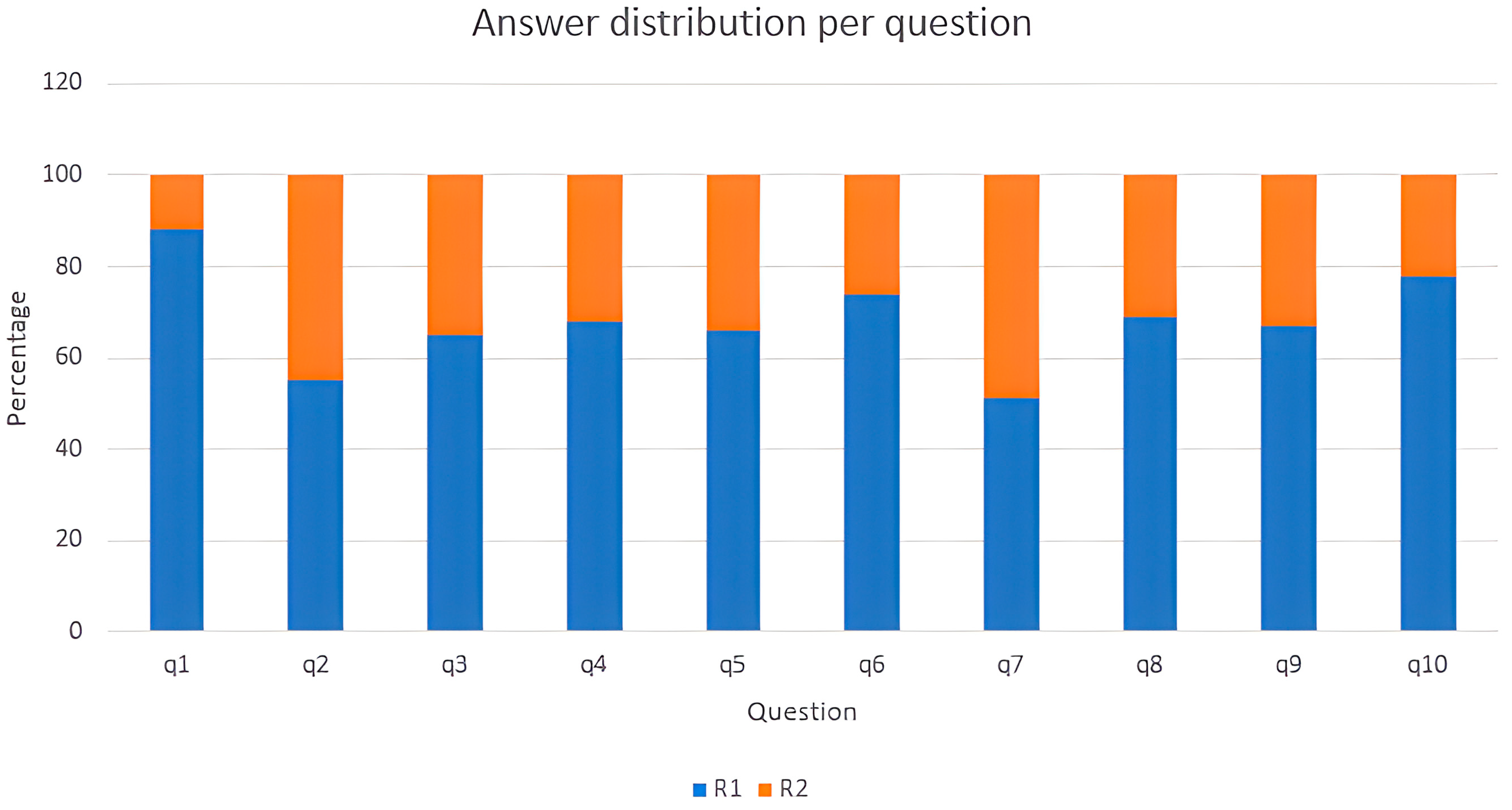
Regarding the survey results, for all questions, most users answered R1. Figure 10 describes the results obtained per question. The worst performance was obtained for q7, where 50.98% of the participants chose R1, while the best results were obtained for q1, where 88.24% of the participants chose R1. In the entire survey, the answer R1 was chosen by 67.85% (standard deviation: 10.43).

Five participants chose R1 for all questions, while nobody selected R2 more times than R1. In global terms, the participants chose R1 for 6.78 questions (standard deviation: 1.62).

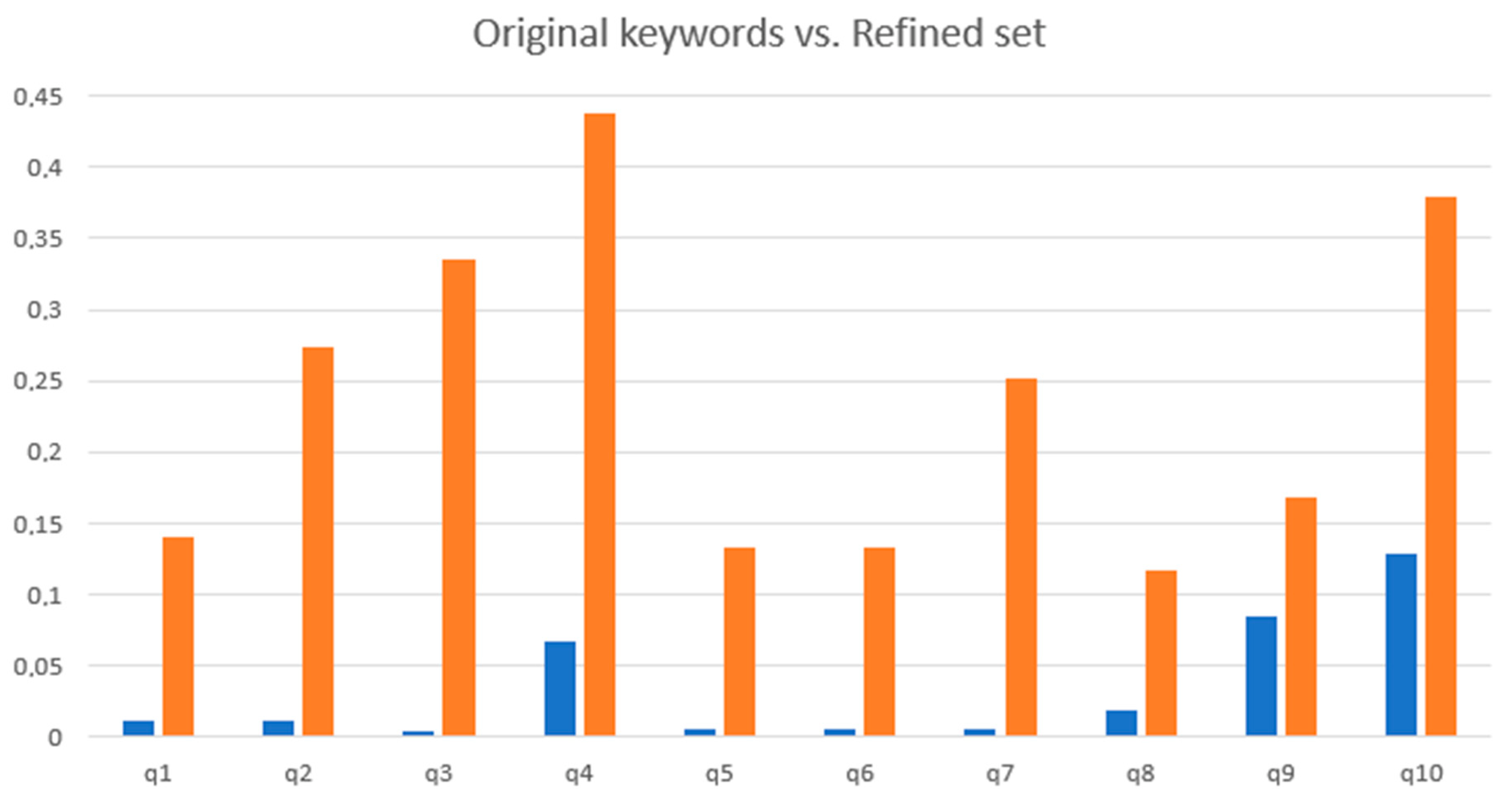
As shown in Figure 11, the refined set of keywords deeply improved the AS score compared to the initial ones. The average improvement ratio is 22.5644 (standard deviation: 24.06).

14.3. Experiment 2: Survey for Experienced Users

Participants had to meet the following preliminary requirements:

• Live in an English-speaking country or have a C1 level of English according to The Common European Framework of Reference for Languages or higher;
• A master’s thesis and a minimum of two scientific publications;
• Work experience in IT or in research.

Our survey was completed by 46 participants. A set of demographic questions were presented, with the following responses:

• English level:

  o

  Nineteen participants lived in an English-speaking country or had a native level of English;

  o

  Twenty-four participants had a C1 level or equivalent;

  o

  Three participants had a C2 level.

• Education:

  o

  Twenty-five participants completed a master’s thesis;

  o

  Twelve participants had a PhD;

  o

  Nine participants were university professors or researchers.

• Background:

  o

  Thirty-two participants had two scientific publications;

  o

  Fourteen participants had more than two scientific publications.

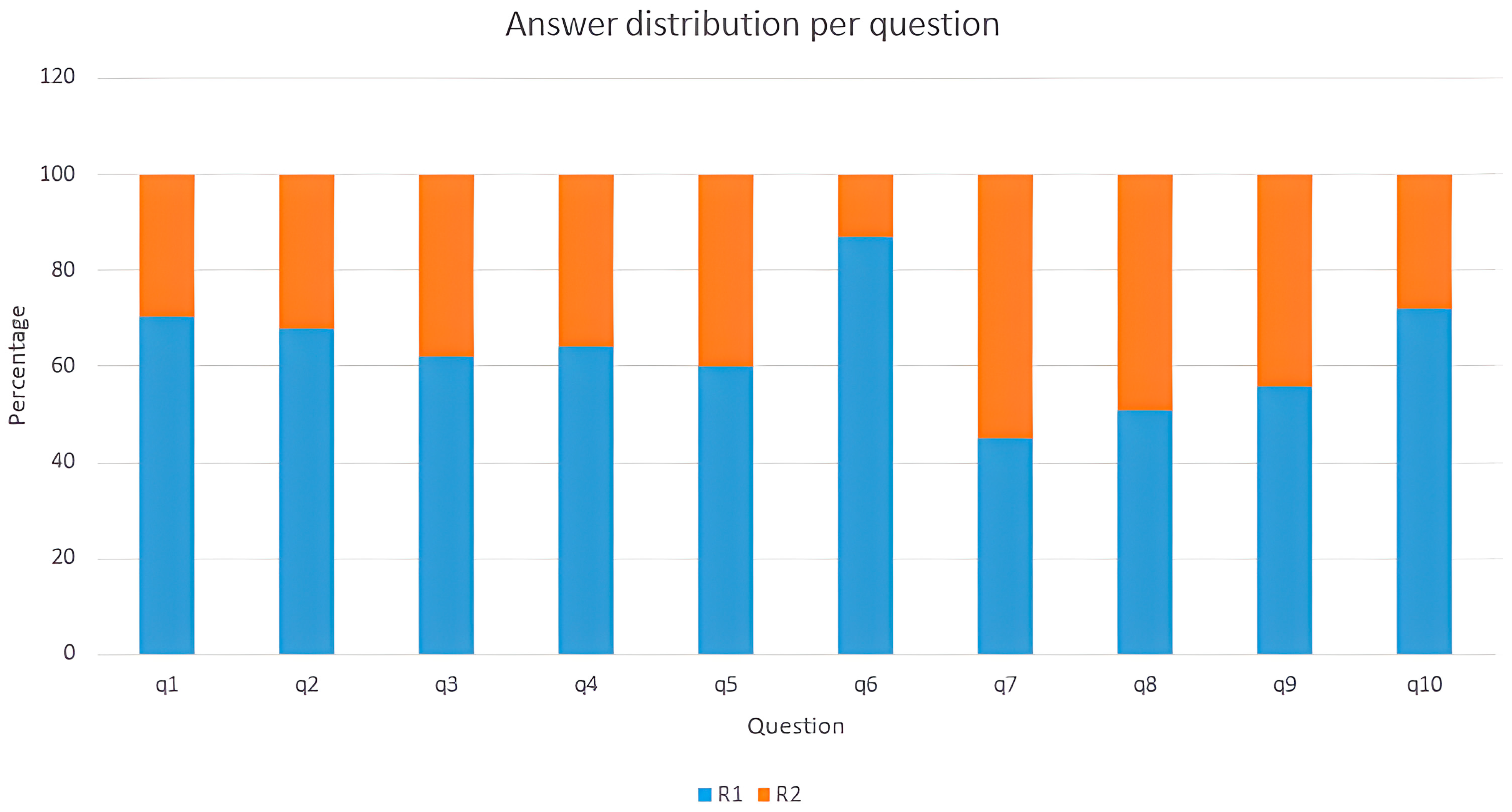
With respect to the survey results, for all questions, most of the users answered R1. Figure 11 describes the results obtained per question. The worst performance was obtained for q7, where 45.20% of the participants chose R1, while the best results were obtained for q6, where 87.95% of the participants chose R1. In the entire survey, the answer R1 was chosen by 63.52% (standard deviation: 11.82).

Three participants chose R1 for all questions, while nobody selected R2 more times than R1. In global terms, participants chose R1 for 6.20 questions (standard deviation: 2.01).

As we can see in Figure 12, the refined set of keywords deeply improved the AS score in comparison with the initial ones. The average improvement ratio was 22.5644 (standard deviation: 24.06).

14.4. Experiment 3

For this experiment, we randomly selected 330 articles from the same dataset downloaded for the survey. For each article, every keyword had a 50% probability of being changed by another term that was related but with a lower AS score.

After changing the keywords of the 30 articles, we applied our algorithm to each of them and checked the intersection over union (IoU) metric. IoU is defined as follows:

$$IoU=\frac{\mathrm{P}\mathrm{r}\mathrm{o}\mathrm{p}\mathrm{o}\mathrm{s}\mathrm{e}\mathrm{d} \mathrm{k}\mathrm{e}\mathrm{y}\mathrm{w}\mathrm{o}\mathrm{r}\mathrm{d}\mathrm{s}\cap \mathrm{O}\mathrm{r}\mathrm{i}\mathrm{g}\mathrm{i}\mathrm{n}\mathrm{a}\mathrm{l} \mathrm{K}\mathrm{e}\mathrm{y}\mathrm{w}\mathrm{o}\mathrm{r}\mathrm{d}\mathrm{s}}{\mathrm{P}\mathrm{r}\mathrm{o}\mathrm{p}\mathrm{o}\mathrm{s}\mathrm{e}\mathrm{d} \mathrm{k}\mathrm{e}\mathrm{y}\mathrm{w}\mathrm{o}\mathrm{r}\mathrm{d}\mathrm{s}\cup \mathrm{O}\mathrm{r}\mathrm{i}\mathrm{g}\mathrm{i}\mathrm{n}\mathrm{a}\mathrm{l} \mathrm{K}\mathrm{e}\mathrm{y}\mathrm{w}\mathrm{o}\mathrm{r}\mathrm{d}\mathrm{s}}$$

where Proposed Keywords are the new keywords suggested by the algorithm, and Original Keywords is the original set of keywords chosen by the article’s authors.

We obtained the following results:

• IoU score: 0.594 (standard deviation: 0.307);
• Precision: 0.694 (standard deviation: 0.261);
• Recall: 0.696 (standard deviation: 0.258);
• Accuracy: 0.690 (standard deviation: 0.265);
• F1 score: 0.69 (standard deviation: 0.100);
• Rate of changed keywords: 0.431.

Note that not every keyword is susceptible to being changed. Keywords were not replaced if they were not defined in any of the three ontologies (WordNet, DBPedia, and CSO), even if they should be modified because of the probability.

15. Future Work

Apart from the theoretical model tested in this work, as well as the three experiments performed and described below, the algorithm is expected to be put into production in order to serve other researchers and general users in an intuitive way. For this reason, a web application is being built to provide users with an intuitive and interactive user interface. The application is being designed to support the most common ontology formats (e.g., n3, owl, and xml) and is expected to be published in future work along with more experimental results to examine the performance of our algorithm.

16. Conclusions

Typically, keywords are selected by an author’s intuition, or sometimes without applying any method at all. This can lead to bias, errors, and loss of opportunity.

The goal of our paper was to emphasize the importance of knowing the results of choosing different keywords. Choosing a keyword implies putting a future manuscript in competition with others, which all work to gain a certain amount of attention from the community that varies and depends on external factors. For this reason, keywords are constantly changing in terms of attention and survival rates. Concerning survival, we can conclude that all keywords decrease their survival possibilities over time. However, in general terms, survival tends to decrease when moving from specific concepts to generic ones. At the same time, attention tends to decrease when moving from generic terms to specific ones. Sometimes, attention and survival intersect at certain equilibrium points. A keyword with both survival and attention scores that are simultaneously high characterizes a keyword that will be used across time and will continue to be of interest to the community. To establish the survival and attention values of a keyword, we defined the AS score.

We presented an algorithm to refine keywords using ontologies to find alternative keywords with high survival and attention scores. Ontologies can be used as an essential source of knowledge that can help us organize keywords along the generic–specific axis. We analyzed WordNet and the Computer Science Ontology (CSO), both ontologies but with different backgrounds. CSO is a field-specific ontology, while WordNet provides good comparison data to examine how our model works.

Implicitly, our method uses state-of-the-art strategies to reduce the probability of choosing a poor keyword [3,9] thanks to the implementation of ontologies and the possibility of moving into general or specific terms, according to the score obtained through the concept hierarchy.

Another important topic is human validation. We performed a survey where 51 participants answered positively in relation to the results attained using our algorithm, which used WordNet, CSO, and DBpedia as ontological sources.

Our method can be generalized and applied to other fields, for example, marketing. In addition, it can be helpful as a system to extract keywords when text mining is not an option, for example, if we want to categorize images or videos.

In conclusion, it is important to state that our algorithm is intended to provide authors with additional information regarding how to choose keywords for a manuscript and to propose suggestions. However, the author is ultimately responsible for making the decision. Finally, our algorithm is not a keyword suggester; if an author makes a bad decision in choosing a keyword, the refinement process likely will not help very much because it can only explore the related context of a keyword. In that case, the author must use some other methodology or information to select a good starting keyword candidate set.