Stochastic Safety Radius on UPGMA

Abstract

Unweighted Pair Group Method with Arithmetic Mean (UPGMA) is one of the most popular distance-based methods to reconstruct an equidistant phylogenetic tree from a distance matrix computed from an alignment of sequences. Since we use equidistant trees as gene trees for phylogenomic analyses under the multi-species coalescent model and since an input distance matrix computed from an alignment of each gene in a genome is estimated via the maximum likelihood estimators, it is important to conduct a robust analysis on UPGMA. Stochastic safety radius, introduced by Steel and Gascuel, provides a lower bound for the probability that a phylogenetic tree reconstruction method returns the true tree topology from a given distance matrix. In this article, we compute the stochastic safety radius of UPGMA for a phylogenetic tree with n leaves. Computational experiments show an improved gap between empirical probabilities estimated from random samples and the true tree topology from UPGMA, increasing confidence in phylogenic results.

1. Introduction

Phylogenetics is one of the oldest fields in biology to study the evolutionary history of organisms using a phylogenetic tree, which is a tree representation of evolutionary history among species (or taxa). In order to reconstruct a phylogenetic tree from genetic data, researchers develop many statistical methods including maximum likelihood estimators, Bayesian inference, and distance-based methods [1]. A distance-based method is one of the most popular methods to reconstruct a phylogenetic tree for its computational speed and relatively simple two-step procedure: (1) computing all pairwise distances between all possible pair of sequences from the input alignment; and (2) reconstructing a phylogenetic tree from all pairwise distances of sequences computed in Step (1) using combinatorics.

Maximum likelihood estimators under evolutionary models produce pairwise distances between all possible pairs of sequences and they form as a distance matrix. A distance matrix is an input for a distance-based method to reconstruct a phylogenetic tree and we can consider them as a multivariate random variable and these distance-based and probabilistic methods do not always return the true phylogenetic tree topology. Therefore, we have to measure the robustness of a method and one metric of the robustness of a distance-based method for phylogenetic tree reconstruction is called the safety radius of the method. A safety radius is a radius of all distance matrices such that a given distance-based method returns the “true tree topology” of a phylogenetic tree. This means that all distance matrices within the safety radius satisfy a precise combinatorial condition so that the distance-based method is guaranteed to return the true tree topology [2].

In 2015, Steel and Gascuel introduced a notion of Stochastic safety radius in [2] for analyzing the probability for a distance-based method to return the true tree topology from a given distance matrix. In 2017, Xi et al. worked on developing a stochastic safety radius using the neighbor-joining (NJ) method and balance minimal evolution method for trees with number of leaves equal to 4 or 5 [3].

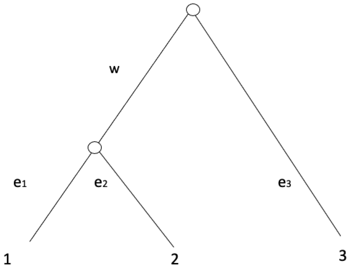
Phylogenomics is a new field, which applies tools from phylogenetics to genome data. In phylogenomics, we often conduct the species tree and gene trees analyses using the multi-species coalescent model [4]. Under the multi-species coalescent model, we assume that all gene trees, phylogenetic trees reconstructed from genes, are equidistant trees [4]. An equidistant tree is a rooted tree whose total branch length, from its root to each leaf, is the same for all leaves (an example of an equidistant tree with three leaves is shown in Figure 1).

In the past five years, there has been much work on the space of all equidistant trees for phylogenomics [5,6,7,8,9,10,11]. However, these recent studies assume that all given equidistant trees are true trees or close to true trees, which is often not true. Davidson and Sullivant worked on variability of a distance-based method to reconstruct an equidistant tree from all pairwise distances, called the Unweighted Pair Group Method with Arithmetic Mean (UPGMA) using polyhedral geometry [12]. They study how UPGMA project a given distance matrix to the space of all equidistant trees so that their result is from the view of polyhedral geometry and deterministic.

In this paper, therefore, we focus on the stochastic safety radius of the Unweighted Pair Group Method with Arithmetic Mean (UPGMA), one of the most popular distance-based methods and a lower bound of its probability that the UPGMA method returns the true tree topology from a random input distance matrix with noise distributed from the Gaussian distribution. Note that UPGMA is a hierarchical clustering method that builds a dendrogram from a distance matrix which records pairwise “distances” defined by a user input metric between all pairs of observations in a higher dimensional vector space [13]. In the application to a phylogenetic tree reconstruction, we use a distance matrix which contains pairwise distances between all pairs of sequences in the input alignment via a user input evolutionary model [1].

A phylogenetic tree is a weighted tree with labeled external nodes, called leaves, and unlabeled internal nodes. These labels represent species or taxa at the present time and each internal node represents a common ancestor for all of the leaves below this internal node. A weight on each branch (or edge) of a phylogenetic tree represents a mutation rate combined with its evolutionary time from an ancestor to its descendent. A phylogenic tree can be rooted or unrooted. For more details, see [1].

Example 1. 

Suppose we have a label set for leaves $X=\{1,2,3\}$ which represents a set of species at the present time. Suppose we have a rooted phylogenetic tree T shown in Figure 1.

Internal nodes on T do not have labels. The internal node of the ancestor of leaves $1,2$ represents the most common ancestral species of species $1,2$ and the root of T is the most common ancestor of all species $1,2,3$. Each branch length on a branch represents the mutation rate combined with its evolutionary time. A distance matrix computed from this tree shown in Figure 1 is a $3\times 3$ matrix such that $d_{ij}$, the $(i,j)$th cell of the matrix d is the total branch length from a leaf $i\in X$ to a leaf $j\in X$, that is,    

$$d=\begin{array}{|cccc|}\hline & 1& 2& 3\\ 1& 0& e_1+e_2& e_1+w+e_3\\ 2& e_1+e_2& 0& e_2+w+e_3\\ 3& e_1+w+e_3& e_2+w+e_3& 0\\ \hline\end{array}.$$

Since d is computed from a phylogenetic tree, d is a tree metric. Not all $n\times n$ symmetric matrices with diagonal elements equal to 0 are not tree metrics.

Through this paper, we assume that binary phylogenetic trees and the smallest branch length $w_{min}$ of an internal edge in a binary phylogenetic tree are strictly positive. In this paper, we focus on equidistant trees which are rooted phylogenetic trees with branch lengths such that the total branch length from its root to each leaf is the same.

Example 2. 

We consider a rooted phylogenetic tree on the label set of leaves $X=\{1,2,3\}$ shown in Figure 1 with $w>0$. If $w+e_1=w+e_2=e_3$, then T is an equidistant tree.

In this paper, our main contribution is that we show a lower bound of the probability of UPGMA to return the true equidistant tree on the set of leaves $X=\{1,2,\dots ,n\}$ for $n\ge 3$ from a set of random pairwise distances of all possible pairs of sequences. Then we conduct some computational experiments using a statistical software R to see how tight this lower bound is in practice for $n=4,\dots ,10$.

This paper is organized as follows: Section 2 reminds the reader of the basics of tree metrics and random variables representing pairwise distances of all possible pairs of sequences. Then it adds a notion of stochastic safety radius defined by Steel and Gascuel in [2]. In Section 3, we compute the stochastic safety radius of the three point condition for equidistant trees using a lower bound of the probability of returning the tree topology based on the three point condition. Then in Section 4, we compute a lower bound of the the probability of returning the tree topology from UPGMA and in Section 5, we show some results from our computational experiments with R. In Section 6, we end this paper with some discussion.

2. Stochastic Safety Radius

Let ${\mathbb{Z}}_{\ge 0}$ be the set of all non-negative integers. Let $X=\{1,\dots ,n\}$ be the set of labels for given species (or taxa) and let T be a rooted phylogenetic tree with leaves X.

Definition 3. 

Let $D\in {\mathbb{Z}}_{\ge 0}^{n\times n}$ be an $n\times n$ matrix with non-negative elements. If D is a symmetric matrix with its diagonal equal to 0, then we call D a distance matrix or dissimilarity maps.

Let $d_{ij}\in {\mathbb{Z}}_{\ge 0}$ be the $(i,j)$th element of a distance matrix D. If $d_{ij}$ satisfies

• $d_{ij}=d_{ji}$ for any $i,j\in X$,
• $d_{ii}=0$ for all $i\in X$,
• $d_{ik}+d_{kj}\ge d_{ij}$ for all $i,j,k\in X$,

then we call D ametric.

If D is a metric and if there exist a phylogenetic tree with leaves X such that $d_{ij}$ is the total distance of branch lengths of the path from a leaf i to a leaf j for all $i,j\in X$, then D is called a tree metric.

Suppose D is a metric on X. Then if D satisfies

$$\begin{array}{c}\hfill max\{d_{ij},d_{ik},d_{jk}\}\mathit{and}\mathit{is}\mathit{achieved}\mathit{at}\mathit{least}\mathit{twice},\end{array}$$

(1)

for distinct $i,j,k\in X$, then D is called an ultrametric.

Definition 4. 

Suppose we have a rooted phylogenetic tree T with a leaf label set X. If a distance from its root to each leaf $i\in X$ is the same distance for all $i\in X$, then we call T an equidistant tree.

Theorem 5 

([14]). Suppose we have an equidistant tree T with a leaf label set X and suppose $d_{ij}$ for all $i,j\in X$ is a distance from a leaf i to a leaf j. Then, D is an ultrametric if and only if T is an equidistant tree.

In this paper, we focus on equidistant trees with leaves X. In practice, we compute a distance matrix from an observed alignment. When we compute a distance matrix from an alignment via a maximum likelihood estimation, usually a distance matrix is not a tree metric [1]. Therefore, in this paper, we investigate a probability that we obtain the tree topology of the true phylogenetic tree from a distance matrix obtained from an input alignment using stochastic safety radius [2].

Definition 6 

(Stochastic safety radius). Let $\sigma =\frac{c^2}{log\left(n\right)}$ for some positive $c\in \mathbb{R}$. For any $\eta >0$, we say that a distance-based tree reconstruction method M has $\eta$-stochastic safety radius$s=s_n$ if for every binary phylogenetic X-tree T on n leaves, with minimum interior edge length $w_{min}>0$, and with the distance matrix δ on X described by the random errors model, we have

$$c<s·w_{min}\Rightarrow P(M\left(\delta \right)=T)\ge 1-\eta .$$

In this paper, we focus on the stochastic safety radius of a distance-based method, Unweighted Pair Group Method with Arithmetic Mean (UPGMA).

In reality, if we obtain all pairwise distances from a genetic data set, then we rarely have an ultrametric. Instead, we usually have dissimilarity maps. In order to infer an equidistant tree from dissimilarity maps, we can use UPGMA [15], which is a weighted least squared method to estimate the closest ultrametric in the space of ultrametrics [16].

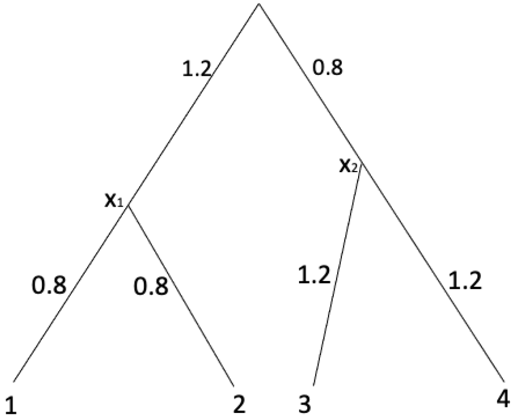
Example 7. 

In order to demonstrate Algorithm 1, consider an equidistant tree with $X=\{1,2,3,4\}$ shown in Figure 2.

Algorithm 1 UPGMA [15]

Input: Dissimilarity map $D\in {\mathbb{R}}^e$ on X. Output: An estimated equidistant tree T on X. Set $S:=X$ and $T=\varnothing$. for$k=1,\dots ,n-1$,  do     Pick smallest $D_{ij}$ for all pair of $(i,j)\in S$ with $i\ne j$. Set x as a parent node for the node i and j, compute branch length from i to x and j to x, and then record them in a tree T.     Set a new node x with $D_{xk}=\frac{1}{2}(D_{ik}+D_{jk})$ for all $k\in X$ with $k\ne i$ and $k\ne j$.     Remove $i,j$ from S and add x to S. end for Record the branch lengths from the root to each leaf in the two leaves. returnT.

Figure 2. Example for Algorithm 1.

Figure 2. Example for Algorithm 1.

A distance matrix computed from the tree shown in Figure 2 is

$$d=\begin{array}{|ccccc|}\hline \multicolumn{1}{c}{}& 1& 2& 3& 4\\ 1& 0& 1.6& 4& 4\\ 2& 1.6& 0& 4& 4\\ 3& 4& 4& 0& 2.4\\ 4& 4& 4& 2.4& 0\\ \hline\end{array}.$$

Note that

• For $i=1,j=2,k=3$:

  $$max\{d_{12},d_{13},d_{23}\}=4$$
  and

  $$d_{13}=d_{23}=4.$$
• $i=1,j=2,k=4$:

  $$max\{d_{12},d_{14},d_{24}\}=4$$
  and

  $$d_{14}=d_{24}=4.$$
• $i=1,j=3,k=4$:

  $$max\{d_{13},d_{14},d_{34}\}=4$$
  and

  $$d_{13}=d_{14}=4.$$
• $i=2,j=3,k=4$:

  $$max\{d_{23},d_{24},d_{34}\}=4$$
  and

  $$d_{23}=d_{24}=4.$$

Therefore, d satisfies Equation (3). Thus, this $4\times 4$ matrix is an ultrametric.

With UPGMA algorithm shown in Algorithm 1, we have

• For $k=1$, we pick a pair of leaves $(1,2)$ with $d_{12}=1.6$. Set $x_1$ as the parent node of $(1,2)$. Assign the branch length from $x_1$ to 1 as $1.6/2=0.8$ and assign the branch length from $x_1$ to 2 as $1.6/2=0.8$. Now we add $x=(1,2)$ as a leaf set X. Thus we have $X=\{x,3,4\}$ with

  $$d_{x3}=\frac{1}{2}(d_{13}+d_{23})=\frac{1}{2}(4+4)=4$$
  and

  $$d_{x4}=\frac{1}{2}(d_{14}+d_{24})=\frac{1}{2}(4+4)=4.$$
• For $k=2$, we pick a pair of leaves $(3,4)$ with $d_{34}=2.4$. Set $x_2$ as the parent node of $(3,4)$. Assign the branch length from $x_2$ to 3 as $2.4/2=1.2$ and assign the branch length from $x_2$ to 4 as $2.4/2=1.2$. Now we add $y=(3,4)$ as a leaf set y. Thus we have $X=\{x,y\}$ with

  $$d_{xy}=\frac{1}{2}(d_{x3}+d_{x4})=\frac{1}{2}(4+4)=4.$$

After the for-loop, we record the branch length from the root to the leaf x and the leaf y as $4/2=2$. From this, we can compute the branch length from the root to $x_1$ by $2-0.8=1.2$ and the branch length from the root to $x_2$ by $2-1.2=0.8$.

In this paper, we use UPGMA in order to investigate their stochastic safety radius and lower bounds for the probability for UPGMA to return the true tree topology if the input distance matrix is not ultrametric. Here we assume that the multivariate random variable $\delta$ is defined as follows:

$$\begin{array}{c}\hfill {\delta }_{ij}=d_{ij}+{ϵ}_{ij}\end{array}$$

(2)

where ${ϵ}_{ij}\sim N(0,\sigma )$ are independently and identically distributed for fixed $\sigma >0$ and for all $i<j\in X$ and

$${\delta }_{ji}={\delta }_{ij}$$

for all $i<j\in X$.

Remark 8. 

In order to make it simple, we assume that the height of an equidistant tree T on leaves X, which is the total branch length from each leaf $i\in X$ to its root, is equal to 1.

3. Probability on the Three Point Condition

From Equation (1), we have the three point condition which is defined below: for all distinct leaves $i,j,k\in X$ we have

$$\begin{array}{ccc}\hfill d_{ij}& \le & d_{ik}\hfill \\ \hfill d_{ij}& \le & d_{jk}\hfill \end{array}$$

(3)

and, by Theorem 5, if d is an ultrametric and is a tree metric of an equidistant tree T, then Equation (3) satisfies for all distinct leaves $i,j,k\in X$.

Suppose a subtree of T is a tree shown in Figure 3. Then we have the following:

$$\begin{array}{ccc}\hfill d_{ij}& =& e_i+e_j,\hfill \\ \hfill d_{ik}& =& e_i+e_k+w,\hfill \\ \hfill d_{jk}& =& e_j+e_k+w.\hfill \end{array}$$

(4)

In addition, from Equation (4), we have

$$\begin{array}{ccc}\hfill {\delta }_{ij}& =& e_i+e_j+{ϵ}_{ij},\hfill \\ \hfill {\delta }_{ik}& =& e_i+e_k+w+{ϵ}_{ik},\hfill \\ \hfill {\delta }_{jk}& =& e_j+e_k+w+{ϵ}_{jk}.\hfill \end{array}$$

(5)

Therefore, by Equation (5) and Equation (4), we have the following: for all distinct leaves $i,j,k\in X$ we have

$$\begin{array}{ccc}\hfill e_i+e_j+{ϵ}_{ij}& \le & e_i+e_k+w+{ϵ}_{ik}\hfill \\ \hfill e_i+e_j+{ϵ}_{ij}& \le & e_j+e_k+w+{ϵ}_{jk}.\hfill \end{array}$$

(6)

Then we have

$$\begin{array}{ccc}\hfill e_j+w+{ϵ}_{ij}& \le & e_k+2w+{ϵ}_{ik}\hfill \\ \hfill e_i+w+{ϵ}_{ij}& \le & e_k+2w+{ϵ}_{jk}.\hfill \end{array}$$

(7)

Since $e_i+w=w_k$ and $e_j+w=w_k$, we have

$$\begin{array}{ccc}\hfill {ϵ}_{ij}& \le & 2w+{ϵ}_{ik}\hfill \\ \hfill {ϵ}_{ij}& \le & 2w+{ϵ}_{jk}.\hfill \end{array}$$

(8)

Therefore, we have

$$\begin{array}{ccc}\hfill {ϵ}_{ij}-{ϵ}_{ik}& \le & 2w\hfill \\ \hfill {ϵ}_{ij}-{ϵ}_{jk}& \le & 2w.\hfill \end{array}$$

(9)

Since ${ϵ}_{ij},{ϵ}_{ik},{ϵ}_{jk}$ are independently and identically distributed (i.i.d.) from the normal distribution $N(0,\sigma )$, ${ϵ}_{ij}-{ϵ}_{ik}$ and ${ϵ}_{ij}-{ϵ}_{jk}$ are i.i.d. from the normal distribution $N(0,2\sigma )$. Therefore, we have

$$\begin{array}{ccc}& P(min\{{ϵ}_{ij}-{ϵ}_{ik}\}\le 2w)& \mathrm{for}\mathrm{all}i,j,k\in X\hfill \\ \hfill =& 1-P(min\{{ϵ}_{ij}-{ϵ}_{ik}\}>2w)& \mathrm{for}\mathrm{all}i,j,k\in X\hfill \\ \hfill =& 1-P(\frac{min\{{ϵ}_{ij}-{ϵ}_{ik}\}}{2}>w)& \mathrm{for}\mathrm{all}i,j,k\in X\hfill \\ \hfill =& 1-P{(\frac{{ϵ}^{\prime }}{2}>w)}^{\left(\genfrac{}{}{0pt}{}{n}{3}\right)}& \mathrm{where}{ϵ}^{\prime }\sim N(0,2\sigma )\hfill \\ \hfill =& 1-P{(ϵ>w)}^{\left(\genfrac{}{}{0pt}{}{n}{3}\right)}& \mathrm{where}ϵ\sim N(0,\sigma )\hfill \\ \hfill =& 1-P{(\frac{ϵ}{w}>1)}^{\left(\genfrac{}{}{0pt}{}{n}{3}\right)}& \mathrm{where}ϵ\sim N(0,\sigma )\hfill \\ \hfill =& 1-P{(ϵ>1)}^{\left(\genfrac{}{}{0pt}{}{n}{3}\right)}& \mathrm{where}ϵ\sim N\left(0,\frac{\sigma }{w}\right).\hfill \end{array}$$

(10)

Let $w=w_{min}$ where $w_{min}$ is the smallest branch length for an internal edge in an equidistant tree T on leaves X. Then we have

$$P(M\left(\delta \right)=T)\ge 1-P{(ϵ>1)}^{\left(\genfrac{}{}{0pt}{}{n}{3}\right)},$$

where $ϵ\sim N(0,\frac{\sigma }{w_{min}})$. Let $\sigma =\frac{c^2}{log\left(n\right)}$ for $c>0$ and $\eta =P{(ϵ>1)}^{\left(\genfrac{}{}{0pt}{}{n}{3}\right)}$. Let $c=s·w_{min}$. Then we have

$$\left(\frac{\sigma }{w_{min}}\right)=\left(\frac{s^2·w_{min}}{log\left(n\right)}\right)<\left(\frac{s^2}{log\left(n\right)}\right)$$

by Remark 8.

4. Probability Distribution of the Output Tree via Upgma

4.1. Case for $n=3$

For $n=3$, we have $X=\{1,2,3\}$. Suppose $d_{12}<d_{13}$ and $d_{12}<d_{23}$. from Equation (9), we have

$$\begin{array}{c}\hfill P(min\{{ϵ}_{12}-{ϵ}_{13}\}\le 2w)=1-P(ϵ>1)\hspace{1em}\mathrm{w}\mathrm{h}\mathrm{e}\mathrm{r}\mathrm{e} ϵ\sim N\left(0,\frac{\sigma }{w}\right).\end{array}$$

(11)

4.2. Case for $n=4$

For $n=4$, we have $X=\{1,2,3,4\}$.

Case 1

If we have a case in the left picture in Figure 4 for $i=1,j=2,k=3,l=4$. The probability that ${\delta }_{12}$ is chosen first is

$$\begin{array}{c}\hfill 1-P(ϵ>1)\hspace{1em}\mathrm{where} ϵ\sim N\left(0,\frac{\sigma }{w_{min}}\right).\end{array}$$

(12)

let x be the new label merging leaves $1,2$. Then

$$\begin{array}{c}{\delta }_{3x}=d_{13}+ϵ\hfill \\ {\delta }_{4x}=d_{14}+ϵ\hspace{1em}\mathrm{where} ϵ\sim N(0,\sigma ).\hfill \end{array}$$

(13)

Then the probability that ${\delta }_{x3}$ is chosen is

$$\begin{array}{c}\hfill 1-P(ϵ>1)\hspace{1em}\mathrm{where} ϵ\sim N\left(0,\frac{\sigma }{w_{min}}\right).\end{array}$$

(14)

Therefore, the probability that UPGMA returns the true tree topology is

$${\left(1-P(ϵ>1)\right)}^2$$

where $ϵ\sim N\left(0,\frac{\sigma }{w_{min}}\right)$.

Case 2

If we have a case in the right picture in Figure 4 for $i=1,j=2,k=3,l=4$. The probability that ${\delta }_{12}$ is chosen first is

$$\begin{array}{c}\hfill 1-P(ϵ>1)\hspace{1em}\mathrm{where} ϵ\sim N\left(0,\frac{\sigma }{w_{min}}\right).\end{array}$$

(15)

let x be the new label merging leaves $1,2$. Then

$$\begin{array}{c}{\delta }_{3x}=d_{13}+ϵ\hfill \\ {\delta }_{4x}=d_{14}+ϵ\hspace{1em}\mathrm{where} ϵ\sim N(0,\sigma ).\hfill \end{array}$$

(16)

Then the probability that ${\delta }_{34}$ is chosen is

$$\begin{array}{c}\hfill 1-P(ϵ>1)\hspace{1em}\mathrm{where} ϵ\sim N\left(0,\frac{\sigma }{w_{min}}\right).\end{array}$$

(17)

Therefore, the probability that UPGMA returns the true tree topology is

$${\left(1-P(ϵ>1)\right)}^2$$

where $ϵ\sim N\left(0,\frac{\sigma }{w_{min}}\right)$.

Remark 9. 

For $X=\{1,\dots ,n\}$, there are $(2n-3)!!=1·3·5\dots ·(2n-3)$ many different tree topologies of rooted phylogenetic trees on leaves X [1].

By Remark 9, there are $(2·4-3)!!=1·3·5=15$. Thus, we have the probability that UPGMA returns the tree topology is

$$15{\left(1-P(ϵ>1)\right)}^2$$

where $ϵ\sim N\left(0,\frac{\sigma }{w_{min}}\right)$.

4.3. General Case

For $n\ge 3$, we have $X=\{1,\dots ,n\}$. Using the same way with the case on $n=4$, by recursive computations and by Remark 9, we can obtain the probability of UPGMA to return the true tree topology is

$$(2n-3)!!{\left(1-P(ϵ>1)\right)}^{(n-2)}$$

where $ϵ\sim N\left(0,\frac{\sigma }{w_{min}}\right)$.

Theorem 10. 

Suppose we have a distance matrix δ defined by Equation (2) with a tree metric associated with the binary true phylogenetic tree T on the set of leaves $X=\{1,\dots ,n\}$ with the smallest internal branch length $w_{min}>0$. Then the probability for UPGMA to return the true tree topology on X is bounded by

$$(2n-3)!!{\left(1-P(ϵ>1)\right)}^{(n-2)}$$

where $ϵ\sim N\left(0,\frac{\sigma }{w_{min}}\right)$.

Proof. 

For $n=3$, it is trivial. For $n>3$, then suppose the statement holds for $n-1$. Then we want to show that the statement holds for n. First, we fix the tree topology. Let $i,j,k$ be subsets of $X=\{1,\dots ,n\}$ and form a partition on X. Then suppose $d_{ij}<d_{ik}$ and $d_{ij}<d_{jk}$. from Equation (9), we have

$$\begin{array}{c}\hfill P(min\{{ϵ}_{ij}-{ϵ}_{ik}\}\le 2w)=1-P(ϵ>1)\hspace{1em}\mathrm{where} ϵ\sim N\left(0,\frac{\sigma }{w}\right).\end{array}$$

(18)

Since we assume that the statement holds for $n-1$, for this particular tree topology, we have that the probability for UPGMA to return the true tree topology on X is bounded by

$${\left(1-P(ϵ>1)\right)}^{(n-2)}$$

where $ϵ\sim N\left(0,\frac{\sigma }{w_{min}}\right)$. Since there are $(2n-3)!!$ many tree topologies for n, we have the result.    □

5. Computational Experiments

In this computational experiment, we use the ape [17] and the phangorn packages [18,19] R packages for phylogenetic tree data structures, generating random trees, and UPGMA.

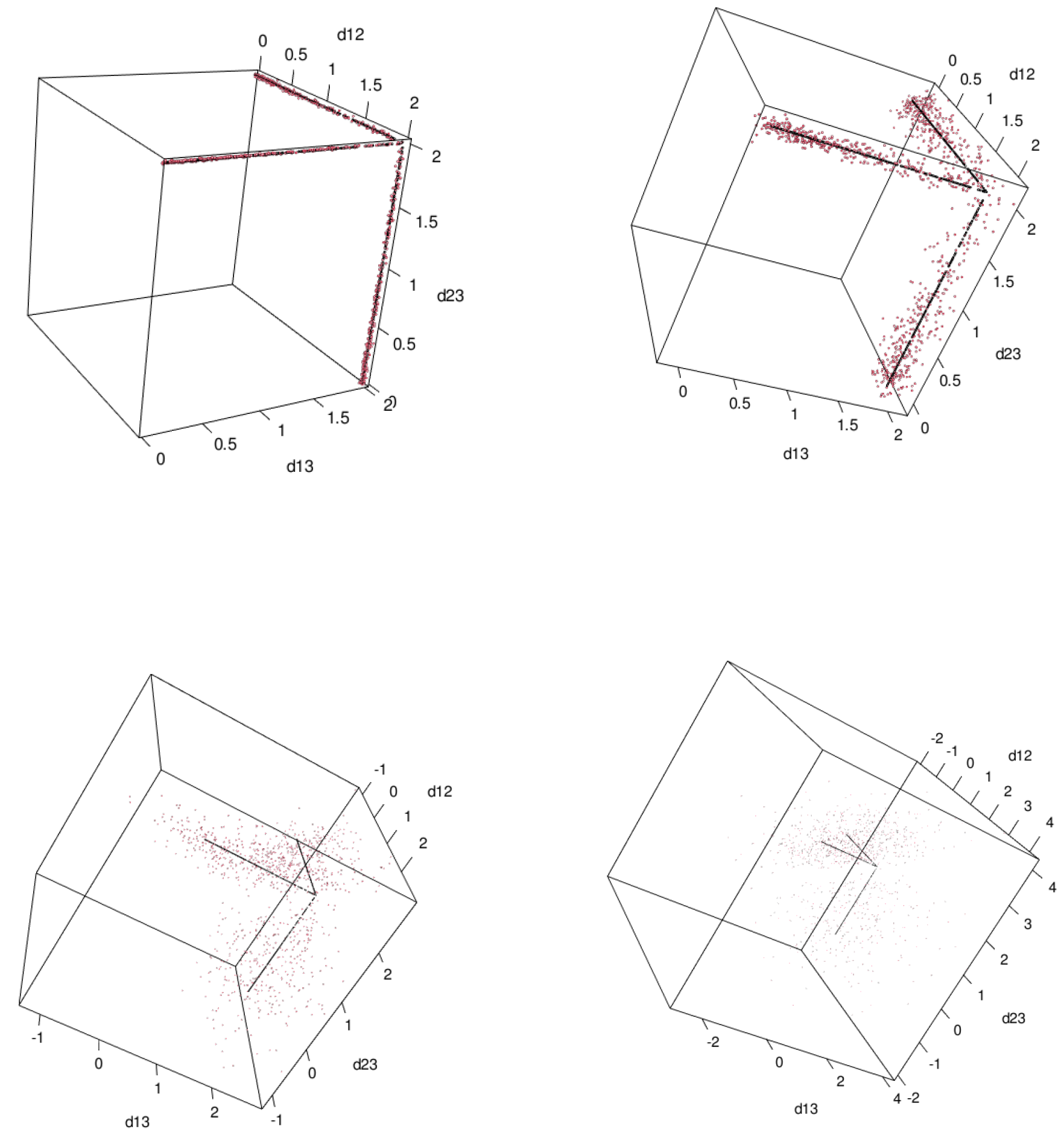
First, in order to compare Theorem 10 and the space of ultrametrics, namely Theorem 5 computationally with $n=3$ so that we can visualize the results. We generated 1000 random points $\delta =({\delta }_{12},{\delta }_{13},{\delta }_{23})$ where ${\delta }_{ij}=d_{ij}+ϵ$ for $i,j,k\in \{1,2,3\}$ and $ϵ\sim N(0,\sigma )$. We vary $\sigma =0.01,0.1,0.5,1.0$. The results show in Figure 5. Black points are ultrametrics $d=(d_{12},d_{13},d_{23})$ and red points are $\delta =({\delta }_{12},{\delta }_{13},{\delta }_{23})$.

We estimate the probability for UPGMA to return the true tree topology using Algorithm 2 for $n=4,\dots ,10$ and for $\sigma =0.1,0.5,1,2,5$, and then we compare these estimated probabilities with lower bounds which we obtained in Theorem 10. These results are shown in

Table 1. Comparison between empirical probabilities with lower bounds computed by Theorem 10. The notation $a\left(b\right)$ in each cell represents two parts: a represents the estimated probability for UPGMA to return the true tree topology with a random sample of sample size 1000 and (b) represents a lower bound computed by Theorem 10. We repeated this process 100 time and take an average for computing estimated probabilities. For example, we consider the cell for $\sigma =0.1$ and $n=4$. In this cell, 0.902 is an estimated probability computed by Algorithm 2 and 0.334 is a lower bound from Theorem 10 with $n=4$ and $\sigma =0.1$.

$\sigma$/ n	4	5	6	7
0.1	0.902 (0.334)	0.802 (0.447)	0.682 (0.381)	0.545 (0.260)
0.5	0.650 (0.160)	0.420 (0.055)	0.246 (0.035)	0.144 (0.014)
1	0.446 (0.060)	0.214 (0.006)	0.093 (0.001)	0.049 (<0.0001)
2	0.261 (0.015)	0.080 (0.001)	0.027 (<0.0001)	0.007 (<0.0001)
5	0.129 (0.004)	0.031 (<0.0001)	0.007 (<0.0001)	0.001 (<0.0001)
$\sigma$/ n	8	9	10
0.1	0.477 (0.226)	0.357 (0.137)	0.320 (0.118)
0.5	0.084 (0.001)	0.046 (<0.0001)	0.019 (<0.0001)
1	0.021 (<0.0001)	0.009 (<0.0001)	0.003 (<0.0001)
2	0.002 (<0.0001)	0.001 (<0.0001)	<0.001 (<0.0001)
5	<0.001 (<0.0001)	<0.001 (<0.0001)	<0.001 (<0.0001)

and

Table 2. Differences estimated probabilities minus lower bounds in Theorem 10 computed in our computational experiments shown in Table 1.

$\mathit{\sigma }$/ n	4	5	6	7	8	9	10
0.1	0.568	0.355	0.302	0.286	0.251	0.220	0.203
0.5	0.491	0.365	0.211	0.130	0.082	0.046	0.019
1	0.386	0.208	0.092	0.048	0.020	<0.001	<0.001
2	0.246	0.079	0.027	0.007	0.002	<0.001	<0.001
5	0.125	0.031	0.007	0.001	<0.001	<0.001	<0.001

. These results show that lower bounds computed in Theorem 10 might not be tight. In all cases, the lower bound computed by Theorem 10 is an order of magnitude less than the estimated probability for UPGMA to return the true tree topology with a random sample. This suggests that although the presence of a lower bound defines a boundary for the likelihood of the having the true tree topology, it also presents a challenge in the magnitude of gap.

Algorithm 2: Computational experiments for estimating the probability for UPGMA to return the true tree topology

Input: The number of leaves n, standard deviation $\sigma >0$. Output: Estimated probability for UPGMA to return the true tree topology. for$i=0,\dots ,100$, do     Generate a random tree T with n leaves $X=\{1,\dots ,n\}$ using a multispecies coalescent model [4] via the function coal from the ape package.     Set $p_i=0$.     for $k=0,\dots ,1000$, do         Generate a random distance matrix with $${\delta }_{ij}=d_{ij}+{ϵ}_{ij},$$ where $d_{ij}$ is the total branch length from a leaf i to a leaf j in T and ${ϵ}_{ij}\sim N(0,\sigma )$ for all $i,j\in X$.         Use UPGMA to reconstruct a tree $\widehat{T}$ from $\delta$ via the function upgma from the phangorn package.         Compare tree topology between T and $\widehat{T}$ using the function all.equal in the ape package.         if T and $\widehat{T}$ have the same tree topology, then            $p=p+1$.         end if     end for     $p_i=p_i/1000$. end for return $p=\frac{{\sum }_{i=1}^{100}{p}_i}{100}$.

6. Conclusions

UPGMA is a hierarchical clustering method to reconstruct a phylogenetic tree from a distance matrix. In general, it is unlikely that a given distance matrix is a tree metric so that, in this paper, we focus on the case when an input distance matrix is written as a linear combination of the true tree metric and an error term which is generated from the Gaussian distribution around 0 with the standard deviation $\sigma >0$. In addition, we show a lower bound of the probability for UPGMA to return the true tree topology if we have an input distance matrix $\delta$ defined by Equation (2).

Then we conduct computational experiments so that our lower bounds are close to the empirical probabilities estimated from random samples shown in Table 1 and Table 2. These computational results suggest our lower bounds are not tight. Thus, for a future direction of this research, we have the following questions:

Problem 11. 

Can we compute tighter lower bounds for UPGMA to return the true tree topology from a distance matrix δ defined in Equation (2)? If our bounds are tight for some situations, what are the conditions that our lower bounds are tight?

In addition, using the idea of computing lower bounds of the probability, we might be able to compute a “confidence interval” of the estimated phylogenetic tree from a given distance matrix via UPGMA.

References

1. Semple, C.; Steel, M. Phylogenetics; Number 22 in Mathematics and Its Applications Series; Oxford University Press: Oxford, UK, 2003. [Google Scholar]
2. Gascuel, O.; Steel, M. A ‘Stochastic Safety Radius’ for Distance-Based Tree Reconstruction. Algorithmica 2016, 74, 1386–1403. [Google Scholar] [CrossRef] [Green Version]
3. Xi, J.; Xie, J.; Yoshida, R.; Forcey, S. Stochastic safety radius on Neighbor-Joining method and Balanced Minimal Evolution on small trees. arXiv 2015, arXiv:1507.08734. [Google Scholar]
4. Maddison, W.P.; Maddison, D. Mesquite: A Modular System for Evolutionary Analysis. Evolution 2009, 2, 72. [Google Scholar]
5. Yoshida, R.; Zhang, L.; Zhang, X. Tropical Principal Component Analysis and its Application to Phylogenetics. Bull. Math. Biol. 2019, 81, 568–597. [Google Scholar] [CrossRef] [PubMed] [Green Version]
6. Yoshida, R.; Takamori, M.; Matsumoto, H.; Miura, K. Tropical Support Vector Machines: Evaluations and Extension to Function Spaces. Neural Netw. 2023, 157, 77–89. [Google Scholar] [CrossRef]
7. Lin, B.; Sturmfels, B.; Tang, X.; Yoshida, R. Convexity in Tree Spaces. SIAM Discret. Math 2017, 3, 2015–2038. [Google Scholar] [CrossRef] [Green Version]
8. Page, R.; Yoshida, R.; Zhang, L. Tropical principal component analysis on the space of phylogenetic trees. Bioinformatics 2020, 36, 4590–4598. [Google Scholar] [CrossRef] [PubMed]
9. Yoshida, R.; Miura, K.; Barnhill, D.; Howe, D. Tropical Density Estimation of Phylogenetic Trees. arXiv 2022, arXiv:2206.04206. [Google Scholar]
10. Yoshida, R.; Cox, S. Tree Topologies along a Tropical Line Segment. Vietnam. J. Math. 2022, 50, 395–419. [Google Scholar] [CrossRef]
11. Monod, A.; Lin, B.; Yoshida, R. Tropical Geometric Variation of Tree Shapes. Discret. Comput. Geom. 2022, 68, 817–849. [Google Scholar]
12. Davidson, R.; Sullivant, S. Polyhedral combinatorics of UPGMA cones. Adv. Appl. Math. 2013, 50, 327–338. [Google Scholar] [CrossRef] [Green Version]
13. James, G.; Witten, D.; Hastie, T.; Tibshirani, R. An Introduction to Statistical Learning: With Applications in R; Springer: New York, NY, USA, 2013. [Google Scholar]
14. Buneman, P. A note on the metric properties of trees. J. Comb. Theory Ser. B. 1974, 17, 48–50. [Google Scholar] [CrossRef] [Green Version]
15. Sokal, R.R.; Michener, C.D. A statistical method for evaluating systematic relationships. Univ. Kans. Sci. Bull. 1958, 38, 1409–1438. [Google Scholar]
16. Bernstein, D.I.; Long, C. L-Infinity Optimization to Linear Spaces and Phylogenetic Trees. SIAM J. Discret. Math. 2017, 31, 875–889. [Google Scholar] [CrossRef] [Green Version]
17. Paradis, E.; Schliep, K. ape 5.0: An environment for modern phylogenetics and evolutionary analyses in R. Bioinformatics 2019, 35, 526–528. [Google Scholar] [CrossRef] [PubMed]
18. Schliep, K. Phangorn: Phylogenetic analysis in R. Bioinformatics 2011, 27, 592–593. [Google Scholar] [CrossRef] [PubMed] [Green Version]
19. Schliep, K.; Potts, A.A.; Morrison, D.A.; Grimm, G.W. Intertwining phylogenetic trees and networks. Methods Ecol. Evol. 2017, 8, 1212–1220. [Google Scholar] [CrossRef]
Figure 1. Example of a phylogenetic tree T on the label set of leaves X = { 1 , 2 , 3 } .
Algorithms 15 00483 g001
Figure 3. Equidistant tree with three leaves on labels X = { i , j , k } . w , e i , e j , e k > 0 are branch lengths.
Algorithms 15 00483 g003
Figure 4. Two cases for equidistant trees without labels.
Algorithms 15 00483 g004
Figure 5. Red points are randomly generated δ = ( δ 12 , δ 13 , δ 23 ) and black points are ultrametrics which are equivalent to equidistant trees. The top left figure is for σ = 0.01 . The top right figure is for σ = 0.1 . The bottom left figure is for σ = 0.5 . The bottom right figure is for σ = 1 .
Algorithms 15 00483 g005