NSGA-PINN: A Multi-Objective Optimization Method for Physics-Informed Neural Network Training

Abstract

This paper presents NSGA-PINN, a multi-objective optimization framework for the effective training of physics-informed neural networks (PINNs). The proposed framework uses the non-dominated sorting genetic algorithm (NSGA-II) to enable traditional stochastic gradient optimization algorithms (e.g., ADAM) to escape local minima effectively. Additionally, the NSGA-II algorithm enables satisfying the initial and boundary conditions encoded into the loss function during physics-informed training precisely. We demonstrate the effectiveness of our framework by applying NSGA-PINN to several ordinary and partial differential equation problems. In particular, we show that the proposed framework can handle challenging inverse problems with noisy data.

1. Introduction

Physics-informed neural networks (PINNs) [1,2] have proven to be successful in solving partial differential equations (PDEs) in various fields, including applied mathematics [3], physics [4], and engineering systems [5,6,7]. For example, PINNs have been utilized for solving Reynolds-averaged Navier–Stokes (RANS) simulations [8] and inverse problems related to three-dimensional wake flows, supersonic flows, and biomedical flows [9]. PINNs have been especially helpful in solving PDEs that contain significant nonlinearities, convection dominance, or shocks, which can be challenging to solve using traditional numerical methods [10]. The universal approximation capabilities of neural networks [11] have enabled PINNs to approach exact solutions and satisfy initial or boundary conditions of PDEs, leading to their success in solving PDE-based problems. Moreover, PINNs have successfully handled difficult inverse problems [12,13] by combining them with data (i.e., scattered measurements of the states).

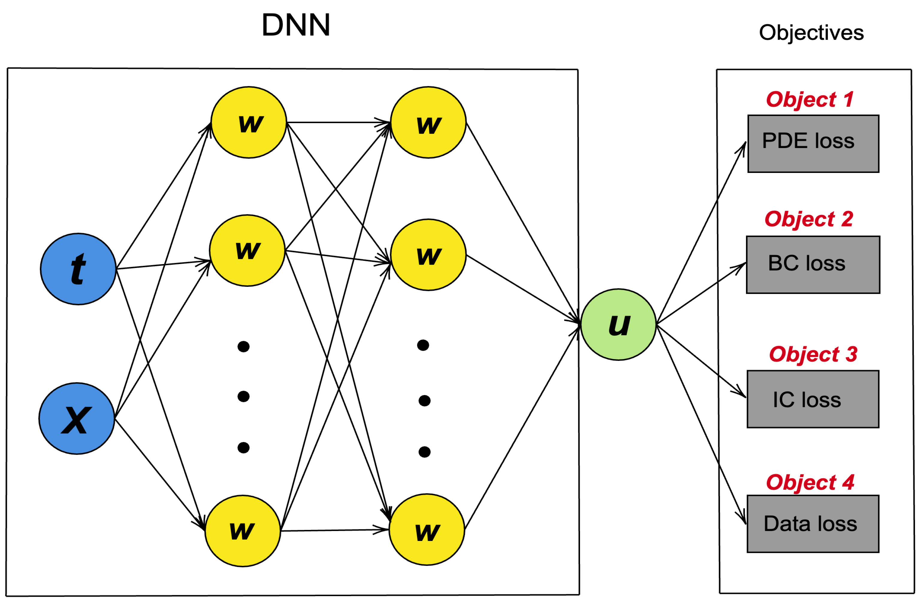
PINNs use multiple loss functions, including residual loss, initial loss, boundary loss, and, if necessary, data loss for inverse problems. The most common approach for training PINNs is to optimize the total loss (i.e., the weighted sum of the loss functions) using standard stochastic gradient descent (SGD) methods [14,15], such as ADAM. However, optimizing highly non-convex loss functions for PINN training with SGD methods can be challenging because there is a risk of being trapped in various suboptimal local minima, especially when solving inverse problems or dealing with noisy data [16,17]. Additionally, SGD can only satisfy initial and boundary conditions as soft constraints, which may limit the use of PINNs in the optimization and control of complex systems, which require the exact fulfillment of these constraints.

To meet the above constraints exactly, it may be helpful to use non-gradient methods, such as evolutionary algorithms (EAs) [18]. These methods are practical alternatives, particularly when gradient information is unavailable, or a large search space is necessary to ensure optimal convergence. Evolutionary algorithms typically rely on a population of candidate solutions that evolve over time through processes such as selection, mutation, and crossover. They have been applied successfully to a wide range of optimization problems, including constrained optimization [19], combinatorial optimization [20], multi-objective optimization [21] and neural network training [22].

In their paper [23], Rafael Bischof et al. suggest using multi-objective optimization techniques to train PINNs. They simplify the multi-objective into a single objective via linear scalarization and employ various methods to balance the different components of multi-objective optimization. In ref. [24], Bahador Bahmani et al. propose vectorizing each loss function in PINN and handling each pair of conflicting vectors by projecting one of the conflicting gradient vectors onto the normal plane of the other gradient vector. The projection is then used to adjust the descent direction during training. However, to the best of the authors’ knowledge, no prior research has focused on treating each element of the PINN loss function as a distinct objective and utilizing multi-objective techniques to minimize the loss in PINNs.

In this paper, we propose the NSGA-PINN framework, a multi-objective optimization method for PINN training. Specifically, we treat each part of the PINN loss as an objective and employ the non-dominated sorting algorithm II (NSGA-II) [21] and SGD methods to optimize these objectives. Our experimental results demonstrate that the proposed framework effectively helps in escaping the local minima and enables satisfying the system’s constraints, such as the initial and boundary conditions.

The rest of the paper is organized as follows. First, in Section 2, we provide a brief introduction to the following background information: PINN, SGD method, and NSGA-II algorithm. Then, in Section 3, we describe our proposed NSGA-PINN method. In Section 4, we present the experimental results using the inverse ODE problem and PDE problems to study the behavior of NSGA-PINN. We also test the robustness of our method in the presence of noisy data. Our results are discussed in Section 5. Finally, we conclude the paper in Section 6.

2. Background

In this section, we describe the physics-informed neural networks (PINNs) framework, the stochastic gradient descent (SGD) method, and non-dominated sorting algorithm-II (NSGA-II).

2.1. Physics-Informed Neural Networks

In our work, we consider computing data-driven solutions to partial differential equations (PDEs) of the general form

$$\begin{array}{c}\hfill u_t+\mathcal{N}[u:\lambda ]=0,x\in \mathsf{\Omega },t\in [0,T]\end{array}$$

(1)

Here, u represents the solution of the PDE, $\mathsf{\Omega }\subset {\mathbb{R}}^d$ represents the spatial domain, and $\mathcal{N}[:]$ denotes a differential operator.

The goal of PINN is to learn a parametric surrogate $u_{\theta }$ with trainable parameters $\theta$ that approximates the solution u. To achieve this goal, a neural network is constructed, and the total loss function of PINN is minimized. The total loss function consists of several components: residual loss, initial loss, boundary loss, and data loss, i.e,

$$\begin{array}{c}\hfill {\mathcal{L}}_{total}=w_f{\mathcal{L}}_{res}+w_g{\mathcal{L}}_{ics}+w_j{\mathcal{L}}_{bc}+w_h{\mathcal{L}}_{data}.\end{array}$$

(2)

We use the coefficients w to balance the loss terms. Each loss term is calculated by applying the L2 approximation [25]. In particular, ${\mathcal{L}}_{res}$ denotes the residual loss, which is the difference between the exact value of the PDE and the predicted value from the PINN deep neural network (DNN):   

$$\begin{array}{c}\hfill {\mathcal{L}}_{res}=\frac{1}{N_r}\sum _{i=1}^{N_r}{\left||u_{\theta }\left(x_i^r\right)-u\left(x_i^r\right)|\right|}^2\end{array}$$

(3)

In the above, we only considered the problem in the spatial domain for the sake of simplicity. Extending it to the temporal domain is straightforward. Moreover, $u_{\theta }\left(x_i^r\right)$ represents the output value of the PINN DNN on a set of $N_r$ points sampled within the spatial domain $\mathsf{\Omega }$. This can be computed using automatic differentiation methods [26]. On the other hand, $u\left(x_i^r\right)$ denotes the true solution of the PDE.

The initial or boundary loss represents the difference between the true solution and the predicted value from the PINN DNN at the initial or boundary condition. For instance, the boundary loss (for a given boundary condition h) at a set of $N_b$ boundary points $x_i^b$ is defined as follows:

$$\begin{array}{c}\hfill {\mathcal{L}}_{bc}=\frac{1}{N_b}\sum _{i=1}^{N_b}{\left||u_{\theta }\left(x_i^b\right)-h\left(x_i^b\right)|\right|}^2\end{array}$$

(4)

Furthermore, if we tackle inverse problems and have a set of $N_d$ experimental data points $y_i^d$, we can calculate the data loss using the PDE equation as follows:

$$\begin{array}{c}\hfill {\mathcal{L}}_{data}=\frac{1}{N_d}\sum _{i=1}^{N_d}{\left||u_{\theta }\left(x_i^d\right)-y_i^d|\right|}^2\end{array}$$

(5)

As shown in Equation (2), the loss value of a physics-informed neural network (PINN) is calculated as a simple linear combination with soft constraints. In this paper, we consider each part of the loss as an objective as shown in Figure 1.

2.2. Stochastic Gradient Decent

Stochastic gradient descent (SGD) and its variants, such as ADAM, are the most commonly used optimization methods for training neural networks (NN). SGD uses mini-batches of data, which are subsets of data points randomly selected from the training dataset. This injects noise into the updates during neural network training, enabling the exploration of the non-convex loss landscape. The optimization problem for SGD can be written as follows:   

$$\begin{array}{c}\hfill {\theta }^{*}=\arg \underset{\theta }{min}\mathcal{L}(\theta ;\mathcal{T}).\end{array}$$

(6)

This paper focuses on a variant of SGD known as the adaptive moment estimates (ADAM) optimizer. ADAM is the most popular and fastest method used in deep learning. The optimizer requires only first-order gradients and has very little memory requirement. It results in effective neural network (NN) training and generalization.

However, applying SGD methods to PINN training presents inevitable challenges. For complex non-convex PINN loss functions, SGD methods can get stuck in a local minimum, particularly when solving inverse problems with PINNs or dealing with noisy data.

2.3. NSGA-II Algorithm

In our work, we employ the NSGA-II algorithm, renowned for its efficiency and elitism, to tackle multi-objective optimization problems with speed and accuracy. The NSGA-II is used to search for good solutions when the solutions is convinced to lie somewhere is a space of possible candidate solutions—the search space [27]. With the properties of a fast nondominated sorting procedure (requires $O\left(M{N}^2\right)$ computations), an elitist strategy to preserve the population density and a simple yet efficient constraint-handling method, we utilize NSGA-II to deal with multi-objective problem in PINN.

Like EAs, NSGA-II mainly consists of a parent population and genetic operators such as crossover, mutation, and selection parts. Additionally, to solve multi-objective problems, the NSGA-II algorithm uses non-dominated sorting to assign a front value to each solution and calculates the density of each solution in the population using crowding distance. It then uses crowded binary selection to choose the best solutions based on front value and density value. We use these functions in our NSGA-PINN method, and we will explain them in detail in Section 3.

3. The NSGA-PINN Framework

This section describes the proposed NSGA-PINN framework for multi-objective optimization-based training of a PINN.

3.1. Non-Dominated Sorting

The proposed NSGA-PINN utilizes non-dominated sorting (see Algorithm 1 for more detailed information) during PINN training. The input P can consist of multiple objective functions, or loss functions, depending on the problem setting. For a simple ODE problem, these objective functions may include a residual loss function, an initial loss function, and a data loss function (if experimental data are available and we are tackling an inverse problem). Similarly, for a PDE problem, the objective functions may include a residual loss function, a boundary loss function, and a data loss function.

In the EAs, the solutions refer to the elements in the parent population. We randomly choose two solutions in the parent population p and q; if p has a lower loss value than q in all the objective functions, we define p as dominating q. If p has at least one loss value lower than q, and all others are equal, the previous definition also applies. For each p element in the parent population, we calculate two entities: (1) domination count $n_p$, which represents the number of solutions that dominate solution p, and (2) $S_p$, the set of solutions that solution p dominates. Solutions with a domination count of $n_p=0$ are considered to be in the first front. We then look at $S_p$ and, for each solution in it, decrease their domination count by 1. The solutions with a domination count of 0 are considered to be in the second front. By performing the non-dominated sorting algorithm, we obtain the front value for each solution [21].

Algorithm 1: Non-dominated sorting

3.2. Crowding-Distance Calculation

In addition to achieving convergence to the Pareto-optimal set for multi-objective optimization problems, it is important for an evolutionary algorithm (EA) to maintain a diverse range of solutions within the obtained set. We implement the crowding-distance calculation method to estimate the density of each solution in the population. To do this, first, sort the population according to each objective function value in ascending order. Then, for each objective function, assign infinite distance values to the boundary solutions, and assign all other intermediate solutions a distance equal to the absolute normalized difference in function values between two adjacent solutions. The overall crowding-distance value is calculated as the sum of individual distance values corresponding to each objective. A higher density value represents a solution that is far away from other solutions in the population.

3.3. Crowded Binary Tournament Selection

The crowded binary tournament selection, explained in more detail in Algorithm 2, was used to select the best PINN models for the mating pool and further operations. Before implementing this selection method, we labeled each PINN model so that we could track the one with the lower loss value. The population of size n was then randomly divided into $n/2$ groups, each containing two elements. For each group, we compared the two elements based on their front and density values. We preferred the element with a lower front value and a higher density value. In Algorithm 2, F denotes the front value and D denotes the density value.

Algorithm 2: Crowded binary tournament selection

3.4. NSGA-PINN Main Loop

The main loop of the proposed NSGA-PINN method is described in Algorithm 3. The algorithm first initializes the number of PINNs to be used (N) and sets the maximum number of generations ($\alpha$) to terminate the algorithm. Then, the PINN pool is created with N PINNs. For each loss function in a PINN, N loss values are obtained from the network pool. When there are three loss functions in a PINN, $3N$ loss values are used as the parent population. 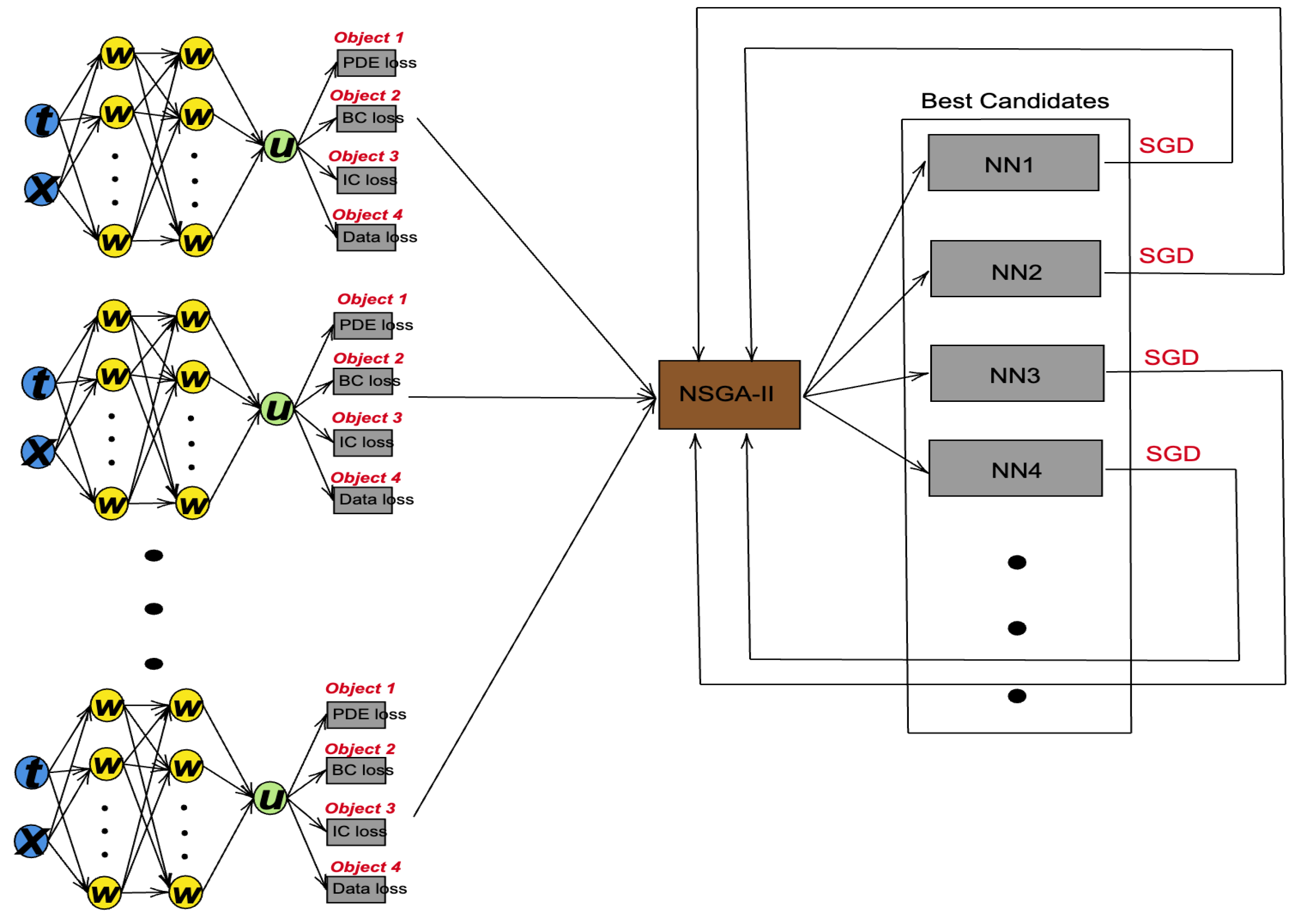The population is sorted based on non-domination, and each solution is assigned a fitness (or rank) equal to its non-domination level [21]. The density of each solution is estimated using crowding-distance sorting. Then, by performing a crowded binary tournament selection, PINNs with lower front values and higher density values are selected to be put into the mating pool. In the mating pool, the ADAM optimizer is used to further reduce the loss value. The NSGA-II algorithm selects the PINN with the lowest loss value as the starting point for the ADAM optimizer. By repeating this process many times, the proposed method helps the ADAM optimizer escape the local minima. Figure 2 shows the main process of the proposed NSGA-PINN framework.    

Algorithm 3: Training PINN by NSGA-PINN method

4. Numerical Experiments

This section evaluates the performance of physics-informed neural networks (PINN) trained with the proposed NSGA-PINN algorithm. We tested our framework on both the ordinary differential equation (ODE) and partial differential equation (PDE) problems. Our proposed method is implemented using the PyTorch library. For each problem, we compared the loss values of each component of the PINN trained with the NSGA-PINN algorithm to the loss values obtained from the PINN trained with the ADAM method, using the same neural network structure and hyperparameters. To test the robustness of the proposed NSGA-PINN algorithm, we added noise to the experimental data used in each inverse problem.

4.1. Inverse Pendulum Problem

The algorithm was first used to train PINN on the inverse pendulum problem without noise. The pendulum dynamics are described by the following initial value problem (IVP):

$$\begin{array}{cc}\hfill & \dot{\theta }\left(t\right)=\omega \left(t\right)\hfill \\ \hfill & \dot{\omega }\left(t\right)=-ksin\theta \left(t\right)\hfill \end{array}$$

(7)

where the initial condition is sampled as follows $(\theta \left(0\right),\omega \left(0\right))=({\theta }_0,{\omega }_0)\in [-\pi ,\pi ]\times [0,\pi ]$ and the true parameter unknown parameter $k=1.0$.

Our goal is to approximate the mapping using a surrogate physics-informed neural network: ${\theta }_0,{\omega }_0,t\mapsto \theta \left(t\right),\omega \left(t\right)$. For this example, we used a neural network for PINN consisting of 3 hidden layers and 100 neurons in each layer. The PINN training loss for the neural network is defined as follows:

$$\begin{array}{c}\hfill \mathcal{L}={\mathcal{L}}_{res}+{\mathcal{L}}_{ics}+{\mathcal{L}}_{data}.\end{array}$$

(8)

To determine the total loss in this problem, we add the residual loss, initial loss, and data loss. We calculate the data loss using the mesh data $t_s$, which ranges from 0 to 1 (seconds) with a step size of 0.01. We fit these data onto the ODE to determine the data loss value accurately. For this problem, we set the parent population to 20 and the maximum number of generations to 20 in our NSGA-PINN.

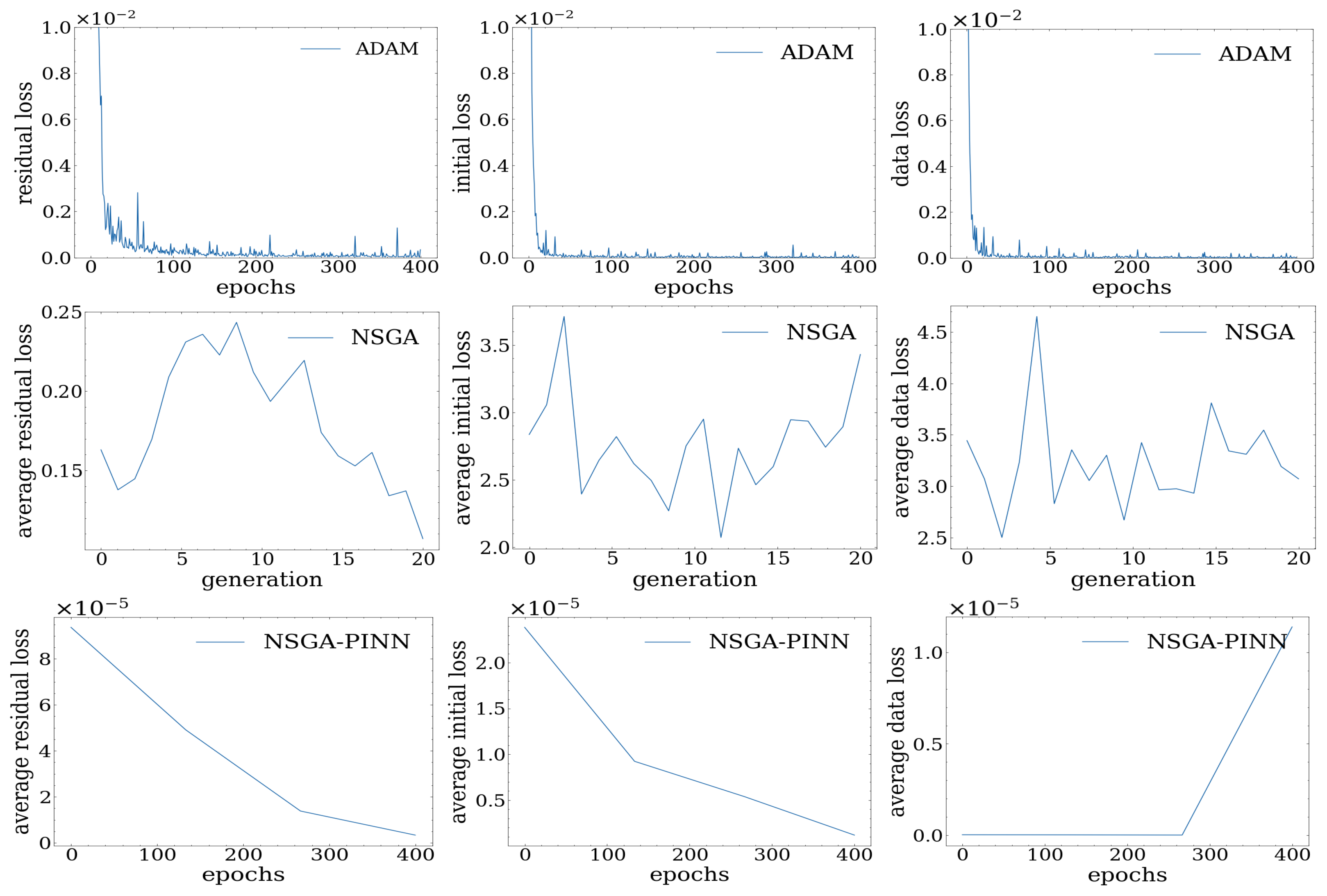
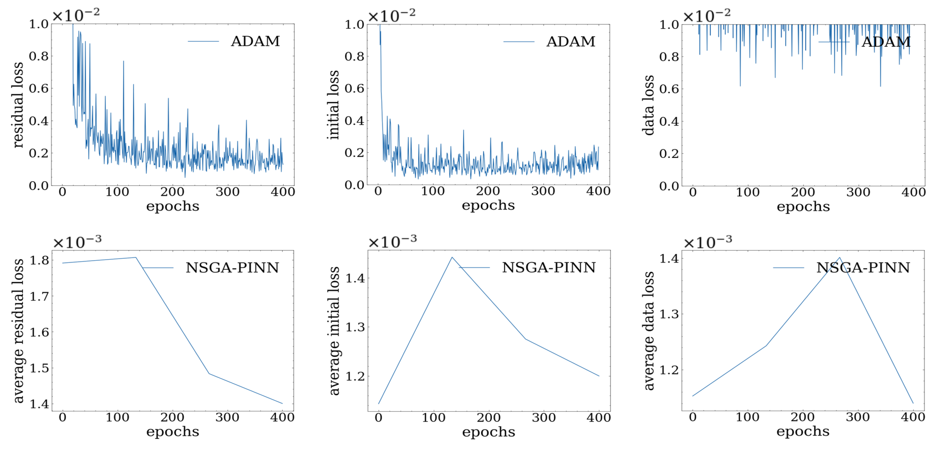
In the course of our experiment, we tested various methods, which are illustrated in Figure 3.

Based on our observations, we found that the ADAM optimizer did not yield better results after 400 epochs, as the loss value remained in the scale of $1\times {10}^{-2}$. We also tried the NSGA-II algorithm for PINN, which introduced some diversity to prevent the algorithm from getting stuck at local minima, but the loss value was still around 4.0. Ultimately, we implemented our proposed NSGA-PINN algorithm to train PINN on this problem, resulting in a significant improvement with a loss value to the scale of $1\times {10}^{-5}$.

To gain a clear understanding of the differences in loss values between optimization methods, we collected numerical loss values from our experiment. For the NSGA and NSGA-PINN methods, loss values were calculated as the average since they are obtained using ensemble methods through multiple runs. Our observations presented in

Table 1. Inverse pendulum problem: Each loss value from NN trained by using different training methods.

Methods	Residual Loss	Initial Loss	Data Loss	Total Loss
ADAM	0.00013	$3.24\times {10}^{-5}$	$3.11\times {10}^{-5}$	$1.935\times {10}^{-4}$
NSGA	0.12	2.67	4.10	6.89
NSGA-PINN	$3.94\times {10}^{-5}$	$1.21\times {10}^{-5}$	$1.41\times {10}^{-5}$	$6.55\times {10}^{-5}$

revealed that the total loss value of PINN trained with the traditional ADAM optimizer decreased to $1.935\times {10}^{-4}$. However, by training with the NSGA-PINN method, the loss value decreased even further to $6.55\times {10}^{-5}$, indicating improved satisfaction with the initial condition constraints.

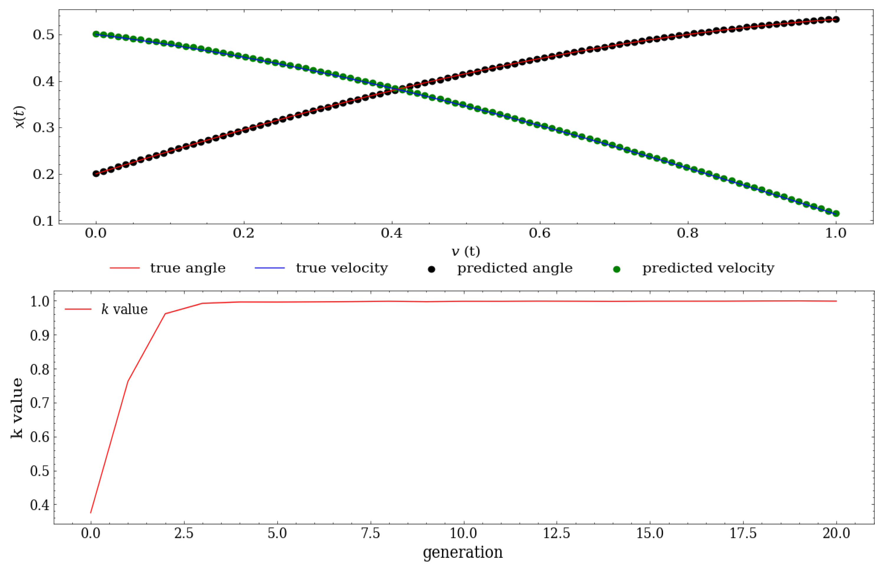
In Figure 4, we compare the predicted angle and velocity state values to the true values to analyze the behavior of the proposed NSGA-PINN method. The top figure shows how accurately the predicted values match the true values, illustrating the successful performance of our algorithm. At the bottom of the figure, we observe the predicted value of the parameter k, which agrees with the true value of $k=1$. This result was obtained after running our NSGA-PINN algorithm for three generations.

4.2. Inverse Pendulum Problem with Noisy Data

In this section, we introduce Gaussian noise to the experimental data collected for the inverse problem. The noise was sampled from the Gaussian distribution:

$$\begin{array}{c}\hfill P\left(x\right)=\frac{1}{\sigma \sqrt{2\pi }}{e}^{-{\left(x-\mu \right)}^2/\phantom{-{\left(x-\mu \right)}^{2}2{\sigma }^2}2{\sigma }^2}\end{array}$$

(9)

For this experiment, we chose to set the mean value ($\mu$) to 0 and the standard deviation of the noise ($\sigma$) to 0.1. As depicted in Figure 5, we trained the PINN model using the ADAM optimizer. However, we encountered an issue where the loss value failed to decrease after 400 epochs. This suggested that the optimizer had become stuck in a local minimum, which is a common problem associated with the ADAM optimizer when presented with noise.

To address this issue, we implemented the proposed NSGA-PINN method, resulting in significant improvements. Specifically, by increasing the diversity of the NSGA population, we were able to escape the local minimum and converge to a better local optimum, where the initial condition constraints were more effectively satisfied.

By examining

Table 2. Inverse pendulum problem with data noise: each loss value from NN trained by different training methods with noisy data.

Methods	Residual Loss	Initial Loss	Data Loss	Total Loss
ADAM	0.0028	0.0028	0.0114	0.017
NSGA-PINN	0.0010	0.0011	0.0112	0.0133

, we can see a clear numerical difference between the two methods. Specifically, the table shows that the PINN trained by the ADAM method has a total loss value of 0.017, while the PINN trained by the proposed NSGA-PINN method has a total loss value of 0.0133.

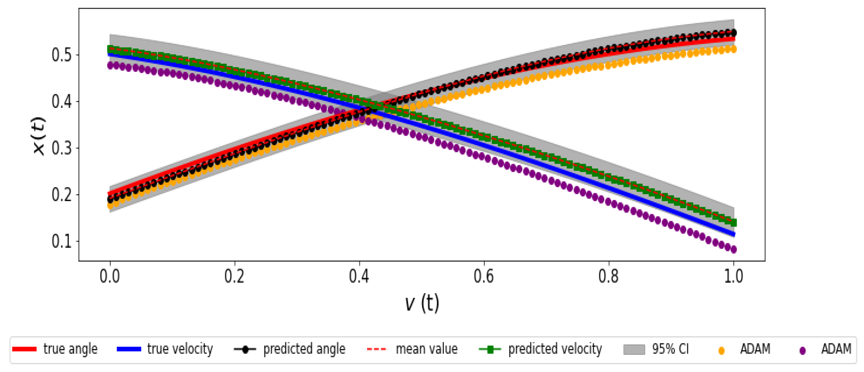
Finally, in Figure 6, we quantify uncertainty using an ensemble of predictions from our proposed method. This ensemble allows us to compute the 95% confidence interval, providing a visual estimate of the uncertainty. To calculate the mean value, we averaged the predicted solutions from an ensemble of 100 PINNs trained by the NSGA-PINN algorithm. Our observations indicate that the mean is close to the solution, demonstrating the effectiveness of the proposed method. When comparing the predicted trajectory from the PINN trained with the NSGA-PINN algorithm to the one trained with the ADAM method, we found that the NSGA-PINN algorithm yields results closer to the real solution in this noisy scenario.

4.3. Burgers Equation

This experiment uses the Burgers equation to study the effectiveness of the proposed NSGA-PINN algorithm on a PDE problem. The Burgers equation is defined as follows:

$$\begin{array}{cc}\hfill & \frac{du}{dt}+u\frac{du}{dx}=v\frac{d^{2}u}{d{x}^2},x\in [-1,1],t\in [0,1]\hfill \\ \hfill & u(0,x)=-sin\left(\pi x\right)\hfill \\ \hfill & u(t,-1)=u(t,1)=0\hfill \end{array}$$

(10)

Here, u is the PDE solution, $\mathsf{\Omega }=[-1,1]$ is the spatial domain, and $v=0.01/\pi$ is the diffusion coefficient.

The nonlinearity in the convection term causes the solution to become steep, due to the small value of the diffusion coefficient v. To address this problem, we utilized a neural network for PINN, which consisted of 8 hidden layers with 20 neurons each. The hyperbolic tangent activation function was used to activate the neurons in each layer. We sampled 100 data points on the boundaries and 10,000 collocation data points for PINN training.

For the proposed NSGA-PINN method, the original population size was set to 20 neural networks, and the algorithm ran for 20 generations. The loss function in the Burgers’ equation can be defined as follows:

$$\begin{array}{c}\hfill \mathcal{L}={\mathcal{L}}_u+{\mathcal{L}}_b+{\mathcal{L}}_{ics}.\end{array}$$

(11)

Here, the total loss value is the combination of the residual loss, the initial condition loss, and the boundary loss.

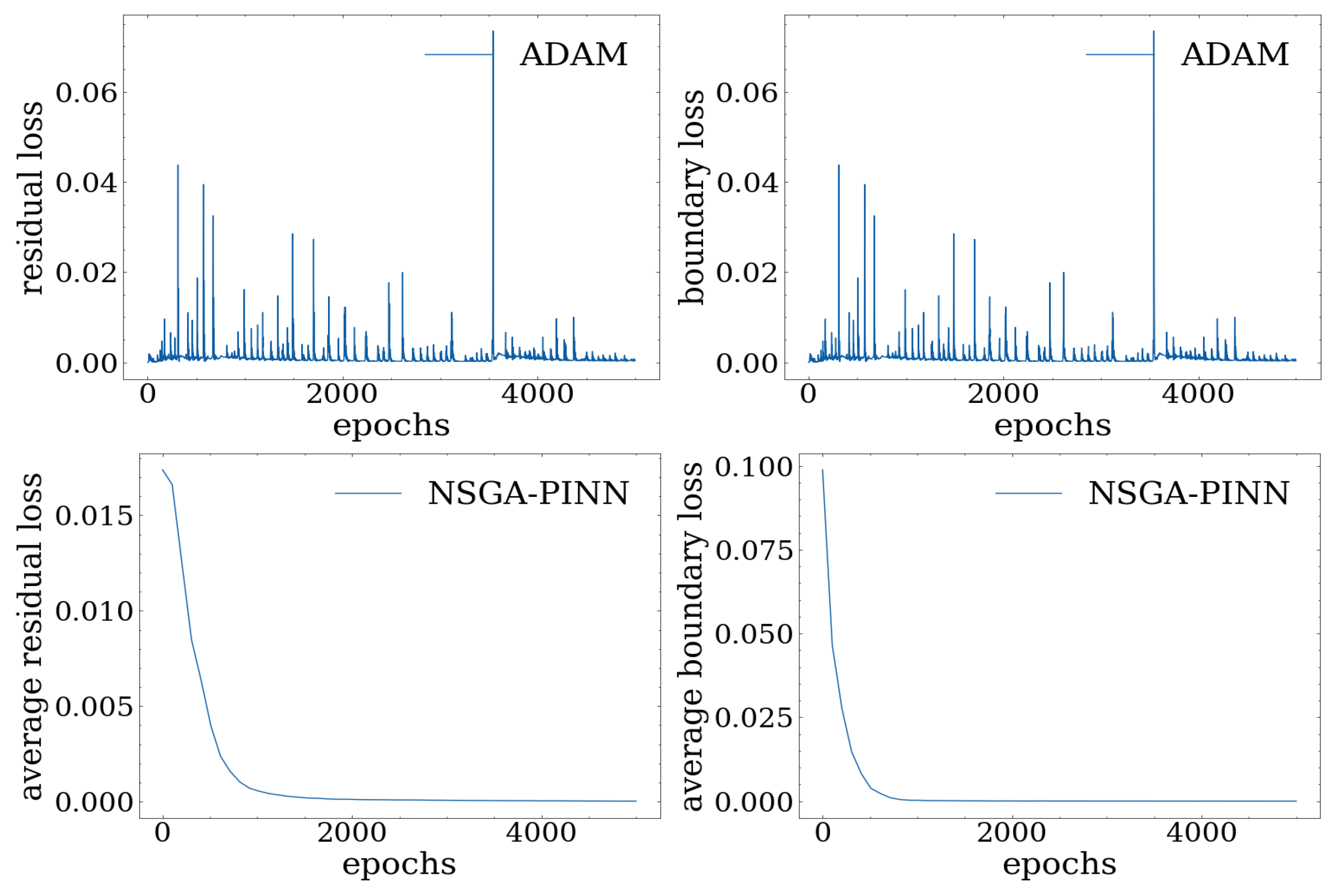
We can observe the effectiveness of the proposed NSGA-PINN algorithm by examining the loss values depicted in Figure 7 and

Table 3. Burgers equation: Comparison of the loss value from NN trained by ADAM method and NSGA-PINN method for Burgers equation.

Methods	Residual Loss	Boundary Loss	Total Loss
ADAM	0.0002	$9.4213\times {10}^{-5}$	0.0003
NSGA-PINN	$2.89\times {10}^{-5}$	$8.56\times {10}^{-6}$	$3.746\times {10}^{-5}$

. In particular, Table 3 compares the loss values of PINNs trained by the NSGA-PINN algorithm and the traditional ADAM method. Noticeably, the loss value trained by the NSGA-PINN framework is $3.746\times {10}^{-5}$, which is much lower than the traditional ADAM method, which has the loss value as 0.0003.

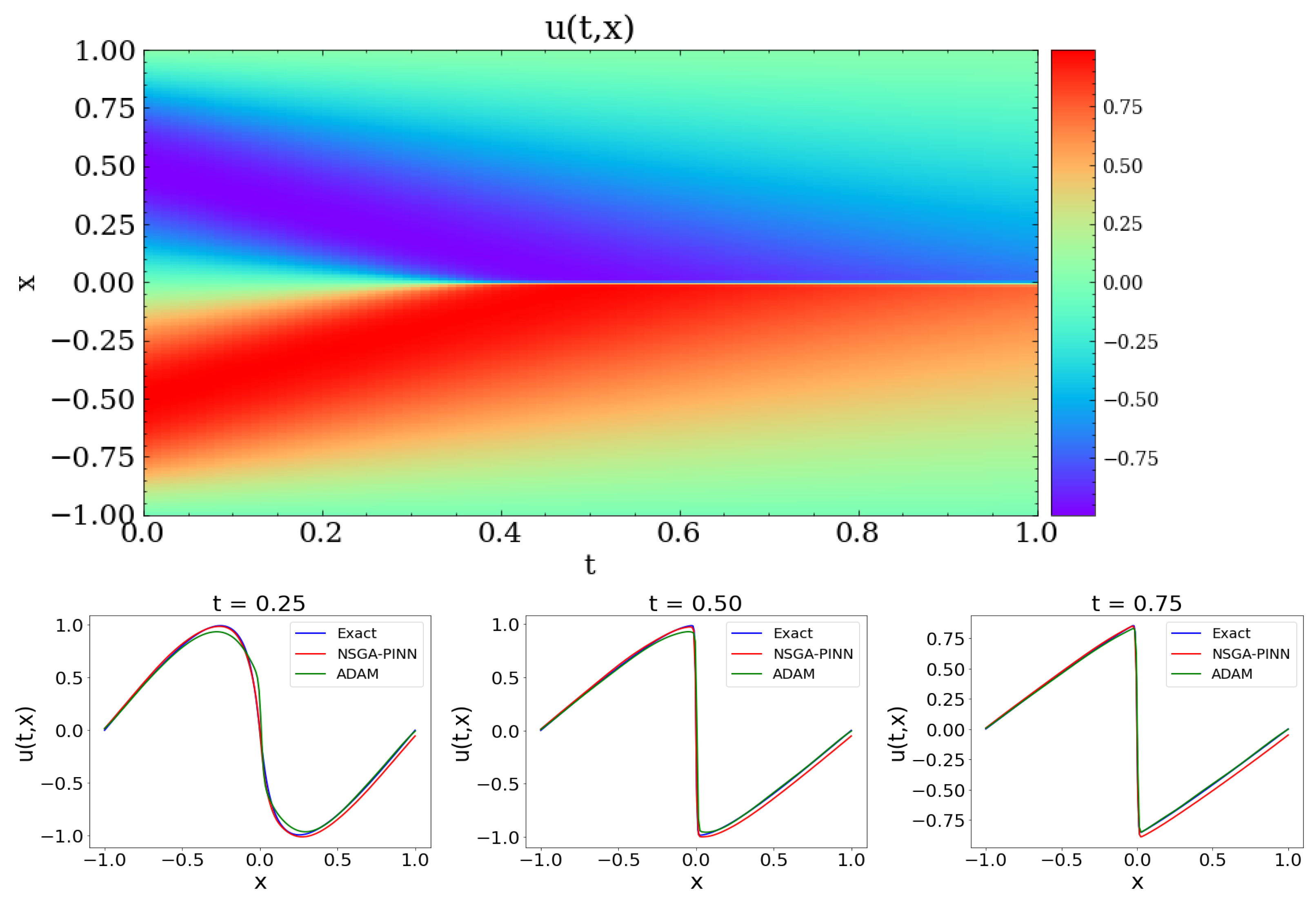
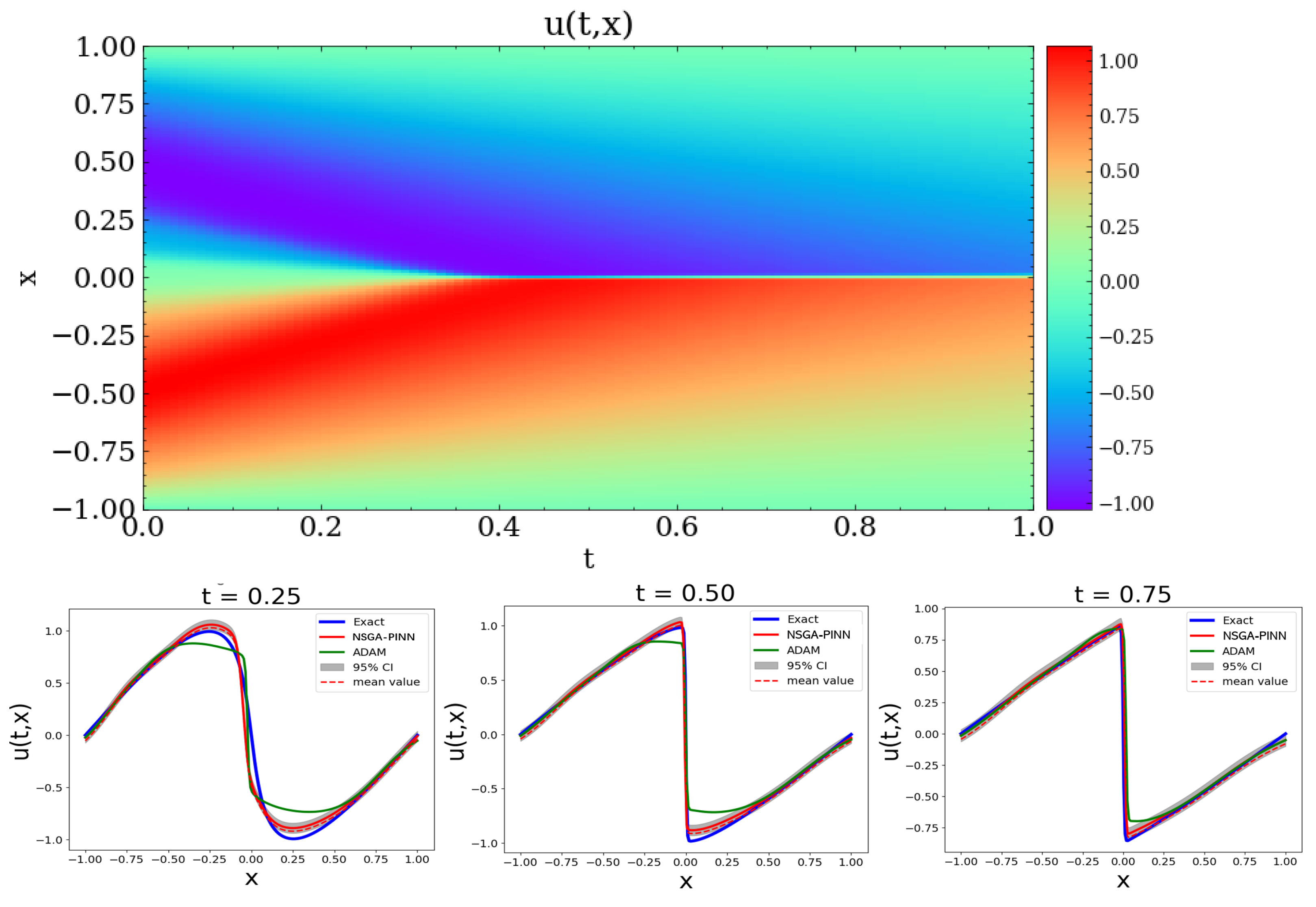
Finally, Figure 8 displays contour plots of the solution to Burgers’ equation. The top figure shows the result predicted using the proposed NSGA-PINN algorithm. The bottom row compares the exact value with the values from the proposed algorithm and the ADAM method at t = 0.25, 0.50, and 0.75. Based on this comparison, both the NSGA-PINN algorithm and the ADAM method predict values that are close to the true values.

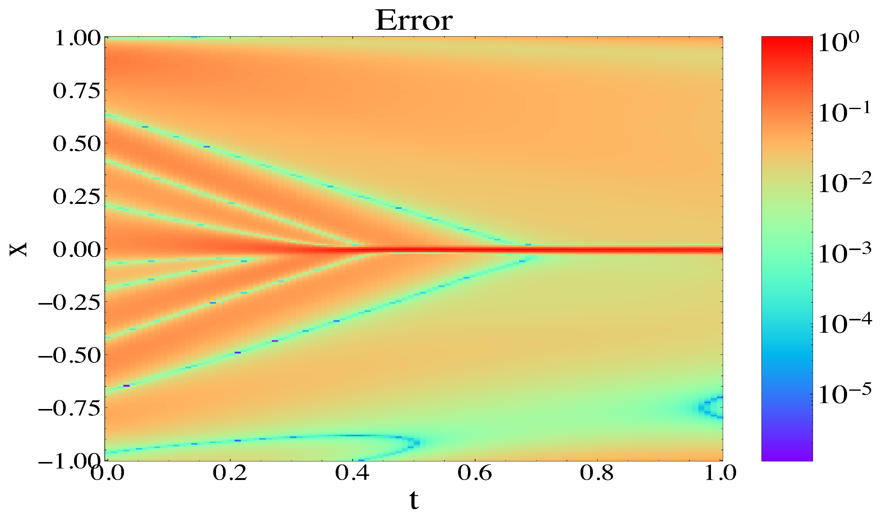
We show the error contour plot for the Burgers equation in Figure 9 to visualize the accuracy of the predicted solution.

4.4. Burgers Equation with Noisy Data

In this experiment, we evaluate the effectiveness of the NSGA-PINN algorithm when applied to noisy data and the Burgers equation. We compare the results obtained from the proposed algorithm with those obtained using the ADAM optimization algorithm. To simulate a noisy scenario, Gaussian noise is added to the experimental/input data. We sample the noise from a Gaussian distribution with a mean value ($\mu$) of 0.0 and a standard deviation ($\sigma$) of 0.1.

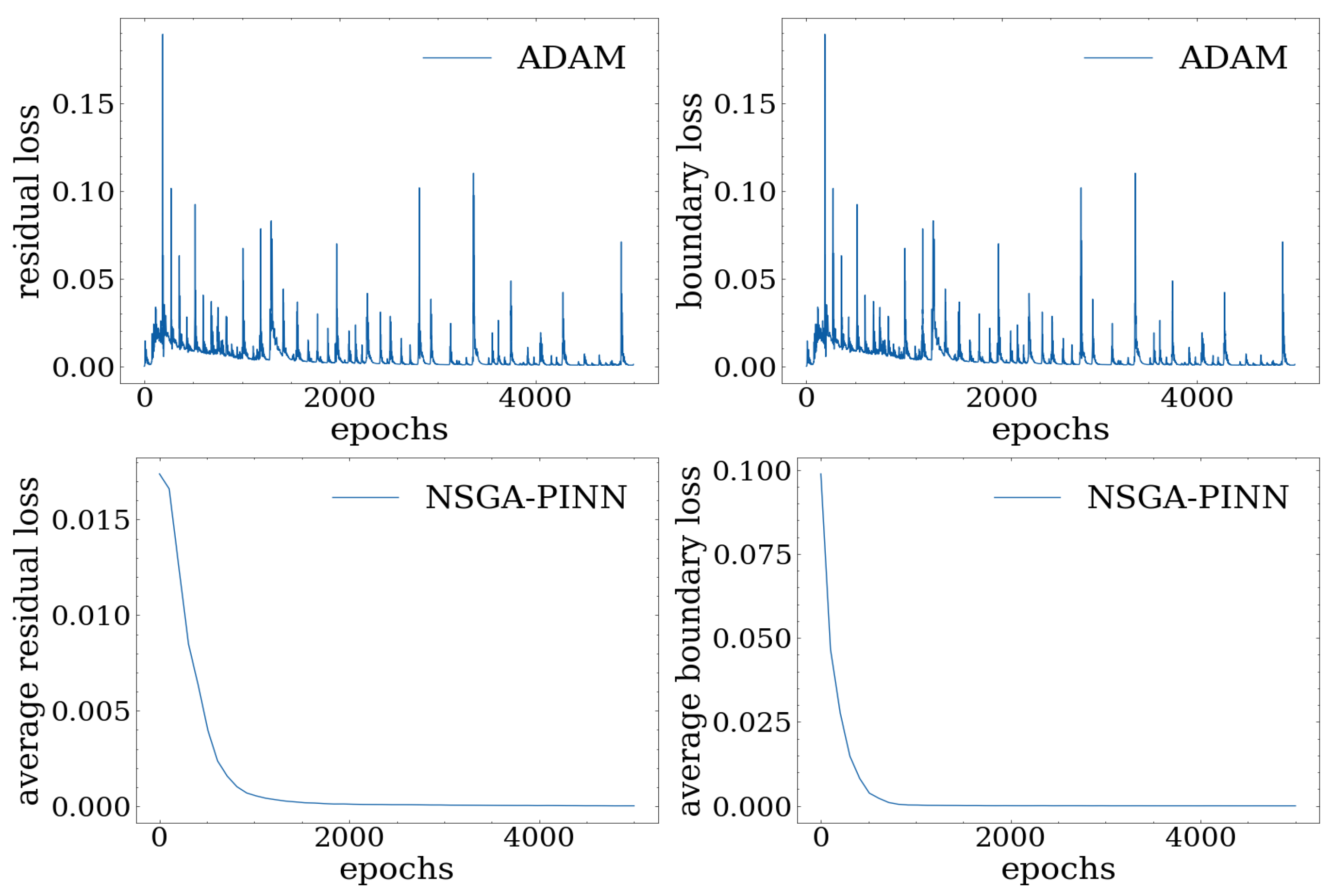
We analyze the effectiveness of the proposed NSGA-PINN method with noisy data. Specifically, Figure 10 and

Table 4. Burgers equation: Comparison of the loss value from NN trained by ADAM method and NSGA-PINN method for Burgers equation with noisy data.

Methods	Residual Loss	Boundary Loss	Total Loss
ADAM	0.0045	0.0481	0.0526
NSGA-PINN	0.0001	0.006	0.0061

illustrate the corresponding loss values. It is worth noting that, while the PINN trained with ADAM no longer improves after 5000 epochs and reaches a final loss value of 0.0526, training the PINN with the proposed algorithm for 20 generations results in a reduced total loss of 0.0061.

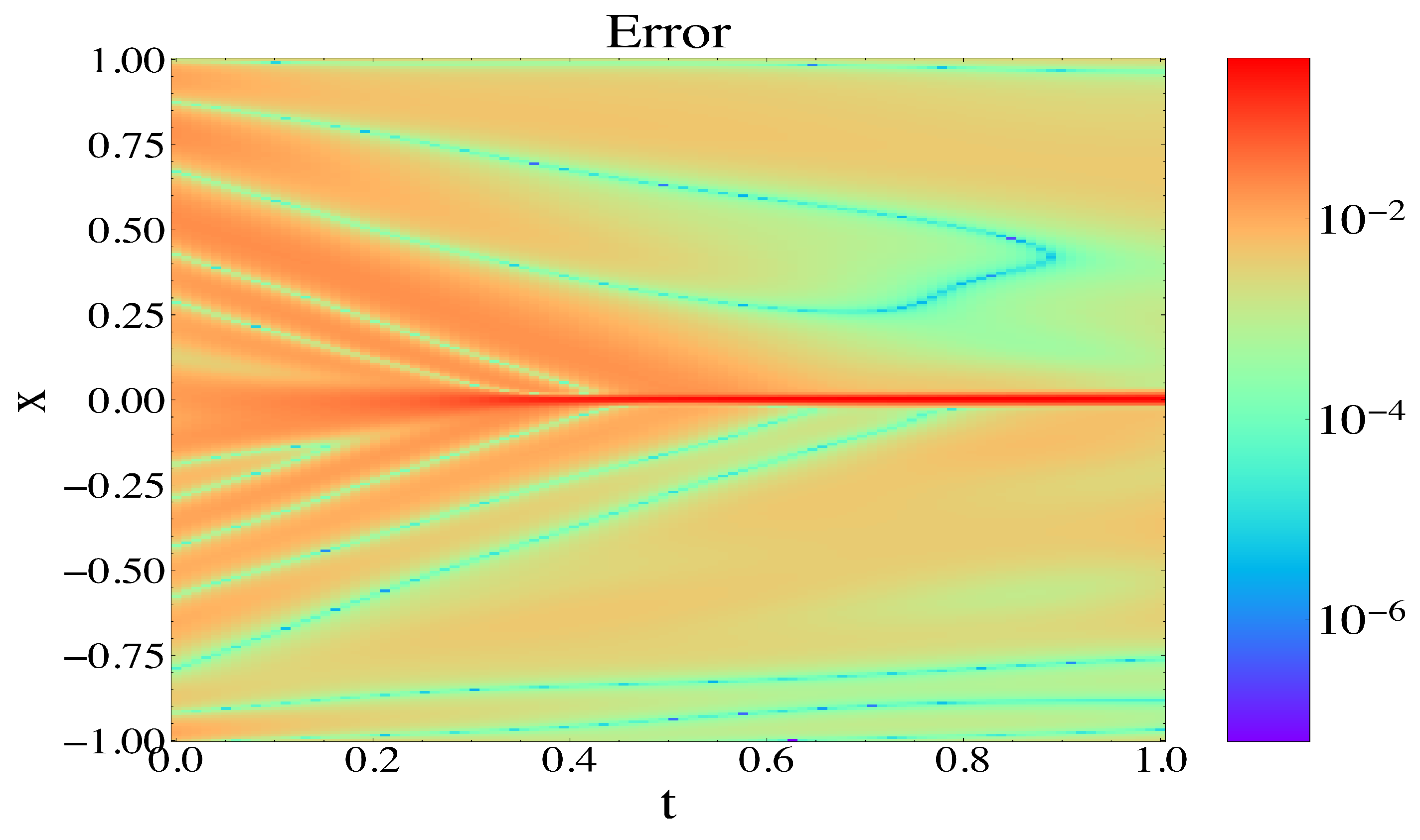
Finally, Figure 11 shows the results of the PINN trained by the NSGA-PINN method with noisy data. The top figure shows a smooth transition over space and time. The lower figures compare the true value with the predicted value for the PINN trained by the proposed method and the traditional ADAM optimization algorithm. The results demonstrate that the prediction from a PINN trained by NSGA-PINN approaches the true value of the PDE solution more closely.

We show the error contour plot for the Burgers equation with noisy data in Figure 12 to visualize the accuracy of the predicted solution.

4.5. Test Survival Rate

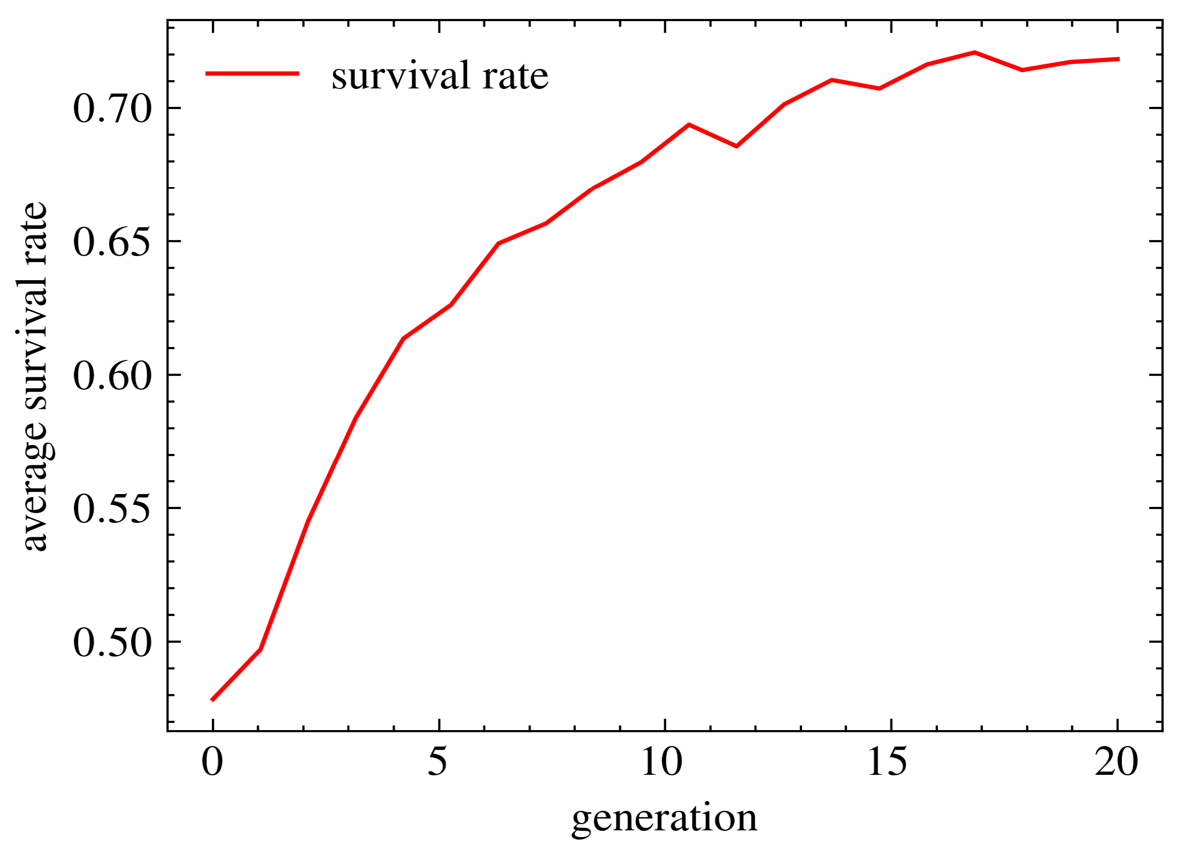
In this final experiment, we conducted further tests to verify the feasibility of our algorithm. Specifically, we calculated the survival rate between each generation to determine if the algorithm was learning and using the learned results as a starting point for the next generation.

The experiment consisted of the following steps: First, we ran the total NSGA-PINN method 50 times. Then, for each run, we calculated the survival rate between each generation using the following formula:

$$\begin{array}{cc}\hfill & S=Q_i/P_i.\hfill \end{array}$$

(12)

Here, $Q_i$ represents the number of offspring from the previous generation, and $P_i$ represents the number of parent population in the current generation. Finally, to obtain relatively robust data that represent the trend of survival rate, we calculate the average value of survival rate between each generation as the algorithm progresses.

Figure 13 shows that the survival rate increases as the algorithm progresses. The survival rate of the first two generations is approximately 50%, but by the end of the algorithm, it improves to 73%. This indicates that our algorithm is progressively learning as subsequent generations are generated, which significantly enhances PINN training.

5. Discussion

The experimental results in the previous section showed promising outcomes for training PINNs using the proposed NSGA-PINN method. As described in Section 3, when solving the inverse problem using the traditional ADAM optimizer, the algorithm became trapped in a local optimum after running for 400 epochs. However, by using the NSGA-PINN method, the loss value continued to decrease, and the predicted solution was very close to the true value. Additionally, when dealing with noisy data, the traditional ADAM optimizer had difficulty learning quickly and making accurate predictions. On the other hand, the proposed NSGA-PINN algorithm learned efficiently and converged to a better local optimum for generalization purposes.

However, the main drawback of the proposed method is that it requires an ensemble of neural networks (NNs) during training. Consequently, the proposed NSGA-PINN incurs a larger computational cost than traditional stochastic gradient descent methods. Therefore, reducing the computational cost of NSGA-PINN is a goal for our future work. For instance, some of the training computational cost could be mitigated by using parallelization. Additionally, we will attempt to derive effective methods for finding the best trade-off between NSGA and ADAM.

More specifically, in our future work, we will focus on balancing the parent population (N), max generation number ($\alpha$), and number of epochs used in the ADAM optimizer. These values are manually initialized in the proposed method. The parent population determines the diversity in the algorithm, and we ideally want high diversity. The max generation number determines the total learning time. Increasing this time allows the algorithm to continue learning from previous generations, but it may lead to overfitting if the number is too large. Note that there is a trade-off between the max generation number and the epoch number used in the ADAM optimizer. A higher generation number allows the NSGA algorithm to perform better, helping the ADAM optimizer escape the local optima, but this comes at a higher computational cost. Meanwhile, increasing the number of epochs used in the ADAM optimizer helps the model decrease the loss value quickly, but it reduces the search space and may lead to the algorithm becoming trapped in the local minima.

6. Conclusions

In this paper, we proposed a novel multi-objective optimization method called NSGA-PINN for training physics-informed neural networks. Our approach involves using the non-dominated sorting genetic algorithm (NSGA) to handle each component of the training loss in PINN. This allows us to achieve better results in terms of inverse problems, noisy data, and satisfying constraints. We demonstrated the effectiveness of NSGA-PINN by applying it to several ordinary and partial differential equation inverse problems. Our results show that the proposed framework can handle challenging noisy scenarios.