In-Process Monitoring of Hobbing Process Using an Acoustic Emission Sensor and Supervised Machine Learning

Abstract

The complexity of products increases considerably, and key functions can often only be realized by using high-precision components. Microgears have a particularly complex geometry and thus the manufacturing requirements often reach technological limits. Their geometric deviations are relatively large in comparison to the small component size and thus have a major impact on the functionality in terms of generating unwanted noise and vibrations in the final product. There are still no readily available production-integrated measuring methods that enable quality control of all produced microgears. Consequently, many manufacturers are not able to measure any geometric gear parameters according to standards such as DIN ISO 21771. If at all, only samples are measured, as this is only possible by means of specialized, sensitive, and cost-intensive tactile or optical measuring technologies. In a novel approach, this paper examines the integration of an acoustic emission sensor into the hobbing process of microgears in order to predict process parameters as well as geometric and functional features of the produced gears. In terms of process parameters, radial feed and tool tumble are investigated, whereas the total profile deviation is used as a representative geometric variable and the overall transmission error as a functional variable. The approach is experimentally validated by means of the design of experiments. Furthermore, different approaches for feature extraction from time-continuous sensor data and different machine-learning approaches for predicting process and geometry parameters are compared with each other and tested for suitability. It is shown that structure-borne sound, in combination with supervised machine learning and data analysis, is suitable for inprocess monitoring of microgear hobbing processes.

1. Introduction

Microdevices are crucial components in diverse, complex products that promise increasingly high growth in many different industries [1]. The most common mechanical microcomponents are microgears, which are used in a wide range of applications, e.g., in the fields of aerospace technology, medical technology, and robotics [2,3]. Microgears have a particularly complex geometry and thus the manufacturing requirements often reach technological limits. In the case of dental instruments such as dental drills, the relatively large geometric deviations of microgears, in comparison to the small component size, have a major influence on the function as well as the generation of unwanted noises and vibrations, which have a direct influence on patients and treating physicians. The main cause is excitations generated during tooth meshing, which are transmitted by means of structure-borne vibrations and radiated as airborne sound. Gear deviations such as profile and flank deviations lead to less than ideal tooth meshing and must therefore be detected and avoided [4,5]. Quality assurance by means of suitable measurement technologies is therefore very important in the context of microgear production.

A comprehensive study by the Physikalisch-Technische Bundesanstalt (PTB) on the potentials and requirements of microgear measuring technology shows, that the quality of the achievable measurement results is not yet sufficient for the high, and in the future further increasing, demands placed on microgear manufacturers [6]. In addition to readily available measurement methods for measuring samples in a measuring room, 100% inline measurements would be necessary to enable control strategies in the sense of a closed-loop approach to further increase the efficiency of the manufacturing processes. The lack of accessibility due to complex geometric features is a major barrier to the use of tactile and optical measurement methods for comprehensive quality assurance of microgears. Furthermore, the long measurement time and the high costs for measuring machines capable of measuring in the single-digit micrometer range represent further barriers to economical 100% inline measurements.

This paper examines the integration of an acoustic emission sensor into the manufacturing process of microgears in order to predict process parameters as well as geometric features. The developed method is investigated with a use case from the dental industry using the example of the gear hobbing process. Hobbing is the most commonly used process for the production of gears. It is a complex process with multidimensional intersections and simultaneous rotation of tools and workpieces. So far, hobbing has been investigated mainly in terms of tool wear. Both electrical current signals [4] as well as airborne sound [7] and structure-borne sound signals [8] are already being used successfully for this purpose. The use of machine learning and data analysis in combination with structure-borne sound signals has the potential to predict the quality of the produced gears. Furthermore, this approach would enable process control in the sense of a closed-loop approach to further increase the efficiency of the hobbing process.

2. State of the Art

2.1. Microgears and the Monitoring of Their Manufacturing Process

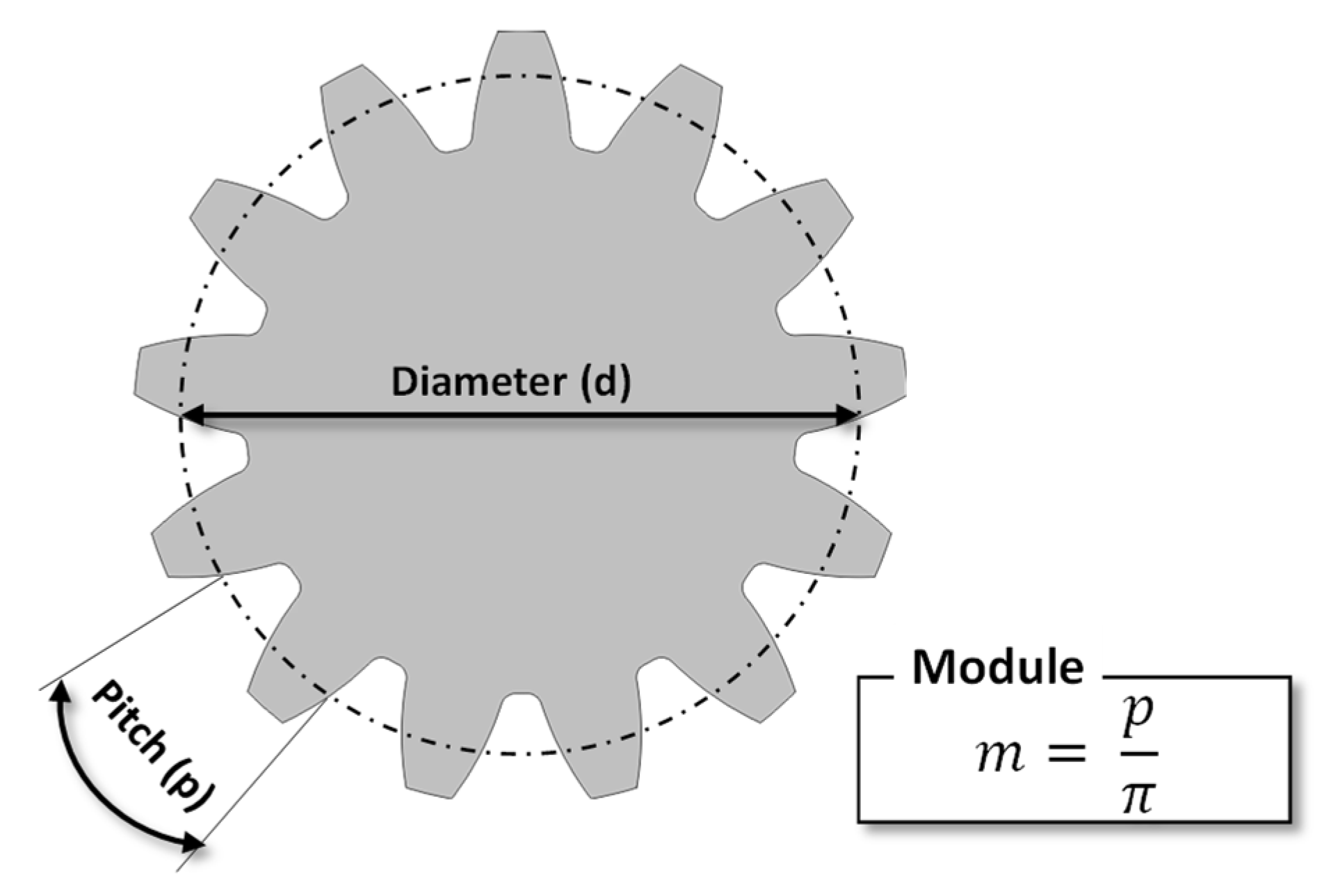
There is no universal definition of microgears, but according to the standard VDI 2731, microgears are defined as gears that have two of the following three characteristics (see Figure 1) [3]:

• Characteristic external dimensions (e.g., diameter or edge length) < 20 mm
• Module < 200 µm
• Structural details < 100 µm

Figure 1. Characteristic gear parameters.

Figure 1. Characteristic gear parameters.

Monitoring the production of micro components requires special, highly sensitive measurement technologies [9]. In addition to traditional measurement technologies, indirect signals can also be utilized for process monitoring. The utilization of current signals from the spindle and feed motors, as described by Ogedengbe et al. [10], has the advantage of being simple and cost effective to measure in comparison to the use of force signals, which contain high levels of noise [11]. Additionally, structure-borne sound signals can provide useful information regarding tool wear [12]. Su [13] further uses structure-borne sound signals for the diagnosis of damaged types of microgears within microdrive systems.

2.2. Condition Monitoring with Structure-Borne Sound

Structure-borne sound is generated by a sudden, localized release of energy, such as in plastic deformation, impacts, friction, or crack formation, and produces mechanical, elastic waves that propagate through solid bodies [14]. Structure-borne sound is measured using the piezoelectric effect as a voltage signal [15]. Due to their smaller dimensions, structure-borne sound sensors are significantly more flexible and less expensive to use than force sensors [16]. Additionally, structure-borne sound sensing is particularly sensitive compared to force sensing and current measurements, which is particularly beneficial when monitoring fine machining processes [17].

Generally, condition monitoring can be divided into monitoring tool wear and tool breakage on the one hand and detecting faulty machine states on the other [18]. Monitoring tool wear is of great importance due to its impact on surface quality and geometric deviations of the manufactured components. The emission of structure-borne sound signals when using worn tools is stronger than when using new tools because wear causes a larger contact surface between the tool and the workpiece. This results in increased friction, leading to increased energy input and increased heat generation [19].

Numerous studies have successfully detected tool wear and breakage using structure-borne sound signals in various manufacturing processes. Marinescu and Axinte [16] investigated tool wear in milling using spectral analysis, revealing significant differences between new and damaged tools. For gear honing, Yum et al. [19] successfully classify tool wear into three classes using features of the frequency domain. Maia et al. [20] use the power spectral density to characterize both tool wear and various wear mechanisms in turning, with an increase in the power spectral density value indicating an increase in wear.

Using structure-borne sound, not only tool wear, but also faulty machine states can be detected, in many cases even identifying the specific damaged component. For example, the structure-borne sound is used to monitor bearings and transmissions, where strong sound emissions are an indication of bearing damage and lubrication loss [18,21]. Additionally, the characterization of various forms of damage in transmissions, such as tooth breakage and pitting, is possible through acoustic emission [22]. Further, structure-borne sound enables the detection of unwanted conditions during turning, such as continuous chip formation, and it enables the investigation of the chip formation process itself [23,24]. Continuous components in the structure-borne sound signal can be associated with plastic deformation and friction between the tool and chip, while chip winding, breaking, and collisions generate burst signals. Additionally, observations show a strong relationship between the RMS value of the acoustic signal and cutting energy.

2.3. Classification of Structure-Borne Sound

Structure-borne sound signals can be combined with various classification methods to predict process parameters or component quality. Wantzen [25] predicted the tool wear of a turning cutter as well as the lubrication condition of sliding bearings and compares the different classifiers. Li et al. [8] also compared different classification methods for predicting tool wear in the hobbing process, with a support vector machine (SVM) producing the best results. Su [13] uses a “Wavelet Neural Network” to predict types of damage to gears in a microdrive, using the wavelet function as an activation function. This resulted in shorter training times, higher prediction accuracy, and reduced convergence problems compared to traditional neural networks.

2.4. Scope of This Work

This research paper builds upon publications that examine the suitability of acoustic signals for mainly monitoring tool conditions. Existing work in the field of hobbing process monitoring is done for macro gears with a focus on utilizing structure-borne sound for condition monitoring and predictive maintenance applications. The current research expands upon these results by investigating the suitability of structure-borne sound signals for monitoring microhobbing processes, as well as the direct monitoring of the quality parameters of complex geometries. This is of particular interest as microgears have a complex geometry and thus the manufacturing requirements often reach the technological limits with no readily available production-integrated measuring methods. The structure-borne sound is captured via intelligent sensor integration. For the data analysis, different classification algorithms are used, which are trained on the basis of labeled data and subsequently tested.

3. Experimental Setup

3.1. Manufacturing Process

The component under investigation is a geared shaft. Its characteristics are specified in

Table 1. Parameters of the investigated microgear.

Parameters	Value
Number of teeth z	13
Width of teeth Wk=3 (3 teeth)	2.188 mm
Module m	0.28 mm
Tip diameter da	4.424 mm
Root diameter df	3.22 mm
Type of gearing	Involute spline according to reference profile DIN 3961
Maximum speed in operation	200,000 min−1

. It is used in dental instruments for power transmission.

The microgear is a standard component of a dental instrument manufacturer and is manufactured using a Tsugami HS207-5ax CNC machine. Hobbing of the teeth is a partial step of the three-minute machining of the finished component and takes 18.9 s. During machining, the workpiece rotates at 150 min⁻¹ and the cutting tool rotates at 1950 min⁻¹.

For the analysis of the tooth quality, only structure-borne sound signals of the hobbing process are considered, during which the teeth are manufactured.

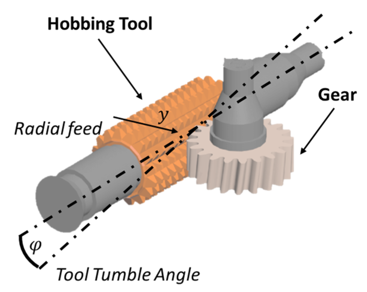
The main process parameters that have an effect on the running process are radial feed and tool tumble (see Figure 2). The radial feed is the distance the tool plunges into the workpiece and the parameter thus has a strong impact on the tooth thickness of the manufactured teeth. The tool tumble, on the other hand, describes the axial tilt of the cutting tool and should be avoided, as it leads to deviations in the tooth profile, and thus reduces the quality of the manufactured teeth. A schematic representation of the parameters is shown in the following figure.

3.2. Sensor Integration

The application of the structure-borne sound sensor greatly affects its signal quality. The location must be chosen so that a direct sound transfer is allowed, with the sound passing through as few interfaces or sound-generating components, such as bearings and gears, as possible. Wang and Liu [23] and Carrino et al. [27] proposed attaching the structure-borne sound sensor to the workpiece, while Inasaki [24] preferred attaching it to the tool with the advantage of a constant distance between the sensor and the cutting point. Variable distances could lead to dynamic damping and distort the signal.

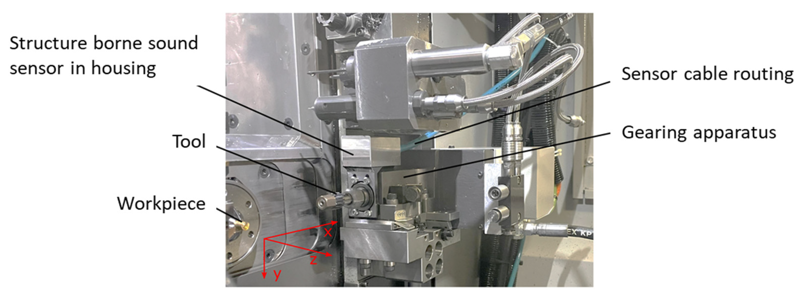
If a direct attachment to the tool and workpiece is not possible, as for our use case due to the small dimensions of the tool and workpiece, Wantzen [25], Maia et al. [20], and Yum et al. [19] suggested attaching it to the tool holder. The chosen attachment of the sensor is shown in Figure 3. In this case, a bracket is mounted with four screws on the gear-hobbing apparatus that holds the cutting tool. The sensor is attached to the bracket with a torque, defined by the sensor manufacturer, of 8 Nm. The surface where the sensor touches the bracket has a low roughness to ensure optimal sound transmission and constant coupling conditions [28]. The wire for data transmission is guided from the machine to the preamplifier using a pneumatic hose. To protect against environmental influences such as chips and oil, the structure-borne sound sensor has a housing consisting of two bent and bonded aluminum parts. This allows for optimal sealing while simultaneously reducing the weight of the bracket.

The integration of the sensor, including the mount and cover in the machine, can be seen in Figure 4.

3.3. Data Acquisition

In order to capture the structure-borne sound signal, a piezoelectric sensor from the company QASS is used. This sensor records the high-frequency vibrations generated during hobbing and converts them into an electrical signal. This signal is then routed through a cable to the preamplifier and then to the Optimizer4D, an evaluation unit. A study by Gauder et al. has demonstrated that microgear measurements using focus-variation technology can achieve low, single-digit micrometer measurement uncertainties [29]. Based on the findings of Gauder et al., the geometric reference measurements are performed analogously using an optical coordinate measuring machine “µCMM” from Bruker Alicona. To do this, the manufactured microgear is placed in ethanol and cleaned to exclude any measurement deviations caused by contamination. The coordinate measuring machine works on the principle of focus variation. Light is projected onto the measurement object and reflected from its surface. The reflected light is focused by precision optics and hits a light-sensitive sensor. Depending on the distance of the sensor from the component surface, only certain areas of the component are in focus. By moving the sensor vertically and analyzing the sharpness of different areas, the topography of the component surface can be reconstructed. In this way, point clouds of the gear geometry are created in a four-minute measurement program, from which the gear characteristics such as profile deviations, flank line deviations, and transmission errors, are calculated using commercial gear inspection software “Reany”.

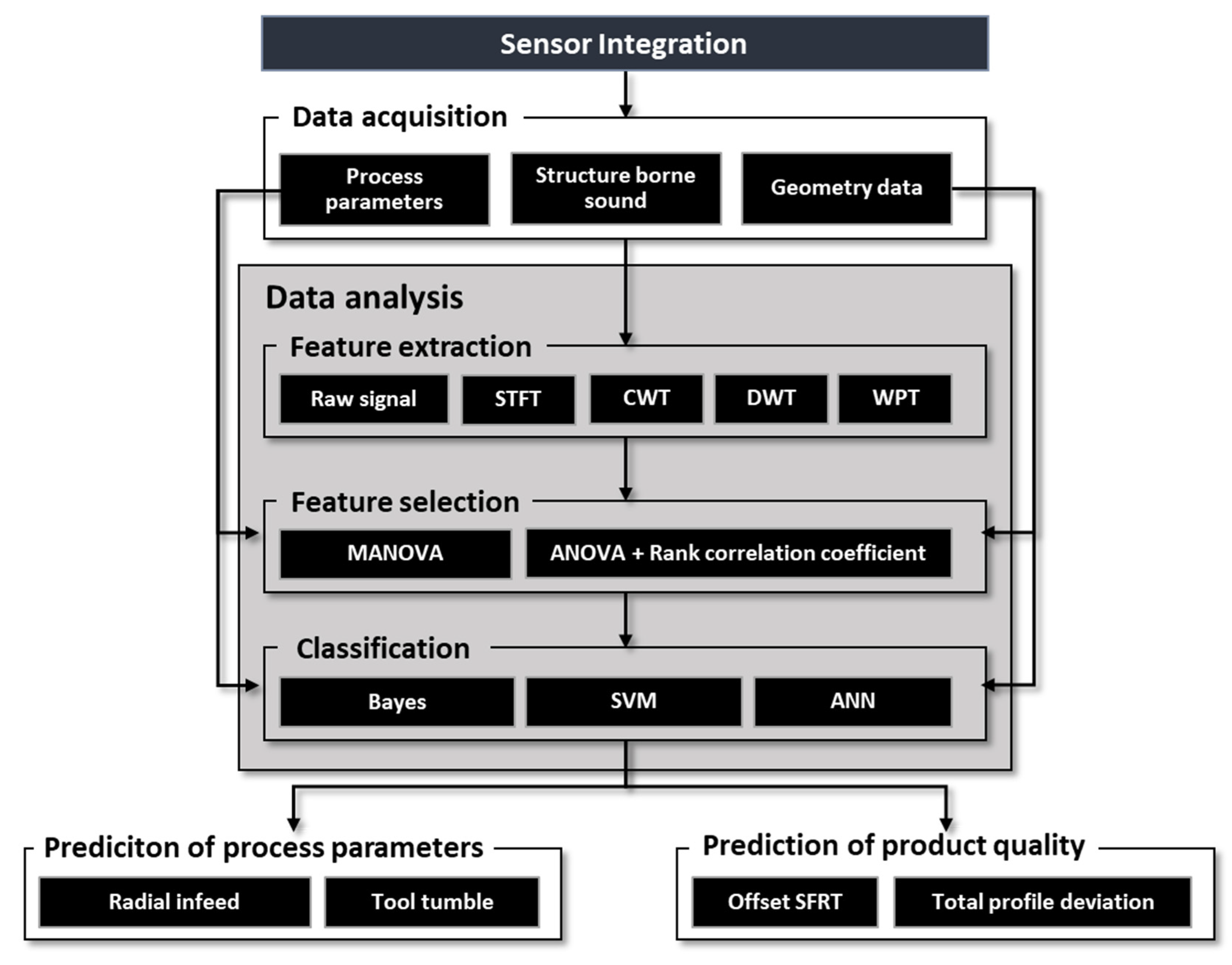
The structure-borne sound and geometry data, as well as the specified process parameters of the experiment, are fused together and evaluated in Matlab (see Figure 5).

4. Methodology

In previous work, various sensor integration layouts were compared using a cost–benefit analysis in terms of signal quality, sensor accessibility, and sensor protection from chips and oil. The selected layout is described in Section 3.2. In the “Data Acquisition” step, structure-borne sound signals of the hobbing process are subsequently recorded using the design of experiments, which will serve as the data basis. To investigate the relationship between the structure-borne sound signals and the process parameters or the quality of the manufactured gears, the process parameters of tool tumble and radial feed are varied in a full factorial experimental design. The geometry of all manufactured microgears is then optically measured and evaluated according to standard DIN ISO 21771. The data-analysis approach follows the procedure presented by Mikut [32] for designing a data-mining method as shown in Figure 6. Initially, features are extracted from the structure-borne sound signals. These are calculated both from the time signal itself and from various spectral analyses such as short-time Fourier transform (STFT), continuous wavelet transform (CWT), discrete wavelet transform (DWT), and wavelet packet transform (WPT). In the feature selection, two different approaches are applied. Features are selected using both multivariate analysis of variance (MANOVA) and a combined method of analysis of variance (ANOVA) and rank correlation coefficient for redundancy reduction. As input variables, the features extracted from the raw signal and the features of one spectral transformation are used together to evaluate the suitability for classification. The restriction to use only features of one spectral transformation in addition to features of the raw signal is for efficiency reasons. Both the prediction of process parameters as well as quality variables are investigated using three different classification methods: a Bayes classifier, a support-vector machine, and a k-nearest-neighbor classifier. These are evaluated and compared based on their prediction accuracy.

4.1. Design of Experiments

In the test, the parameters of tool tumble and radial feed were varied. The radial feed influences the distance the tool plunges into the workpiece, and therefore has a direct influence on tooth thickness, which is a central parameter for gears. The tool tumble describes the axial inclination of the milling tool and leads to unwanted deviations of the profile line. With large tumble values, the profile line deviates more strongly from its nominal curve, since the skewing of the tool produces wavy tooth flanks. A full-factorial experimental design is used so that data is recorded for each combination of radial feed and tool tumble settings. Four equidistant steps are used to vary the tumble between 0 µm and 21 µm. Measuring the tumble with a dial gauge only allows the setting of a tumble value close to 0 μm. This setting of minimum tumble will be referred to as tumble class 0 μm in the following. For each tumble step, the radial feed is varied in five steps between −0.02 mm and +0.02 mm in randomized order, with each parameter set being repeated ten times. A total of 200 components were manufactured with 20 different combinations of tumble and radial feed settings. The structure-borne sound signals are recorded at a sampling frequency of 3.125 MHz, which, according to the sampling theorem, allows frequencies up to 1.5625 MHz to be investigated.

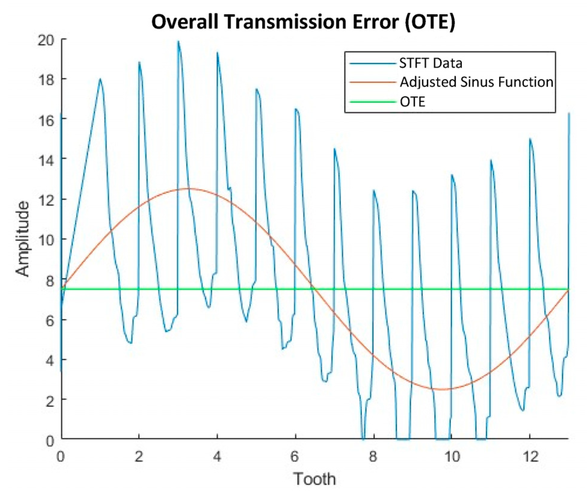
By varying the radial feed and the tool tumble, the relationship between the process parameters, the emitted structure-borne sound, and the component quality of the manufactured gears are investigated. The question to be answered is whether structure-borne sound measurements offer the potential to predict the two process parameters tool tumble and radial feed directly in the process. In the next step, it is to be investigated whether structure-borne sound signals, in addition to the process parameters, also allow direct conclusions to be drawn about the component quality. The quality variables used here as examples to characterize the component quality of gears are the median-profile total deviation over all teeth (see DIN ISO 1328-1 [33]) and the offset of the single flank rolling test (STFT), which is defined as the overall transmission error (OTE) in the further discussion. Both values refer to the left tooth flanks. The median profile total deviation over all teeth was chosen since it is one of the most characteristic parameters for describing gears. The OTE, on the other hand, was chosen since it can be calculated from the deviation of rotation measured in the STFT (Figure 7 in blue) during one revolution of the microgear (13 teeth), which represents a functional test of gears. If a sine function is fitted into this data (red curve), the deviation of the axis around which this sine oscillates (green) from the axis without rotation deviation describes the OTE.

With increased tooth thickness, the master gear and the tested microgear are engaged earlier in the STFT, resulting in a large rotational-angle deviation and a larger OTE. For the later classification of the geometry data, five classes of the OTE and four classes of the total profile deviation are defined in an equidistant discretization. Classes are then assigned to the value-continuous quality data.

4.2. Data Analysis

4.2.1. Feature Extraction

The reliability of the prediction of output variables such as tool wear, process parameters, or component quality depends on the quality of the extracted features [8]. The vast majority of research already conducted extracts features using spectral analysis [16,25,27]. Extraction from time signals is also used [8,25,34,35]. An overview of the features used in the aforementioned works can be seen in

Table 2. Selection of possible features in the time and frequency domain according to Mikut [32], Wantzen [25], Li et al. [8], and Meng-Kun Liu et al. [34].

Time Domain	Frequency Domain
Mean value of the amplitudes RMS value of the amplitudes (energy equivalent) Standard deviation of the amplitudes Maximum/minimum of the amplitudes Signal energy Sum of all amplitudes Span between maximum and minimum amplitudes Mean value of the envelopes of all amplitudes Skewness Kurtosis	Mean value of the amplitudes of a frequency band RMS value of the amplitudes of a frequency band Signal energy of a frequency band Maximum/minimum amplitude Frequency of maximum/minimum amplitude Percentile Mean value of the 1st derivative of the signal

.

Wantzen [25] extracted features from both the time and frequency domains using the short-time Fourier transform (STFT) and the wavelet transform (WT). Since the features extracted using STFT and from the time domain carry more relevant information, they are selected more frequently than the WT features in the feature selection discussed below. Meng-Kun Liu et al. [34] also extracted statistical features such as the RMS value, mean, standard deviation, and maximum values from the spectrum using the wavelet packet transform (WPT).

The feature types used here can be seen in

Table 3. Types of extracted features from the raw signal and time-frequency spectra.

Raw Signal	Total Time-Frequency Spectrum	Per Frequency Band of the Time-Frequency Spectrum
Maximum and minimum amplitudes as well as their occurring timestamp Range Mean value Standard deviation RMS value Signal energy Signal power	Maximum and minimum amplitude as well as their frequency and time of occurrence Mean value Median Standard deviation RMS value	RMS value Mean value Standard deviation Median

. These are chosen due to their good results in the literature. Features of the recorded structure-borne sound signals are extracted both from the raw signal itself and from the time-frequency spectra of various spectral analyses.

In addition to the short-time Fourier transform, the best-known spectral transform, various types of wavelet transforms are used here for feature extraction. Compared to STFT, these have the advantage that the resolution is not constant in the time-frequency domain. This results in a fine-frequency resolution at low frequencies, which becomes coarser as the frequency increases. With the wavelet packet transform (WPT) the resolution can even be adapted to the signal under consideration. For theoretical background, the reader is referred to Puente León 2019 [36]. For feature extraction, the time-frequency spectra STFT, a continuous wavelet transform (CWT), a discrete wavelet transform (DWT), and the WPT with two different resolutions (15 and 128 coefficients), are used here.

Features can be extracted from the complete time series as well as from single intervals. Marinescu and Axinte [16] analyze the spectrum of effective cutting times at which the tooth of the tool is engaged. As a result, less data has to be transformed into the time-frequency domain, which increases the efficiency of feature extraction.

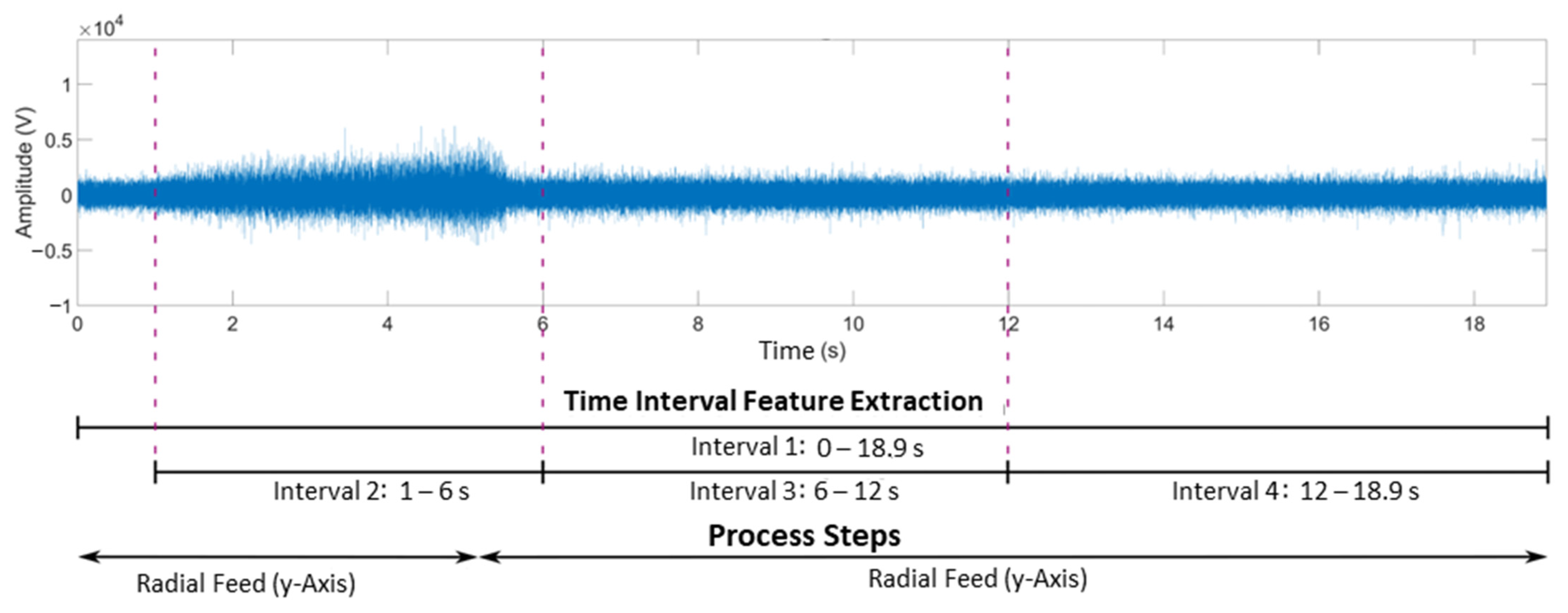
A time interval of either the raw signal or a spectrum is used here to determine a feature. Four time intervals are defined for feature extraction. Time interval one covers the entire hobbing process, while time intervals two to four cover only partial sections. The division into different time intervals allows the individual phases of the process to be considered separately and their characteristics to be examined individually. In this way, characteristics that only occur in one of the process steps become visible. The extracted feature is named based on the underlying data form (raw signal or spectral transform), its type, and the time interval used.

A raw signal acquired at 0 µm tumble and a radial feed of 0 mm and the time intervals used can be seen in Figure 8.

4.2.2. Feature Selection

Since a large number of features would negatively influence the computation time and would not improve the classification result due to redundant information, a feature selection is performed.

There are many different approaches to feature selection in the literature. Wantzen [25] and Yum et al. [19] selected suitable features for classification using an analysis of variance. Here, features are either evaluated individually based on their suitability for classification (ANOVA), or the best feature combination is searched for iteratively (MANOVA) (see [32]). To further reduce the number of features and redundancy, Yum et al. [19] combined correlated features and thereby achieve a 4.2% increase in tool wear prediction accuracy. Li et al. [8], on the other hand, fused the extracted features using principal component analysis. The features selected in this way achieved significantly better classification results than using all extracted features.

All extracted features of the raw signal and one spectral transform each are used as input for feature selection. Since the raw signal, which is the basis of the spectral transformations, is always recorded, raw signal features are always used. For reasons of efficiency, only one spectral transformation is to be calculated in the application and its features are to be used. Two alternative methods of feature selection, MANOVA and a combination of ANOVA and rank correlation coefficient r_s, are used to select information-bearing features from the input variables, which allow a good separability of the output variables into their classes. For the four output variables of radial feed, tool tumble, OTE, and total profile deviation, suitable feature combinations are selected separately in each case.

The first feature selection method investigated selects the best feature combination for classification using MANOVA. Depending on the considered output variable, different numbers of features are selected by the MANOVA.

In the second feature selection procedure investigated, the features evaluated in the ANOVA are sorted according to their suitability for classification, and redundant features are removed. Only features with a rank correlation coefficient of less than 0.5 are retained. Thus, the highest-ranked 60 least redundant features per combination of raw signal features and features of a spectral transformation were selected.

4.2.3. Classification

The whole data set contains 200 structure-borne sound signals at 20 different combinations of radial feed and tool tumble. Seven structure-borne sound signals of each of the ten repetitions per parameter setting are used as labeled learning data sets for the model training (140 structure-borne sound signals). Three signals per parameter setting (60 structure-borne sound signals) are randomly selected, excluded from model training, and later classified with the trained model in order to validate the models found. All data are also variance normalized.

For the classification of the process parameters and quality parameters, three different classification methods are tested with the selected features. The chosen methods, the Bayes classifier, the support vector machine, and the nearest-k-neighbor classifier, are selected since they are commonly used in literature and based on different principles. While in the Bayes classifier, the decision is made probability based and in the SVM the best separation plane to separate the different classes is searched in an optimization problem. In the KNN classifier, unknown data points are compared with similar (small-distance or large-correlation coefficient) training objects.

The models of the classification methods are trained using the learning data set in fivefold cross validation. The standard hyperparameters of the different models (see

Table 4. Varying model parameters in the search for the optimal classification model.

Bayes Classifier	SVM	KNN Classifier
Data distribution	Training method for multiclass problems Kernel function, kernel scale Weighting factor (penalization of misclassification)	Number of nearest neighbors Distance measure Distance weighting

) are varied in 30 iterations. In an automatic optimization, the classification model with the minimum classification error is searched for.

The model found is then used to predict the output variables of the validation data set. With the evaluation measure, accuracy, the models trained per feature combination and classification method are evaluated with respect to their suitability for the prediction of the respective output variable. The calculation of the accuracy can be seen in Equation (1). The evaluation allows statements about which combination of feature extraction and selection, as well as classification methods for the prediction of process parameters and quality variables, are potentially promising in the practical application.

$$\mathrm{accuracy}=\frac{\mathrm{TP}+\mathrm{TN}}{\mathrm{TP}+\mathrm{FP}+\mathrm{TN}+\mathrm{FN}} \mathrm{with} \begin{array}{l}\mathrm{TP}:\mathrm{True}\mathrm{positive}\\ \mathrm{FP}:\mathrm{False}\mathrm{positive}\\ \mathrm{TN}:\mathrm{True}\mathrm{negative}\\ \mathrm{FN}:\mathrm{False}\mathrm{negeative}\end{array}$$

(1)

5. Results

5.1. Suitability of Structure-Borne Sound for Monitoring the Hobbing Process

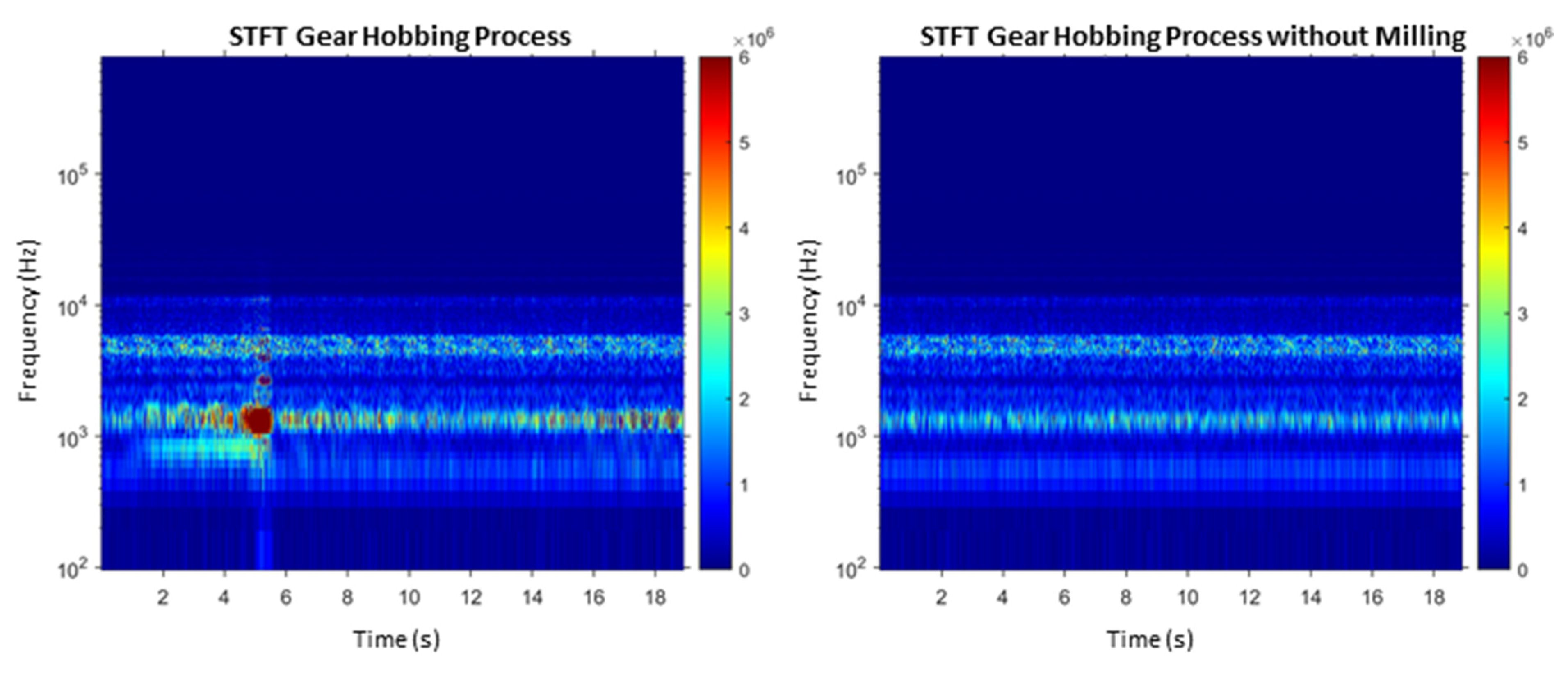
To check whether the measured structure-borne sound contains information about the hobbing process, structure-borne sound signals are recorded in each case with and without the engagement of the milling tool. In this way, it is possible to determine which characteristics of the spectrum are generated by the gear hobbing process.

In the spectra generated by means of the STFT in Figure 9, it can be seen that the spectra with and without hobbing intervention differ significantly in the frequency range of 400–2000 Hz. These differences are caused by the material removal during the gear manufacturing process. The frequency spectrum shows a high amplitude of the frequency 487.5 Hz. This corresponds to the tooth engagement frequency of the milling tool. The engagement of the teeth of the tool results in an energy input, which leads to increased amplitudes of the structure-borne sound signal. It is thus shown that the sensor integration used enables the measurement of the structure-borne sound generated during hobbing.

The frequencies contained in the spectrum without milling intervention originate from the ambient influences and can possibly be assigned to oil cooling, bearing and gear vibrations of the tool, workpiece spindle or vibrations of the coolant pump, the power supply, and any ambient noise. The environmental influence will not be further investigated here.

5.2. Analysis of the Spectra for Varying Process Parameters

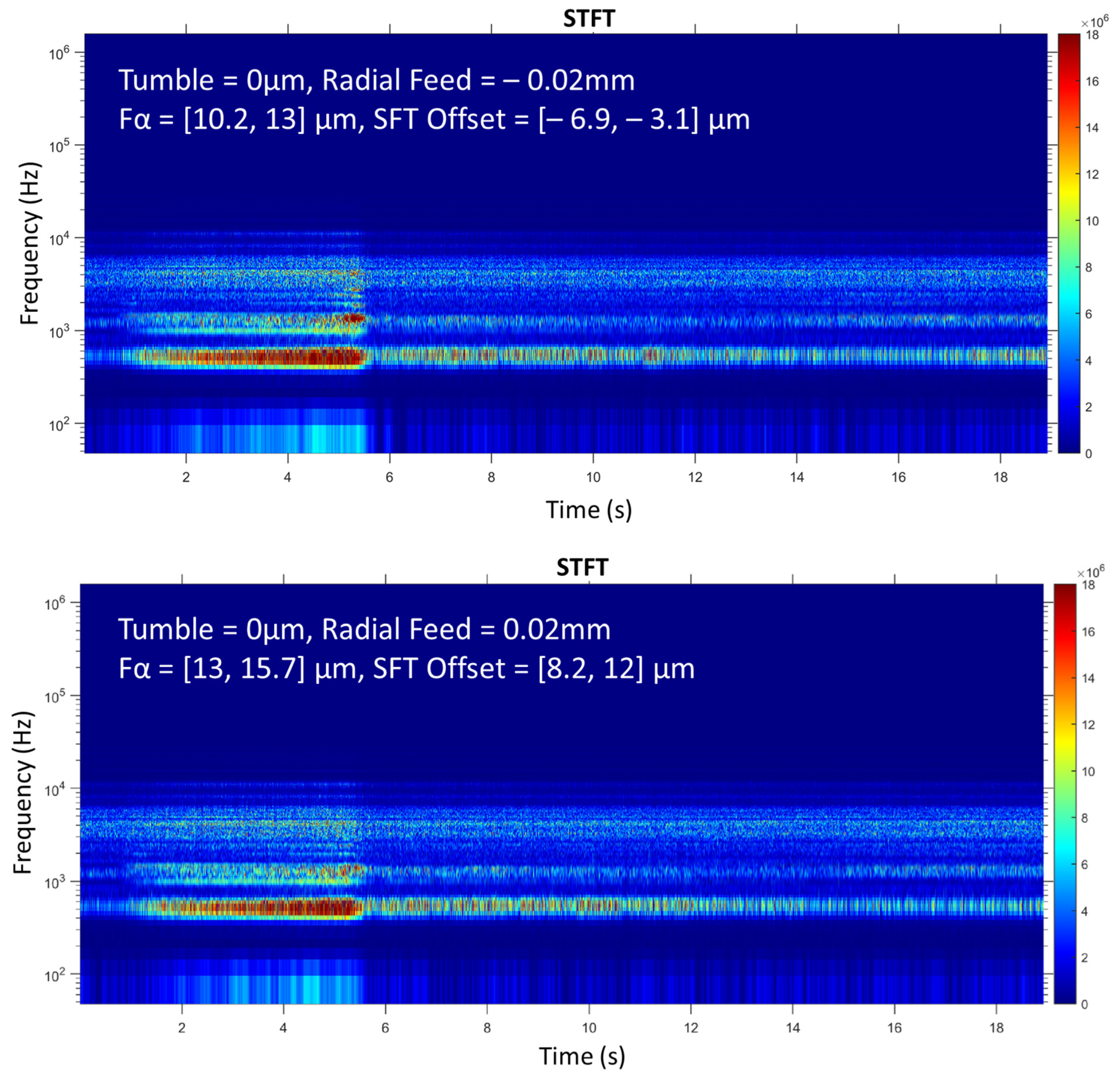
Figure 10 shows the STFT spectra of different settings of the radial feed process parameter at a tumble of 0 µm. In order to determine whether visual differences between the spectra of the different process parameters can be detected, extreme values are considered. For completeness, the classes of the total profile deviation Fα and the OTE are also given.

The spectrum with a radial feed of −0.02 mm has a higher energy effect in the frequency range 1000–2000 Hz between second four and second six and in the frequency range 400–700 Hz between second 12 and second 18 due to higher amplitude values than the spectrum of the radial feed of 0.02 mm. This can be explained by the fact that at the smallest step of the feed, the tool and workpiece have the smallest distance from each other. Thus, the cutter penetrates deeper into the workpiece, has a larger contact area, and consequently provides a larger energy input than the other stages of the radial feed, where the penetration depth is smaller.

Cross influences between the radial feed and the tumble can be assumed, however, they are not considered here due to the separate classification of the process parameters and quality data. Further disturbing influences such as the temporal change of the tumble and tool wear during the test execution probably also influence the structure-borne sound signal and the spectra calculated from it. The heating of the machine and the resulting temperature influences can be ruled out since the machine had already warmed up before the start of the tests and after the tumble stage was changed.

Since hardly any differences between various process parameters and quality variables can be seen with the naked eye, features are extracted from the spectra as described in the methodology.

5.3. Classification Results

Three different classification methods are used to predict the process parameters, radial feed, and tool tumble. For each selected feature combination, models of the three classification methods are trained for each output variable. The validation results of these models are presented in the following.

5.3.1. Radial Feed

For the classification of radial feed into five equidistant steps from −0.02 mm to 0.02 mm, the values of the accuracy of the different classification methods with different feature combinations are shown in

Table 5. Evaluations of the classification models for the classification of radial feed.

Feature Selection	Number of Features	Accuracy Bayes	Accuracy SVM	Accuracy KNN
MANOVA RS + STFT	1	0.60	0.53	0.55
MANOVA RS + CWT	1	0.60	0.67	0.62
MANOVA RS + DWT	1	0.68	0.69	0.62
MANOVA RS + WPT with 15 coeff.	1	0.83	0.88	0.83
MANOVA RS + WPT with 128 coeff.	1	0.83	0.83	0.85
ANOVA + rs RS + STFT	60	1.00	1.00	1.00
ANOVA + rs RS + CWT	60	1.00	1.00	1.00
ANOVA + rs RS + DWT	60	0.97	1.00	1.00
ANOVA + rs RS + WPT with 15 coeff.	60	0.70	1.00	0.97
ANOVA + rs RS + WPT with 128 coeff.	60	0.98	1.00	1.00

.

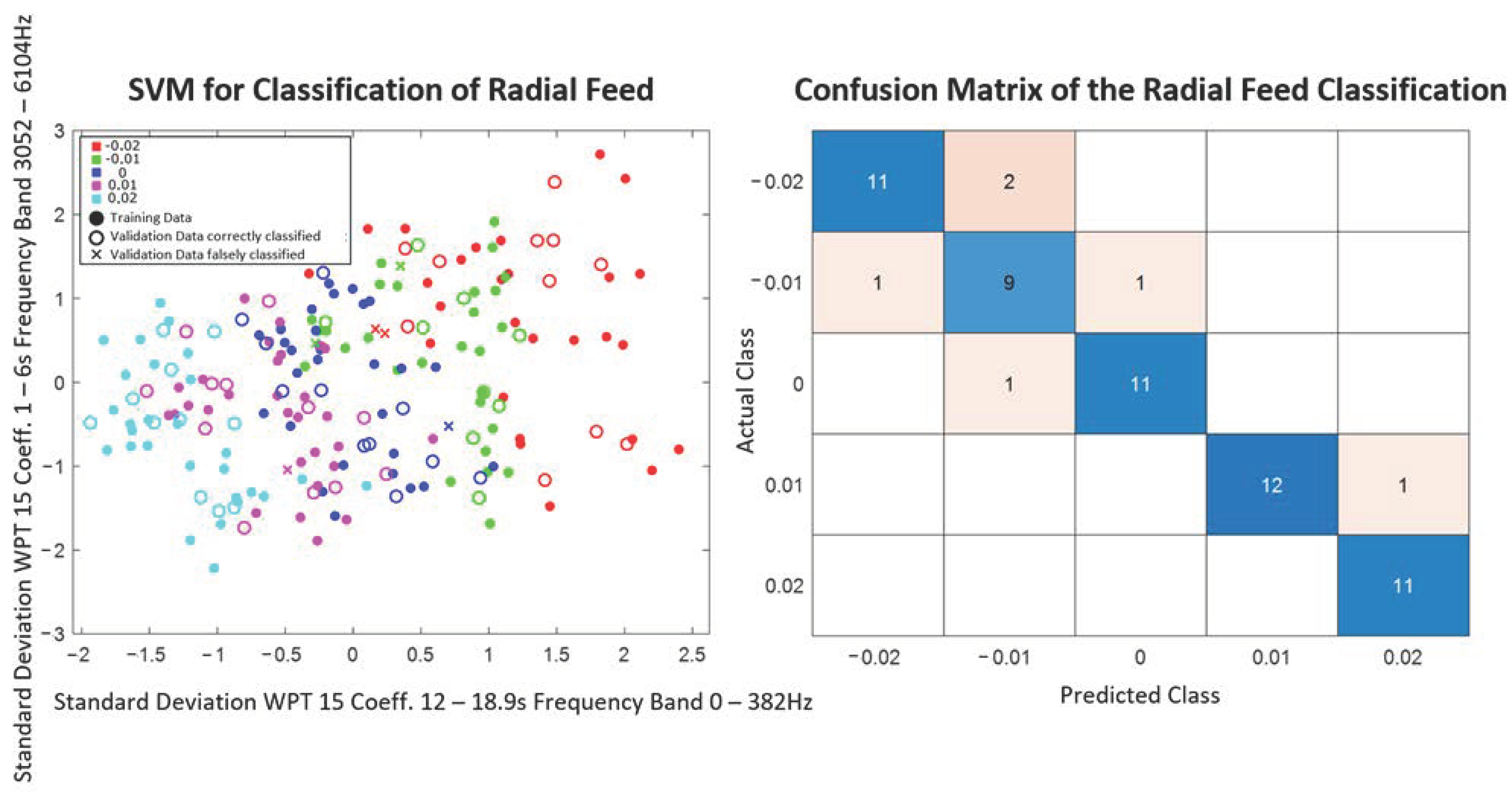
For the classification of the radial feed, the SVM is best suited with the highest accuracy of 0.9, which works with five features of the raw signal determined by MANOVA and the WPT with 15 coefficients. The learning data set and the predicted output variables of the best two of these five features can be seen in Figure 11, as well as the confusion matrix of the SVM on the right. The plot of the best two of the five features used only gives an impression of the separability of the different classes, but not of the class boundaries in the five-dimensional space. The confusion matrix is a method to assess the quality of a classification model in machine learning. It visualize the number of predictions that were correct or incorrect. The numbers entered in the main diagonal correspond to the number of correctly classified test data. The color scale (from blue to red) represents the proportion of correctly and incorrectly classified data.

From the confusion matrix, it can be seen that misclassifications are only assigned to adjacent levels of radial feed, but not to levels further away. The reason for this can be the overlapping of the different classes in the multidimensional feature space, whereby no clear separation plane can be found. Consequently, misclassifications occur in the border area.

The other features selected using MANOVA are also able to correctly classify at least 83% of the validation data when using an SVM. The KNN method, on the other hand, is poorly suited for predicting radial feed, especially in combination with feature selection using ANOVA and the rank correlation coefficient, since only low accuracy values are achieved. The features of the raw signal selected by ANOVA and the DWT also provide low accuracy values for the classification with the KNN method as well as when using an SVM.

5.3.2. Tool Tumble

The validation results of the Bayes classifiers, SVMs, and KNN classifiers trained for tool tumble prediction per feature combination are shown in

Table 6. Classification model evaluations for tool tumbling classification.

Feature Selection	Number of Features	Accuracy Bayes	Accuracy SVM	Accuracy KNN
MANOVA RS + STFT	1	0.60	0.53	0.55
MANOVA RS + CWT	1	0.60	0.67	0.62
MANOVA RS + DWT	1	0.68	0.69	0.62
MANOVA RS + WPT with 15 coeff.	1	0.83	0.88	0.83
MANOVA RS + WPT with 128 coeff.	1	0.83	0.83	0.85
ANOVA + rs RS + STFT	60	1.00	1.00	1.00
ANOVA + rs RS + CWT	60	1.00	1.00	1.00
ANOVA + rs RS + DWT	60	0.97	1.00	1.00
ANOVA + rs RS + WPT with 15 coeff.	60	0.70	1.00	0.97
ANOVA + rs RS + WPT with 128 coeff.	60	0.98	1.00	1.00

.

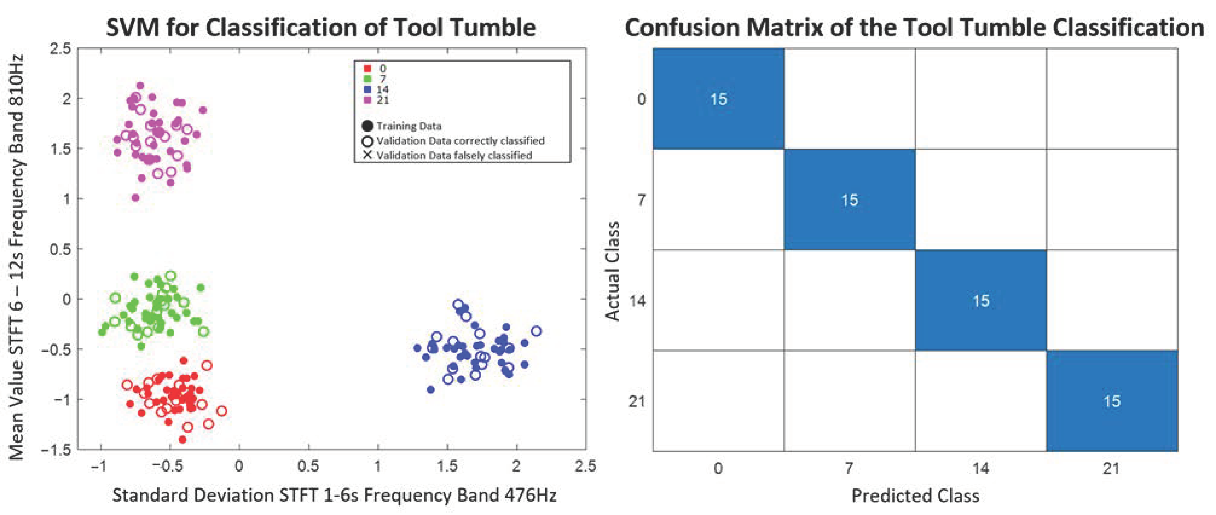
All feature combinations selected with ANOVA and the rank correlation coefficient can separate the validation data into the four tumble classes without error with an SVM. The feature combination of raw signal and STFT, as well as raw signal and CWT, can even make error-free predictions with all three classification methods examined. For the two best evaluated of the 60 selected features from the raw signal and the STFT, the training and predicted validation data of the SVM and its confusion matrix are given in Figure 12. The features selected by MANOVA from the raw signal and STFT cause the most classification errors with all trained models. The worst prediction is made by the SVM, which achieves an accuracy of 0.53.

5.3.3. Transmission Error

The scores of the classifications with different feature selections using different classification methods are shown in

Table 7. Classification model evaluations for OTE classification.

Feature Selection	Number of Features	Accuracy Bayes	Accuracy SVM	Accuracy KNN
MANOVA RS + STFT	4	0.69	0.88	0.69
MANOVA RS + CWT	5	0.57	0.86	0.78
MANOVA RS + DWT	8	0.79	0.83	0.67
MANOVA RS + WPT with 15 coeff.	6	0.74	0.78	0.79
MANOVA RS + WPT with 128 coeff.	5	0.67	0.84	0.72
ANOVA + rs RS + STFT	60	0.76	0.81	0.60
ANOVA + rs RS + CWT	60	0.59	0.72	0.59
ANOVA + rs RS + DWT	60	0.52	0.43	0.45
ANOVA + rs RS + WPT with 15 coeff.	60	0.57	0.53	0.36
ANOVA + rs RS + WPT with 128 coeff.	60	0.72	0.64	0.62

.

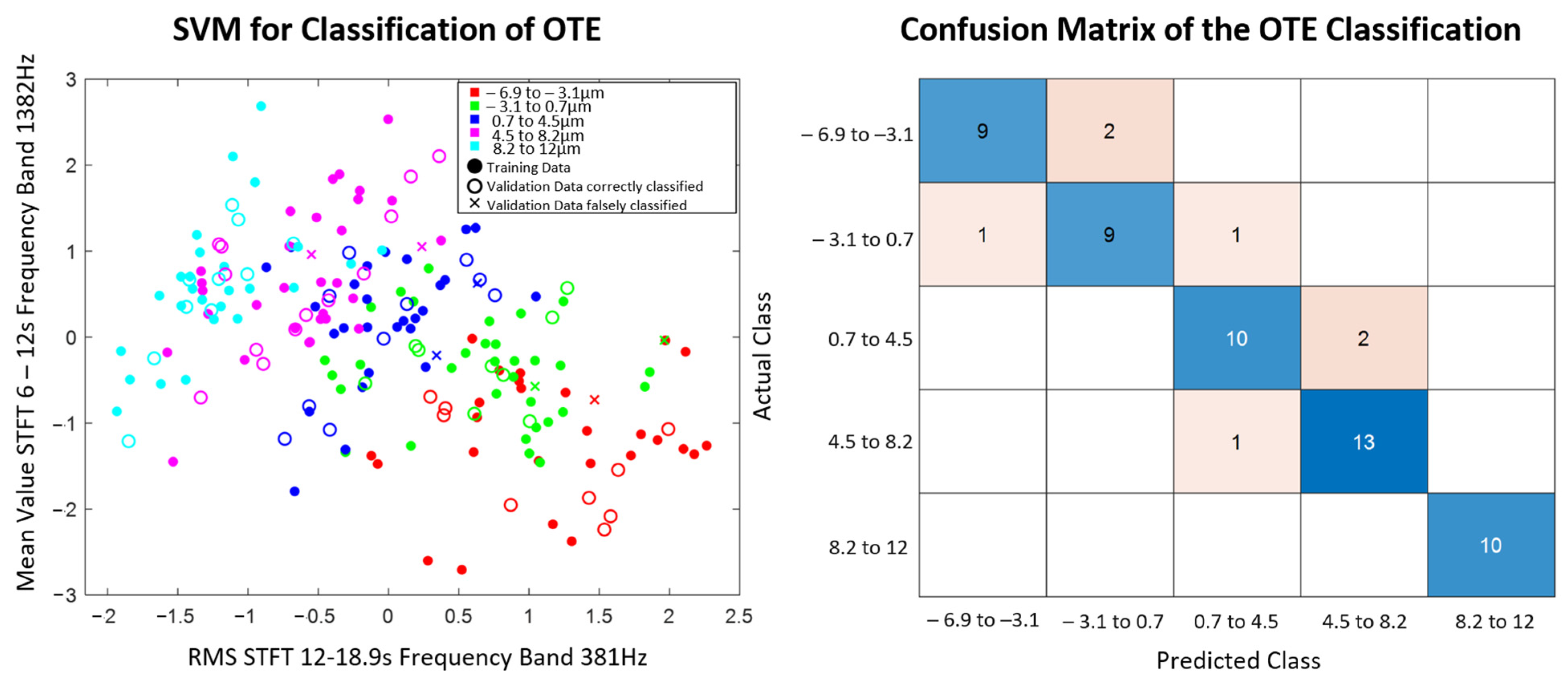
The SVM achieves the highest accuracy of 0.88 using the MANOVA selected features from the raw signal and the STFT. The highest-scoring two-way combination of the four selected features and the confusion matrix of the model are shown in Figure 13. When the trained model misclassifies data points, they are in adjacent classes to the true class. The KNN method, which uses a combination of features extracted from the raw signal, and the WPT, with 15 coefficients using ANOVA and the rank correlation coefficient, is the worst at predicting the OTE. It has an accuracy of 0.36 and assigns misclassified data points to distant classes.

5.3.4. Total Profile Deviation

The accuracy values of the classification of the profile total deviation with different classification methods and feature selections are shown in

Table 8. Evaluations of the classification models for the classification of the profile total deviation.

Feature Selection	Number of Features	Accuracy Bayes	Accuracy SVM	Accuracy KNN
MANOVA RS + STFT	2	0.76	0.76	0.76
MANOVA RS + CWT	2	0.81	0.76	0.72
MANOVA RS + DWT	2	0.71	0.76	0.72
MANOVA RS + WPT with 15 coeff.	2	0.71	0.76	0.67
MANOVA RS + WPT with 128 coeff.	2	0.67	0.76	0.67
ANOVA + rs RS + STFT	60	0.79	0.78	0.79
ANOVA + rs RS + CWT	60	0.71	0.72	0.76
ANOVA + rs RS + DWT	60	0.76	0.16	0.36
ANOVA + rs RS + WPT with 15 coeff.	60	0.67	0.72	0.78
ANOVA + rs RS + WPT with 128 coeff.	60	0.72	0.81	0.78

.

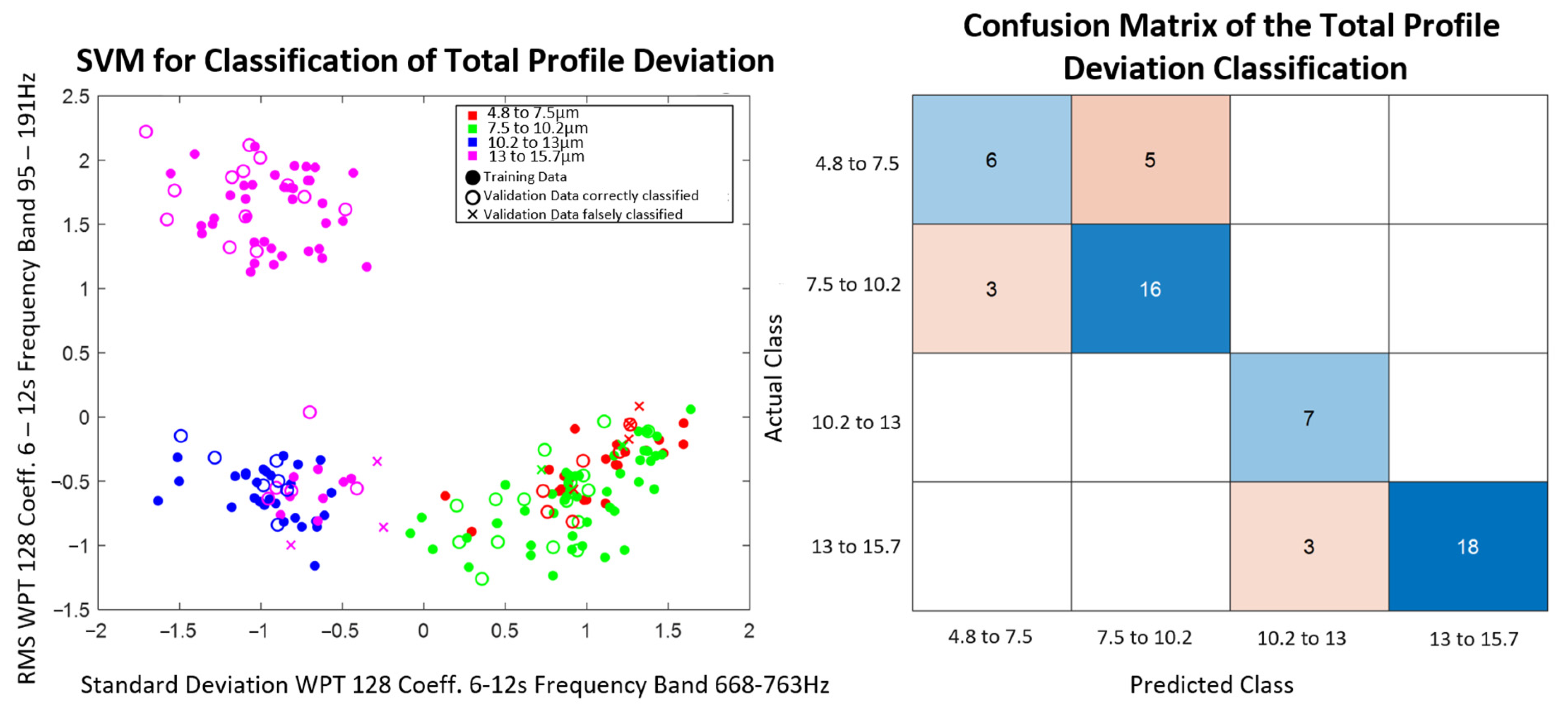
Both the SVM with features selected by ANOVA and the rank correlation coefficient from the raw signal and the WPT with 128 coefficients, and the Bayes classifier with features selected by MANOVA from the raw signal and the STFT, achieve the highest accuracy of 0.81. The SVM, with features selected by ANOVA and the rank correlation coefficient from the raw signal and the WPT with 128 coefficients, achieves the highest accuracy of 0.81. For the two best performing of the 60 features selected from the raw signal and the WPT, the training and validation data and the SVM confusion matrix are shown in Figure 14. The SVM that selects features from the raw signal and the DWT using ANOVA and the rank correlation coefficient is the worst suited for the classification of the profile total deviation. It misclassifies 84% of the data points with an accuracy of 0.16.

In general, the results have demonstrated that employing a support vector machine (SVM) leads to the minimum number of classification errors. However, the precision of classification predictions significantly relies on the chosen features, which are determined by the applied feature extraction and selection techniques, that should be tailored to the specific parameter of interest. For future research, we propose exploring smaller parameter ranges and additional influencing variables through a long-term experiment that should run parallel to the production process. This long-term experiment would enable investigating tool wear and significantly increase the size of the training data set. In this context, the use of neural networks is promising, which, in addition to a regression, also enables an image-based evaluation of the recorded acoustic signals in the frequency domain. There are already studies, on which to build on, which investigate the suitability of convolutional neural networks and deep belief network for the classification of faulty tool states by means of image-based acoustic data [37,38].

6. Conclusions

The focus of this study was to investigate the suitability of process-integrated structure-borne sound measurements for monitoring the hobbing process of microgears. The study aimed to use machine learning models to predict process parameters, such as radial feed and tool tumble, and evaluate quality characteristics, such as overall transmission error and total profile deviation. Additionally, a data processing chain was shown, from feature extraction to predicting the desired parameters. In this process, methods for feature selection and various classification algorithms were compared and evaluated. Overall, the results have shown that the use of an SVM generates the least classification errors. However, the prediction accuracy of the classification depends heavily on the features used, which are in turn determined by the applied feature extraction and selection. These are to be chosen according to the parameter of interest. Overall, at least 90% of the process parameters and at least 81% of the quality characteristics can be predicted correctly. Thus, it was shown that structure-borne sound in combination with machine learning and data analysis, was suitable for classifying process parameters as well as quality characteristics and hence enables economical, 100% inline measurements of microgears.

For future works, an investigation of smaller parameter ranges and additional influencing variables in a long-term experiment is proposed. Model augmentation could be a way to adjust the robustness of the model to changing conditions in the long-term test [39]. In addition, the approach may need to be adapted to include continuous trainability in order to constantly adapt to changing conditions (tool replacement or wear, environmental noise, etc.). This should be carried out in parallel to production in order to depict tool wear as well as to increase the size of the training data set considerably. The focus of future studies is on using regression models for a more accurate prediction of the process parameters and quality characteristics to enable the implementation of adaptive process control strategies.

References

1. Arndt, O.; Hennchen, S. Wertschöpfungs-und Wettbewerberanalyse für den Spitzencluster MicroTEC Südwest. Prognos AG Bremen Düsseldorf 2011, 8. [Google Scholar]
2. Slatter, R. Mikroantriebe fur prazise Positionieranwendungen. Antriebstechnik 2003, 42, 30–35. [Google Scholar]
3. VDI 2731: Microgears—Basic Principles Part 1; VDI Verein Deutscher Ingenieure e.V., Beuth: Berlin, Germany, 2009.
4. Klocke, F.; Brecher, C. Untersuchung von Zahnradgetrieben. In Zahnrad-und Getriebetechnik; Klocke, F., Brecher, C., Eds.; Carl Hanser Verlag GmbH & Co. KG: München, Germany, 2016; pp. 363–553. [Google Scholar]
5. Gravel, G. Bestimmung von Welligkeiten auf Zahnflanken. In Kongress zur Getriebeproduktion, Congress Centrum Würzburg; FVA GmbH: Frankfurt, Germany, 2009; pp. 11–12. [Google Scholar]
6. Härtig, F.; Hirsch, J.; Jusko, O.; Kniel, K.; Neuschaefer-Rube, U.; Wendt, K. Koordinatenmesstechnik als Schlüsseltechnologie der Fertigungsmesstechnik Coordinate Metrology as a Key Technology in Production Measurement. tm-Technisches Messen 2009, 76, 73–82. [Google Scholar] [CrossRef]
7. Galczyński, R. Effect of hob wear on the sounds emitted in the gear hobbing process. Precis. Eng. 1984, 6, 25–30. [Google Scholar] [CrossRef]
8. Li, Y.; Wang, X.; He, Y.; Wang, Y.; Wang, Y.; Wang, S. Deep Spatial-Temporal Feature Extraction and Lightweight Feature Fusion for Tool Condition Monitoring. IEEE Trans. Ind. Electron. 2022, 69, 7349–7359. [Google Scholar] [CrossRef]
9. Niehaus, F.; Peschke, C.; Weck, M.; Wenzel, C. Ultrapräzisionsmaschinen (ab 1988). In 100 Jahre Produktionstechni; Eversheim, W., Pfeifer, T., Weck, M., Eds.; Springer: Berlin/Heidelberg, Germany, 2006; pp. 541–555. [Google Scholar]
10. Ogedengbe, T.I.; Heinemann, R.; Hinduja, S. Feasibility of tool condition monitoring on micro-milling using current signals. AU JT 2011, 14, 161–172. [Google Scholar]
11. Zhu, K.; Vogel-Heuser, B. Sparse representation and its applications in micro-milling condition monitoring: Noise separation and tool condition monitoring. Int. J. Adv. Manuf. Technol. 2014, 70, 185–199. [Google Scholar] [CrossRef]
12. Prakash, M.; Kanthababu, M. In-Process Tool Condition Monitoring Using Acoustic Emission Sensor in Microendmilling. Mach. Sci. Technol. 2013, 17, 209–227. [Google Scholar] [CrossRef]
13. Su, L.Y. Micro-Vibration Mechanism of Micro-Gears Fault Diagnosis Based on Fault Characteristics and Differential Evolution Wavelet Neural Networks. AMM 2014, 508, 219–222. [Google Scholar] [CrossRef]
14. Möser, M.; Kropp, W. Körperschall; Springer: Berlin/Heidelberg, Germany, 2010. [Google Scholar]
15. Möser, M. Körperschall-Messtechnik; Springer: Berlin/Heidelberg, Germany, 2018. [Google Scholar]
16. Marinescu, I.; Axinte, D.A. A critical analysis of effectiveness of acoustic emission signals to detect tool and workpiece malfunctions in milling operations. Int. J. Machine Tools Manuf. 2008, 48, 1148–1160. [Google Scholar] [CrossRef]
17. König, W.; Kutzner, K.; Schehl, U. Tool monitoring of small drills with acoustic emission. Int. J. Machine Tools Manuf. 1992, 32, 487–493. [Google Scholar] [CrossRef]
18. Sturm, A.; Förster, R. Einführung in die Theorie der Technischen Diagnostik. In Maschinen-und Anlagendiagnostik; Springer: Berlin/Heidelberg, Germany, 1990; pp. 18–92. [Google Scholar]
19. Yum, J.; Kim, T.H.; Kannatey-Asibu, E. A two-step feature selection method for monitoring tool wear and its application to the coroning process. Int. J. Adv. Manuf. Technol. 2013, 64, 1355–1364. [Google Scholar] [CrossRef]
20. Maia, L.H.A.; Abrao, A.M.; Vasconcelos, W.L.; Sales, W.F.; Machado, A.R. A new approach for detection of wear mechanisms and determination of tool life in turning using acoustic emission. Tribol. Int. 2015, 92, 519–532. [Google Scholar] [CrossRef]
21. Papenfort, J.; Frank, U.; Strughold, S. Integration von IT in die Automatisierungstechnik. Informatik Spektrum 2015, 38, 199–210. [Google Scholar] [CrossRef]
22. Erkaya, S.; Ulus, Ş. An Experimental Study on Gear Diagnosis by Using Acoustic Emission Technique. IJAV 2016, 21, 103–111. [Google Scholar] [CrossRef]
23. Wang, B.; Liu, Z. Acoustic emission signal analysis during chip formation process in high speed machining of 7050-T7451 aluminum alloy and Inconel 718 superalloy. J. Manuf. Process. 2017, 27, 114–125. [Google Scholar] [CrossRef]
24. Inasaki, I. Application of acoustic emission sensor for monitoring machining processes. Ultrasonics 1998, 36, 273–281. [Google Scholar] [CrossRef]
25. Wantzen, K. Methode zur Entwicklung Merkmalsbasierter Zustandsüberwachungssysteme Mittels der Körperchallmesstechnik. Doctoral Dissertation, Karlsruher Institut für Technologie, Karlsruhe, Germany, 2020. [Google Scholar]
26. Motor & Gear Engineering Inc. Gear Hobbing: Introduction, Working, Advantages, and Applications. Available online: https://www.motorgearengineer.com/blog/gear-hobbing-introduction-working-advantages-applications/ (accessed on 6 February 2023).
27. Carrino, S.; Guerne, J.; Dreyer, J.; Ghorbel, H.; Schorderet, A.; Montavon, R. Machining quality prediction using acoustic sensors and machine learning. Proceedings 2020, 63, 31. [Google Scholar]
28. Klocke, F. Fertigungsverfahren 1; Springer: Berlin/Heidelberg, Germany, 2018. [Google Scholar]
29. Gauder, D.; Gölz, J.; Biehler, M.; Diener, M.; Lanza, G. Balancing the trade-off between measurement uncertainty and measurement time in optical metrology using design of experiments, meta-modelling and convex programming. CIRP J. Manuf. Sci. Technol. 2021, 35, 209–216. [Google Scholar] [CrossRef]
30. QASS. Analyzer4D Handbuch. Available online: https://www.qass.net/downloads/Handbuch_Analyzer4D_V1.7.1.pdf (accessed on 3 January 2023).
31. Bruker Alicona. Optische Koordinatenmessmaschine für Komplexe Geometrien. Available online: https://www.alicona.com/de/produkte/cmm/ (accessed on 3 January 2023).
32. Mikut, R. Data Mining in der Medizin und Medizintechnik; KIT Scientific Publishing: Karlsruhe, Germany, 2008. [Google Scholar]
33. ISO 1328-1:2013; Zylinderräder—ISO-Toleranzsystem: Teil 1: Definitionen und Zulässige Werte für Abweichungen an Zahnflanken. Beuth: Berlin, Germany, 2013.
34. Liu, M.-K.; Tseng, Y.-H.; Tran, M.-Q. Tool wear monitoring and prediction based on sound signal. Int. J. Adv. Manuf. Technol. 2019, 103, 3361–3373. [Google Scholar] [CrossRef]
35. Klocke, F.; Döbbeler, B.; Goetz, S.; Viek, T.D. Model-Based Online Tool Monitoring for Hobbing Processes. Procedia CIRP 2017, 58, 601–606. [Google Scholar] [CrossRef]
36. León, F.P.; Jäkel, H. Singale und Systeme; De Gruyter: Oldenburg, Germany, 2019. [Google Scholar]
37. Kale, A.P.; Wahul, R.M.; Patange, A.D.; Soman, R.; Ostachowicz, W. Development of Deep Belief Network for Tool Faults Recognition. Sensors 2023, 23, 1872. [Google Scholar] [CrossRef] [PubMed]
38. Patil, S.S.; Pardeshi, S.S.; Patange, A.D. Health Monitoring of Milling Tool Inserts Using CNN Architectures Trained by Vibration Spectrograms. Comput. Model. Eng. Sci. 2023, 136, 177–199. [Google Scholar] [CrossRef]
39. Patange, A.D.; Pardeshi, S.S.; Jegadeeshwaran, R.; Zarkar, A.; Verma, K. Augmentation of Decision Tree Model Through Hyper-Parameters Tuning for Monitoring of Cutting Tool Faults Based on Vibration Signatures. J. Vib. Eng. Technol. 2022, 1–19. [Google Scholar] [CrossRef]
Figure 2. Sensor integration in the machine (image source: [26].)
Algorithms 16 00183 g002
Figure 3. CAD layout of the sensor integration (sensor in blue on the left, sensor with protecting housing on the right).
Algorithms 16 00183 g003
Figure 4. Sensor integration in the machine.
Algorithms 16 00183 g004
Figure 5. Data acquisition and analysis workflow [30,31].
Algorithms 16 00183 g005
Figure 6. Classification data pipleine.
Algorithms 16 00183 g006
Figure 7. Visualization of the overall transmission error (OTE).
Algorithms 16 00183 g007
Figure 8. Raw signal with a tumble of 0 µm and a radial feed of 0 mm as well as overview of the time intervals used and the process steps of the hobbing process.
Algorithms 16 00183 g008
Figure 9. Comparison of the spectra of the hobbing process with cutter contact (left) and without contact (right).
Algorithms 16 00183 g009
Figure 10. STFT spectra at different radial feeds and a tool tumble of 0 µm.
Algorithms 16 00183 g010
Figure 11. Best two features and confusion matrix of SVM for radial-feed classification (feature selection: MANOVA, features from raw signal and WPT with 15 coefficients).
Algorithms 16 00183 g011
Figure 12. Best two features and confusion matrix for tool tumble classification (feature selection: ANOVA+rs from raw signal and STFT).
Algorithms 16 00183 g012
Figure 13. Best two features and confusion matrix of SVM to classify the OTE (feature selection: MANOVA, features from raw signal, and STFT).
Algorithms 16 00183 g013
Figure 14. Best two features and confusion matrix of SVM for classification of profile total deviation (feature selection: ANOVA+rs, features from raw signal and WPT with 128 coefficients).
Algorithms 16 00183 g014