Abstract
The time-dependent diffusion equation is studied, where the diffusion coefficient itself depends simultaneously on space and time. First, a family of novel, nontrivial analytical solutions is constructed in one space dimension with the classical self-similar Ansatz. Then, the analytical solution for two different sets of parameters is reproduced by 18 explicit numerical methods. Fourteen of these time integrators are recent unconditionally stable algorithms, which are often much more efficient than the mainstream explicit methods. Finally, the adaptive time-step version of some of these algorithms are created and tested versus widespread algorithms, such as the Runge–Kutta–Fehlberg solver.
1. Introduction
Regular diffusion or regular heat conduction in solid media are among the simplest transport processes, which can be described by a single linear partial differential equation (PDE) of space and time. Diffusion means the transport of particles, while heat conduction means the transport of energy. If , and the unknown function (temperature in the case of heat conduction and concentration in the case of particle diffusion) is denoted by , then the simplest regular diffusion PDE in one space dimension is
where is usually a given function and is the constant diffusion coefficient. In the case of heat conduction, is the thermal diffusivity, while c, ρ, and k are the specific heat, the density, and the heat conductivity of the material, respectively. The boundary conditions will be discussed in the concrete analytical and numerical examples.
It is clear that for the regular diffusion equation, some analytical solutions exist [1,2], which can be found in basic textbooks. These solutions have crucial relevance to understanding the diffusion process itself. As a second point, these solutions help to test the properties and performance of old and new numerical methods. Unfortunately, in numerous engineering problems, the properties of the materials, such as the density, diffusivity, heat conductivity, or specific heat, can widely vary in the system [3] due to natural or artificial inhomogeneities; therefore, the diffusion coefficients should also have some kind of spatial and/or temporal dependence.
The Fick–Jacobs equation [2] (p. 68)—which is the most general space-dependent diffusion equation—can be directly derived based on the Fokker–Planck equation. The proper derivations were performed by Reguera and Rubi [4] and by Zwanzig [5]. Using these equations, one can describe single-particle diffusion processes in systems which have spatial inhomogeneities, such as narrow ribbon channels [6]. Such systems are created when molecules diffuse through carbon nanotubes [7], systems of channels like in zeolites [8], or even in cell membranes [9]. Diffusion equations with space-dependent and time-dependent coefficients were also used to model the movement of molecular species in water by Amiri at al. [10] and Hefny and Tawfik [11], respectively.
Previously, we investigated the regular and irregular diffusion equations [12,13]. For the regular diffusion equation (such as Equation (1)) with the traveling wave, self-similar, traveling profile, or with some generalized self-similar trial functions, numerous new types of analytic solutions were found. These solutions have a much more complicated structure than the well-known Gaussian (plus an error function in the most general case). Our new formulas contain Kummer’s or Whittaker functions with quadratic arguments with a new free parameter which results in a larger variety of solutions. These solutions can have a drastically different rate of decay than the fundamental Gaussians. We found solutions which have some oscillatory behavior with a rapid power-law decay both in space and time.
In this work, we modify the PDE (1) to have a diffusion coefficient which is non-constant in two senses. We introduce a new variable, which is a combination of the space and time variable: . The diffusion coefficient has the simplest power-law dependence on this variable: , where D is a constant, whose physical dimension depends on the concrete value of β and m. Inserting it into the diffusion equation, we obtain
Equations (1) and (2), and similar kinds of equations, are most frequently solved numerically [14], and several methods are proposed for this purpose. Most of them can be classified as either explicit or implicit schemes. Both kinds have a major advantage and a disadvantage compared to one another. The widely used explicit methods, such as the FTCS (forward time central space), require a fairly short time to execute a time step and they are easily parallelizable. However, they are unstable, and the solution is expected to blow up if the time-step size exceeds the so-called CFL (Courant–Friedrichs–Lewy) limit. In other words, their stability region is limited [15]. In our case, due to the space dependence of the diffusion coefficient, this limit is rather small, and the stiffness ratio is high. On the other hand, due to the time dependence of the coefficient, it is changing in time, so using the traditional explicit methods is very risky.
The stability of the implicit methods is fundamentally better; therefore, they are considered superior and commonly used by many scientists to solve these and similar equations [16,17,18]. However, in each time step, it is required to solve a system of algebraic equations for which the process is not easily parallelizable. Calculations can be very slow with large amounts of memory. This is common in multiple dimensions of space when the matrix has a huge size and is non-tridiagonal. Moreover, with implicit methods, it is much harder to follow the trend toward increasing parallelization. So, it is shown that explicit methods can be more efficient even if a small time-step size has to be applied [19]. It is worth noting that many clever combinations of the explicit and the implicit approaches, e.g., semi-explicit or semi-implicit methods, are also proposed [20,21,22,23]. Nevertheless, they do not resolve the above-mentioned dilemma of the explicit and implicit methods.
Regarding the above information, it is not baseless to believe that explicit methods, especially if they have enhanced stability properties (see [24,25,26,27,28,29,30,31] for examples), have an increasing comparative advantage over the long term. A couple of years ago, we initiated the development of new explicit methods, which are unconditionally stable, at least for the linear diffusion or diffusion–reaction equation. Our original publications (see, e.g., [32,33,34]) investigated the new methods theoretically and tested them with simple analytical as well as with numerical reference solutions. We have shown that they can provide quite accurate results significantly faster than the widely used methods, including MATLAB ODE solvers. In [35], we tested 14 methods in the case of a space-dependent diffusion coefficient. Most of these algorithms had been proposed by us previously as explicit and stable schemes, but we also included Dufort–Frankel and other known methods. However, as far as we know, until now no one tested any of these algorithms when the diffusion coefficient was both space and time dependent. Moreover, we do not know any work in which unconditionally stable explicit methods with an order larger than one are used to construct adaptive time-step size solvers.
The rest of this work is organized as follows. In Section 2, we analytically solve the investigated equations and present the results. Section 3 describes the discretization procedure and the numerical schemes used. In Section 4, the tests are performed for two sets of parameters to see how the methods perform in different situations. Then, in Section 5, the LNe-type methods are organized into adaptive time-step size solvers and tested against popular Runge–Kutta solvers. Finally, in Section 6, we summarize our conclusions and mention future research directions.
2. Analytical Solution
To solve the PDE (2), we use the well-known reduction technique, where we define a new variable , which is a combination of the spatial and temporal variable. Then, we try to find the solution with the self-similar Ansatz in the form of , where α and β are arbitrary real constants, and is the shape function with existing first and second continuous derivatives with respect to η. Evaluating the first temporal and second spatial derivative of this Ansatz and substituting these back to the PDE (2) yields
where prime means derivation in respect to the reduced variable η. To complete the reduction mechanism, the explicit presence of the time variable has to be eliminated. From this requirement, we arrive at the following constraints for the parameters, α = arbitrary real number, , while m remains an arbitrary real parameter. Now, we have the ordinary differential equation (ODE) for
where and are the Whittaker functions [36,37]. There is a connection to the former results, which can be seen if one checks the following formulas which express the Whittaker functions [36] in terms of the Kummer functions M and U:
Due to the exponential factor in Equation (5), the Whittaker functions have a quicker decay than the Kummer functions. The shape functions for some parameter values are presented in Figure 1. The time development of the function u for two given parameter sets are shown in Figure 2 and Figure 3. It can be shown with a careful parameter analysis that for negative values of α, the solutions have an exponential growth at large time and spatial coordinates which may be considered non-physical; thus, we exclude them from further numerical investigations. Diffusion processes where the concentration or the number of particles explodes violate energy and matter conservation laws. On the other hand, for some values of the parameters and variables, the values of u can be complex, which may be considered non-physical. We also note that because our analytical solution is valid on the whole real axis, the boundary conditions need to be specified only when the analytical solution is going to be reproduced by numerical methods.
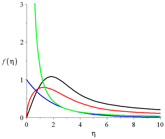
Figure 1.
The solution of Equation (3) with D = 1; ; c1 = 1; c2 = 0: the black, red, blue, and green lines are for (m = 0; 1/2; 1; 5/2).
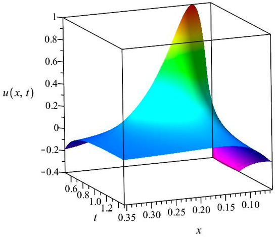
Figure 2.
The solution of Equation (2) with the shape function Equation (4) for .
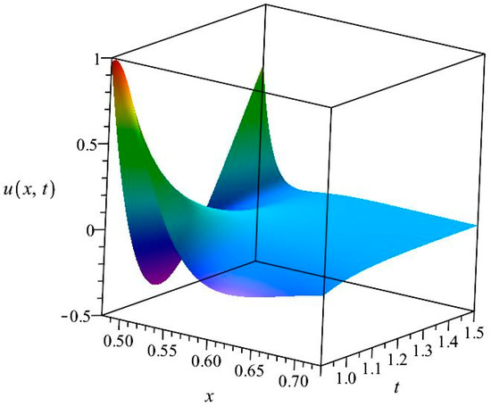
Figure 3.
The solution of Equation (2) with the shape function Equation (4) for .
In our numerical experiments, we always choose and set the value of to be a normalization constant. It means that we are going to numerically reproduce the following reference solution:
In Figure 2 and Figure 3, we present 3D plots of this u function for those two cases, which will be reproduced numerically in the latter sections. Note that in the second case, the u function on the left boundary is first decreasing from positive to negative values and then increasing to reach positive values again; the numerical methods should follow this nontrivial behavior.
3. The Procedure of the Numerical Solution
3.1. The Spatial and Temporal Discretization
We consider the case of heat conduction because the concepts of the following discretization process are better established in this case. Let us discretize the time variable uniformly, which means , and
On the interval , we construct an equidistant spatial grid:
The parameters , , etc., will be given when the concrete examples are presented.
If the physical properties of the heat-conducting media depend on space, the following PDE is used:
For simplicity, we consider and in this work, and all the space and time dependence of the diffusivity will be incorporated into the conductivity . When the outer differentiation with respect to x is executed at the right-hand side of (7), the term must also be differentiated, which implies that an extra drift term with appears, such as in Equation (2). We avoid this by discretizing the function k and simultaneously in Equation (7). The usual central difference formula is employed to obtain
We now move from node variables to cell variables. It means that is the approximation of the average temperature of cell i, by its value at the cell center. Furthermore, is the heat conductivity between cell i and its (right) neighbor, estimated by its value at the border of the cells. Now, the previous formula will have the form
Because we are in one spatial dimension, we consider the cross-section area of the system as unity. Now, the heat capacity of the cell is the same as the volume and can be given as . The thermal resistances at the n-th time level are calculated as follows:
Now, we have the equation for the time derivative of each cell variable:
which can be written into a matrix form
where the system matrix M is dimensional and depends on the time variable. More details about this way of discretization (for the case of the time-independent case but more space dimensions) can be found, e.g., in [33].
The numerical methods examined in this work can be used in the case of different types of boundary conditions, e.g., Dirichlet, Neumann, and periodic. Because we reproduce the above given analytical solutions, we always use Dirichlet boundary conditions, but the concrete details will be given later.
3.2. The Applied 18 Numerical Algorithms
All the 18 numerical algorithms are already known. However, all of them (except perhaps the RK4) are generalized to the case of a space- and time-dependent diffusion coefficient for the first time here. Let us present immediately the formulas which are applied for Equation (8) or (9), as well as the references where the readers can find more details about them. We note that 14 of the used formulas are collected and applied in our previous paper [35] for the case when D depends only on space but not on time. The following two quantities will be extensively used:
The quantity is similar to the mesh ratio , which is usually used in the case of Equation (1). The quantity will convey information to the cell i from its neighbors. We will frequently employ the modified theta-formula:
which is thoroughly introduced and described in [38].
1. The so-called unconditionally positive finite difference (UPFD) method is developed by Chen-Charpentier and Kojouharov [39] for the linear diffusion–advection–reaction equation. In our case, the new values of the cell variables can be obtained from Equation (10) by the substitution:
2. The simplest among our methods is the constant neighbor (CNe) algorithm [32]. The following formula is used:
3. The two-stage CpC method [40] uses the CNe formula twice. The first stage is a fractional time step with length h/2, where the new predictor values of u are calculated as follows:
Note that in the second term on the r. h. s., the factor ½ cancels out from the fraction. The new values of the A quantities are calculated using these predictor values
and then, at the second stage, these are used in the full-length corrector step. The function values at the end of the time step are
Note that the resistances are taken into account only at the beginning of the time step, and they are updated only when a new time step begins. This tactic will be used in the case of the next methods, which are based on the so-called linear-neighbor approximation.
4. The linear-neighbor (LNe or LNe2) algorithm [32] consists of two stages. The first stage is actually a full predictor time step with the CNe scheme to calculate the values. Using them, we can calculate new values:
Now, the corrector step uses the following formula:
5–6. Based on the corrector values in Equation (15), one can first recalculate again, and then repeat (15) to obtain new corrector values. This three-stage scheme is called the LNe3 method [32], which is still second order, but it is usually more accurate than the LNe2. If one repeats the corrector step again based on the LNe3 values to further improve the accuracy, a four-stage formula arises, which is abbreviated as LNe4.
7. The CLL algorithm [41] is a modification of the LNe3 algorithm in order to achieve third-order temporal convergence. For this purpose, it uses fractional time steps during the first and second stages. Generally, the length at the first stage is , , but at the second stage it is always . In the first stage, the CNe formula is employed to calculate new predictor values:
In the second stage, we use formulas similar to (15) but with an time-step size to obtain the first corrector values. The new values are calculated as in Equation (14), i.e., . Using these the corrector step is as follows:
In the third stage, a full time step is taken with the LNe formula:
where . In Section 4, we take , but in Section 5 we try p = 1 as well.
8. The CCL algorithm [42] is very similar to the CLL, but at the second stage the CNe formula is used. So, the first stage is the same as in (16), where, for stability reasons, and should hold. We set and obtain the first- and second-stage formulas:
Then, after the calculation of , a full time step is taken with the LNe formula at the third stage:
9. The two-stage pseudo-implicit (PI) method is published in [38]. It is considered here with parameters and at the first stage and at the second stage. The following first- and second-stage formulas must be applied for each cell:
where is calculated exactly as in Equation (13). One can see that there is a stage with a half time step for the predictor values and then the second stage with a full time step for the corrector values.
Let us now focus on the odd–even hopscotch schemes. A bipartite spatial grid, in which all the nearest neighbors of the odd cells are even and vice versa, is required to apply any of them. There are four different stencils, more precisely spatial and temporal structures, of the used hopscotch-type methods, which are displayed in Figure 4. Only one odd and one even cell is displayed in the case of each method in the figure. The stages are symbolized by colored rectangles. Those boxes which belong to the repeating units are surrounded by dashed red lines. For example, the asymmetric hopscotch structure (ASH) consists of two half and one full time steps. The calculation starts with a half-sized time step (yellow rectangle with the number ‘1’ inside) being taken for the odd cells using the initial values. Then, a full time step is taken for the even cells (green box), and then a halved third timestep (blue rectangle) closes the repeating unit of the calculation, which is surrounded by a dashed red line. The golden rule is that the most recent values of the neighbors always have to be used when an is calculated (for example, in the theta-formula) to obtain the new value of ui. This assures stability and, at the same time, quite quick convergence. At the next points, we give the concrete formulas with which the structures can be filled. In the case of the theta-formula, we just give the value of the parameter θ.
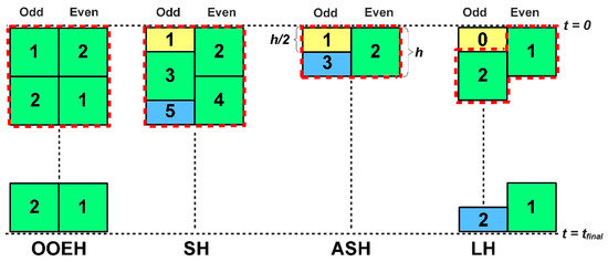
Figure 4.
Hopscotch-type space-time structures. The time elapses from the top (t = 0) to the bottom.
10. Original odd–even hopscotch method (OOEH, [43]): Stage 1: , Stage 2: .
11. Reversed odd–even hopscotch algorithm (RH, [34]), uses the same structure as the OOEH. Stage 1: , Stage 2: .
12. OEH-CNe method: OOEH structure, CNe formula in each stage with the golden rule mentioned above.
13. Shifted-hopscotch (SH, [33]): Stage 1 (yellow box in Figure 4): , Stages 2–4 (green boxes): , Stage 5 (blue box): .
14. Asymmetric-hopscotch (ASH, [44]): Stage 1 (yellow box), , Stage 2: , Stage 3: .
15. Leapfrog-hopscotch (LH, [45]): Stage 0 (yellow box): . Intermediate and last stages (green and blue boxes): .
16. Leapfrog-hopscotch-CNe (LH-CNe, [45]): CNe formula at all stages with the appropriate time-step size.
17. The Dufort–Frankel (DF) explicit two-step method [46] (p. 313) is an old but non-traditional algorithm which was constructed for the diffusion equation for which it is unconditionally stable. In our case, it has the formula:
The r. h. s. of the formula contain values of u at two time levels, so we need two initial conditions, the second one calculated by another algorithm. We employ the UPFD Scheme (11) for this purpose.
18. For comparison purposes, we use the so-called classical version of the fourth-order Runge–Kutta (RK4) method [47] (p. 737). If we apply it to our spatially discretized system, we have
and finally
With the exception of the UPFD, OOEH, DF, and RK4, all the methods were created by our research group. The verifications and almost always the analytical proofs are presented in the original papers, but several truncation errors are given in [48]. The UPFD and the CNe methods have been shown to have first-order convergence in the time-step size, CCL and CLL are third order, RK4 is obviously fourth order, and all other schemes are second order. All methods (except RK4, of course) are unconditionally stable for the linear heat or diffusion equation. This means that the CFL restrictions do not apply in their case. We underline once again that in the big camp of explicit methods, unconditional stability is not the rule but the exception.
Note that the CNe, CpC, LNe, LNe3, LNe4, OOEH-CNe, and LH-CNe schemes are not simply stable, but their error is strictly limited by the maximum and minimum principles [49] (p. 87). This is a direct consequence of the fact that any new value is the convex combination of the already known , etc., values, which excludes the increase in any unphysical oscillations even for extremely large time-step sizes. On the other hand, as the reader will see later, this favorable property limits the speed of convergence of these algorithms, often resulting in rather poor accuracies for small and medium time-step sizes. Specifically, they significantly (in the case of very large time-step sizes, tremendously) underestimate the speed of the heat- or particle-transfer process, which can be perceived as a kind of ‘negative’ dissipation error.
4. Numerical Results with Fixed Time-Step Sizes
This section investigates the numerical error, for example, how it decreases with the time-step size h. First, we run the simulation for all 18 methods for a very large and fixed h and calculate the error. Then, this procedure is repeated with smaller and smaller time-step sizes until the minimal error values are obtained. The magnitude of the error is calculated as follows:
which means the usual error, i.e., the largest absolute difference between the analytical and the numerical solution at the final time , is considered. Because some data about the running times of the examined methods for fixed time-step sizes can be found in our original publications, we do not measure the running times here, only in Section 5 with adaptive time-step sizes.
The system matrix M has only negative eigenvalues. Let us denote the smallest (largest) absolute value eigenvalues by . The CFL limit for the explicit Euler method can be analytically calculated as , and for the higher-order RK method, this limit is only slightly larger [50]. On the other hand, the stiffness ratio of the problem can be defined as the ratio .
To perform the numerical calculations, the software MATLAB has been used, and the command kummerU has been used to calculate the Kummer U function (confluent hypergeometric function of the second kind). Because the calculation of the values of the boundary conditions for a given time point is orders of magnitude more time-consuming than performing the steps of the numerical schemes for all the nodes of the grid, we applied a trick to minimize the running time. The boundary conditions have been calculated only in 4000 time points, and a linear interpolation between the two appropriate times of the pre-calculated boundary values has been used to evaluate the boundary conditions at the actual time of the simulation. Of course, we always checked that the error due to this approximation is always much smaller than the errors of the numerical algorithms at the intermediate space points.
4.1. Experiment 1 with Small Value of Parameter m
In this experiment, the following parameters are used:
The CFL limit is increasing from to and the stiffness ratio is decreasing from to . The errors as a function of the time-step size are presented in a log-log diagram in Figure 5. The errors cannot decrease below the residual error (from space discretization), which is visible in the bottom left of the figure, because we employ a fixed space step size and only reduce the time-step size. The RK4 method is unstable for large and medium time-step sizes, and therefore it is visible only at the bottom left side of the figure. Two groups of the stable methods are clearly distinguishable: the slowly and the quickly converging algorithms. This latter one consists of the OOEH, RH, SH, ASH, DF, and LH methods, and the remaining 11 converge more slowly. In our paper [48], we explained the reasons for this behavior based on the truncation errors. Note that a slowly converging algorithm does not mean that it is useless, because it can possess other useful properties, such as the previously mentioned minimum–maximum principle.
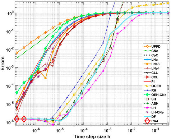
Figure 5.
Maximum errors as a function of the time-step size for Experiment 1. The numerical order of convergence of the algorithms are the slopes of the error curves.
In Figure 6, one can see the analytical u function at the initial and final time, as well as the numerical solution at the final time in the case of two methods, namely the CCL and the LH methods, for those time-step sizes when they start to produce a solution which may be acceptable in some engineering applications. Moreover, in Figure 7, we also plotted the time development of the maximum errors of all but the RK4 schemes for a fixed time-step size .
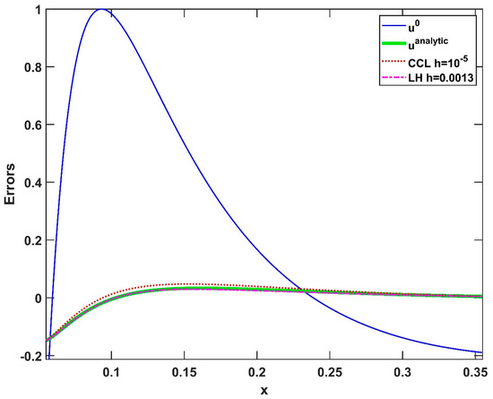
Figure 6.
The variable u as a function of x in the case of the initial function u0, the analytical solution at the final time, the CCL algorithm for , and the LH algorithm for in the case of small value of m (Experiment 1). It is worth emphasizing again that for these time-step sizes, explicit Runge–Kutta algorithms are unstable.
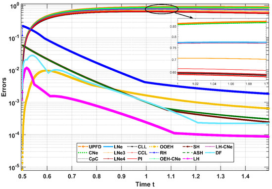
Figure 7.
The time development of the errors, i.e., the absolute difference between the analytical solution and that of the stable numerical methods, for as a function of time.
4.2. Experiment 2 with Large Value of Parameter m
In this experiment, the following parameters are used:
Because the value of m is larger, the diffusion coefficient depends on the x and t variables more strongly. The CFL limit is increasing from to and the stiffness ratio is decreasing from to . The errors as a function of the time-step size are presented in a log-log diagram in Figure 8. In Figure 9, one can see the analytical u function at the initial and final time, as well as the numerical solution at the final time in the case of the CCL and the LH methods. In Figure 10, we again plotted the time development of the maximum errors of all but the RK4 schemes for a fixed time-step size .
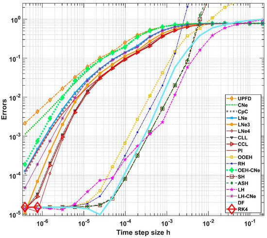
Figure 8.
Maximum errors as a function of the time-step size for parameter set (20) (Experiment 2).
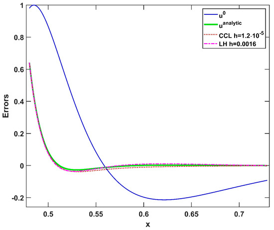
Figure 9.
The variable u as a function of x in the case of the initial function u0, the analytical solution at the final time, the CCL algorithm for , and the LH algorithm for in the case of large value of m (Experiment 2).
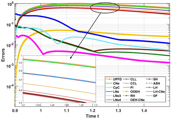
Figure 10.
The time development of the errors, i.e., the absolute difference between the analytical solution and that of the stable numerical methods, for as a function of time.
5. Numerical Results with Adaptive Time-Step Sizes
In this section, we introduce and design several adaptive time-step controllers to solve the system in Equation (8). When adaptive step-size controllers are designed, there are three important factors: the method for advancing the solution in each time step, the approach of estimating the local error in each time step, and the strategy which changes the size of the time step [51]. For advancing the solution, three methods have been used here to design the controllers, which are the LNe3, CLL, and Runge–Kutta methods. For estimating the local error, one needs the values of the function u calculated in two different ways but at the same time level. However, most of the examined algorithms do not automatically serve two different approximations of the unknown function. The LNe3 and the CLL methods are among those very few which do, so embedded formulas can be designed based on them, as will be explained for each method later.
The strategy for changing the time-step size can be briefly explained here. Let us assume that we applied an explicit scheme of order q with time-step size to the system in Equation (8) for advancing the solution from to . Assume that we used some approach for estimating the local error during that time step and let us denote the calculated local error by LE. The norm of the error estimation can be written as follows [52] (p. 26):
where AbsTol and RelTol are the relative and the absolute tolerances which can be specified by the user. The used nomenclatures hide the fact that LE and are vectors because they are applied to a system of ODEs instead of a single ODE. Using the calculated norm , we can change the time-step size using the following formula [53]:
where is a function of the norm of the error estimation , and that function depends on the type of the controller. The safety factor is taken as while the factors and are chosen to be and , respectively [54] (p. 168). In the case of the elementary controller, which we are using in this paper, the function can be written as follows:
If , we accept the time step, and the solution is advanced with , and the time step will be modified by Equation (22). If , we reject both the time step and the solution , and we repeat the calculations with a new time step calculated again by Equation (22).
Now, we will illustrate the approaches for calculating the local error estimation for each method.
The LNe3 method
As we introduced in Section 3, the LNe3 method consists of three stages. In the first stage, we use the CNe scheme while the LNe scheme is used in the second and third stages. All three stages provide values of the unknown function u at the end of the actual time step. It means that there are three possibilities to compare these values with one another in order to estimate the local error. The first possibility means that the difference between the numerical solutions calculated in the first and second stages is used as a local error estimator as follows:
where and are the solutions calculated by Equations (12) and (15), respectively. The indices C1 and L2 in the last nomenclature refer to the stages used to estimate the local error. Now, we substitute and into Equation (21) to obtain the norm of the local error estimation. Considering the previous calculations and Equations (22) and (23), an adaptive time-step controller is constructed, and it is denoted by ALNe3-C1L2. The local error can be estimated based on the first and third stages as well. Repeating the same step as in the previous lines, another adaptive time-step controller is obtained, and it is denoted by ALNe3-C1L3. The third possibility is when the local error is estimated based on the first and the third stages and the applied controller will be denoted by ALNe3-L2L3.
The CLL method
The CLL method consists of three stages. The first stage uses the CNe scheme with time-step length , while the second step uses the LNe scheme with time-step length . If we take in the first stage, then an error estimation can be made as in Equation (24), where is calculated by Equation (16), considering that , while is calculated by Equation (17). Substituting Equation (24) into Equation (21), and then considering Equations (22) and (23), an adaptive controller can be implemented, and it will be denoted by ACLL-C1L2. If , another local error estimation can be considered as follows:
where is calculated by Equation (16), taking , while is calculated by Equation (18). Substituting Equation (25) into Equation (21), and then considering Equations (22) and (23), an adaptive controller will be implemented, and it will be denoted by ACLL-C1L3.
Runge–Kutta Cash–Karp Method RKCK
Because it is a well-known method, and explained in detail in [55] (p. 717), we think that it is not necessary to describe the tedious processes of implementing the method. The local error estimation in Equation (16.2.6) and the fourth-order solution in Equation (16.2.5) in [55] can be plugged into our equation (21) to obtain the norm of the local error estimation. Again, using Equations (22) and (23), the Runge–Kutta Cash–Karp is obtained, and it is denoted by RKCK.
Runge–Kutta–Fehlberg Method
Plenty of references discussed and implemented this method. Here, we will refer to [56], where the authors show how to estimate the local error using Equation (5.55) in that reference. The numerical solution generated by Equation (5.53), along with the local error estimated by Equation (5.55) in that reference, can be substituted into our Equation (21) to obtain the norm of the error estimation. That norm can be used to adapt the time-step size using Equation (22), resulting in the so-called Runge–Kutta–Fehlberg 4(5), or RKF45 method, and it will be referred to as RKF in our paper.
Two numerical experiments are conducted to check the performance of these adaptive controllers and to compare their performances. The numerical computations are carried out using the MATLAB R2020b software on a desktop computer Intel Core (TM) i11-11700F.
5.1. Experiment 1 with Adaptive Solvers
In this experiment, the parameters listed in Equation (19) are used. The errors as a function of the running time are presented in a log-log diagram in Figure 11. From the figure, it is evident that the adaptive LNe3 controllers and the adaptive CLL controllers are significantly faster than the RKF and RKCK when the desired accuracy is not very high. The RKF and RKCK can achieve the same accuracy as the adaptive LNe and the adaptive CLL families with the same running time, only when the error is . However, none of the adaptive controllers can go beyond this accuracy due to the space discretization error. It does indeed look like the error, in the case of the RKF and RKCK, is relatively independent of the running time. According to our previous experience, this is not uncommon behavior in the case of explicit adaptive solvers, if the method used for designing the controller is only conditionally stable, such as some of the built-in ODE solvers of MATLAB [45].
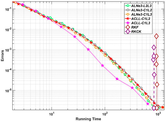
Figure 11.
The errors as a function of the running times in Experiment 1.
5.2. Experiment 2 with Adaptive Solvers
In this experiment, the parameters listed in Equation (20) are used. Figure 12 shows the errors as a function of the running time in a log-log diagram. This experiment shows that the adaptive LNe controllers and the adaptive CNe controllers are again faster than controllers designed based on the Runge–Kutta method. As we mentioned previously, the CFL limit is changing with respect to time, and it can be calculated for the explicit Euler method as . That limit was calculated in this experiment at six selected points in time as follows:
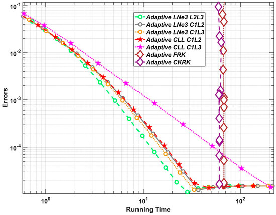
Figure 12.
The errors as a function of the running times in Experiment 2.
We plotted this limit as a function of time with a dashed blue line in Figure 13. At approximately the same level of accuracy, when the produced error was of order , the history of the time-step size was also registered for each adaptive controller in order to check if they can follow the trend of the . Figure 13 shows that the LNe3 controllers and CLL controllers could roughly follow the trend of the CFL limit. It means that they could detect the changes in the CFL limit and modify the step size. The Runge–Kutta controllers could follow the general trend, but they suffer from a fluctuating step size. The zoomed area of Figure 13 shows the behavior of the time-step size of the RKCK during a very short time (0.06% of the total time). On other hand, the time-step size in the case of the adaptive LNe3-L2L3 remained roughly constant. The reason behind the fluctuation in the case of the RK solvers is the conditional stability: when the time-step size h is below the CFL limit (which is slightly larger for RK4 than for the first-order explicit Euler), the error is very small, and the time-step size is increased. When the time-step size exceeds the stability limit, errors are starting to be amplified exponentially. This exponential increase can be very slow at the beginning if h is still close to the limit, which may yield a further time-step size elevation. Once the increasing error is detected, h is suddenly decreased to let the errors diffuse away. Then, the errors will be very small again; thus, the cycle starts again. This fluctuation is time-consuming and therefore undesirable. It is among the reasons why adaptive Runge–Kutta controllers are slower than the other solvers in our experiments.
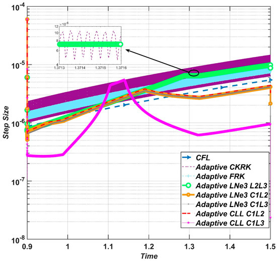
Figure 13.
The time-step size as a function time for the examined solvers.
6. Discussion and Summary
We studied the non-steady-state linear diffusion equation in the situation when the diffusion coefficient varies on the spatial and temporal coordinate at the same time. We have created a family of new analytical solutions using a similarity transformation, which is highly nontrivial, because the solution function is a combination of the two Whittaker functions.
A total of 18 explicit numerical algorithms have been used to reproduce this new analytical solution. Of them, 17 are explicit and unconditionally stable schemes which are recently invented, with the exception of 3 methods. The last one is the classical 4th-order Runge–Kutta method, which is only conditionally stable, and therefore it cannot be used with most of the time-step sizes applied in our experiments. According to our findings, the leapfrog-hopscotch scheme usually has the best performance, but the Dufort–Frankel, the original odd–even hopscotch, and the shifted and the asymmetric hopscotch can also be very accurate for much larger time-step sizes than the stability limit for the RK4 method. On the other hand, the LNe3 or LNe4 method is recommended if unconditional positivity is required. The LNe3 and the CLL algorithms have been successfully organized into embedded-type adaptive step size solvers, which severely outperform the standard RKF and RKCK solvers. Recall that a lot of efforts have been made to improve traditional solvers by the so-called PI and PID controllers [57,58]. The main goal of those controllers is to reduce the fluctuating behavior of the time-step size. The LNe3 and the CLL-based adaptive controllers could change the time-step size smoothly using only the elementary controller without any need to implement the PI controller. We consider this as another advantage of these methods. We can state that if the CFL limit is decreasing, the advantage of all the unconditionally stable explicit algorithms are increasing, and they can give results with acceptable accuracy much faster than the standard explicit methods. Therefore, we advise academics and engineers who still use the explicit RK solvers to solve linear diffusion or heat conduction equations to shift to an explicit but stable method.
In the near future, we are turning our attention to nonlinear diffusion problems. We already started to investigate diffusion equations in which the diffusion coefficient depends on the concentration. We are also interested in diffusion–reaction equations with different nonlinear reaction terms. Different Ansatzes will be applied to obtain novel analytical solutions, and then some of the efficient methods (especially the LH) will be adapted to these cases. We point out that some of our techniques have already been used to solve Fisher’s equation [34] or the deterministic KPZ equation successfully; therefore, we are optimistic about the success of this research direction.
Author Contributions
Conceptualization, methodology, E.K. and I.F.B.; supervision and resources, E.K.; analytical investigation and the related visualization, I.F.B.; software, E.K. and M.S.; numerical investigation and the related visualization, M.S.; writing—original draft preparation, E.K. and I.F.B.; writing—review and editing, E.K. and M.S. All authors have read and agreed to the published version of the manuscript.
Funding
This research received no external funding.
Data Availability Statement
The data presented in this study are available on request from the corresponding author.
Conflicts of Interest
The authors declare no conflict of interest.
References
- Lienhard, J.H.L., IV.; Lienhard, J.H. A Heat Transfer Textbook, 4th ed.; Phlogiston Press: Cambridge, MA, USA, 2017; ISBN 9780971383524. [Google Scholar]
- Jacobs, M.H. Diffusion Processes; Springer: Berlin/Heidelberg, Germany, 1935; ISBN 978-3-642-86414-8. [Google Scholar]
- Yu, H.; Yao, L.; Ma, Y.; Hou, Z.; Tang, J.; Wang, Y.; Ni, Y. The Moisture Diffusion Equation for Moisture Absorption of Multiphase Symmetrical Sandwich Structures. Mathematics 2022, 10, 2669. [Google Scholar] [CrossRef]
- Reguera, D.; Rubí, J.M. Kinetic equations for diffusion in the presence of entropic barriers. Phys. Rev. E 2001, 64, 061106. [Google Scholar] [CrossRef]
- Zwanzig, R. Diffusion past an entropy barrier. J. Phys. Chem. 1992, 96, 3926–3930. [Google Scholar] [CrossRef]
- Wolfson, M.; Liepold, C.; Lin, B.; Rice, S.A. A comment on the position dependent diffusion coefficient representation of structural heterogeneity. J. Chem. Phys. 2018, 148, 194901. [Google Scholar] [CrossRef]
- Berezhkovskii, A.; Hummer, G. Single-File Transport of Water Molecules through a Carbon Nanotube. Phys. Rev. Lett. 2002, 89, 064503. [Google Scholar] [CrossRef] [PubMed]
- Kärger, J.; Ruthven, D.M. Diffusion in Zeolites and other Microporous Solids; Wiley: New York, NY, USA, 1992; ISBN 0-471-50907-8. [Google Scholar]
- Hille, B. Ion Channels of Excitable Membranes, 3rd ed.; Oxford University Press Inc.: New York, NY, USA, 2001; ISBN 9780878933211. [Google Scholar]
- Amiri, S.; Mazaheri, M.; Gilan, N.B. Introducing a new method for calculating the spatial and temporal distribution of pollutants in rivers. Int. J. Environ. Sci. Technol. 2021, 18, 3777–3794. [Google Scholar] [CrossRef]
- Hefny, M.M.; Tawfik, A.M. The Fate of Molecular Species in Water Layers in the Light of Power-Law Time-Dependent Diffusion Coefficient. Symmetry 2022, 14, 1146. [Google Scholar] [CrossRef]
- Mátyás, L.; Barna, I.F. General Self-Similar Solutions of Diffusion Equation and Related Constructions. Rom. J. Phys. 2022, 67, 101. [Google Scholar]
- Barna, I.F.; Mátyás, L. Advanced Analytic Self-Similar Solutions of Regular and Irregular Diffusion Equations. Mathematics 2022, 10, 3281. [Google Scholar] [CrossRef]
- Savović, S.; Djordjevich, A. Numerical solution of the diffusion equation describing the flow of radon through concrete SEQ CHAPTER. Appl. Radiat. Isot. 2008, 66, 552–555. [Google Scholar] [CrossRef] [PubMed]
- Jejeniwa, O.A.; Gidey, H.H.; Appadu, A.R. Numerical Modeling of Pollutant Transport: Results and Optimal Parameters. Symmetry 2022, 14, 2616. [Google Scholar] [CrossRef]
- Kumar, V.; Chandan, K.; Nagaraja, K.V.; Reddy, M.V. Heat Conduction with Krylov Subspace Method Using FEniCSx. Energies 2022, 15, 8077. [Google Scholar] [CrossRef]
- Mbroh, N.A.; Munyakazi, J.B. A robust numerical scheme for singularly perturbed parabolic reaction-diffusion problems via the method of lines. Int. J. Comput. Math. 2021, 99, 1139–1158. [Google Scholar] [CrossRef]
- Fteiti, M.; Ghalambaz, M.; Sheremet, M.; Ghalambaz, M. The impact of random porosity distribution on the composite metal foam-phase change heat transfer for thermal energy storage. J. Energy Storage 2023, 60, 106586. [Google Scholar] [CrossRef]
- Essongue, S.; Ledoux, Y.; Ballu, A. Speeding up mesoscale thermal simulations of powder bed additive manufacturing thanks to the forward Euler time-integration scheme: A critical assessment. Finite Elements Anal. Des. 2022, 211, 103825. [Google Scholar] [CrossRef]
- Beuken, L.; Cheffert, O.; Tutueva, A.; Butusov, D.; Legat, V. Numerical Stability and Performance of Semi-Explicit and Semi-Implicit Predictor–Corrector Methods. Mathematics 2022, 10, 2015. [Google Scholar] [CrossRef]
- Ji, Y.; Xing, Y. Highly Accurate and Efficient Time Integration Methods with Unconditional Stability and Flexible Numerical Dissipation. Mathematics 2023, 11, 593. [Google Scholar] [CrossRef]
- Fedoseev, P.; Pesterev, D.; Karimov, A.; Butusov, D. New Step Size Control Algorithm for Semi-Implicit Composition ODE Solvers. Algorithms 2022, 15, 275. [Google Scholar] [CrossRef]
- Ndou, N.; Dlamini, P.; Jacobs, B.A. Enhanced Unconditionally Positive Finite Difference Method for Advection–Diffusion–Reaction Equations. Mathematics 2022, 10, 2639. [Google Scholar] [CrossRef]
- Appadu, A.R. Performance of UPFD scheme under some different regimes of advection, diffusion and reaction. Int. J. Numer. Methods Heat Fluid Flow 2017, 27, 1412–1429. [Google Scholar] [CrossRef]
- Karahan, H. Unconditional stable explicit finite difference technique for the advection-diffusion equation using spreadsheets. Adv. Eng. Softw. 2007, 38, 80–86. [Google Scholar] [CrossRef]
- Sanjaya, F.; Mungkasi, S. A simple but accurate explicit finite difference method for the advection-diffusion equation. J. Phys. Conf. Ser. 2017, 909, 012038. [Google Scholar] [CrossRef]
- Pourghanbar, S.; Manafian, J.; Ranjbar, M.; Aliyeva, A.; Gasimov, Y.S. An Efficient Alternating Direction Explicit Method for Solving a Nonlinear Partial Differential Equation. Math. Probl. Eng. 2020, 2020, 9647416. [Google Scholar] [CrossRef]
- Harley, C. Hopscotch method: The numerical solution of the Frank-Kamenetskii partial differential equation. Appl. Math. Comput. 2010, 217, 4065–4075. [Google Scholar] [CrossRef]
- Al-Bayati, A.Y.; Manaa, S.A.; Al-Rozbayani, A.M. Comparison of Finite Difference Solution Methods for Reaction Diffusion System in Two Dimensions. AL-Rafidain J. Comput. Sci. Math. 2011, 8, 21–36. [Google Scholar] [CrossRef]
- Nwaigwe, C. An Unconditionally Stable Scheme for Two-Dimensional Convection-Diffusion-Reaction Equations. Available online: https://www.researchgate.net/publication/357606287_An_Unconditionally_Stable_Scheme_for_Two-Dimensional_Convection-Diffusion-Reaction_Equations (accessed on 27 February 2023).
- Savović, S.; Drljača, B.; Djordjevich, A. A comparative study of two different finite difference methods for solving advection–diffusion reaction equation for modeling exponential traveling wave in heat and mass transfer processes. Ric. Mat. 2021, 71, 245–252. [Google Scholar] [CrossRef]
- Kovács, E. A class of new stable, explicit methods to solve the non-stationary heat equation. Numer. Methods Partial. Differ. Equations 2020, 37, 2469–2489. [Google Scholar] [CrossRef]
- Nagy, A.; Saleh, M.; Omle, I.; Kareem, H.; Kovács, E. New Stable, Explicit, Shifted-Hopscotch Algorithms for the Heat Equation. Math. Comput. Appl. 2021, 26, 61. [Google Scholar] [CrossRef]
- Saleh, M.; Kovács, E.; Nagy, Á. New stable, explicit, second order hopscotch methods for diffusion-type problems. Math. Comput. Simul. 2023, 208, 301–325. [Google Scholar] [CrossRef]
- Saleh, M.; Kovács, E.; Barna, I.F.; Mátyás, L. New Analytical Results and Comparison of 14 Numerical Schemes for the Diffusion Equation with Space-Dependent Diffusion Coefficient. Mathematics 2022, 10, 2813. [Google Scholar] [CrossRef]
- Olver, F.W.J.; Lozier, D.W.; Boisvert, R.F.; Clark, C.W. NIST Handbook of Mathematical Functions; Cambridge University Press: New York, NY, USA, 2011; ISBN 978-0-521-14063-8. Volume 66. [Google Scholar]
- Wikipedia. Whittaker Function. Available online: https://en.wikipedia.org/wiki/Whittaker_function (accessed on 27 February 2023).
- Jalghaf, H.K.; Kovács, E.; Majár, J.; Nagy, Á.; Askar, A.H. Explicit Stable Finite Difference Methods for Diffusion-Reaction Type Equations. Mathematics 2021, 9, 3308. [Google Scholar] [CrossRef]
- Chen-Charpentier, B.M.; Kojouharov, H.V. An unconditionally positivity preserving scheme for advection–diffusion reaction equations. Math. Comput. Model. 2013, 57, 2177–2185. [Google Scholar] [CrossRef]
- Kovács, E.; Nagy, Á.; Saleh, M. A Set of New Stable, Explicit, Second Order Schemes for the Non-Stationary Heat Conduction Equation. Mathematics 2021, 9, 2284. [Google Scholar] [CrossRef]
- Kovács, E.; Nagy, Á.; Saleh, M. A New Stable, Explicit, Third-Order Method for Diffusion-Type Problems. Adv. Theory Simulations 2022, 5, 2100600. [Google Scholar] [CrossRef]
- Kovács, E.; Nagy, Á. A new stable, explicit, and generic third-order method for simulating conductive heat transfer. Numer. Methods Partial. Differ. Equations 2022, 39, 1504–1528. [Google Scholar] [CrossRef]
- Gourlay, A.R.; Mcguire, G.R. General Hopscotch Algorithm for the Numerical Solution of Partial Differential Equations. IMA J. Appl. Math. 1971, 7, 216–227. [Google Scholar] [CrossRef]
- Saleh, M.; Kovács, E. New Explicit Asymmetric Hopscotch Methods for the Heat Conduction Equation. Comput. Sci. Math. Forum 2021, 2, 22. [Google Scholar]
- Nagy, Á.; Omle, I.; Kareem, H.; Kovács, E.; Barna, I.F.; Bognar, G. Stable, Explicit, Leapfrog-Hopscotch Algorithms for the Diffusion Equation. Computation 2021, 9, 92. [Google Scholar] [CrossRef]
- Hirsch, C. Numerical Computation of Internal and External Flows, Volume 1: Fundamentals of Numerical Discretization; Wiley: Hoboken, NJ, USA, 1988. [Google Scholar]
- Chapra, S.C.; Canale, R.P. Numerical Methods for Engineers, 7th ed.; McGraw-Hill Science/Engineering/Math: New York, NY, USA, 2015. [Google Scholar]
- Nagy, Á.; Majár, J.; Kovács, E. Consistency and Convergence Properties of 20 Recent and Old Numerical Schemes for the Diffusion Equation. Algorithms 2022, 15, 425. [Google Scholar] [CrossRef]
- Holmes, M.H. Introduction to Numerical Methods in Differential Equations; Springer: New York, NY, USA, 2007; ISBN 978-0387-30891-3. [Google Scholar]
- Iserles, A. A First Course in the Numerical Analysis of Differential Equations; Cambridge University Press: Cambridge, MA, USA, 2009; ISBN 9788490225370. [Google Scholar]
- Shampine, L.F.; Watts, H.A. Comparing Error Estimators for Runge-Kutta Methods. Math. Comput. 1971, 25, 445–455. [Google Scholar] [CrossRef]
- Ritschel, T. Numerical Methods of Solution of Differential Equations; Technical University of Denmark: Kongens Lyngby, Denmark, 2013. [Google Scholar]
- Fekete, I.; Conde, S.; Shadid, J.N. Embedded pairs for optimal explicit strong stability preserving Runge–Kutta methods. J. Comput. Appl. Math. 2022, 412, 114325. [Google Scholar] [CrossRef]
- Hairer, E.; Nørsett, S.P.; Wanner, G. Solving Ordinary Difference Equations 1—Nonstiff Problems; Springer: Berlin/Heidelberg, Germany, 1993; ISBN 978-3-540-56670-0. [Google Scholar]
- Press, W.H.; Teukolsky, S.A.; Vetterling, W.T.; Flannery, B.P. Numerical Recipes 3rd Edition: The Art of Scientific Computing, 3rd ed.; Cambridge University Press: Cambridge, MA, USA, 2007; Volume 1, ISBN 0521880688. [Google Scholar]
- Atkinson, K.E.; Han, W.; Stewart, D. Numerical Solution of Ordinary Differential Equations; Wiley: Hoboken, New Jersey, USA, 2011; ISBN 9781118164495. [Google Scholar]
- Söderlind, G.; Wang, L. Adaptive time-stepping and computational stability. J. Comput. Appl. Math. 2006, 185, 225–243. [Google Scholar] [CrossRef]
- Gustafsson, K. Control Theoretic Techniques for Stepsize Selection in Explicit Runge-Kutta Methods. ACM Trans. Math. Softw. 1991, 17, 533–554. [Google Scholar] [CrossRef]
Disclaimer/Publisher’s Note: The statements, opinions and data contained in all publications are solely those of the individual author(s) and contributor(s) and not of MDPI and/or the editor(s). MDPI and/or the editor(s) disclaim responsibility for any injury to people or property resulting from any ideas, methods, instructions or products referred to in the content. |
© 2023 by the authors. Licensee MDPI, Basel, Switzerland. This article is an open access article distributed under the terms and conditions of the Creative Commons Attribution (CC BY) license (https://creativecommons.org/licenses/by/4.0/).