A Scenario-Based Model Comparison for Short-Term Day-Ahead Electricity Prices in Times of Economic and Political Tension

Abstract

In recent years, energy prices have become increasingly volatile, making it more challenging to predict them accurately. This uncertain market trend behavior makes it harder for market participants, e.g., power plant dispatchers, to make reliable decisions. Machine learning (ML) has recently emerged as a powerful artificial intelligence (AI) technique to get reliable predictions in particularly volatile and unforeseeable situations. This development makes ML models an attractive complement to other approaches that require more extensive human modeling effort and assumptions about market mechanisms. This study investigates the application of machine and deep learning approaches to predict day-ahead electricity prices for a 7-day horizon on the German spot market to give power plants enough time to ramp up or down. A qualitative and quantitative analysis is conducted, assessing model performance concerning the forecast horizon and their robustness depending on the selected hyperparameters. For evaluation purposes, three test scenarios with different characteristics are manually chosen. Various models are trained, optimized, and compared with each other using common performance metrics. This study shows that deep learning models outperform tree-based and statistical models despite or because of the volatile energy prices.

1. Introduction

Accurate energy market forecasts are increasingly important for power plant operators and other energy suppliers. They allow reacting to supply and demand changes early by reserving generating capacity or shutting down power plant units. This dispatching approach is required to regulate the power grid. It allows operators to adjust to energy shortages or overproduction and accommodate the prioritized renewable energies into the grid. However, large industrial consumers are also increasingly interested in linking their demand to the price signal, which enables them to respond to price fluctuations and optimize electricity-intensive production costs. The need for reliable forecasts on the energy market is more important than ever due to the developments in exchange prices since October 2021 and the growing share of prioritized renewable energy sources. However, the relevant time-frame for production planning in the range of several days is hardly considered in the research on energy price predictions [1]. Furthermore, the market is more and more volatile and reacts increasingly sensitively to political, social, and secondary events [2,3,4,5,6,7], which are reflected in immediate trends (see Figure 1). Changes in the market mechanisms and the increased volatility invalidates most of the historical data. Instead, prediction methods are needed that work with limited historical data. We consider these requirements by using a scenario based approach. Each scenario uses different training and test sets with relatively few samples. Each scenario corresponds to a different market behavior.

The price trend has increased over time, and the day-ahead price fluctuations increased firmly along. In addition, day-ahead volatility has, at times, increased many times. Price jumps of several hundred EUR/MWh can be observed. Since these market scenarios have been unseen in the German market so far, with little data available, it is challenging to build robust models that reliably predict short-term prices for the next seven days. The German energy market is particularly interesting for this study as it has a unique, constantly changing market environment due to the predetermined exit path of conventional power plants and a very regionally specific increase in the number of renewable power plants. In addition, there are well-documented and publicly available data sets for this market that can be used. It is also interesting for the interpretation of the forecasts to be able to explain the occurrence of extreme values or to be able to evaluate the failure to predict specific events retroactively accurately.

There exist many different approaches for the prediction of energy prices. The following subsection introduces a derived taxonomy of multiple methods used in this work. On a very high level, we can separate approaches based on explicit modeling and data-driven methods. Explicitly modeling means that human experts model the market dynamics, behavior of market participants, and physical relationships based on assumptions. On the other hand, data-driven models are entirely derived from historical data utilizing recent advances in machine learning, especially in deep learning. Hence, machine learning has become very attractive for energy price predictions. Data-driven models can complement explicit, human-in-the-loop models and serve these experts to validate their assumptions for their modeling approaches. However, they can also be used as an independent alternative. This work compares standard regression models that can be produced with popular ML modeling frameworks for predicting day-ahead electricity prices on the German Power Exchange. The model selection includes LSTM, CNN-LSTM, ARIMA, decision tree, random forest, gradient boosting tree, k-nearest-neighbor, support vector machines, and a Naive forecaster. This study aims to find a robust standard AI model for forecasting day-ahead prices in a highly volatile and changing market environment. This study is divided into 6 sections. Section 1 gives an introduction into the market behaviour and where the selected models take place in the model taxonomy. Section 2 and Section 3 elaborate the methodology and experimental setup. Section 4 presents the results from a quantitative as well as qualitative perspective. The last two sections discuss the findings, summarize this article and demonstrate possible future work.

1.1. Related Work

The German day-ahead market is a blind auction. Hour increments of the next day’s electrical energy are traded daily. Market participants send two types of orders to the auction: First, for each delivery period, orders reflecting their willingness to buy or sell for all price ticks between the minimum and maximum price of the auction and a given quantity. Second, block orders link several delivery periods. The Power Exchange creates demand and supply curves based on the buy and sell orders. Both for each hour of the following day. The intersection of both results in the market clearing price (MCP), the day-ahead electricity price [9].

Many approaches have been attempted to predict Germany’s hourly day-ahead electricity price. Many publications deal with workflow, feature engineering, pre-processing, training, validation, and forecasting. The literature review of Weron et al. [10] and Lago et al. [11] gives a comprehensive overview of previous work, primarily focusing on feature engineering and models. Besides the German electricity market, other European countries are also investigated [12], considering couplings within the European electricity markets [13,14]. The class of deep learning models, especially LSTM and CNN or a combination, dominate the ranking for high-performance model candidates for predicting electricity prices using training and validation data before 2020 [15,16,17,18,19]. To evaluate the German spot market under lockdown conditions of COVID-19 and the Russo-Ukrainian War with training and validation data after 2020, research on the impact of the reduced electricity demand on the spot price in several countries, including Germany is necessary [2,3,4,5,6,7]. Also, the impact of the Russo-Ukrainian War on energy markets in general and electricity processes with possible changes of the market mechanisms as a response to increased gas and electricity prices is already investigated [20,21]. Here we see an apparent deficit for the German spot price market: the models have been tested on outdated data and are often highly individualized [22,23]. It is interesting to see how the models deal with the changed volatility and price levels. In this study, we re-evaluate proven model candidates on recent market data. We aim to close the gap to see how the models perform under real-world conditions. No research could be found on modeling electricity prices shaped with trends, up/down peaks and spikes, acyclical day-ahead behavior, and offsets within a forecast horizon of 168 h and evaluated model performance.

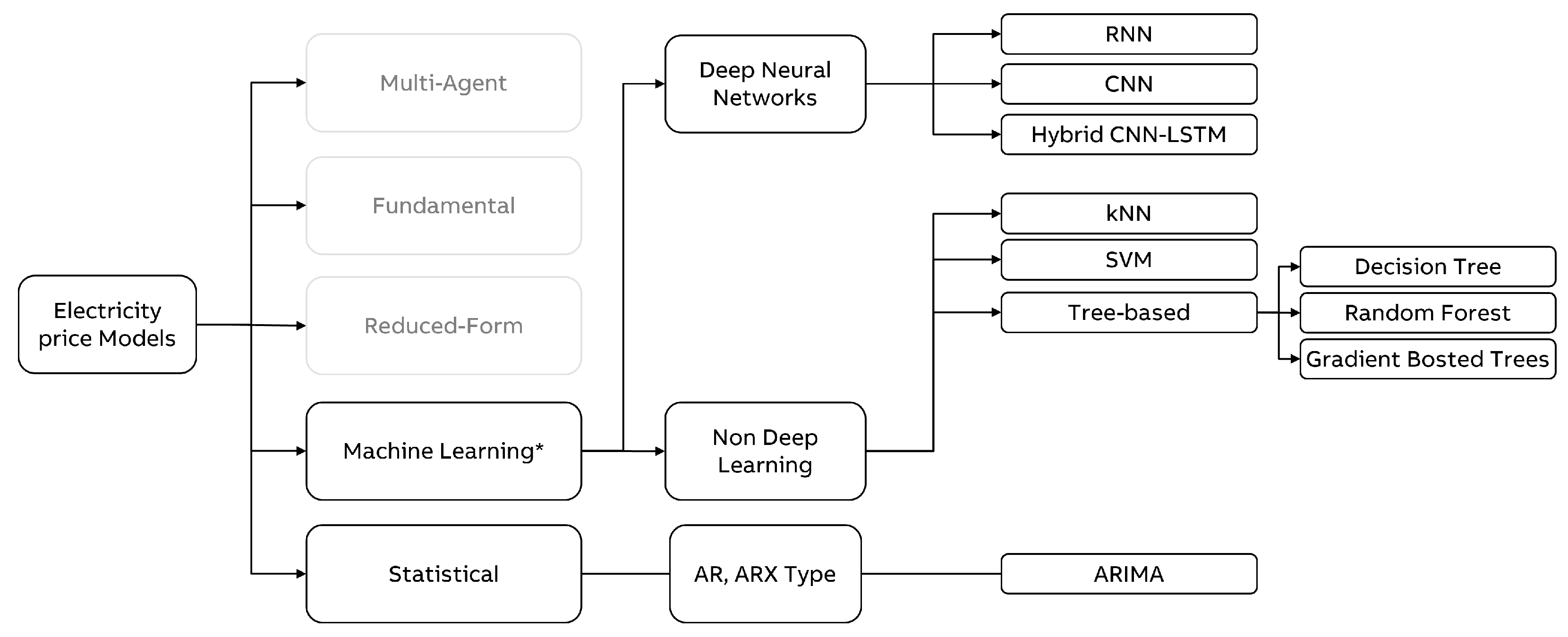
1.2. Techniques for Energy Market Prediction

Predictions about the energy market, especially energy prices, are highly relevant economically. Unsurprisingly, a large number of different approaches exist. Weron et al. [10] show an attempt to classify modeling approaches according to the state of knowledge at that time, which we extended to capture the methods considered in this comparative study:

• Multi-Agent Approaches
  Model the behavior of different actors on the market by algebraic or differential equations and solve the equation systems to find the market equilibrium, such as the Nash Cournet Framework or Supply function equilibrium. Borenstein, Bushnell, and Knittel [24] or Cabero et al. [25] are worth mentioning for a sample application of the former and, e.g., Baldick et al. [26] of the latter one, respectively. An alternative approach is to simulate the market with the help of agent-based simulation models. This modeling approach is very flexible but requires many assumptions. Here, e.g., Guerci, Rastegar and Cincotti [27] can be referred to for further details.
• Fundamental or structural models
  These models explicitly incorporate fundamental physical and economic relationships in energy production and trading and predict prices with the help of the resulting overall model. These models require detailed information about plant and transmission capacities and demand patterns. They also require assumptions about the physical and economic relationships in the market. See, e.g., Kanamura and Ohashi [28], Coulon and Howison [29], or Aïd, Canou, and Langrene [30] as illustrative examples.
• Reduced-form models
  This class of models is inspired by financial models of price dynamics, where the intention is usually not to provide a precise hourly forecast. Instead, they aim to capture the characteristics of daily electricity prices, mainly as an input to risk analysis. Jump diffusion models (see Carea and Figueroa [31]) and Markov regime-switching models (see Hamilton [32]) can be considered as typical examples.
• Statistical models
  Statistical forecast of the current price by a mathematical combination of previous prices and/or previous or current values of exogenous factors. Among others, exponential smoothing (see Cruz, Muñoz, Zamora, and Espinola [33]), regression models (e.g., Kim, Yu and Song [34]) or AR-type time series models (see Cuaresma, Hlouskova, Kossmeier, and Obersteiner [35]) are typical approaches in that regard.
• Computational intelligence models
  They are supposed to be nature-inspired computational techniques. Weron et al. [10] names here neural networks and support vector machines. See Chen, Dong, Meng, Xu, Wong, and Nagan [36], Garcia-Ascanio and Mate [37], Gareta et al. [38], or Mandal et al. [39] for the usage of neural networks, and Sansom, Downs, and Saha [40], among others, for SVM usage related to Energy Price Forecasting. To reflect the change in the perception of these methods in recent years, we decided to refer to this model type as a machine learning model.

The focus of this work is price forecasts for the spot market. Therefore, reduced-form methods were not further investigated, focusing on modeling market dynamics and providing input to risk analysis. Multi-agent approaches and fundamental models require much information about the market and assumptions about the physical and economic relationships. Making valid assumptions based on limited information and an increasing number of market actors is a challenging task. Hence, this work focuses on a statistical model and the taxonomy class that Weron et al. [10] referred to as a computational intelligence model. We decided, however, to call them machine learning-based approaches. Figure 2 shows the different models we evaluate in our work in the context of the taxonomy suggested by [10]. The following sections discuss the models in more detail.

2. Models

The following subsections briefly introduce each model considered in our experimental study. The ordering follows the modified taxonomy from [10] as shown in Figure 2.

2.1. Statistical

A classical approach to energy price forecasting involves using statistical models, such as AR, ARMA, ARIMA, and related methods, based on mathematical operations on historical prices.

• ARIMA Autoregressive integrated moving average (ARIMA) is a statistical time-series forecasting method combining an auto-regressive part [41], differentiating, and a moving average process. In this model, the future value is assumed to be a linear function of past observations and random errors. ARIMA models are widely used due to advantages such as simple structure and low computational complexity, as well as stable forecasting performance and capability to incorporate the seasonality factor prevailing in electricity price developments. In the presence of spikes, however, statistical methods perform relatively poorly. In addition, they struggle to capture the nonlinear fluctuation of market prices [10,42,43,44].

2.2. Machine Learning

Machine learning techniques have been widely adopted for energy price forecasting. They attempt to discover patterns in historical data and create predictions based on characteristic patterns.

2.2.1. Non Deep Learning

Canonical machine learning models include, for example, SVMs, kNN, and tree-based techniques. Existing literature reveals mixed results regarding their capability of appropriately forecasting electricity prices [15,45,46]. However, since some authors demonstrate their efficiency and advocate the utilization of SVMs [40,47,48,49] as well as of tree-based-techniques [50,51], we opted to include them in the present model comparison. Only a few studies assessed kNN on forecasting time series data, although it could be shown that they can outperform simple statistical methods under certain constraints [52]. The Naive forecaster is described in Section 2.2.3 and is used as a baseline model for our work.

• kNN
  K-nearest-neighbors (kNN) is a training-free method that makes predictions by averaging observations with features closest to the input sample. The method of k-nearest neighbors is conceptually simple and explainable. They do not make assumptions about the data and work well with non-linear relationships, often producing accurate predictions. However, the method becomes unfeasible with large data sets or numerous features. kNNs are unable to extrapolate beyond the range of the training data and are sensitive to noisy and irrelevant features. Another limitation is sensitivity to the number of neighbors k to be compared with, and the chosen neighbor distance metric [53].
• SVM
  Support vector machines (SVMs) work by detecting a hyperplane in a higher dimensional space with minimal distance to the fitted observations [54]. SVMs can solve linear and non-linear problems due to the ‘kernel trick’, implicitly mapping their inputs into high-dimensional feature spaces and then using simple linear functions to create linear decision boundaries in the new space. SVMs have become a common energy price forecasting method due to a variety of strengths, such as good approximating accuracy and generalization ability to unseen data, superior performance for small-scale training data, tolerance to redundant and highly interdependent features, as well as the capacity mentioned above to solve both linear and non-linear problems. The main challenges associated with SVM models are the computational costs of training, selection of a kernel function and parameters, sensitivity to noise and missing values, overfitting, and lack of explainability [10,42,44,46].
• Decision Trees, Random Forests and Gradient Boosted Trees
  Other popular methods are decision trees, random forests (making predictions by averaging a set of decorrelated trees built in parallel [55]), and gradient-boosted trees (which build an ensemble of trees iteratively by fitting a new tree on the residuals of the previous tree [56]). Decision trees are fast and interpretable: by retrieving the decision path for a given sample, one can see which feature values are used as criteria for the prediction. They can combine numerical and categorical features and capture non-linear relationships between features and the dependent variables. Trees are invariant under monotone transformations of individual features, robust concerning overfitting, and tolerant to outliers and missing values. Since feature selection implicitly occurs during training, decision trees are insensitive to irrelevant or interdependent features [53,55]. A relatively low accuracy limits them. The low accuracy, however, is alleviated by ensembling methods, for instance, random forests or gradient-boosted trees, which help increase prediction accuracy while maintaining all the benefits of decision trees, except for the loss of interpretability [46].

2.2.2. Deep Learning

Deep Learning methods are compelling when uncovering complex patterns, especially in extensive and high-dimensional data. Energy price prediction falls into that category since it is characterized by solid temporal patterns and high fluctuations—even within short periods. Previous research shows that several types of neural networks have proven well suited to handle these sequential relationships well [45,57,58,59,60,61].

• RNN
  While simple neural networks, such as fully connected feed-forward neural networks (FNN), are limited regarding sequential data, more sophisticated approaches have evolved [62]. So-called recurrent neural networks (RNN) are developed precisely for capturing sequential patterns and, thus, time series data. Instead of processing each timestamp independently and the entire sequence simultaneously, these models pursue a more dynamic approach: They process information incrementally and sequentially while creating an internal memory state on the fly—based on the previously provided content [63]. A particular performant kind of RNN is Long Short-Term Memory (LSTM), which can learn to recognize and store input and decide which information to preserve and which to forget. The key idea is to prevent older signals from gradually vanishing as the sequence elements get passed through the network [64]. This behavior is achieved by a memory block consisting of one or more memory cells and additional gates. The gates are an input gate, a forget gate, and an output gate. They control the information flows process [65].
• CNN
  Another architecture to solve machine learning applications are convolutional neural networks (CNN) [66]. Originally designed to handle image data efficiently, this type of network shows its strengths when automatically extracting the most relevant features of grid-like data, such as images, text, or even time series. Whereas FNNs aim to learn global pattern given the entire input at once, CNNs focuses on spatially close or local patterns by applying kernels (a.k.a. filters or convolutions) over a subsection of input data. For image data, one or more kernels get sliced across an image, stopping at each subsection (a patch or chunk of the image, e.g., a few pixels) and applying the same transformation (called “convolution”) on it. The output of each transformation is a feature map that encodes specific aspects representative of each subsection [62]. Analogous to capturing relevant features across two dimensions in an image (along the height and width axes), this operation is also applied to time series data in that the sequence is treated like a one-dimensional image. The convolution operates over a 1D sequence in this regard, returning a 1D feature map for each subsection (e.g., a few timestamps) [67]. Because a CNN in its traditional structure does not consider the temporal dependence between past and future data, its isolated, plain application on time series data is not considered part of this comparison.
• Hybrid CNN-LSTM
  However, to potentially improve the learning process of LSTMs even further, some authors suggested combining the benefits of LSTMs and CNNs—notably, feature extraction and forecasting [57]. Accordingly, the idea contains two steps: The first step comprises a CNN part to extract the time-domain characteristics prevalent in different periods (e.g., days or weeks) to reduce frequency variation. The CNN is followed by an LSTM part, which—provided with the salient time series features—ought to efficiently capture the temporal dependencies within the previously constructed feature maps. Given an input of multivariate time series, the CNN applies a 1D convolution on each time series by sliding a 1D kernel (Instead of applying 1D filters on multiple time series simultaneously, an informative reader might also come up with the idea to stack the multivariate time series horizontally and use a single 2D-CNN with a two-dimensional kernel, that processes the input horizontally and vertically. The results turned out to be the same) vertically to the right (as time passes) to create corresponding time-domain feature maps. The output (feature maps with a specified width and a height of 1) gets transmitted to the LSTM layer(s). Two final dense layers deliver the prediction for a desired forecasting horizon.

2.2.3. Baseline

The Naive model makes forecasts using past data as predictions, copying the latest available value in the sequence. To account for seasonal patterns, e.g., the last value in the sequence can be represented by the value from the previous hour, the previous day, or in this case, the previous week. This model serves as the baseline model and gets compared to those mentioned above.

3. Materials and Methods

This chapter describes the structure of the data for the forecasts and explains the evaluation scenarios. A description of the model fitting approach and the statistical evaluation of the model results is provided.

3.1. Data Set

In the following subsections, the data set, as well as its processing and splitting, is explained. For simplicity and better readability, we call the non-stationary data set ‘raw’ data as the actual target variable remains untouched in the steps described below, except for scaling.

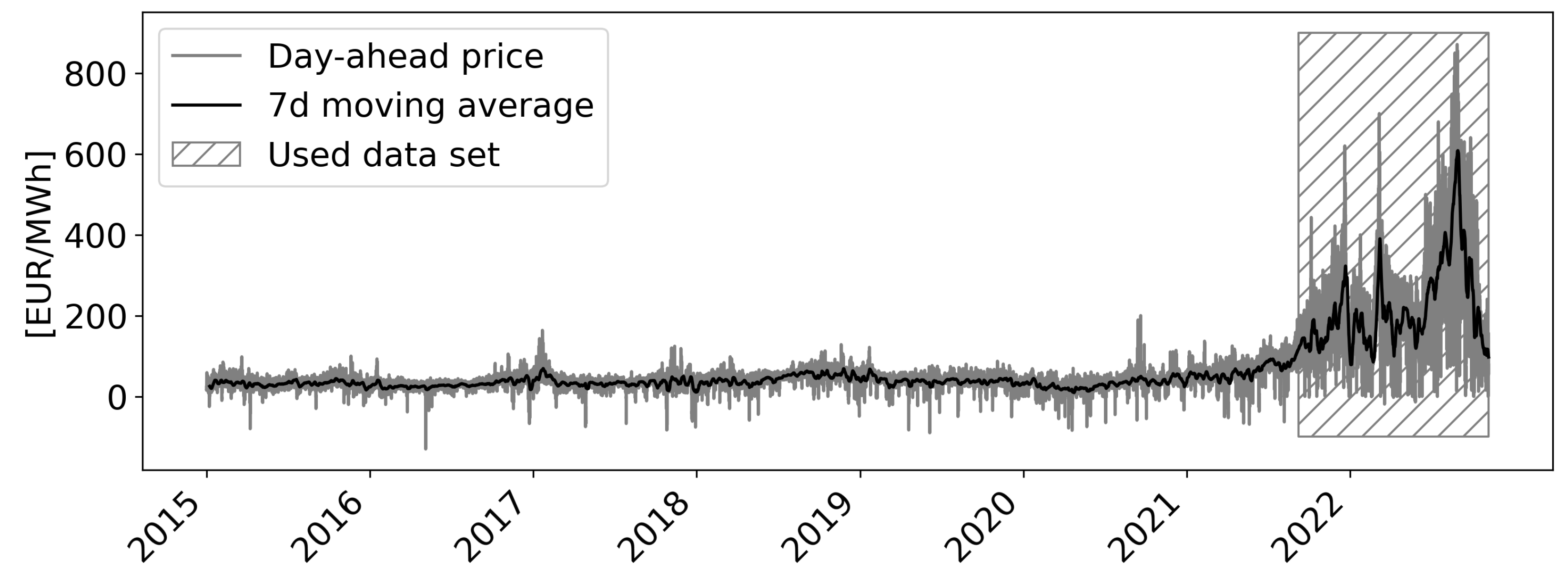
• Raw data
  The data set in this study consists of various publicly available weather data of the German Weather Service DWD [68] as well as market data from ENTSO-E [8]. The weather data set comprises measurements of several geographically distributed German weather stations, such as solar radiation, air pressure, wind speed, air temperature, and dew point temperature. The market data includes the traded spot market prices on the EEX in Leipzig and prices for energy sources such as Anthracite (hard coal) and natural gas. Overall, the complete data set contains more than 100 input variables. Although decades of historical data are available, this study focuses on data from recent years only, as a substantial shift in the data can be observed over the years (see Figure 1). Precisely, the data set starts on 9 September 2021 and covers the period until 1 November 2022—collected in hourly frequency.
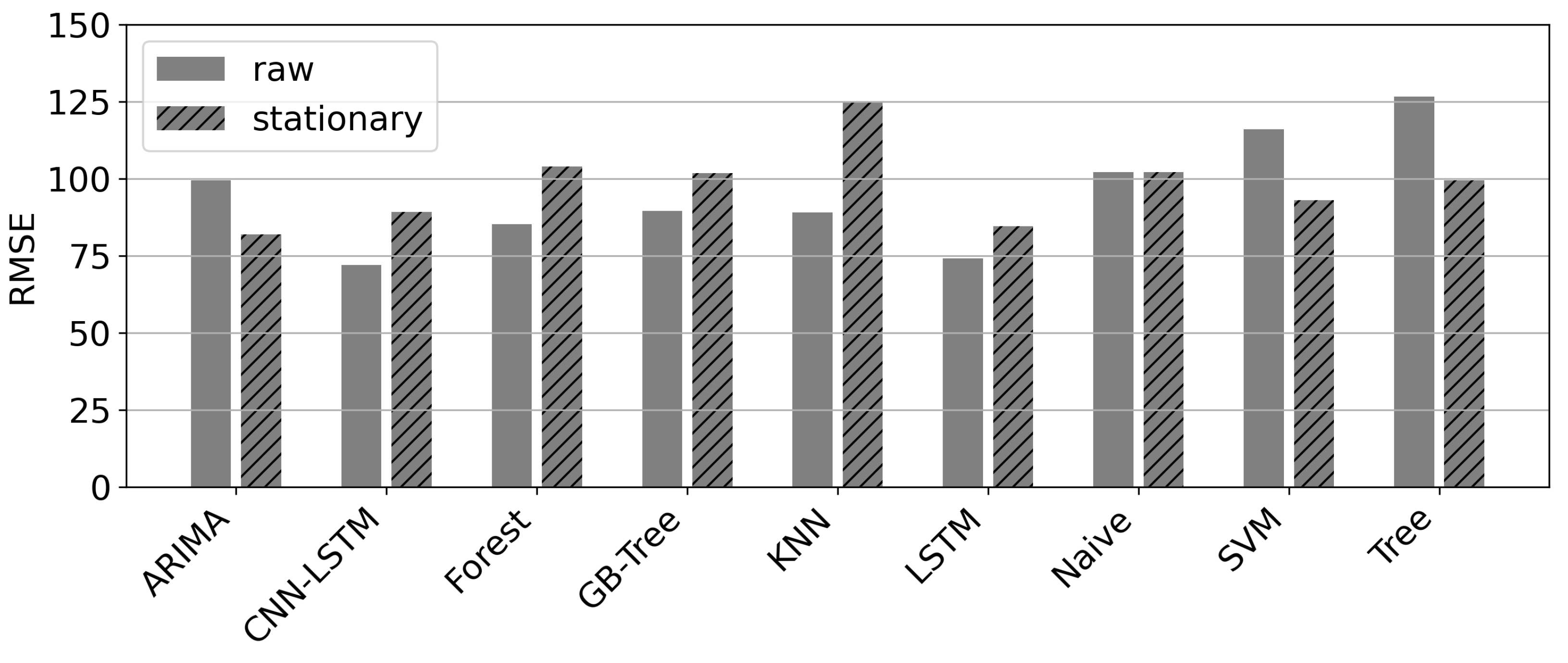
• Feature Engineering and Preprocessing
  The collected raw data undergoes a comprehensive pre-processing pipeline, including the following steps:
  At first, date-related features, such as an hour, day of the week, and day of the year, are transferred to a geometric representation with sine and cosine to prevent jumping transitions between two days, months, or years. Also, because the natural gas price is the only variable published daily instead of hourly, this variable must be forward-filled without any interpolation until the next available value to get an hourly resolution. Missing values in the weather data set are imputed by a k-Nearest-Neighbor (kNN) algorithm.
  A principal component analysis (PCA) on the weather data is performed To speed up the training process and improve the quality of the analysis, as they have shown to be highly correlated. The number of components depends on the explained variance; over 90% of the underlying information persists. Consequently, the weather data is reduced from 90 variables to 10.
  Since some algorithms cannot deal with time series with the trend or seasonal effects, a standard transformation of the target value in time series problems is to make them stationary. The data eventually approaches a stationary state by removing the daily and weekly periodicity and the removal of the inclining trend, verified by the Augmented Dickey-Fuller (ADFuller) and Kwiatkowski–Phillips–Schmidt–Shin (KPSS) test. Another step in the pre-processing pipeline is scaling input variables, notably by subtracting the mean and dividing by the standard deviation afterward; having all input variables in the same scale results in an improved model learning process. The same approach is applied to the target value as the final step.
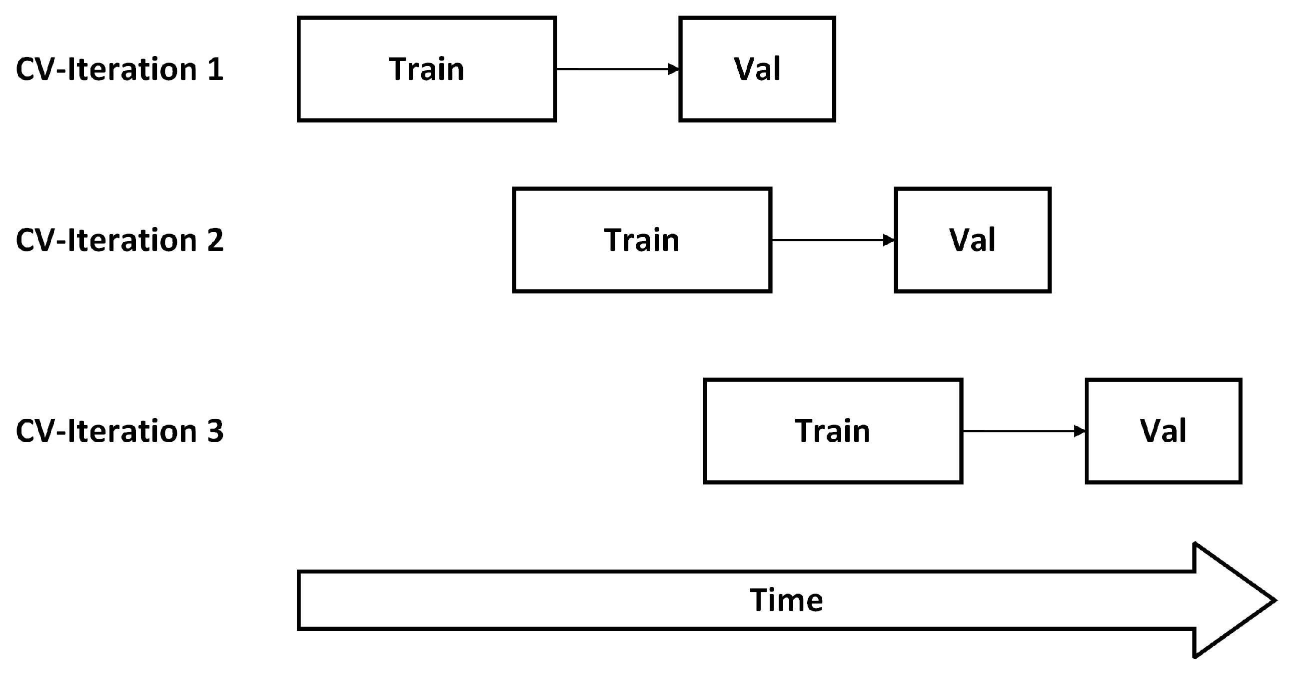
• Data split
  Finally, the processed data set is split into training, validation, and test set. The training set consists of 8760 samples of window size 168 (equal to 168 h), resulting in one year. A subsequent time series with identical length is held out for validation and testing. Further details will be part of Section 3.4.

3.2. Scenario Selection

In order to assess the robustness of different algorithms and their general ability to forecast different price scenarios in the following analysis section, three representative periods with different characteristics are selected. The three scenarios are determined by the day-ahead electricity prices’ mean and the standard deviation. The researchers of this study visually assess the prices. The goal is to have scenarios with high, moderate, and low mean electricity prices and a high, moderate, and low standard deviation. The approximated mean prices are 395, 250, and 110€/MWh, and the corresponding standard deviations are 80, 150, and 30€/MWh. Figure 3 gives an overview of the three selected scenarios:

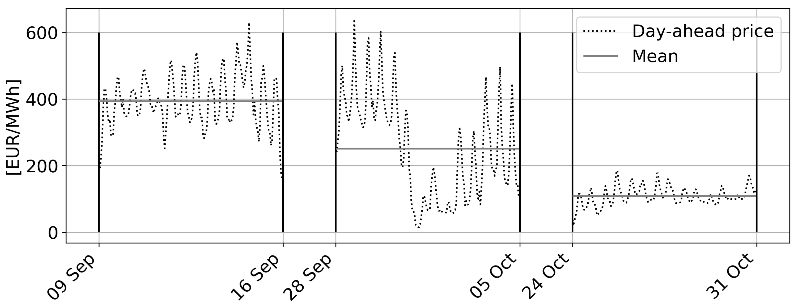
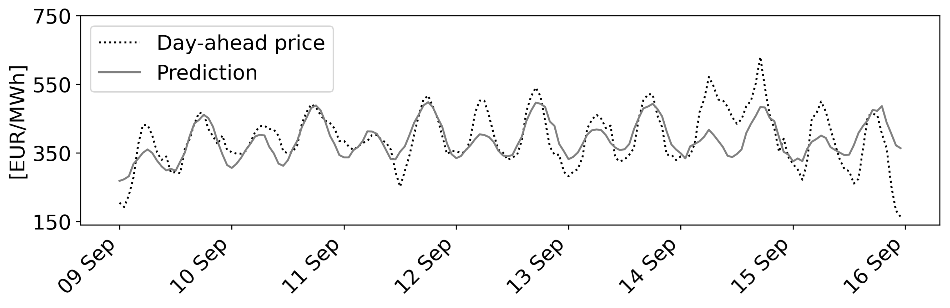
• Scenario 1 comprises the period from Friday, 9 September–Friday, 16 September 2022. This shows a day-dependent, cyclical behavior with normal price volatility.
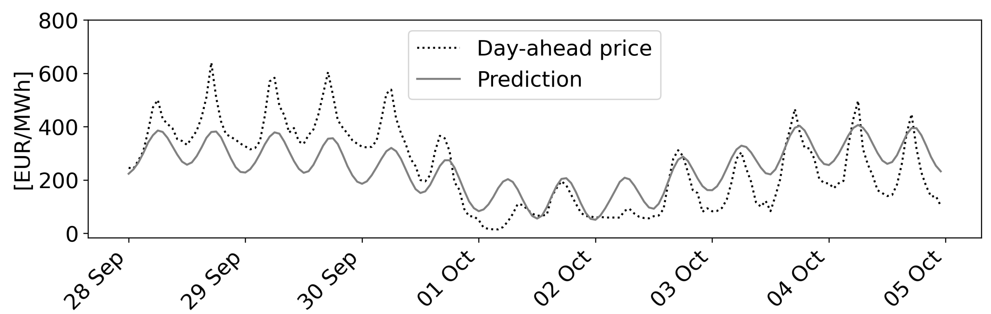
• Scenario 2 ranges from Wednesday, 28 September–Wednesday, 5 October 2022. It is characterized by high volatility and an acyclical price fall towards 0€/MWh.
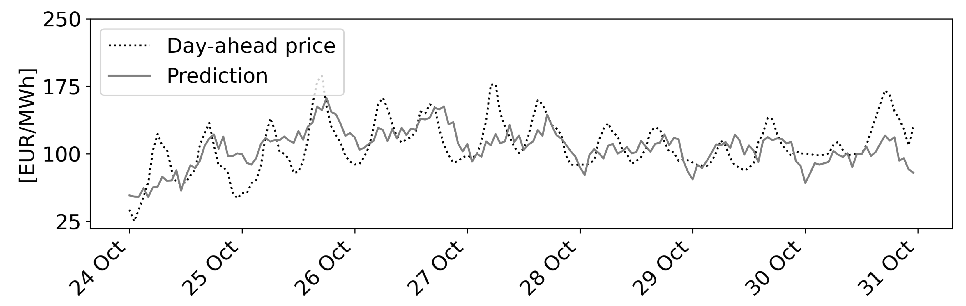
• Scenario 3 covers the period from Monday, 24 October–Monday, 31 October 2022 and shows low volatility and periodic prices with an offset of around −250€/MWh.

3.3. Model Fitting

Based on the three introduced scenarios, each model type is trained in a time-based k-fold cross-validation fashion over multiple hyperparameter configurations. For that, a sliding window approach is chosen as illustrated in Figure 4 below. It keeps the size of the training set constant while rolling the first point of the set forward. This approach is reasonable as it ensures a meaningful time series-specific validation and speeds the training process compared to an expanding window splitter. However, the expanding window splitter approach is computationally more expensive as it accumulates newly available data after each split. Another helpful feature is defining specific ’cut-off’ points (training set endpoints). This option allows the definition of the training windows following the scenarios. The final cross-validation setup encompasses three different splits moving over time using the sliding window splitter, where each of the splits contains a training set (cut-off date minus defined training set length of 8760 h in the past) and a validation set (cut-off date plus a defined forecasting horizon of 168 h into the future). In each iteration, a newly created model with identical initialization is trained.

All experiments are conducted by executing a pipeline built using the Python package sktime [70]. Data processing, such as scaling, transforming the original non-stationary data into static data, or reducing dimensionality, can be added as individual steps in the pipeline. This way, an identical setup can be ensured regardless of the training model. A fixed random seed is set to ensure that any of the observed differences between different experiments happen because of the model.

Hyperparameter tuning is implemented to determine a combination of parameters for each model in a grid search manner. This approach uses all combinations in a previously defined discrete search space. The researcher has to propose a list of values for each hyperparameter. As the number of hyperparameters differs among the model types, the total number of trained models may also differ. Furthermore, the deep learning models neither have default hyperparameters nor a default architecture. Instead, they must be built manually according to the researcher’s ideas. Moreover, the default hyperparameters of the non-deep learning models may skyrocket the computational effort as they are not adapted to the prediction task. Based on the performance of the validation set within each split (k = 3), the results of each combination are compared and ranked.

The entire routine, from data preprocessing to model evaluation, was performed on a single compute instance, ensuring reproducible results. This machine has a built-in Intel i9-11950H CPU, 32 GB RAM, an NVIDIA RTX A300 GPU, and Microsoft Windows version 10.0.19045.2364 installed on a Micron MTFDKBA1T0TFH NVME drive. No other applications ran in the background during training as they would slow down model fitting. The deep learning models are created with Keras version 2.10.0, as calculations can be performed on GPU to speed things up. The remaining models are created with either Scikit-Learn version 1.1.2 or SKTime version 0.13.4 running on the CPU. Besides that, the following software is installed: Python 3.9.12, CUDA 11.7, NVIDIA Driver 517.66, Pandas 1.5.0, and Numpy 1.22.4. The computational effort does not require a high-performance compute instance, and the experiment can be conducted within a few days. It is worth mentioning that not all models fully utilize the CPU, and hence, some cores are idle. Therefore, the model trainings can be run in parallel by starting another python instance.

3.4. Evaluation Criteria for the Algorithms

For the comparison among our conducted experiments, a variety of different error metrics are provided by the literature, such as Mean Absolute Error ($MAE$) see Equation (1), Mean Square Error ($MSE$), or Root Mean Square Error ($RMSE$) see Equation (2), a derivation of the $MSE$.

$$MAE=\frac{1}{n}\sum _{i=1}^n(P_i-O_i)$$

(1)

$$RMSE=\sqrt{\frac{1}{n}\sum _{i=1}^n{(P_i-O_i)}^2}$$

(2)

• $P_i$ is the predicted value for the ith observation in the dataset
• $O_i$ is the observed value for the ith observation in the dataset
• n is the sample size.

In this study, we use $RMSE$, a commonly used metric for evaluating the regression performance of forecasting models, to compare the quality of the predictions [71]. The $RMSE$ is a non-negative metric based on prediction errors, which penalizes undesirable significant errors but remains easily interpretable by being in the same unit as the target variable (EUR/MWh). Accordingly, each model is evaluated in all predefined configurations at different points in time. This is done in increments of 24 h before the end of the forecast horizon of 168 h.

4. Results

This section is divided into four subsections analyzing the general performance of the compared models from different perspectives. In the first subsection, the model robustness is investigated. The error metric allows us to conclude how stable the model types are. This is of interest if the model has to be as reliable as possible at the cost of minor performance losses. The second subsection is about the two data sets used in the experiments. Although this study focuses on model goodness, the chosen data set plays an important role, too. Interested readers get a recommendation regarding what machine learning model to select and if transformations should be applied to the data. The third subsection depicts the error history of the best candidates of each model type. As the $RMSE$ fluctuates from one-time step to another, it is of value to see how accurate the predictions are up to which point in time. In the last subsection, the best candidate of each model type, determined by averaging over all candidates, is evaluated. The predictions and the accurate day-ahead prices are plotted for all three scenarios. In contrast to the previous subsections, this last one focuses on qualitative analysis and gives insights into how forecasts are perceived.

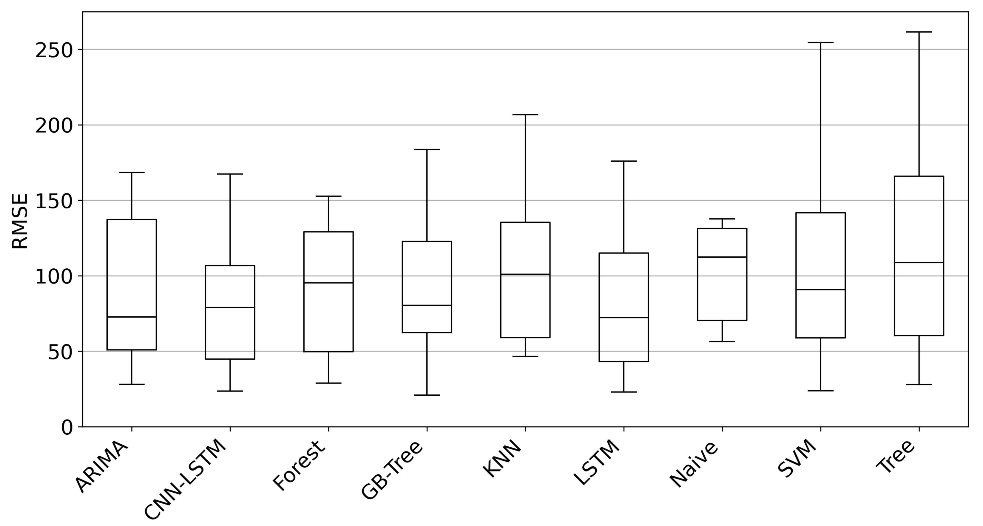
4.1. Model Robustness

Table 1. Error metrics on average and of the best hyperparameter configurations.

	Average		Best
Model	RMSE	MAE	RMSE	MAE
LSTM	79.33	64.52	59.92	48.45
CNN-LSTM	80.52	65.16	59.15	46.18
ARIMA	90.67	75.80	81.93	68.21
Random Forests	94.54	81.24	73.20	59.73
Gradient Boosted Trees	95.65	80.70	72.83	61.10
Naive	102.07	79.90	102.07	79.90
SVM	104.45	90.42	64.06	52.41
KNN	106.97	88.82	83.50	68.98
Decision Trees	113.01	98.60	86.80	70.47

depicts the aggregated results over all three test scenarios and hyperparameter configurations. As this study aims to assess each model type’s general performance, we choose the mean $RMSE$ as a relevant metric for the model comparison. Its overall error rank determines the best model. All hyperparameter setups are sorted in ascending order and get a rank assigned. This procedure is repeated for the error metrics $MAE$ and $RMSE$. As the results ranking of the $RMSE$ and $MSE$ are identical, the latter will be disregarded in further analysis.

Thus, the overall error rank is the sum of the individual error ranks of $MAE$ and $RMSE$. After calculating the ranks for the two metrics and ranking all the models according to this sum in ascending order, LSTMs are the best-performing models across the defined scenarios. It achieves an average $RMSE$ of 79.33, with the best configuration $RMSE$ of 59.92. The second best model type is a hybrid of CNN and LSTM. The best CNN-LSTM configuration achieves slightly better overall results across the scenarios than the LSTM. However, the improvement appears insignificant. The best LSTM model will be used for further analysis as its complexity is lower and has no performance loss over the CNN-LSTM model. The decision tree model has an $RMSE$ of over 110 and is approximately 40% worse on average. The Naive forecaster, the baseline model of this study, is a good model on average. SVM, kNN, and decision trees are worse on average. However, all well-tuned machine learning models achieve better results than the Naive model.

Figure 5 shows the error distributions across all hyperparameter setups and test scenarios. The decision tree stands out negatively as its mean, median, and total error deviation is higher than other models. SVMs are slightly better but also come with large deviations. The random forest has a relatively low deviation and is, therefore, a more robust model that is less sensitive to the choice of hyperparameters or the respective test scenario.

4.2. Data Set

Figure 6 Model quality concerning the utilized data set. The ARIMA model delivered better results on the stationary data set. All but two machine learning models can handle the raw data better than the transformed data. Using this insight, one can decrease the $RMSE$ by around 10. The Naive forecaster is transformation invariant as past data are directly used for predictions.

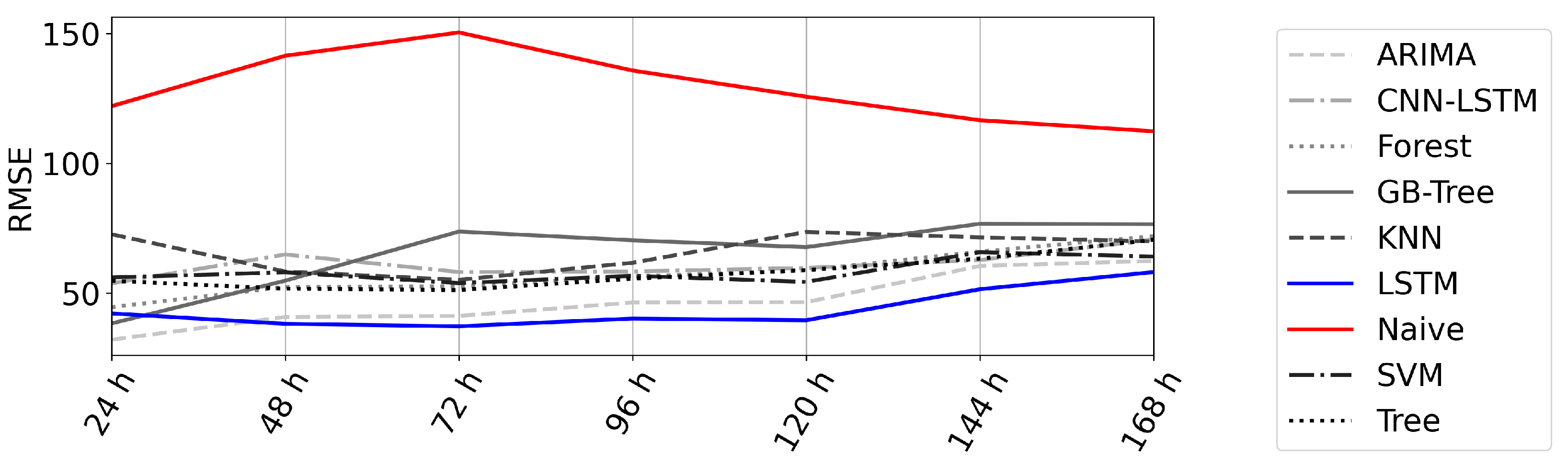
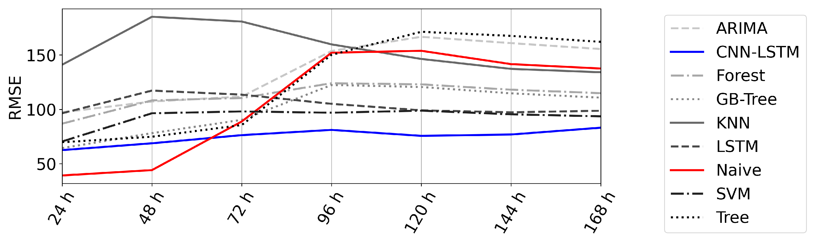
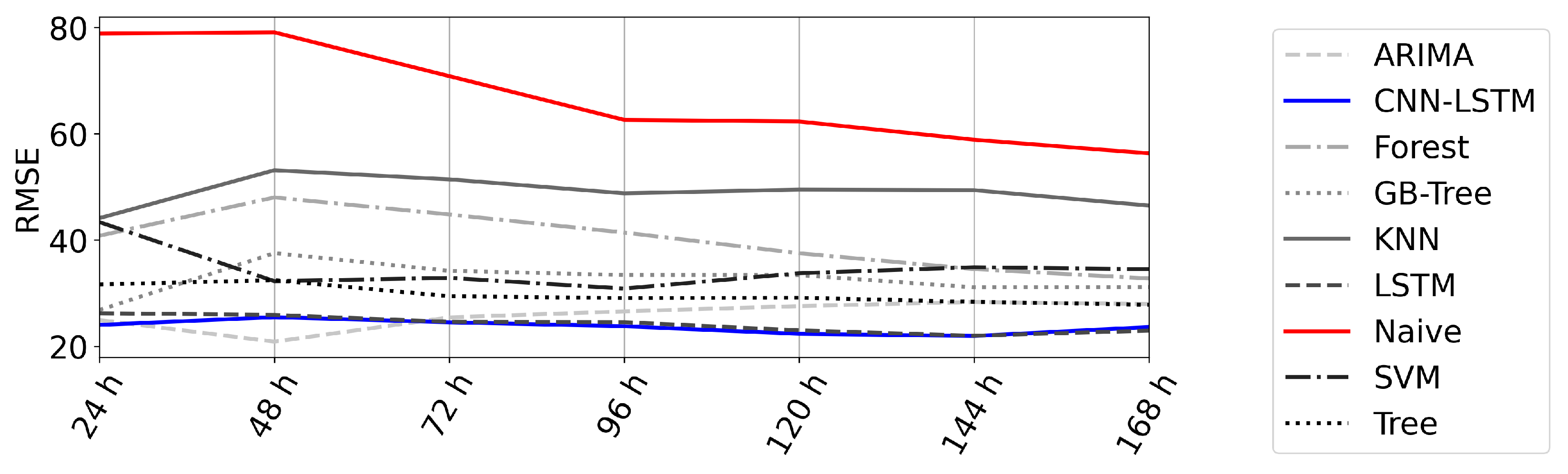
4.3. Error over Time

The following figures illustrate each model’s error behavior within the three defined test scenarios over time. The best hyperparameter configurations are chosen, but each test scenario results in a new model trained on a different data set.

As expected, a slight but general upward trend for all the models over time can be observed, as shown in Figure 7. The naive model performs worst, and its error is twice as large as the error of the LSTM model on test scenario 1. The LSTM stands out and has the lowest error from day two on. The remaining models perform similarly over time with minor deviations.

In Figure 8, one can observe that the overall error is generally higher than for test scenario 1. Furthermore, the deviation is more significant as well. The Naive model’s accuracy dropped considerably towards the horizon of 96 h. The CNN-LSTM architecture performed best.

The last diagram of this subsection, Figure 9, of the temporal error analysis follows a similar pattern to test scenario 1. Contradictory to our assumption that the error grows over the forecast horizon, the error is stable and even gets smaller for some models eventually. This is due to a shift in the day-ahead price.

4.4. Predictions

The last subsection of the result section evaluates the best LSTM candidate from a qualitative point of view. The LSTM was chosen because it is the model with the lowest $RMSE$ on average. In order to get concrete forecasts for all three test scenarios, a single model has to be taken. It is worth mentioning that the training process was executed thrice with identical hyperparameters and model initialization. The only difference between the test scenarios is the data set used for training and testing. The best hyperparameter set is considered the best choice for all scenarios as they perform best on average.

Figure 10, Figure 11 and Figure 12 show the forecasts of the best LSTM model. The cyclical pattern is predicted fairly well and is aligned with the actual day-ahead prices. Neither overshooting nor undershooting happened over the forecast period. However, a price spike on September 14th is not detected, and a drop at the end of the forecast horizon is not predicted.

Test scenario 2 is more challenging to predict as the cyclical pattern is interrupted by a price drop. Nonetheless, the LSTM predicted the price fall early, characterized by a declining trend. The recovery of the price, starting about two days after the price drop, is correctly identified as well. Overshooting is not an issue, but undershooting can be observed in tAhe forecasts for the first three days.

The last scenario adds complexity as the cyclical pattern is not steadily continuing, there is a price offset, and the overall volatility is higher. This pattern is also seen in the predictions. They are substantially more volatile and less smooth than the other two test scenarios. Despite the high fluctuation, both overshooting and undershooting are observed.

5. Discussion

Table 1 shows that LSTM models, on average, predict the energy market prices with the highest accuracy in all three defined scenarios. This result is consistent with findings of several publications using training and validation data prior to 2020 [15,16,17,18,19]. LSTM models are suggested to be especially suitable for handling non-linear, complex dependencies over time. The energy market is a prime example due to its volatility and highly distinctive seasonal characteristics [10,11]. Unforeseeable exogenous events (e.g., pandemics, wars) complicate predictions even further and thus make it difficult to accurately predict price jumps multiple days ahead, as these market-changing events are not present as input features. While allegedly simpler algorithms seem not to be powerful enough to capture the highly dynamic, non-linear stochastic nature of energy prices, neural networks with their flexible mechanisms, for example, to learn what parts of history to ’remember’ and what to ’forget’ in a given sequence, tend to be more appropriate as they are specifically designed to solve such kind of problems [65]. A second criterion is model robustness because a more robust model can be expected to be less sensitive to changes in the data distribution over time. A robust model is given if the model goodness deviates only slightly when hyperparameters change. This does not include generalizability, where training and validation errors are tightly coupled. Model robustness explains how much the predictions change depending on which hyperparameter and validation data are selected. The results also show that LSTM models work well on raw time-series data, simplifying the modeling pipeline and reducing the degrees of freedom that need to be considered during model training. However, some authors recommend variance stabilizing transformations [72,73] or outlier detection to remove price spikes [14]. In order to see how our models deal with these spikes and how they perform, we deliberately chose not to use any of these correcting methods. In the given context of power plant control operations, sharp price spikes are part of the signal. They are particularly interesting for energy technologies that can reach high dynamics (e.g., power to heat, controllable loads). The results also show that among the other model types, ARIMA requires the data set to be stationary [41]. There needs to be a consensus about using static data for the remaining machine learning models, just weak indications of the raw data.

In the German and European energy markets, it has become common for market participants to base their decisions on forecasts in recent years. Due to the ratio of market participants and volumes traded, it is doubtful that a forecast will give any single market participant a decisive advantage. This applies to suppliers as well as buyers and network operators. This leads to a better balance between supply and demand and reduced dispatch costs.

The practical results of this study are currently being tested by dispatchers in the Power Plant Dispatching Department and have a weighted influence on decision-making in power plant operation. The forecasts are used in addition to forecasts from third parties, thus increasing the data basis for decisions. Future developments should focus on explainability to answer questions like “why fly ups/downs occur?” “how much is each predictor going to price?” or “are my predictors plausible?”.

One limitation of the presented experimental results is the model evaluation metric. Other possible metrics indicate robustness (e.g., MAPE, DAE, and normalized variants of commonly used metrics [14]). However, $RMSE$ is the most suitable metric, as it penalizes outliers quadratically. Furthermore, $RMSE$ is valuable for its ease of interpretation due to unit conservation, here EUR/MWh. Another limitation when comparing the models based on the provided results is that all prediction steps have equal weight—a prediction error in the next time step is as critical to the models as the prediction error one week ahead. This error can be observed in scenarios 1 and 3, where no strictly monotonous behavior exists. Depending on the specific use case, using shorter prediction horizons and combining models with different prediction horizons might be beneficial. Predictions might become vague if the chosen forecast horizon is too long. Power plants capable of quick adjustments may benefit from shorter forecast periods as the difficulty of the modeling task decreases. Hence, the predictions become more accurate. Lastly, a possible quality criterion is the smoothness of the predictions. Even though the training setup is identical, there is no guarantee of smooth predictions, being spikey or erratic. This phenomenon might be due to the training data, as it can only be observed in test scenario 3. Nonetheless, regularization methods exist to ensure generalizability which can smoothen the predictions such as dropout or noise injection. Based on our investigations, this concept can be applied to any neural network to improve them further. With the application of regularization methods, overfitting is likely to be prevented as the random process of dropout and noise injection makes any training iteration unique. The constrained model becomes more robust as the training is more challenging.

Comparing our investigated approaches for each scenario supports the global finding: A deep learning model predicts all scenarios most accurately. Since the scenarios are unique, each possesses a challenge that needs to be solved. A sharp decline within a seasonal pattern characterizes scenarios 1 and 3. Scenario 2 adds difficulty because it consists of a seasonal decrease and a heavy negative trend. The idea of the hybrid approach is to reduce the noise of the given input and to extract the most relevant features only. Here, filtering facilitates the process of keeping the focus on the relevant parts. The filtering finally enables closer predictions but also implies trade-offs. For example, it is possible that the smoothing effect becomes too strong and destroys crucial parts of the sequence. In that case, the LSTM will not be able to predict the original time series problem very accurately anymore [67].

Taking a step back and considering the problem more extensively, additional future research work can be identified. The overall goal is to build a robust energy-price prediction system that requires minimal human effort in operation. However, more comprehensive measures are needed to build an ML solution suitable for a power plant control software system incorporating cross-dependencies between data, models, code, and configurations [74]. Lastly, model explainability techniques [75], and uncertainty quantification [76] need to be incorporated to support the predicted results’ reasoning well as gain trust and transparency for the high-impact decisions such a system facilitates. Using a dropout layer in a neural network during inference and repeat making forecasts multiple times is an approach to investigate uncertainty. By randomly shutting off neurons of a dense layer, the model gets into a situation where information gets discarded. This procedure forces the model to use all input features and not rely on some features only [77]. Conformal predictions can provide additional insights that increase confidence in the prediction model. This approach returns prediction intervals instead of points. The point estimation made by the prediction model is guaranteed to be within the interval given a high probability [78]. Both methods aim to reason predictions, so power plant dispatchers gain confidence and trust in the application. They will be part of future work helping to understand how a fluctuating day-ahead electricity price causes forecast uncertainty.

6. Conclusions

In general, we were able to show in the study that there are algorithms that are particularly good at predicting electricity prices on the German spot market in times of economic and political tension. The algorithms can quickly anticipate changes in the price structure due to international events and predict with comparable quality. It should be emphasized that the daily and weekly patterns are modeled considering trends, jumps, and other disturbances. In principle, all models examined deliver beneficial results, although the deep learning models are the most suitable for predicting the patterns of the price signal. The following conclusions can be drawn from the research:

• Deep learning models are well suited for the prediction of time series in the interval of 168h in times of economic and political tension.
• The use of raw data has a positive influence on the error for best models/all deep learning models (RMSE decreases by approx. 10).
• Models based on CNN are best able to reproduce extreme values (fly up/down).
• Hyperparameter optimization can reduce the RSME by 20.
• The forecast error did not significantly rise with the forecast horizon.

References

- Lu, H.; Ma, X.; Ma, M.; Zhu, S. Energy price prediction using data-driven models: A decade review. Comput. Sci. Rev. 2021, 39, 100356. [Google Scholar] [CrossRef]
- Bento, P.; Mariano, S.; Calado, M.; Pombo, J. Impacts of the COVID-19 pandemic on electric energy load and pricing in the Iberian electricity market. Energy Rep. 2021, 7, 4833–4849. [Google Scholar] [CrossRef]
- Pradhan, A.K.; Rout, S.; Khan, I.A. Does market concentration affect wholesale electricity prices? An analysis of the Indian electricity sector in the COVID-19 pandemic context. Util. Policy 2021, 73, 101305. [Google Scholar] [CrossRef]
- Lazo, J.; Aguirre, G.; Watts, D. An impact study of COVID-19 on the electricity sector: A comprehensive literature review and Ibero-American survey. Renew. Sustain. Energy Rev. 2022, 158, 112135. [Google Scholar] [CrossRef] [PubMed]
- Şahin, U.; Ballı, S.; Chen, Y. Forecasting seasonal electricity generation in European countries under COVID-19-induced lockdown using fractional grey prediction models and machine learning methods. Appl. Energy 2021, 302, 117540. [Google Scholar] [CrossRef]
- Bigerna, S.; Bollino, C.A.; D’Errico, M.C.; Polinori, P. COVID-19 lockdown and market power in the Italian electricity market. Energy Policy 2022, 161, 112700. [Google Scholar] [CrossRef]
- Pizarro-Irizar, C. Is it all about supply? Demand-side effects on the Spanish electricity market following COVID-19 lockdown policies. Util. Policy 2023, 80, 101472. [Google Scholar] [CrossRef]
- European Network of Transmission System Operators for Electricity (ENTSO-E). Transparency Platform. 2022. Available online: https://transparency.entsoe.eu (accessed on 6 December 2022).
- Deutscher Wetterdienst. DWD Climate Data Center (CDC). 2022. Available online: https://www.dwd.de/DE/leistungen/opendata/opendata.html (accessed on 14 December 2022).
- Weron, R. Electricity Price Forecasting: A Review of the State-of-the-Art with a Look into the Future. Int. J. Forecast. 2014, 30, 1030–1081. [Google Scholar] [CrossRef]
- Lago, J.; Marcjasz, G.; De Schutter, B.; Weron, R. Forecasting day-ahead electricity prices: A review of state-of-the-art algorithms, best practices and an open-access benchmark. Appl. Energy 2021, 293, 116983. [Google Scholar] [CrossRef]
- Brusaferri, A.; Matteucci, M.; Portolani, P.; Vitali, A. Bayesian deep learning based method for probabilistic forecast of day-ahead electricity prices. Appl. Energy 2019, 250, 1158–1175. [Google Scholar] [CrossRef]
- Li, W.; Becker, D.M. Day-ahead electricity price prediction applying hybrid models of LSTM-based deep learning methods and feature selection algorithms under consideration of market coupling. Energy 2021, 237, 121543. [Google Scholar] [CrossRef]
- Tschora, L.; Pierre, E.; Plantevit, M.; Robardet, C. Electricity price forecasting on the day-ahead market using machine learning. Appl. Energy 2022, 313, 118752. [Google Scholar] [CrossRef]
- Lago, J.; De Ridder, F.; De Schutter, B. Forecasting spot electricity prices: Deep learning approaches and empirical comparison of traditional algorithms. Appl. Energy 2018, 221, 386–405. [Google Scholar] [CrossRef]
- Mujeeb, S.; Javaid, N.; Ilahi, M.; Wadud, Z.; Ishmanov, F.; Afzal, M.K. Deep Long Short-Term Memory: A New Price and Load Forecasting Scheme for Big Data in Smart Cities. Sustainability 2019, 11, 987. [Google Scholar] [CrossRef]
- Guo, X.; Zhao, Q.; Zheng, D.; Ning, Y.; Gao, Y. A short-term load forecasting model of multi-scale CNN-LSTM hybrid neural network considering the real-time electricity price. Energy Rep. 2020, 6, 1046–1053. [Google Scholar] [CrossRef]
- Memarzadeh, G.; Keynia, F. Short-term electricity load and price forecasting by a new optimal LSTM-NN based prediction algorithm. Electr. Power Syst. Res. 2021, 192, 106995. [Google Scholar] [CrossRef]
- Keles, D.; Scelle, J.; Paraschiv, F.; Fichtner, W. Extended forecast methods for day-ahead electricity spot prices applying artificial neural networks. Appl. Energy 2016, 162, 218–230. [Google Scholar] [CrossRef]
- Roeger, W.; Welfens, P.J. Gas price caps and electricity production effects in the context of the Russo-Ukrainian War: Modeling and new policy reforms. Int. Econ. Econ. Policy 2022, 19, 645–673. [Google Scholar] [CrossRef]
- Osička, J.; Černoch, F. European energy politics after Ukraine: The road ahead. Energy Res. Soc. Sci. 2022, 91, 102757. [Google Scholar] [CrossRef]
- Meng, A.; Wang, P.; Zhai, G.; Zeng, C.; Chen, S.; Yang, X.; Yin, H. Electricity price forecasting with high penetration of renewable energy using attention-based LSTM network trained by crisscross optimization. Energy 2022, 254, 124212. [Google Scholar] [CrossRef]
- Yang, H.; Schell, K.R. QCAE: A quadruple branch CNN autoencoder for real-time electricity price forecasting. Int. J. Electr. Power Energy Syst. 2022, 141, 108092. [Google Scholar] [CrossRef]
- Borenstein, S.; Bushnell, J.; Knittel, C.R. Market power in electricity markets: Beyond concentration measures. Energy J. 1999, 20. [Google Scholar] [CrossRef]
- Cabero, J.; Baillo, A.; Cerisola, S.; Ventosa, M.; Garcia-Alcalde, A.; Peran, F.; Relano, G. A medium-term integrated risk management model for a hydrothermal generation company. IEEE Trans. Power Syst. 2005, 20, 1379–1388. [Google Scholar] [CrossRef]
- Baldick, R.; Grant, R.; Kahn, E. Theory and application of linear supply function equilibrium in electricity markets. J. Regul. Econ. 2004, 25, 143–167. [Google Scholar] [CrossRef]
- Rastegar, M.A.; Guerci, E.; Cincotti, S. Forward Contract Effects in the Italian Whole-sale Electricity Market. In Handbook of Power Systems II; Rebennack, S., Pardalos, P.M., Pereira, M.V.F., Iliadis, N.A., Eds.; Springer: Berlin/Heidelberg, Germany, 2010; pp. 241–286. [Google Scholar]
- Kanamura, T.; Ōhashi, K. On transition probabilities of regime switching in electricity prices. Energy Econ. 2008, 30, 1158–1172. [Google Scholar] [CrossRef]
- Howison, S.; Coulon, M. Stochastic behaviour of the electricity bid stack: From fundamental drivers to power prices. J. Energy Mark. 2009, 2, 29–69. [Google Scholar]
- Aïd, R.; Campi, L.; Langrené, N. A Structural Risk-Neutral Model for Pricing and Hedging Power Derivatives. Math. Financ. Int. J. Math. Stat. Financ. Econ. 2013, 23, 387–438. [Google Scholar] [CrossRef]
- Cartea, A.; Figueroa, M.G. Pricing in electricity markets: A mean reverting jump diffusion model with seasonality. Appl. Math. Financ. 2005, 12, 313–335. [Google Scholar] [CrossRef]
- Hamilton, J.D. Regime switching models. In Macroeconometrics and Time Series Analysis; Durlauf, S.N., Blume, L.E., Eds.; Palgrave Macmillan: London, UK, 2010; pp. 202–209. [Google Scholar]
- Cruz, A.; Muñoz, A.; Zamora, J.L.; Espínola, R. The effect of wind generation and weekday on Spanish electricity spot price forecasting. Electr. Power Syst. Res. 2011, 81, 1924–1935. [Google Scholar] [CrossRef]
- Kim, C.i.; Yu, I.K.; Song, Y. Prediction of system marginal price of electricity using wavelet transform analysis. Energy Convers. Manag. 2002, 43, 1839–1851. [Google Scholar] [CrossRef]
- Cuaresma, J.C.; Hlouskova, J.; Kossmeier, S.; Obersteiner, M. Forecasting electricity spot-prices using linear univariate time-series models. Appl. Energy 2004, 77, 87–106. [Google Scholar] [CrossRef]
- Chen, X.; Dong, Z.Y.; Meng, K.; Xu, Y.; Wong, K.P.; Ngan, H. Electricity price forecasting with extreme learning machine and bootstrapping. IEEE Trans. Power Syst. 2012, 27, 2055–2062. [Google Scholar] [CrossRef]
- Garcia-Ascanio, C.; Maté, C. Electric power demand forecasting using interval time series: A comparison between VAR and iMLP. Energy Policy 2010, 38, 715–725. [Google Scholar] [CrossRef]
- Gareta, R.; Romeo, L.M.; Gil, A. Forecasting of electricity prices with neural networks. Energy Convers. Manag. 2006, 47, 1770–1778. [Google Scholar] [CrossRef]
- Mandal, P.; Senjyu, T.; Funabashi, T. Neural networks approach to forecast several hour ahead electricity prices and loads in deregulated market. Energy Convers. Manag. 2006, 47, 2128–2142. [Google Scholar] [CrossRef]
- Sansom, D.C.; Downs, T.; Saha, T.K. Evaluation of support vector machine based forecasting tool in electricity price forecasting for Australian national electricity market participants. J. Electr. Electron. Eng. Aust. 2003, 22, 227–233. [Google Scholar]
- Box, G.E.; Jenkins, G.M.; Reinsel, G. Time Series Analysis: Forecasting and Control; Holden-Day, Inc.: San Francisco, CA, USA, 1970. [Google Scholar]
- Jiang, L.; Hu, G. A Review on Short-Term Electricity Price Forecasting Techniques for Energy Markets. In Proceedings of the 2018 15th International Conference on Control, Automation, Robotics and Vision (ICARCV), Singapore, 18–21 November 2018; pp. 937–944. [Google Scholar] [CrossRef]
- Luo, X.; Zhu, X.; Gee Lim, E. A Hybrid Model for Short Term Real-Time Electricity Price Forecasting in Smart Grid. Big Data Anal. 2018, 3, 8. [Google Scholar] [CrossRef]
- Patel, H.; Shah, M. Energy Consumption and Price Forecasting Through Data-Driven Analysis Methods: A Review. SN Comput. Sci. 2021, 2, 315. [Google Scholar] [CrossRef]
- Zhang, R.; Li, G.; Ma, Z. A Deep Learning Based Hybrid Framework for Day-Ahead Electricity Price Forecasting. IEEE Access 2020, 8, 143423–143436. [Google Scholar] [CrossRef]
- Ghoddusi, H.; Creamer, G.G.; Rafizadeh, N. Machine Learning in Energy Economics and Finance: A Review. Energy Econ. 2019, 81, 709–727. [Google Scholar] [CrossRef]
- Stathakis, E.; Papadimitriou, T.; Gogas, P. Forecasting Electricity Price Spikes Using Support Vector Machines. SSRN Electron. J. 2017. [Google Scholar] [CrossRef]
- Papadimitriou, T.; Gogas, P.; Stathakis, E. Forecasting energy markets using support vector machines. Energy Econ. 2014, 44, 135–142. [Google Scholar] [CrossRef]
- Zhao, J.H.; Dong, Z.Y.; Xu, Z.; Wong, K.P. A statistical approach for interval forecasting of the electricity price. IEEE Trans. Power Syst. 2008, 23, 267–276. [Google Scholar] [CrossRef]
- Díaz, J.; Romero, Á.; Dorronsoro, J.R. Day-ahead price forecasting for the spanish electricity market. Int. J. Interact. Multimed. Artif. Intell. 2018, 5, 42–50. [Google Scholar]
- Mei, J.; He, D.; Harley, R.; Habetler, T.; Qu, G. A random forest method for real-time price forecasting in New York electricity market. In Proceedings of the 2014 IEEE PES General Meeting|Conference & Exposition, National Harbor, MD, USA, 27–31 July 2014; pp. 1–5. [Google Scholar]
- Al-Qahtani, F.H.; Crone, S.F. Multivariate k-nearest neighbour regression for time series data—A novel algorithm for forecasting UK electricity demand. In Proceedings of the 2013 International Joint Conference on Neural Networks (IJCNN), Dallas, TX, USA, 4–9 August 2013; pp. 1–8. [Google Scholar] [CrossRef]
- Hastie, T.; Tibshirani, R.; Friedman, J. The Elements of Statistical Learning; Springer Series in Statistics; Springer: New York, NY, USA, 2009. [Google Scholar]
- Awad, M.; Khanna, R. Support Vector Regression. In Efficient Learning Machines: Theories, Concepts, and Applications for Engineers and System Designers; Apress: Berkeley, CA, USA, 2015; pp. 67–80. [Google Scholar] [CrossRef]
- Breiman, L. Random forests. Mach. Learn. 2001, 45, 5–32. [Google Scholar] [CrossRef]
- Friedman, J.H. Greedy Function Approximation: A Gradient Boosting Machine. Ann. Stat. 2001, 29, 1189–1232. [Google Scholar] [CrossRef]
- Kuo, P.H.; Huang, C.J. An Electricity Price Forecasting Model by Hybrid Structured Deep Neural Networks. Sustainability 2018, 10, 1280. [Google Scholar] [CrossRef]
- Chang, Z.; Zhang, Y.; Chen, W. Electricity price prediction based on hybrid model of adam optimized LSTM neural network and wavelet transform. Energy 2019, 187, 115804. [Google Scholar] [CrossRef]
- Zhang, C.; Li, R.; Shi, H.; Li, F. Deep Learning for Day-ahead Electricity Price Forecasting. IET Smart Grid 2020, 3, 462–469. [Google Scholar] [CrossRef]
- Huang, C.J.; Shen, Y.; Chen, Y.H.; Chen, H.C. A novel hybrid deep neural network model for short-term electricity price forecasting. Int. J. Energy Res. 2021, 45, 2511–2532. [Google Scholar] [CrossRef]
- Heidarpanah, M.; Hooshyaripor, F.; Fazeli, M. Daily electricity price forecasting using artificial intelligence models in the Iranian electricity market. Energy 2023, 263, 126011. [Google Scholar] [CrossRef]
- LeCun, Y.; Bengio, Y.; Hinton, G. Deep learning. Nature 2015, 521, 436–444. [Google Scholar] [CrossRef] [PubMed]
- Goodfellow, I.; Bengio, Y.; Courville, A. Deep Learning; MIT Press: Cambridge, MA, USA, 2016; Available online: http://www.deeplearningbook.org (accessed on 21 January 2023).
- Hochreiter, S.; Schmidhuber, J. Long Short-Term Memory. Neural Comput. 1997, 9, 1735–1780. [Google Scholar] [CrossRef] [PubMed]
- Gers, F.A.; Schmidhuber, J.; Cummins, F. Learning to Forget: Continual Prediction with LSTM. Neural Comput. 2000, 12, 2451–2471. [Google Scholar] [CrossRef] [PubMed]
- LeCun, Y.; Bottou, L.; Bengio, Y.; Haffner, P. Gradient-based learning applied to document recognition. Proc. IEEE 1998, 86, 2278–2324. [Google Scholar] [CrossRef]
- Chollet, F. Deep Learning with Python; Manning Publications: Shelter Island, NY, USA, 2021. [Google Scholar]
- European Energy Exchange AG. Basics of the Power Market. 2023. Available online: https://www.eex.com/en/ (accessed on 21 January 2023).
- SKTime. Sliding Window Schema. Available online: https://www.sktime.org/en/stable/api_reference/auto_generated/sktime.forecasting.model_selection.SlidingWindowSplitter.html (accessed on 17 January 2023).
- Löning, M.; Bagnall, A.; Ganesh, S.; Kazakov, V.; Lines, J.; Király, F.J. sktime: A unified interface for machine learning with time series. arXiv 2019, arXiv:1909.07872. [Google Scholar]
- Chai, T.; Draxler, R. Root mean square error (RMSE) or mean absolute error (MAE)?—Arguments against avoiding RMSE in the literature. Geosci. Model Dev. 2014, 7, 1247–1250. [Google Scholar] [CrossRef]
- Uniejewski, B.; Weron, R.; Ziel, F. Variance Stabilizing Transformations for Electricity Spot Price Forecasting. IEEE Trans. Power Syst. 2018, 33, 2219–2229. [Google Scholar] [CrossRef]
- Ziel, F.; Weron, R. Day-ahead electricity price forecasting with high-dimensional structures: Univariate vs. multivariate modeling frameworks. Energy Econ. 2018, 70, 396–420. [Google Scholar] [CrossRef]
- Sculley, D.; Holt, G.; Golovin, D.; Davydov, E.; Phillips, T.; Ebner, D.; Chaudhary, V.; Young, M.; Crespo, J.F.; Dennison, D. Hidden Technical Debt in Machine Learning Systems. Adv. Neural Inf. Process. Syst. 2015, 28. Available online: https://papers.nips.cc/paper/2015/hash/86df7dcfd896fcaf2674f757a2463eba-Abstract.html (accessed on 1 January 2023).
- Arrieta, A.B.; Díaz-Rodríguez, N.; Del Ser, J.; Bennetot, A.; Tabik, S.; Barbado, A.; García, S.; Gil-López, S.; Molina, D.; Benjamins, R.; et al. Explainable Artificial Intelligence (XAI): Concepts, taxonomies, opportunities and challenges toward responsible AI. Inf. Fusion 2020, 58, 82–115. [Google Scholar] [CrossRef]
- Abdar, M.; Pourpanah, F.; Hussain, S.; Rezazadegan, D.; Liu, L.; Ghavamzadeh, M.; Fieguth, P.; Cao, X.; Khosravi, A.; Acharya, U.R.; et al. A review of uncertainty quantification in deep learning: Techniques, applications and challenges. Inf. Fusion 2021, 76, 243–297. [Google Scholar] [CrossRef]
- Gal, Y.; Ghahramani, Z. Dropout as a Bayesian Approximation: Representing Model Uncertainty in Deep Learning. In Proceedings of the 33rd International Conference on International Conference on Machine Learning, New York, NY, USA, 19–24 June 2016; Volume 48, pp. 1050–1059. [Google Scholar]
- Angelopoulos, A.N.; Bates, S. A Gentle Introduction to Conformal Prediction and Distribution-Free Uncertainty Quantification. arXiv 2021, arXiv:2107.07511. [Google Scholar]