Conditional Temporal Aggregation for Time Series Forecasting Using Feature-Based Meta-Learning

Abstract

We present a machine learning approach for applying (multiple) temporal aggregation in time series forecasting settings. The method utilizes a classification model that can be used to either select the most appropriate temporal aggregation level for producing forecasts or to derive weights to properly combine the forecasts generated at various levels. The classifier consists a meta-learner that correlates key time series features with forecasting accuracy, thus enabling a dynamic, data-driven selection or combination. Our experiments, conducted in two large data sets of slow- and fast-moving series, indicate that the proposed meta-learner can outperform standard forecasting approaches.

1. Introduction

Forecasting is essential for supporting decisions at strategic, tactical, and operational levels. Accurate forecasts can assist companies and organizations in reducing costs, avoid risks, and exploit opportunities, thus finding application in a variety of settings. Nevertheless, univariate forecasting is a challenging task that usually requires identifying patterns in time series data and selecting the most appropriate model for extrapolating them in time. As a result, numerous approaches have been proposed to perform model selection [1]. Still, this selection process involves significant uncertainty, especially when the patterns of the series are complex or the data are noisy [2]. To deal with model uncertainty, forecasters have been combining (ensembling) forecasts of multiple models, each making different assumptions about the distribution and correlation of the data [3]. The practice of combining has been proved particularly effective in various forecasting studies and competitions [4] and many ensemble strategies have been suggested to exploit its full potential.

From the combination methods found in the literature, those that build on data manipulation and transformation are probably the most promising. Instead of training different models on the examined series and combining their forecasts, these methods transform the series to create new ones, each highlighting particular characteristics (typically called time series features) of the original data. Then, the same or different models can be used to forecast the transformed series. More often than not, combining these forecasts (typically called base forecasts) results in better forecasting accuracy. Petropoulos and Spiliotis [5] discuss how the “wisdom of the data” can be used to extract useful information from series and review various approaches that exploit its benefits in univariate forecasting settings.

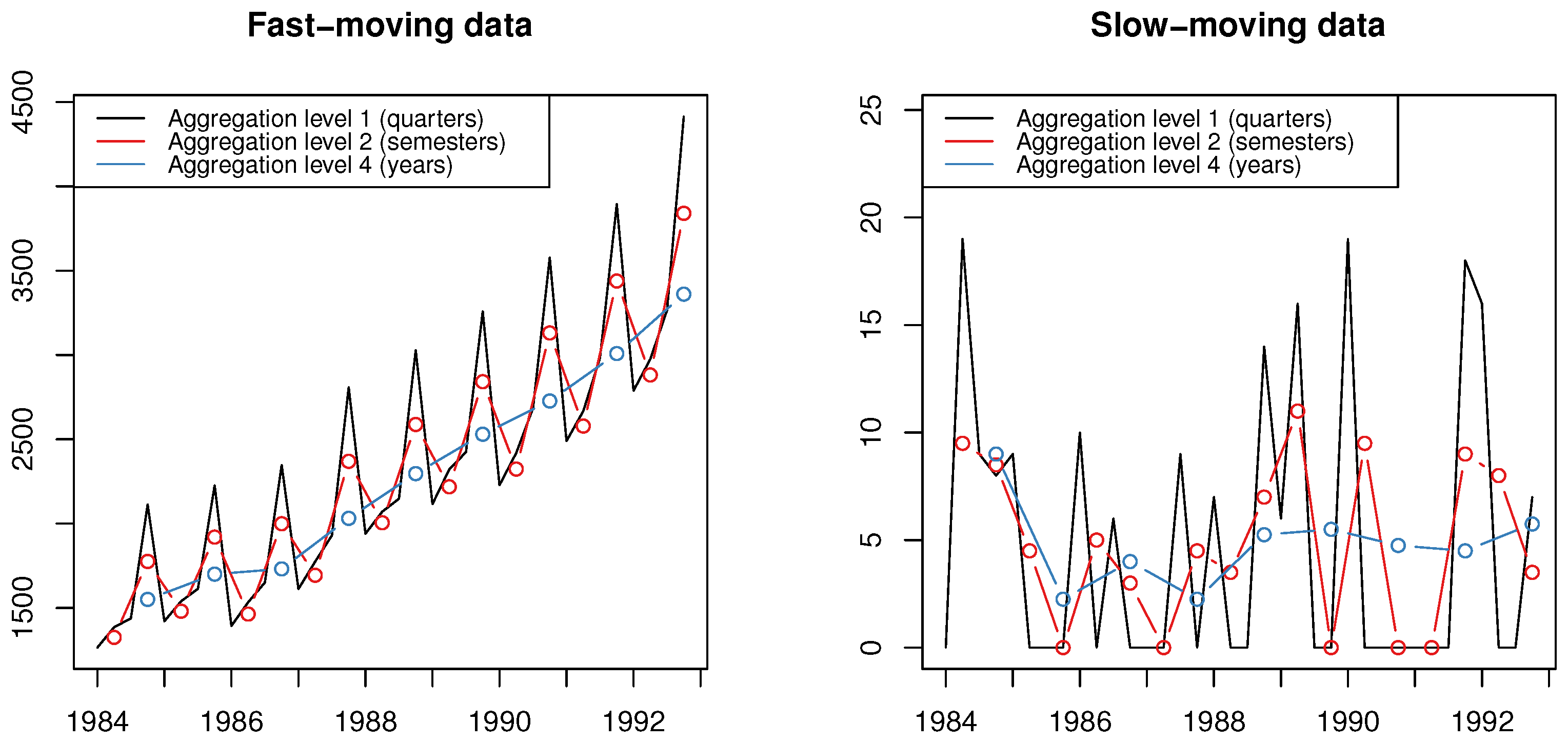
Temporal aggregation is one of the transformations that utilize the “wisdom of the data” concept to identify patterns that may be difficult to capture when analyzing the original series directly [6]. Specifically, temporal aggregation is the transformation of a time series from one frequency to another, lower frequency. For instance, a quarterly time series of length n can be transformed to a semi-yearly series of length $n/2$ by using equally sized time buckets of two periods each or a yearly series of length $n/4$ by aggregating (summing) the observations by four, as shown in Figure 1. By changing the original frequency of the data, the apparent series characteristics also change and, as a result, different patterns can be observed and modeled to produce more accurate forecasts [7]. Thus, temporal aggregation becomes relevant for predicting both slow- [8,9,10,11] and fast-moving [12,13] series. In the first case, where the data typically display intermittency or erraticness [14], the aggregation filters out randomness and reveals the underlying signal of the series. In the second case, the transformation uncovers the trend patterns of the series, while allowing seasonality and level to be modeled at different levels.

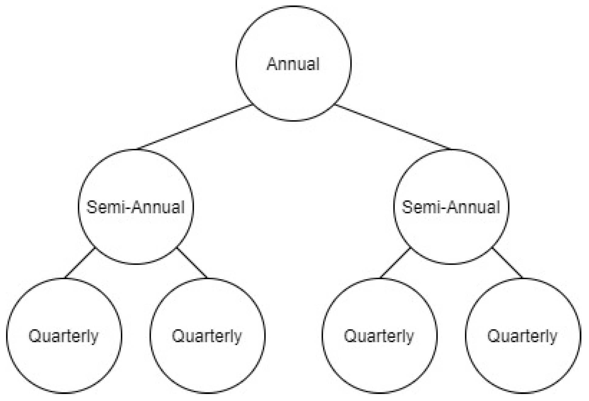
Temporal aggregation can be applied both in an non-overlapping and an overlapping manner. However, the former approach has become more popular since its results are easier to interpret and avoids introducing autocorrelations [15]. Moreover, non-overlapping aggregation allows the series created to be organized in temporal hierarchies [13] and, as a result, forecasts can be produced using methods that have been proved successful when predicting cross-sectional hierarchies. Apart for improving accuracy, forecasting with temporal hierarchies also has the advantage that it generates reconciled predictions that support aligned decisions at different planning horizons [16]. In addition, it provides a structured framework for combining forecasts from multiple temporal levels, an approach called multiple temporal aggregation.

Multiple temporal aggregation, which is effectively a forecast combination subject to linear constraints [17], has several advantages over focusing on a single aggregation level [18]. Similar to standard ensemble strategies, widely used in the literature to blend forecasts produced by different models or variants of them, it avoids selecting a single “best” aggregation level, which is challenging to do in practice [19], and mitigates model and parameter uncertainty by exploiting the merits of combining [for a non-systematic review on temporal aggregation, please refer to [6]. In practice, the main difference between standard forecast combination and multiple temporal aggregation is that in the former case, the forecasts to be ensembled are reported just at the original frequency of the series, while in the latter, they are reported at various data frequencies, thus exploiting the potential benefits of temporal aggregation in addition to those of forecast combination.

Nevertheless, multiple temporal aggregation also comes with some challenges. First, when the series is characterized by seasonality, combining seasonal base forecasts (typically produced at lower aggregation levels) with non-seasonal base forecasts (typically produced at higher aggregation levels) may lead to an unnecessary seasonal shrinkage that deteriorates accuracy. Spiliotis et al. [16] and Spiliotis et al. [20] elaborate on this issue and propose some pre-processing techniques and heuristic rules to mitigate its effect. Second, some multiple temporal aggregation methods suggest that all levels should contribute equally to the final forecasts [9], an approach that may be proved sub-optimal in practice. Simply put, the information available at some of the levels may be more critical for improving forecasting accuracy, meaning that more weight should be assigned to the respective base forecasts. Athanasopoulos et al. [13] and Wickramasuriya et al. [21] suggest accounting for error variances contributing to the forecast error at some or multiple aggregation levels to weight base forecasts more appropriately. However, these estimates still rely on in-sample one-step-ahead forecast errors (residual errors), which may neither represent post-sample performance precisely nor be correlated with the objective function ultimately used to assess forecasting performance. More importantly, these approaches will still combine the base forecasts linearly, thus possibly failing to account for complex data relationships. To tackle these issues, Jeon et al. [22] suggested using cross-validation to estimate the forecast errors and weight the base forecasts accordingly, while Spiliotis et al. [23] employed machine learning (ML) models to nonlinearly combine cross-sectional hierarchical forecasts using weights that explicitly focus on post-sample accuracy, thus allowing for more flexible and selective ensembling.

In this paper, we offer a dynamic perspective to the problem of (multiple) temporal aggregation to address the aforementioned challenges, i.e., to avoid seasonal shrinkage, dynamically compute combination weights, and adjust said weights using post-sample accuracy records. Inspired by the recent advances in the field of ML, we propose the use of a classification model to either select the most appropriate temporal aggregation level or to derive the weights that properly combine the base forecasts computed at various levels. To do so, we extract several time series features at multiple temporal aggregation levels [24] and use the features as leading indicators to estimate the importance of each level in improving forecasting accuracy. Effectively, the proposed classifier serves as a meta-learner that directly links time series features with post-sample forecasting performance. Such feature-based meta-learners have been successfully employed in the literature to combine the forecasts of multiple models [25] or predict their performance [26], but not in temporal aggregation settings.

We focus on a variant of classification trees, called LightGBM [27], that exploits the power of gradient boosting and has shown excellent performance in similar tasks [28], including time series forecasting [29]. Gradient-boosted trees are preferred over other classification models as they selectively capture nonlinear relationships across the explanatory variables (features) used for prediction, are faster to compute, have more reasonable memory requirements, are simpler to optimize in terms of hyperparameters, require less data to be sufficiently trained (e.g., compared to neural networks), and are widely used in the literature for developing meta-learners that are tasked to select or to combine forecasts from a pool of alternatives [26,30]. The contributions of this paper are threefold:

• We propose a nonlinear approach for employing (multiple) temporal aggregation and deciding either on the selection of the most suitable aggregation level for producing forecasts or on the weights to be used for combining the base forecasts of multiple levels. Compared to existing alternatives, this method is more general, relying neither on heuristic rules [8,31] nor on pre-defined weights [13,25].
• In order to analyze the complex data relationships between forecasting accuracy and time series features, we consider an ML process that involves the preparation of the data (estimation of time series features and conduction of forecasting simulations), the tuning of the meta-learner in terms of hyperparameters, and its training.
• We suggest that once the meta-learner has been trained, it can directly be used to derive the combination weights of the base forecasts for any time series at hand in a robust and fast fashion using the features of said series as input.

Note that the proposed classification model is explicitly trained with the objective of producing results that minimize the forecast error, as defined by the forecaster. More importantly, training is performed by assessing the post-sample accuracy of each forecast being combined, measured through validation. Therefore, the suggestions of the meta-learner are expected to be more representative and better match the objectives of the forecasting task at hand. In addition, given that the classifier learns from multiple time series simultaneously (cross-learning), the meta-learner generalizes better, thus avoiding biases that may occur when the forecast errors computed for deriving the combination weights are estimated for each series separately. Moreover, its results are directly linked with the characteristics of the examined series, facilitating their interpretation.

We benchmark the performance of the meta-learner against standard methods used for applying (multiple) temporal aggregation considering two large data sets that contain both fast- and slow-moving series. The benchmarks include conventional forecasting (no temporal aggregation is applied), an equally weighted combination of base forecasts [10], forecasting with temporal hierarchies [13], as well as popular time series forecasting methods that have achieved good performance in well-known forecasting competitions. The results, which include tests for significance, suggest that the proposed approach can improve forecasting accuracy, especially for the case of the fast-moving data. These improvements reach 4% when compared to conventional forecasting and about 6% when compared to popular time series forecasting methods used in the field.

The remainder of the paper is organized as follows. Section 2 describes popular methods found in the literature for applying (multiple) temporal aggregation. Section 3 presents the proposed meta-learner and explains how it can be used in practice to select or combine the base forecasts generated at various temporal aggregation levels. Section 4 presents the two data sets used for the empirical evaluation of the meta-learner and describes the experimental design. Section 5 presents our results and discusses our findings. Finally, Section 6 concludes the paper.

2. Literature Review

2.1. Temporal Aggregation

Temporal aggregation for forecasting has been extensively researched in the last two decades and may be utilized using two different approaches; either by selecting the “best” temporal aggregation level where the forecasts should be produced or by combining the forecasts produced at multiple levels in an “optimal” manner. Kourentzes et al. [19] addressed the duality of temporal aggregation, arguing that “each school of thought presents different advantages and has different limitations”.

Aggregating time series data to a certain lower frequency can become beneficial both for slow- and fast-moving series [32,33,34]. With regard to fast-moving data, Athanasopoulos et al. [35] aggregated monthly and quarterly series from the tourism industry and observed that aggregated yearly forecasts were more accurate than forecasts derived from higher frequency data. Similarly, when analysing slow-moving inventory data, Nikolopoulos et al. [8] found that forecasts produced from lower frequency data resulted in better accuracy on average.

Nevertheless, selecting the “best” aggregation level is not trivial and, as a result, no universal approach has been identified for addressing this task. For instance, Nikolopoulos et al. [8] proposed a heuristic rule corresponding to the lead time plus one review period to determine an appropriate level of aggregation for slow-moving data, while Petropoulos et al. [10] introduced a method that aggregates the original time series based on “demand buckets” instead of time windows. Another heuristic method was proposed by Spithourakis et al. [31] who approached the selection of the “best” aggregation level as an optimization problem, focusing on the minimization of in-sample forecast errors and information criteria.

2.2. Multiple Temporal Aggregation

In order to avoid selecting a single temporal aggregation level, researchers have been combining the forecasts produced at multiple levels. The multiple temporal aggregation approach has been empirically tested in many forecasting applications [12,36,37], reporting significant improvements over both simple temporal aggregation and conventional forecasting (i.e., producing forecasts at the original frequency of the series).

Even though multiple temporal aggregation can mitigate the uncertainty of selecting a single temporal aggregation level, defining the weights to be used for combining the base forecasts remains an open issue. Many approaches have been proposed to address this task [38,39,40]. Equal weights, despite their simplicity, constitute a competitive choice in many cases and there has been no proof that a more sophisticated method can consistently provide superior results [3]. However, there has been evidence that unequal weighting schemes may be more suitable for forecasting seasonal series since they can avoid unreasonable seasonal shrinkage. As a result, Kourentzes et al. [12], Spiliotis et al. [16], and Spiliotis et al. [20] proposed some alternative weighting methods for preserving the seasonal patterns of the series, while similar results can be achieved when forecasting with temporal hierarchies [13].

2.3. Temporal Hierarchies

Athanasopoulos et al. [13] introduced a novel approach on multiple temporal aggregation which resembles a hierarchical forecasting framework. The approach, called temporal hierarchies, enables the use of well-established reconciliation methods within the temporal dimension of the data, thus facilitating the combination of base forecasts, while ensuring coherence. Jeon et al. [22] used temporal hierarchies to obtain reconciled probabilistic forecasts, while Spiliotis et al. [20] proposed extensions of the framework to reduce forecast bias, avoid seasonal shrinkage, and tackle model uncertainty.

In what follows, we present a brief but complete explanation of the temporal hierarchies method as well as the alternative estimators that can be used within the framework to reconcile the base forecasts. Without loss of generality, in our discussion, we consider quarterly data (m = 4) as the temporal level at which the time series is originally observed and denote it using the m-dimensional vector $\mathbf{b}={({\mathbf{y}}_{Q_1},{\mathbf{y}}_{Q_2},{\mathbf{y}}_{Q_3},{\mathbf{y}}_{Q_4})}^{\prime }$. Semi-annual and annual data can then be constructed by using non-overlapping temporal aggregation. The temporal hierarchy in this case is structured as shown in Figure 2.

Temporal hierarchies assume that any observation at an aggregate level should be equal to the sum of the observations of its respective sub-aggregate level. Since the temporal hierarchy consists of $r=7$ nodes, the r-dimensional vector $\mathbf{y}={({\mathbf{y}}_A,{\mathbf{y}}_{S{A}_1},{\mathbf{y}}_{S{A}_2},{\mathbf{y}}_{Q_1},{\mathbf{y}}_{Q_2},{\mathbf{y}}_{Q_3},{\mathbf{y}}_{Q_4})}^{\prime }$, involving the observations of the temporally aggregated series, can be organized as follows

$$\begin{array}{c}\hfill \mathbf{y}=\mathbf{S}\mathbf{b},\end{array}$$

(1)

where

$$\begin{array}{c}\hfill \mathbf{S}=\left[\begin{array}{cccc}1& 1& 1& 1\\ 1& 1& 0& 0\\ 0& 0& 1& 1\\ & {\mathbf{I}}_m& \end{array}\right]\end{array}$$

(2)

is a “summing matrix” of order $r\times m$, while ${\mathbf{I}}_m$ is a m-dimensional identity matrix. Based on the above, reconciled forecasts can be derived by

$$\begin{array}{c}\hfill \tilde{\mathbf{y}}=\mathbf{S}\mathbf{P}\widehat{\mathbf{y}},\end{array}$$

(3)

where $\widehat{\mathbf{y}}$ are the base forecasts, $\tilde{\mathbf{y}}$ are the revised hierarchical forecasts, and $\mathbf{P}$ is a $m\times n$ matrix that combines the base forecasts. Effectively, $\mathbf{SP}$ forms a reconciliation matrix that transforms incoherent base forecasts across all aggregation levels into reconciled ones using the combinations weights defined by $\mathbf{P}$.

Note that as long as $\mathbf{P}$ has non-zero values in each column, the revised forecasts are calculated using base forecasts from all aggregation levels. Setting a column to zero will negate the effect of the corresponding level’s base forecasts. For instance, in the case of the quarterly data, if we set every column to zero except those that correspond to the quarterly base forecasts, the reconciled forecasts will be solely extracted from the bottom-level forecasts of the temporal hierarchy. Similarly, if we zero out all columns except the first, the reconciled forecasts will be solely driven by the annual base forecasts.

Wickramasuriya et al. [21] investigated the optimization of the $\mathbf{P}$ matrix, proving that if $\mathbf{W}$ is a positive definite covariance matrix of the base forecast errors, then $\mathbf{P}={\left({\mathbf{S}}^{\prime }{\mathbf{W}}^{-1}\mathbf{S}\right)}^{-1}{\mathbf{S}}^{\prime }{\mathbf{W}}^{-1}$ minimizes the $tr\left[{\mathbf{SPWP}}^{\prime }{\mathbf{S}}^{\prime }\right]$, subject to $\mathbf{SPS}=\mathbf{S}$, where ${\mathbf{SPWP}}^{\prime }{\mathbf{S}}^{\prime }=var(\mathbf{y}-\tilde{\mathbf{y}})$ is the variance covariance matrix of the h-step ahead coherent forecast errors. The method, called “MinT”, minimizes the trace of the covariance of the h-step ahead coherent forecast errors, being limited, however, by the need of knowledge of the $\mathbf{W}$ matrix.

Wickramasuriya et al. [21] and Athanasopoulos et al. [13] provided different estimators for the $\mathbf{W}$ matrix in an attempt to bypass the above mentioned limitation, as summarized below:

• Hierarchy variance scaling (${\Lambda }_H$)
  A diagonal matrix that consists of the estimates of the in-sample one-step-ahead error variances of the series that make up the hierarchy.
  In our example, that would be ${\Lambda }_H=diag{({\widehat{\sigma }}_A,{\widehat{\sigma }}_{SA1},{\widehat{\sigma }}_{SA2},{\widehat{\sigma }}_{Q1},{\widehat{\sigma }}_{Q2},{\widehat{\sigma }}_{Q3},{\widehat{\sigma }}_{Q4})}^2$.
• Series variance scaling (${\Lambda }_V$)
  A diagonal matrix that consists of estimates of the in-sample one-step-ahead error variances at each series.
  In our example, that would be ${\Lambda }_V=diag{({\widehat{\sigma }}^{\left[4\right]},{\widehat{\sigma }}^{\left[2\right]},{\widehat{\sigma }}^{\left[2\right]},{\widehat{\sigma }}^{\left[1\right]},{\widehat{\sigma }}^{\left[1\right]},{\widehat{\sigma }}^{\left[1\right]},{\widehat{\sigma }}^{\left[1\right]})}^2$.
• Structural scaling (${\Lambda }_S$)
  A diagonal matrix containing the number of forecast errors contributing to the bottom aggregation level.
  In our example, that would be ${\Lambda }_S=diag(4,2,2,1,1,1,1)$.

In conclusion, (multiple) temporal aggregation has been widely explored in the literature, but additional research is still required to effectively select the most appropriate temporal aggregation level or define the weights to be used for combining the forecasts produced at multiple levels. The selection of the “best” aggregation level is typically done using heuristic rules, while the combination of the forecasts is conducted in a linear fashion, with the combination weights being estimated based on frequency-related information or in-sample forecast errors. We argue that ML methods can be used to tackle these issues, enabling nonlinear estimations of combination weights that focus on post-sample accuracy. Moreover, we claim that the parameters of the combination scheme provided by such methods can be optimized across multiple series, thus allowing for more robust and generalized estimations.

3. Proposed Method

As discussed in Section 2, various approaches can be used to combine or to select forecasts (selection can be considered as an extreme combination case where the total weight is assigned to a single forecast and, as a result, the rest of the forecasts are discarded by receiving a weight of zero). A simple yet effective approach is to average all base forecasts available, since, due to the uncertainty present, there is often no guarantee that the “optimal” forecast combination will outperform the equal-weighted one [3]. Similarly, one may decide to combine the base forecasts using other standard operators, such as the median [41] or the mode [42], as they are less sensitive to outliers and asymmetric distributions. Nevertheless, when there is strong evidence that some forecasts are more accurate than others, forecasters usually prefer to weight the base forecasts using either linear (e.g., optimal combining and variable weighting methods) or nonlinear combination (e.g., neural network methods and self-organizing algorithms) schemes [38]. In such cases, the weights of combining are typically determined by evaluating the in-sample accuracy of the base forecasts [39,40], but cross-validation techniques [43] can also be used to better simulate their post-sample performance [1]. As a result, forecasts that are regarded as more accurate are weighted more in the combination compared to less accurate ones.

An interesting alternative to combine or to select forecasts involves the examination of the characteristics of the time series being predicted. The key idea behind this approach is that, depending on the characteristics of the series, different types of forecasts may be more relevant. Shah [44] and Meade [45] used linear regression and discriminant analysis methods to predict the performance of various forecasts, thus providing some early selection rules. Similarly, Collopy and Armstrong [46], Goodrich [47], Adya et al. [48], and Adya et al. [49] employed rule-based forecasting and expert systems to combine or to select forecasts depending on the data conditions. Petropoulos et al. [25] considered a set of time series features and the forecasting horizon to select the most appropriate forecast concluding that there are useful feature cases both for fast- and slow-moving data. More recently, Kang et al. [50] and Spiliotis et al. [51] explored the characteristics of the time series used in popular forecasting competitions, including the M3 and M4 [4], confirming that the relative performance of different forecasting methods depends on the particularities of the data.

Building on this concept, Montero-Manso et al. [30] used the M4 data set to train a meta-learner that assigned combination weights to nine different forecasting methods by linking their performance, measured through cross-validation, with the features of the series. The meta-learner, which was an extreme gradient boosted tree, was proved very successful, winning the second place in the M4 competition. Similarly, Talagala et al. [26] used a Bayesian multivariate regression method to construct a feature-based meta-leaner that predicts the performance of each forecasting method, thus providing evidence about which base forecast(s) should be selected or combined. In cross-sectional hierarchical forecasting settings, Abolghasemi et al. [28] used ML classification methods to determine, based on the characteristics of the series involved in the hierarchy, which reconciliation method (e.g., bottom-up, top-down, and optimal) should be preferred.

There are many advantages of using ML meta-learners to combine or to select forecasts over utilizing other approaches [23]. First, in contrast to expert systems and heuristic rule-based forecasting methods, the rules of the meta-learners are explicitly derived by the available data instead of being defined by experts, whose insights may be biased or focused on particular applications and data sets. Second, since ML models are nonlinear in nature, they can account for more complex relationships observed in the data compared to linear methods, also having a higher learning capacity. Third, meta-learners build their rules by directly linking time series features with post-sample performance, as defined by the forecaster, instead of considering the in-sample performance of the forecasts or accuracy measures that may differ to those actually used for the final evaluation of the forecasts, a practice that may lead to sub-optimal results [52]. Fourth, meta-learners can define the rules by observing data relationships across multiple series. As a result, the models are sufficiently generalized, avoiding biases that may occur when modeling takes place for each series separately.

Drawing from the above, we propose using a feature-based meta-learner to dynamically employ (multiple) temporal aggregation. The proposed meta-learner is a decision-tree-based classification model that can be used to either select the most appropriate temporal aggregation level or derive the weights that appropriately combine the base forecasts computed at the various levels. Below, we describe our methodological approach, including the time series features used as input by the classification model, as well as the training and forecasting process.

3.1. Feature Selection

There is a significiant range of features that can be used to describe a time series and its characteristics. When it comes to fast-moving data, a widely used set of time series features can be retrieved from the tsfeatures package for R [53]. Another interesting set of features has been introduced by Lemke and Gabrys [54], emphasizing statistics, frequency, autocorrelation, and diversity. Considering slow-moving data, Nasiri Pour et al. [55] proposed a set of features aiming to sufficiently describe lumpy series. Nevertheless, there is no objective way of determining the optimal number or set of features to be used for describing a data set, nor it is guaranteed that using the maximum amount of possible extracted features will result in better results. Therefore, in our study, we use a variety of features that, in our opinion, can sufficiently describe the essential components of the time series at hand.

Specifically, for slow-moving data, we consider two essential features that are widely used for categorizing demand patterns [56]: the average inter-demand interval (ADI), which measures the frequency of zero instances in the data set, and the coefficient of variation ($C{V}^2$), which measures the variation of non-zero demand occurrences. In addition, we use some of the features proposed by Nasiri Pour et al. [55]. Note that the aforementioned features are calculated both for the original time series and the time series of lower frequencies derived when employing temporal aggregation. This process results in a richer set of features that not only describes the original data set, but also provides useful information for the temporally aggregated series.

With regard to the fast-moving data, we exploit the wide variety of features provided by the tsfeatures package. The features capture time series characteristics such as trend, seasonality, and stability, as well as statistical measures over the time series data, such as autocorrelation. In resemblance to the approach used for the slow-moving data, we extract the selected features at all temporal aggregation levels. The features used, along with the levels on which they are calculated for both the slow- and fast-moving data sets, are presented in

Table A1. Features used for the slow-moving series (M5 competition data set).

No.	Feature Description	B01	B07	B14	B28
1	Average inter-demand interval (ADI)	✓	✓	✓	✓
2	Coefficient of variation of the demand when it occurs (${\mathrm{CV}}^2$)	✓	✓	✓	✓
3	Number of periods separating the last two nonzero demand occurrences as of the end of the immediately preceding target period	✓	✗	✗	✗
4	Maximum number of consecutive zeros between two non-zero demands	✓	✗	✗	✗
5	Number of consecutive periods with demand occurrence, immediately preceding target period	✗	✓	✓	✓
6	Average demand among seven periods immediately preceding the target period	✓	✓	✓	✓
7	Maximum demand among seven periods immediately preceding the target period	✓	✓	✓	✓

and

Table A2. Features used for the fast-moving series (M4 competition data set).

No.	Feature	Feature Description	B01	B02	B03	B04	B06	B12
1	seasonality	Strength of seasonality	✓	✓	✓	✓	✓	✗
2	entropy	Spectral (Shannon) entropy	✓	✓	✓	✓	✓	✗
3	trend	Strength of trend	✓	✓	✓	✓	✓	✓
4	linearity	The linearity of the series based on the coefficients of an orthogonal quadratic regression	✓	✓	✓	✓	✓	✓
5	x_acf1	Autocorrelation coefficient at the first lag	✓	✓	✓	✓	✓	✓
6	seas_pacf	Seasonal partial autocorrelation of the series	✓	✓	✓	✓	✓	✗
7	seas_acf1	Autocorrelation coefficient at the first seasonal lag	✓	✓	✓	✓	✓	✗
8	diff1_acf1	Autocorrelation coefficient at the first lag of the differenced series	✓	✓	✗	✗	✗	✗
9	diff2_acf1	Autocorrelation coefficient at the first lag of the twice-differenced series	✓	✓	✗	✗	✗	✗
10	diff2_acf10	The sum of squares of the first 10 autocorrelation coefficients of the twice-differenced series	✓	✓	✗	✗	✗	✗
11	e_acf1	The first autocorrelation coefficient of $e_t$	✓	✓	✓	✓	✓	✗
12	curvature	The curvature of the series based on the coefficients of an orthogonal quadratic regression.	✓	✓	✓	✓	✓	✗
13	lumpiness	The variance of the variances calculated on tiled (non-overlapping) windows	✓	✓	✓	✓	✓	✓
14	stability	The variance of the means calculated on tiled (non-overlapping) windows	✓	✓	✓	✓	✓	✓
15	nonlinearity	The nonlinearity coefficient of the series	✓	✓	✓	✓	✗	✓
16	hw_alpha	The smoothing parameter of an additive seasonal trend model implemented on the series	✓	✓	✓	✓	✓	✗

of Appendix A.

3.2. Classifier (Meta-Learner)

In the attempt to develop a meta-learner, we utilize a ML classification model. Classification consists a supervised ML problem, focusing on the accurate assignment of observations (in our case, time series) into certain classes (in our case, temporal aggregation levels). The problem can be either binary, meaning that there are only two possible classes, or multi-class.

To perform classification, a set of selected features (inputs) is extracted for each observation included in the data set used for training the ML method, along with their respective class (output or label). Then, the method is tasked to identify patterns so that the classes are precisely predicted based on the features available. Ultimately, once the relationships between the classes and the features have been learned, the method can be used to classify observations that were not originally included in the train set. Note that most classifiers do not predict the label per se, but estimate the probability of a class to be the “right” one. Therefore, the output of the classifier can be realized as a probabilistic prediction that can be used to identify the class that is presumably “correct”.

In the settings of our study, the probabilities will refer to how likely it is for a certain temporal aggregation level to result in the most accurate forecasts. Consequently, selecting the level of the highest probability will suggest forecasting through temporal aggregation, while combing the forecasts produced at all levels with weights that are driven by said probabilities will suggest forecasting through multiple temporal aggregation. Note that, if the lowest temporal aggregation level is identified as “best”, the classifier will effectively suggest conventional forecasting, i.e., forecasting at the original frequency of the series.

Although the classifier can be implemented using any ML model of preference, we chose a gradient boosting model due to its high accuracy and low computational cost. Specifically, we employed the Booster model from the LightGBM library for Python, an ML algorithm built on gradient boosting trees that generates multiple independent trees, one at a time, aiming to decrease each time the errors made by the former trained tree.

LightGBM involves several hyperparameters that can significantly affect its performance. In order to tune them, we apply grid search, an automated method that explores a set of different hyperparameter values and computes the forecasting performance on a validation set to find the most appropriate ones, as defined by an accuracy measure. We focus on the most critical hyperparameters, i.e., the number of boosting iterations ($N_{iterations}$), which determines the number of trees to be created (the model generates ($N_{labels}$ × $N_{iterations}$) trees), the maximum number of leaves in each tree ($N_{leaves}$), the learning rate, the percentage of features sampled (feature fraction), the percentage of data sampled from the data set without re-sampling (bagging fraction), and the frequency in which the data are being sampled during the iterations (sampling frequency).

The ranges from which the hyperparameter values were randomly sampled in our experiments are presented in

Table 1. Hyperparameters ranges for validation process.

Hyperparameter	Range
$N_{iterations}$	[10, 150]
$N_{leaves}$	[10, 200]
$LearningRate$	(0, 1)
$FeatureFraction$	(0, 1]
$BaggingFraction$	(0, 1]
$SamplingFrequency$	[10, 100]

. In our case, the validation set consisted of the last h observations of the time series train set, with h being the forecasting horizon. However, once the hyperparameters were identified, the classifier was re-trained using the complete train set.

3.3. Forecasting Framework

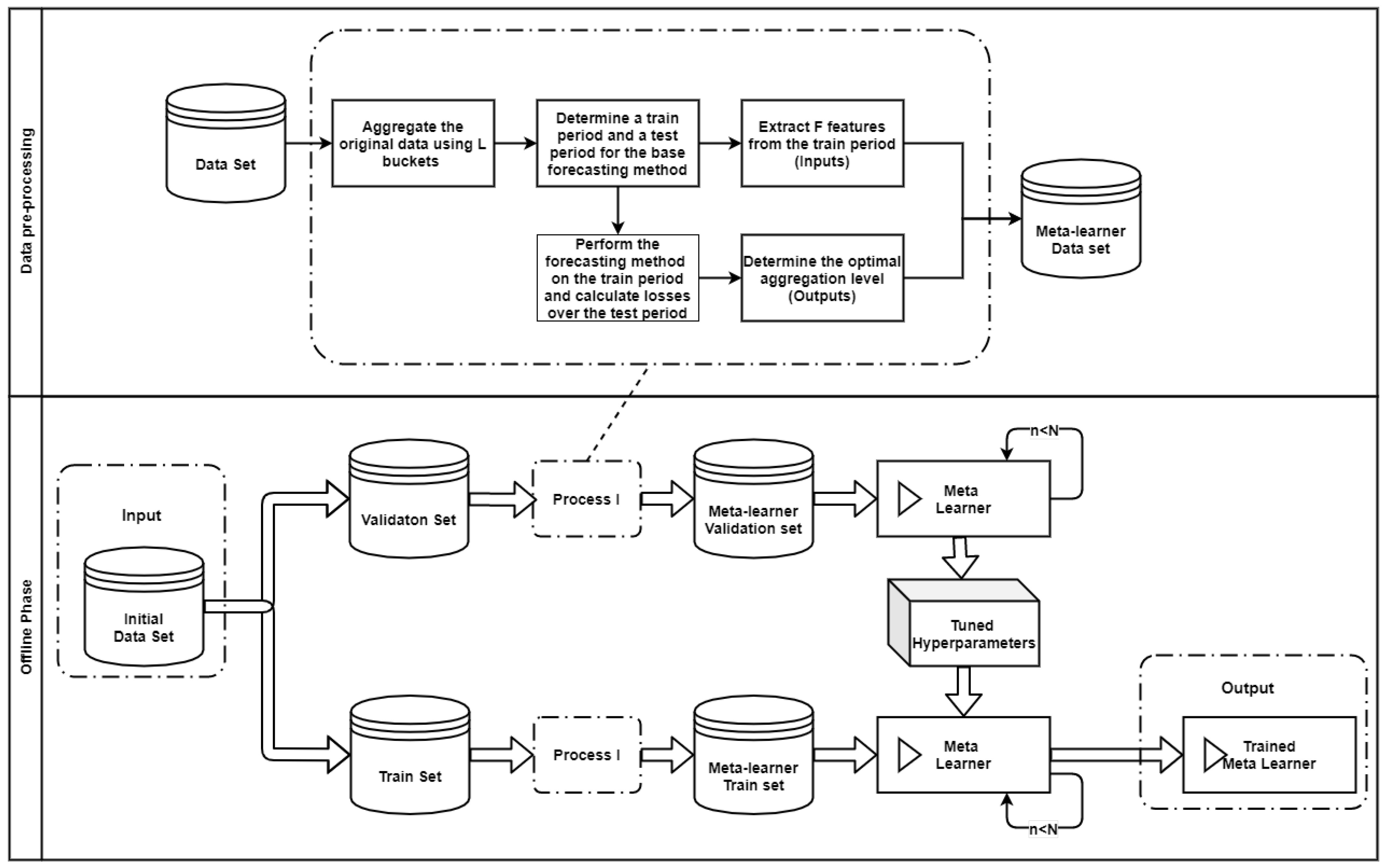
The proposed framework, summarized in Algorithm 1, is implemented into two phases; the offline and the online phase. The offline phase involves the preparation of the data, the tuning of the meta-learner, and the training process, while the online phase puts in actual use the trained classifier to generate forecasts. The pipeline for implementing the framework is also visualized in Appendix B.

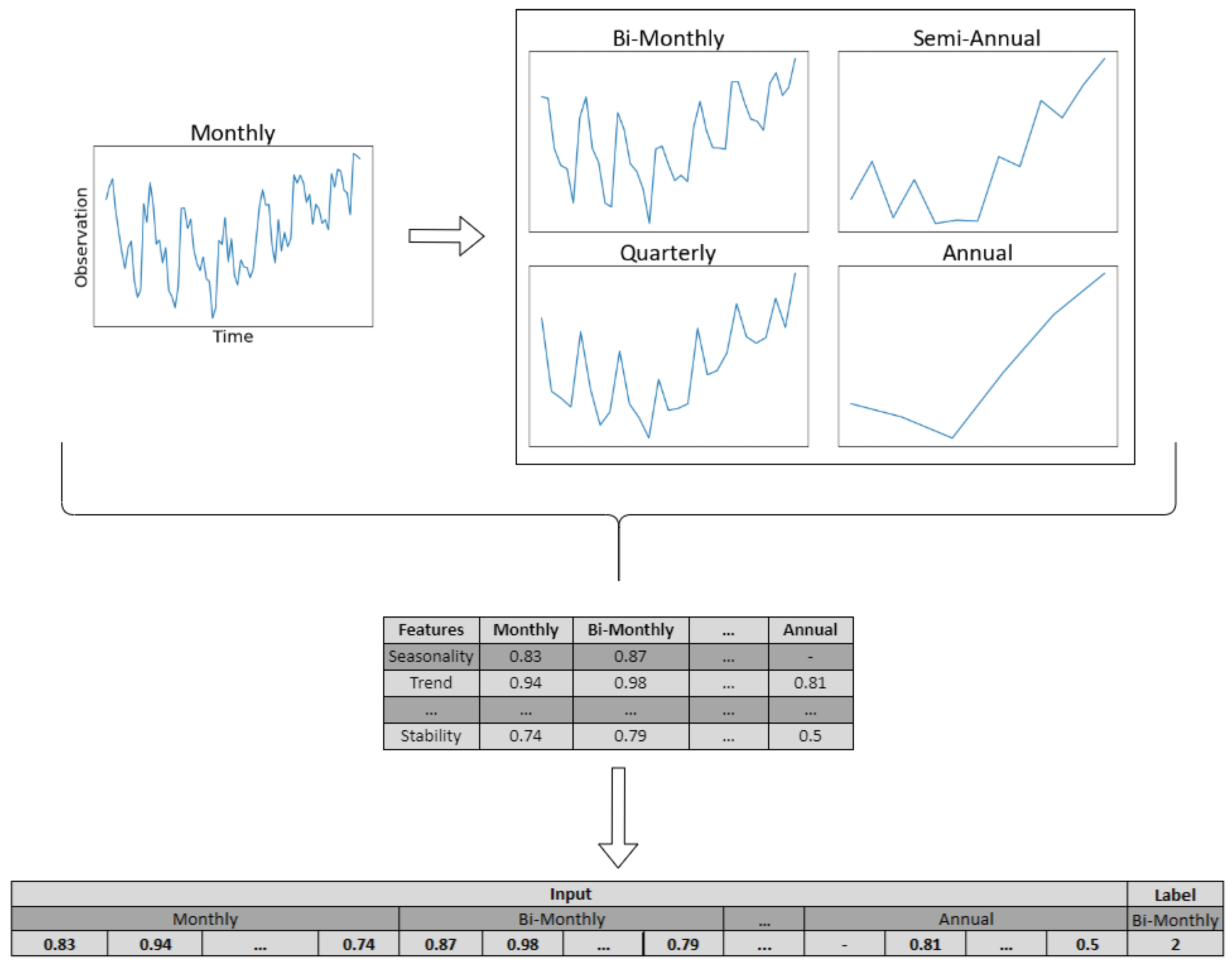
The first objective of the framework is to select for each time series of a given data set the most suitable level of temporal aggregation, i.e., the level that maximizes forecasting accuracy. Given a time series of certain frequency, we employ non-overlapping temporal aggregation to transform the data into lower frequencies. From the constructed time series, and depending on whether the data are slow- or fast-moving, we extract the time series features presented in Section 3.1. Then, base forecasts are computed for each aggregation level using a forecasting method of preference. Finally, given a validation set, the forecasts are evaluated using an error measure of choice and the aggregation level that reports the highest accuracy is labeled as the “right” class. The aforementioned process is repeated for all the series included in the data set, resulting in a rich set of time series features and their corresponding “best” level of temporal aggregation. An illustrative example of the data set preparation stage is presented in Figure 3 for a monthly time series. Having the train set of the meta-learner constructed, we tune the hyperparameters of the classifier as described in Section 3.2 and then train the model using the complete train set. These steps complete the offline phase of the framework.

Algorithm 1: Forecasting with conditional (multiple) temporal aggregation

After training the meta-learner, we move on to the online phase of the framework in which the meta-learner predicts the “best” aggregation level(s) of a given time series. To do so, we introduce two methods for combining the base forecasts, using as input the probabilities generated by the classifier for each level.

3.3.1. Probability-Based Weights

Let p = $[p_1,p_2,...,p_L]$ be a probability vector, where L is the number of examined temporal aggregation levels and $p_i$ the probability that the i-th level will result to the most accurate forecasts. Then, the combination weight for the corresponding forecasts will be

$$\begin{array}{cc}\hfill w_i& =\frac{p_i^2}{{\sum }_{j=1}^L{p}_j^2}.\hfill \end{array}$$

(4)

If we denote the forecasts of the i-th aggregation level as $y_i$, then the forecast of the ensemble $\widehat{y}$ will be

$$\begin{array}{cc}\hfill \widehat{y}& =\sum _{i=1}^L{w}_i\times {\widehat{y}}_i.\hfill \end{array}$$

(5)

Note that since in Equation (4), the probabilities are squared, the weights assigned to temporal aggregation levels of relatively low probabilities will further decrease, while levels of relatively high probabilities will retain a significant impact on the final forecasts. As a result, the negative effect of presumably inaccurate forecasts is reduced.

3.3.2. Probability-Based Structural Scaling

This approach utilizes the structural scaling estimator of the temporal hierarchies, using, however, a modified version of the ${\Lambda }_S$ matrix so that, similarly to our previous approach, the contribution of the presumably inaccurate forecasts to the ensemble is shrinked.

We approximate the W matrix as ${\Lambda }_Q=diag(Q_1,Q_2,...,Q_L)$, with L being the number of aggregation levels (in the case of quarterly data, $L=3$). Each value of the diagonal of the ${\Lambda }_Q$ matrix is then calculated as

$$\begin{array}{cc}\hfill {\mathbf{Q}}_i& =\mathbf{S}{\mathbf{I}}_{f_i}\frac{(1-p_i)}{(L-1)f_i},i\in [1,L],\hfill \end{array}$$

(6)

where $f_i$ is the data frequency of the i-th level, ${\mathbf{I}}_{f_i}$ is a $f_i$-dimensional identity matrix, and $p_i$ is the probability appointed by the classifier to the i-th level.

4. Empirical Evaluation

4.1. Data Sets

To evaluate the performance of the proposed approach both for the case of fast- and slow-moving data, we consider two different data sets that are widely used in the forecasting literature for benchmarking. The first data set includes the monthly series of the M4 competition [4], while the second the daily product-store series of the M5 competition [29].

The M4 competition involves 48,000 monthly time series that originate from several domains, namely microeconomic, industry, macroeconomic, finance, demographic, and others. Moreover, compared to other public data sets, the competition consists of diverse series that sufficiently represent several real-world forecasting applications [51]. The lengths of the series differ, ranging from 5 to about 82 years, with the majority of the series covering a period of about 18 years. Note that M4 originally involved the prediction of 100,000 time series that covered in addition to the monthly series, yearly, quarterly, weekly, daily, and hourly data. Our choice to focus on the monthly data of the competition is twofold. First, temporal aggregation becomes more meaningful for series of relatively high frequencies. The lower the frequency, the fewer the temporal aggregation levels that can be constructed and used by the meta-learner to improve forecasting accuracy. For instance, yearly data cannot be meaningfully aggregated further, while quarterly data can construct just three temporal levels (quarterly, semi-yearly, and yearly data), in contrast to monthly that can construct six temporal levels (monthly, bi-monthly, quarterly, four-monthly, semi-yearly, and yearly data). Second, the weekly, daily, and hourly series of the M4 competition were considerably fewer in number compared to the monthly data, thus limiting the learning potential of the proposed meta-learner and the significance of our results.

The M5 competition involves 30,490 time series that represent the hierarchical unit sales of the largest retail company in the world, Walmart. Specifically, the series cover 3490 products, which can be classified into three product categories (hobbies, foods, and household), sold across 10 stores, located in the states of California, Texas, and Wisconsin. The series are daily and cover a period of about 5.5 years, but their lengths differ, ranging from 124 to 1969 days (about 1810 days on average). According to Spiliotis et al. [51], 73% of the series are intermittent, 17% are lumpy, 3% are erratic, and 7% are smooth [14]. This makes M5 a representative data set for evaluating the performance of the proposed approach on slow-moving series. Moreover, Theodorou et al. [24] suggest that the M5 data sufficiently represent retailers that operate in different regions, sell different product types, and consider different marketing strategies than Walmart. Thus, we expect our results to be relevant for various retail firms around the globe.

Both data sets are publicly available and can be downloaded from the GitHub repository (https://github.com/Mcompetitions, accessed on 10 April 2023) devoted to the M competitions.

4.2. Experimental Design

Our experimental design closely follows the original setup of each competition. In this regard, in the M4 data set we consider a forecasting horizon of 1.5 years, using the last 18 months as a test set and the rest of the observations for validation and training, i.e., for defining the values of the hyperparameters to be used by the meta-leaner and estimating the model accordingly. Similarly, in the M5 data set, we use the last 28 days as a test set and the previous observations for training and validation.

In the M4 data set, forecasting accuracy is measured using the mean absolute scaled error (MASE; [57]), defined as follows:

$$\begin{array}{c}\hfill \mathrm{MASE}=\frac{1}{h}\frac{{\displaystyle \sum _{t=n+1}^{n+h}|y_t-{\widehat{y}}_t|}}{{\displaystyle \frac{1}{n-m}\sum _{t=m+1}^n|y_t-y_{t-m}|}},\end{array}$$

where $y_t$ is the actual observation of the series at period t, ${\widehat{y}}_t$ is the respective forecast, h is the forecasting horizon, n is the number of the in-sample observations (data points available in the train set), and m is the number of periods within a seasonal cycle (e.g., $m=12$ for monthly data). The values of MASE are averaged across different time series to estimate overall accuracy. Lower MASE values suggest better forecasts.

MASE is independent of the scale of the data, has a predictable behavior, has a defined mean and a finite variance, and is symmetric in the sense that it penalizes equally positive and negative forecast errors, as well as large and small ones. Therefore, it is preferred over other popular accuracy measures, such as relative or percentage errors. Moreover, MASE was one of the two measures used in M4 for evaluating the methods originally submitted in the competition.

In a similar fashion, in the M5 data set, we measure accuracy using the root mean squared scaled error (RMSSE), defined as follows:

$$\begin{array}{c}\hfill \mathrm{RMSSE}=\sqrt{\frac{1}{h}\frac{{\displaystyle \sum _{t=n+1}^{n+h}{\left(y_t-{\widehat{y}}_t\right)}^2}}{{\displaystyle \frac{1}{n-m}\sum _{t=m+1}^n{(y_t-y_{t-m})}^2}}}.\end{array}$$

RMSSE shares the same properties as MASE, but is more suitable for data that display intermittency. This is because squared errors are optimized for the mean of the data [58] instead of the median [59]. Therefore, methods that report lower RMSSE values will identify more accurately the expected demand, avoiding putting too much focus on zero sales. Additionally, this measure is consistent to the one originally used in M5 for evaluating the accuracy of the submitted methods.

The validation of the proposed meta-learner took place using the 18 and 28 observations preceding the test sets of the M4 and M5 data sets, respectively. As explained in Section 3.3, various sets of hyperparameter values were considered, and the top-performing one on the validation set was selected per case to train the meta-learner. The selected hyperparameter values are presented in

Table 2. Selected hyperparameter values of the meta-learner for the fast-moving (M4) and slow-moving (M5) data sets.

Hyperparameter	Fast-Moving (M4)	Slow-Moving (M5)
Number of iterations	12	135
Number of trees	720	540
Learning rate	0.89	0.10
Number of leaves per tree	86	23
Feature fraction	95.5%	94.5%
Bagging fraction	80.0%	88.0%
Bagging frequency	22	25

.

Note that the monthly series of the fast-moving data set can be naturally aggregated at six different levels to form a meaningful temporal hierarchy, considering buckets of 1 (month), 2 (bi-month), 3 (quarter), 4 (four months), 6 (semi-year), and 12 (year) observations. The same is not true for the daily series of the slow-moving data set since different months may consist of a different number of days. In this respect, we considered four temporal levels using buckets of 1 (day), 7 (week), 14 (two weeks or about half a month), and 28 observations (four weeks or about a month) that offer a reasonable temporal hierarchy. As a result, the classifier of the meta-learner will be trained in the M4 and M5 data sets by considering six and four aggregation levels as labels, respectively.

4.3. Base Forecasts

We produce base forecasts using the exponential smoothing family of models, as proposed by Hyndman et al. [60] and implemented in the forecast package for R [61].

Exponential smoothing is a univariate forecasting method that extrapolates series by smoothing the historical data and assuming that the most recent observations available are the most relevant for predicting the future ones. Depending on the model, exponential smoothing may account just for the level of the series or handle trend and seasonality. Therefore, the ETS (error, trend, seasonality) framework, which involves a total of 30 exponential smoothing models and selects the best one based on information criteria, is an ideal method for automatically producing forecasts at multiple temporal aggregation levels, each having different time series features.

Since exponential smoothing forecasts are intuitive, fast to compute, and accurate compared to other methods, the method has become popular in the industry and forecasting literature, being the standard method of choice in numerous forecasting applications [6]. Moreover, exponential smoothing has been one of the most accurate benchmarks considered in the M4 and M5 competitions, outperforming many of the participating teams.

5. Results and Discussion

The forecasting performance of the meta-learner in the M4 and M5 data sets is summarized in

Table 3. Forecasting performance of the proposed method in the M4 (fast-moving data) and M5 (slow-moving data) series. MASE and RMSSE are used to measure accuracy in each set, respectively. The accuracy of the examined benchmarks is also reported to enable comparisons.

	Fast-Moving (M4)		Slow-Moving (M5)
Method	MASE	Rank	RMSSE	Rank
	Benchmarks
CON	0.9478	5	0.7761	6
CON(Comb/${\mathrm{Com}}_{\mathrm{b}}$)	0.9662	7	0.7912	8
CON(Theta/SBA)	0.9695	8	0.7864	7
MTA-EW	0.9623	6	0.7716	4
MTA-STR	0.9199	3	0.7712	3
	Conditional (multiple) temporal aggregation
CTA	0.9444	4	0.7746	5
CMTA-PW	0.9136	1	0.7709	1
CMTA-PSTR	0.9186	2	0.7711	2

. CTA stands for conditional temporal aggregation, where a single “best” level is selected by the meta-learner, CMTA-PW for conditional multiple temporal aggregation with probability-based weights, and CMTA-PSTR for conditional multiple temporal aggregation with probability-based structural scaling. In all cases, ETS is used for producing the base forecasts.

To enable comparisons, we also consider several benchmarks. The first benchmark, CON, refers to conventional forecasting, i.e., producing forecasts only at the original frequency of the series using ETS. The second, MTA-EW, is a simple implementation of multiple temporal aggregation where the base ETS forecasts are combined using equal weights. The third benchmark, MTA-STR, involves forecasting with temporal hierarchies, using the ETS framework and the structural scaling matrix as estimator. In addition, to allow comparisons with popular time series forecasting methods, we include two more benchmarks per data set, namely the top performing approaches from the benchmarks considered by the organizers of the M4 and M5 competitions. For M4, this is the simple arithmetic average of SES, Holt, and Damped exponential smoothing (Comb) and the Theta method [62], while for M5, this is the simple arithmetic mean of ETS and ARIMA (${\mathrm{Com}}_{\mathrm{b}}$) and the Syntetos–Boylan approximation (SBA; [14]). Note that Comb, ${\mathrm{Com}}_{\mathrm{b}}$, Theta, and SBA represent conventional forecasting approaches.

The results of Table 3 suggest that, in both data sets, the meta-learner outperforms the rest of the forecasting approaches when used for applying multiple temporal aggregation. CMTA-PW is slightly more accurate than CMTA-PSTR, but the differences between the two combination methods are minor. Despite the uncertainty involved in the selection process, CTA also results in slightly more accurate forecasts than CON, being at the same time better than MTA-EW in the M4 data set. Moreover, we observe that the proposed meta-learners always outperform the Comb/${\mathrm{Com}}_{\mathrm{b}}$ and Theta/SBA methods. This finding is encouraging, highlighting the potential benefits of the proposed method over traditional approaches where temporal aggregation is either neglected or implemented without investigating the contribution of each temporal aggregation level to the final forecasts.

Our results are in agreement with the literature, confirming that multiple temporal aggregation can improve the accuracy of conventional forecasting, also being more effective in general than simple temporal aggregation. This conclusion remains true when reviewing both the benchmarks and the variants of the proposed meta-learner.

Another important finding refers to the extent of the accuracy improvements depending on the particularities of the data set. As seen in Table 3, multiple temporal aggregation is more effective in fast-moving data than in slow-moving series. This can be attributed to the variation and intermittency of the M5 data that render the extraction of time series patterns more challenging, even at high aggregation levels. In contrast, temporal aggregation manages to extract hidden patterns in the M4 data, where the series are less noisy and are characterized by trend and seasonality.

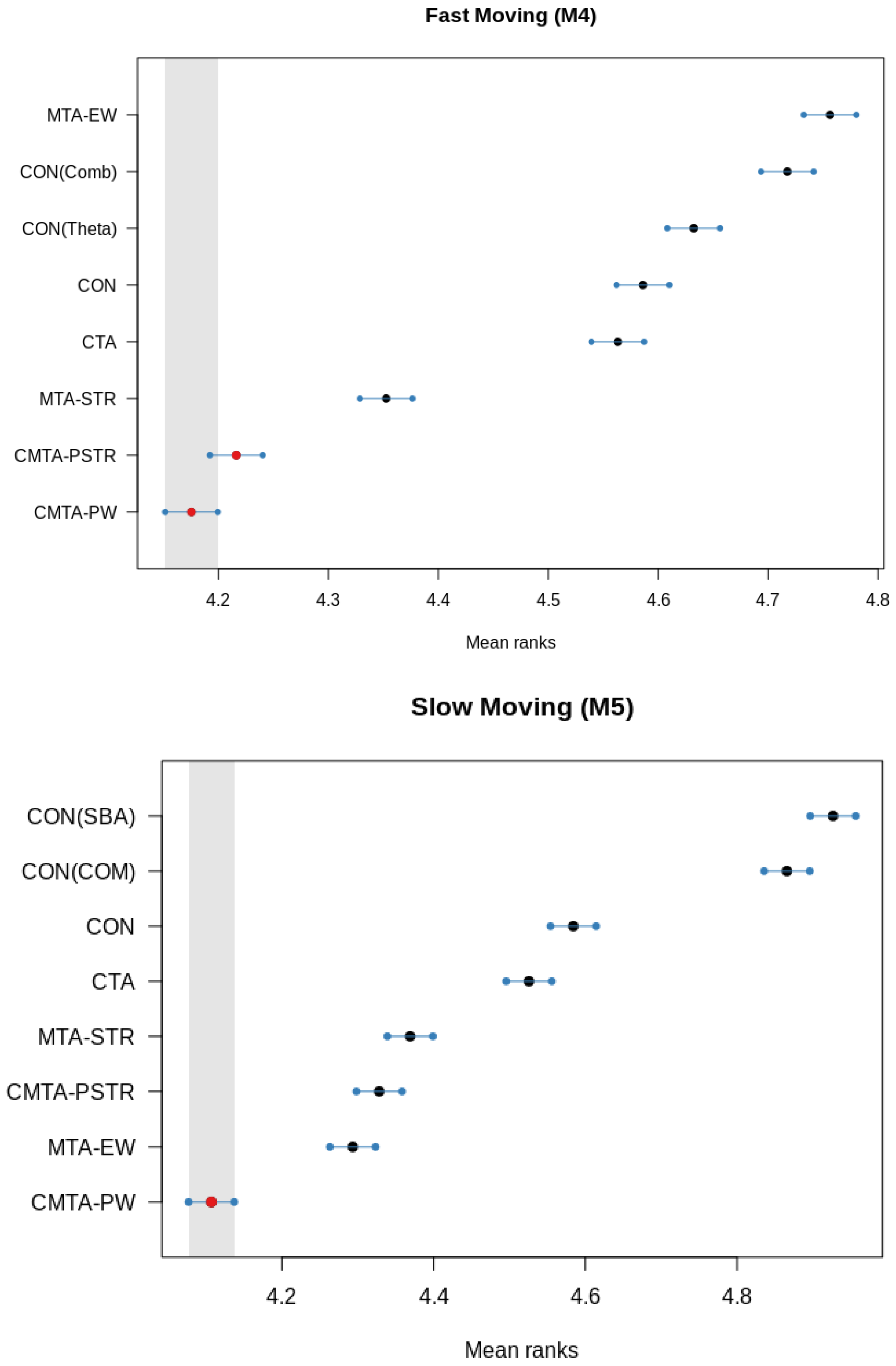
In order to obtain a better understanding of the differences of the examined forecasting approaches, we apply the multiple comparisons with the best (MCB) test that compares whether the average ranking of a forecasting method is significantly better or worse than the other methods [63]. The results are shown in Figure 4. If the intervals of two methods do not overlap, this indicates a statistically different performance. Thus, methods that do not overlap with the gray interval of the figures are considered significantly worse than the best method, and vice versa.

Focusing on the fast-moving series, it is confirmed that conditional multiple temporal aggregation significantly outperforms the rest of the methods, with CMTA-PW and CMTA-PSTR being, however, of similar accuracy. MTA-STR follows in terms of average rank, being significantly more accurate than CTA and CON. Interestingly, MTA-EW has the lowest performance, possibly due to the seasonal shrinkage it implies. Regarding the slow-moving data, CMTA-PW is again the top-ranked method and significantly better than the rest of the forecasting approaches. However, in this case it is followed by MTA-EW, which is reasonable given the lack of strong seasonal patterns in the M5 data set. Yet, MTA-EW is not significantly better than the approaches that build on structural scaling, being superior only to conventional forecasting and CTA. We also observe that in both data sets, CON has a better average rank than the Comb/${\mathrm{Com}}_{\mathrm{b}}$ and Theta/SBA forecasting approaches. Therefore, we conclude that ETS has been correctly identified as the most accurate method for producing base forecasts, enhancing the performance of the methods considered for applying (multiple) temporal aggregation.

6. Conclusions

We have proposed a meta-learner that can be used to either select the most appropriate temporal aggregation level for producing forecasts or to derive weights that properly combine the forecasts generated at various levels. To do so, the meta-learner extracts a rich set of time series features and correlates them to post-sample forecasting accuracy, thus allowing for conditional forecast selection or combination.

Our results indicate that conditional (multiple) temporal aggregation can outperform both conventional forecasting and established methods used for applying temporal aggregation. The improvements are more significant for fast-moving data where patterns are easier to identify, but can be realized for slow-moving data as well. As expected, conditional multiple temporal aggregation performs better on average than conditional temporal aggregation. However, we find that in many cases, selecting the “best” aggregation level is feasible, leading to better forecasts than forecasting at the original data frequency.

Future work could focus on extending and improving the proposed approach. This could include the investigation of alternative classification methods (e.g., logistic regression, extreme gradient boosting, and neural networks) and the development of alternative schemes for transforming classification probabilities into combination weights. Moreover, since the potential benefits of (multiple) temporal aggregation seem to magnify for time series of relatively higher frequencies, the proposed meta-learner could be tested for data that are sampled on an hourly or even minute basis. To the best of our knowledge, the work performed in the field of temporal aggregation has insufficiently covered said applications, despite the fact that methods such as the one proposed in the present paper could improve forecasting accuracy through a conditional aggregation of time series patterns observed at different temporal aggregation levels.

References

1. Fildes, R.; Petropoulos, F. Simple versus complex selection rules for forecasting many time series. J. Bus. Res. 2015, 68, 1692–1701. [Google Scholar] [CrossRef] [Green Version]
2. Petropoulos, F.; Hyndman, R.J.; Bergmeir, C. Exploring the sources of uncertainty: Why does bagging for time series forecasting work? Eur. J. Oper. Res. 2018, 268, 545–554. [Google Scholar] [CrossRef]
3. Claeskens, G.; Magnus, J.R.; Vasnev, A.L.; Wang, W. The forecast combination puzzle: A simple theoretical explanation. Int. J. Forecast. 2016, 32, 754–762. [Google Scholar] [CrossRef] [Green Version]
4. Makridakis, S.; Spiliotis, E.; Assimakopoulos, V. The M4 Competition: 100,000 time series and 61 forecasting methods. Int. J. Forecast. 2020, 36, 54–74. [Google Scholar] [CrossRef]
5. Petropoulos, F.; Spiliotis, E. The Wisdom of the Data: Getting the Most Out of Univariate Time Series Forecasting. Forecasting 2021, 3, 478–497. [Google Scholar] [CrossRef]
6. Petropoulos, F.; Apiletti, D.; Assimakopoulos, V.; Babai, M.Z.; Barrow, D.K.; Ben Taieb, S.; Bergmeir, C.; Bessa, R.J.; Bijak, J.; Boylan, J.E.; et al. Forecasting: Theory and practice. Int. J. Forecast. 2022, 38, 705–871. [Google Scholar] [CrossRef]
7. Panagiotelis, A.; Athanasopoulos, G.; Gamakumara, P.; Hyndman, R.J. Forecast reconciliation: A geometric view with new insights on bias correction. Int. J. Forecast. 2021, 37, 343–359. [Google Scholar] [CrossRef]
8. Nikolopoulos, K.; Syntetos, A.A.; Boylan, J.E.; Petropoulos, F.; Assimakopoulos, V. An aggregate–disaggregate intermittent demand approach (ADIDA) to forecasting: An empirical proposition and analysis. J. Oper. Res. Soc. 2011, 62, 544–554. [Google Scholar] [CrossRef] [Green Version]
9. Petropoulos, F.; Kourentzes, N. Forecast combinations for intermittent demand. J. Oper. Res. Soc. 2015, 66, 914–924. [Google Scholar] [CrossRef] [Green Version]
10. Petropoulos, F.; Kourentzes, N.; Nikolopoulos, K. Another look at estimators for intermittent demand. Int. J. Prod. Econ. 2016, 181, 154–161. [Google Scholar] [CrossRef] [Green Version]
11. Kourentzes, N.; Athanasopoulos, G. Elucidate structure in intermittent demand series. Eur. J. Oper. Res. 2021, 288, 141–152. [Google Scholar] [CrossRef]
12. Kourentzes, N.; Petropoulos, F.; Trapero, J.R. Improving forecasting by estimating time series structural components across multiple frequencies. Int. J. Forecast. 2014, 30, 291–302. [Google Scholar] [CrossRef] [Green Version]
13. Athanasopoulos, G.; Hyndman, R.J.; Kourentzes, N.; Petropoulos, F. Forecasting with temporal hierarchies. Eur. J. Oper. Res. 2017, 262, 60–74. [Google Scholar] [CrossRef] [Green Version]
14. Syntetos, A.A.; Boylan, J.E. The accuracy of intermittent demand estimates. Int. J. Forecast. 2005, 21, 303–314. [Google Scholar] [CrossRef]
15. Boylan, J.E.; Babai, M.Z. On the performance of overlapping and non-overlapping temporal demand aggregation approaches. Int. J. Prod. Econ. 2016, 181, 136–144. [Google Scholar] [CrossRef] [Green Version]
16. Spiliotis, E.; Petropoulos, F.; Kourentzes, N.; Assimakopoulos, V. Cross-temporal aggregation: Improving the forecast accuracy of hierarchical electricity consumption. Appl. Energy 2020, 261, 114339. [Google Scholar] [CrossRef]
17. Hollyman, R.; Petropoulos, F.; Tipping, M.E. Understanding forecast reconciliation. Eur. J. Oper. Res. 2021, 294, 149–160. [Google Scholar] [CrossRef]
18. Andrawis, R.R.; Atiya, A.F.; El-Shishiny, H. Combination of long term and short term forecasts, with application to tourism demand forecasting. Int. J. Forecast. 2011, 27, 870–886. [Google Scholar] [CrossRef]
19. Kourentzes, N.; Rostami-Tabar, B.; Barrow, D.K. Demand forecasting by temporal aggregation: Using optimal or multiple aggregation levels? J. Bus. Res. 2017, 78, 1–9. [Google Scholar] [CrossRef] [Green Version]
20. Spiliotis, E.; Petropoulos, F.; Assimakopoulos, V. Improving the forecasting performance of temporal hierarchies. PLoS ONE 2019, 14, e0223422. [Google Scholar] [CrossRef] [Green Version]
21. Wickramasuriya, S.L.; Athanasopoulos, G.; Hyndman, R.J. Optimal Forecast Reconciliation for Hierarchical and Grouped Time Series Through Trace Minimization. J. Am. Stat. Assoc. 2019, 114, 804–819. [Google Scholar] [CrossRef]
22. Jeon, J.; Panagiotelis, A.; Petropoulos, F. Probabilistic forecast reconciliation with applications to wind power and electric load. Eur. J. Oper. Res. 2019, 279, 364–379. [Google Scholar] [CrossRef]
23. Spiliotis, E.; Abolghasemi, M.; Hyndman, R.J.; Petropoulos, F.; Assimakopoulos, V. Hierarchical forecast reconciliation with machine learning. Appl. Soft Comput. 2021, 112, 107756. [Google Scholar] [CrossRef]
24. Theodorou, E.; Wang, S.; Kang, Y.; Spiliotis, E.; Makridakis, S.; Assimakopoulos, V. Exploring the representativeness of the M5 competition data. Int. J. Forecast. 2022, 38, 1500–1506. [Google Scholar] [CrossRef]
25. Petropoulos, F.; Makridakis, S.; Assimakopoulos, V.; Nikolopoulos, K. ‘Horses for Courses’ in demand forecasting. Eur. J. Oper. Res. 2014, 237, 152–163. [Google Scholar] [CrossRef] [Green Version]
26. Talagala, T.S.; Li, F.; Kang, Y. FFORMPP: Feature-based forecast model performance prediction. Int. J. Forecast. 2021, 38, 920–943. [Google Scholar] [CrossRef]
27. Ke, G.; Meng, Q.; Finley, T.; Wang, T.; Chen, W.; Ma, W.; Ye, Q.; Liu, T.Y. LightGBM: A Highly Efficient Gradient Boosting Decision Tree. In Advances in Neural Information Processing Systems 30; Guyon, I., Luxburg, U.V., Bengio, S., Wallach, H., Fergus, R., Vishwanathan, S., Garnett, R., Eds.; Curran Associates, Inc.: New York, NY, USA, 2017; pp. 3146–3154. [Google Scholar]
28. Abolghasemi, M.; Hyndman, R.J.; Spiliotis, E.; Bergmeir, C. Model selection in reconciling hierarchical time series. Mach. Learn. 2022, 111, 739–789. [Google Scholar] [CrossRef]
29. Makridakis, S.; Spiliotis, E.; Assimakopoulos, V. M5 accuracy competition: Results, findings, and conclusions. Int. J. Forecast. 2022, 38, 1346–1364. [Google Scholar] [CrossRef]
30. Montero-Manso, P.; Athanasopoulos, G.; Hyndman, R.J.; Talagala, T.S. FFORMA: Feature-based forecast model averaging. Int. J. Forecast. 2020, 36, 86–92. [Google Scholar] [CrossRef]
31. Spithourakis, G.P.; Petropoulos, F.; Babai, M.Z.; Nikolopoulos, K.; Assimakopoulos, V. Improving the Performance of Popular Supply Chain Forecasting Techniques. Supply Chain Forum Int. J. 2011, 12, 16–25. [Google Scholar] [CrossRef]
32. Amemiya, T.; Wu, R.Y. The Effect of Aggregation on Prediction in the Autoregressive Model. J. Am. Stat. Assoc. 1972, 67, 628–632. [Google Scholar] [CrossRef]
33. Rossana, R.; Seater, J. Temporal Aggregation and Economic Time Series. J. Bus. Econ. Stat. 1995, 13, 441–451. [Google Scholar]
34. Stram, D.; Wei, W. Temporal aggregation in the ARIMA process. J. Time Ser. Anal. 2008, 7, 279–292. [Google Scholar] [CrossRef]
35. Athanasopoulos, G.; Hyndman, R.J.; Song, H.; Wu, D.C. The tourism forecasting competition. Int. J. Forecast. 2011, 27, 822–844. [Google Scholar] [CrossRef]
36. Bates, J.M.; Granger, C.W.J. The Combination of Forecasts. J. Oper. Res. Soc. 1969, 20, 451–468. [Google Scholar] [CrossRef]
37. Clemen, R.T. Combining forecasts: A review and annotated bibliography. Int. J. Forecast. 1989, 5, 559–583. [Google Scholar] [CrossRef]
38. He, C.; Xu, X. Combination of forecasts using self-organizing algorithms. J. Forecast. 2005, 24, 269–278. [Google Scholar] [CrossRef]
39. Taylor, J.W. Exponentially weighted information criteria for selecting among forecasting models. Int. J. Forecast. 2008, 24, 513–524. [Google Scholar] [CrossRef] [Green Version]
40. Kolassa, S. Combining exponential smoothing forecasts using Akaike weights. Int. J. Forecast. 2011, 27, 238–251. [Google Scholar] [CrossRef]
41. Petropoulos, F.; Svetunkov, I. A simple combination of univariate models. Int. J. Forecast. 2020, 36, 110–115. [Google Scholar] [CrossRef]
42. Kourentzes, N.; Barrow, D.K.; Crone, S.F. Neural network ensemble operators for time series forecasting. Expert Syst. Appl. 2014, 41, 4235–4244. [Google Scholar] [CrossRef] [Green Version]
43. Tashman, L.J. Out-of-sample tests of forecasting accuracy: An analysis and review. Int. J. Forecast. 2000, 16, 437–450. [Google Scholar] [CrossRef]
44. Shah, C. Model selection in univariate time series forecasting using discriminant analysis. Int. J. Forecast. 1997, 13, 489–500. [Google Scholar] [CrossRef]
45. Meade, N. Evidence for the selection of forecasting methods. J. Forecast. 2000, 19, 515–535. [Google Scholar] [CrossRef]
46. Collopy, F.; Armstrong, J.S. Rule-Based Forecasting: Development and Validation of an Expert Systems Approach to Combining Time Series Extrapolations. Manag. Sci. 1992, 38, 1394–1414. [Google Scholar] [CrossRef] [Green Version]
47. Goodrich, R.L. The Forecast Pro methodology. Int. J. Forecast. 2000, 16, 533–535. [Google Scholar] [CrossRef]
48. Adya, M.; Armstrong, J.; Collopy, F.; Kennedy, M. An application of rule-based forecasting to a situation lacking domain knowledge. Int. J. Forecast. 2000, 16, 477–484. [Google Scholar] [CrossRef] [Green Version]
49. Adya, M.; Collopy, F.; Armstrong, J.; Kennedy, M. Automatic identification of time series features for rule-based forecasting. Int. J. Forecast. 2001, 17, 143–157. [Google Scholar] [CrossRef] [Green Version]
50. Kang, Y.; Hyndman, R.J.; Smith-Miles, K. Visualising forecasting algorithm performance using time series instance spaces. Int. J. Forecast. 2017, 33, 345–358. [Google Scholar] [CrossRef] [Green Version]
51. Spiliotis, E.; Kouloumos, A.; Assimakopoulos, V.; Makridakis, S. Are forecasting competitions data representative of the reality? Int. J. Forecast. 2020, 36, 37–53. [Google Scholar] [CrossRef]
52. Kolassa, S. Why the “best” point forecast depends on the error or accuracy measure. Int. J. Forecast. 2020, 36, 208–211. [Google Scholar] [CrossRef]
53. Hyndman, R.; Kang, Y.; Montero-Manso, P.; Talagala, T.; Wang, E.; Yang, Y.; O’Hara-Wild, M. tsfeatures: Time Series Feature Extraction; R Package Version 1.0.2; 2020. Available online: https://cran.r-project.org/web/packages/tsfeatures/vignettes/tsfeatures.html (accessed on 10 April 2023).
54. Lemke, C.; Gabrys, B. Meta-learning for time series forecasting and forecast combination. Neurocomputing 2010, 73, 2006–2016. [Google Scholar] [CrossRef] [Green Version]
55. Nasiri Pour, A.; Rostami-Tabar, B.; Rahimzadeh, A. A Hybrid Neural Network and Traditional Approach for Forecasting Lumpy Demand. World Acad. Sci. Eng. Technol. 2009, 2, 12–24. [Google Scholar]
56. Syntetos, A.A.; Boylan, J.E.; Croston, J.D. On the categorization of demand patterns. J. Oper. Res. Soc. 2005, 56, 495–503. [Google Scholar] [CrossRef]
57. Hyndman, R.J.; Koehler, A.B. Another look at measures of forecast accuracy. Int. J. Forecast. 2006, 22, 679–688. [Google Scholar] [CrossRef] [Green Version]
58. Kolassa, S. Evaluating predictive count data distributions in retail sales forecasting. Int. J. Forecast. 2016, 32, 788–803. [Google Scholar] [CrossRef]
59. Schwertman, N.C.; Gilks, A.J.; Cameron, J. A Simple Noncalculus Proof That the Median Minimizes the Sum of the Absolute Deviations. Am. Stat. 1990, 44, 38–39. [Google Scholar] [CrossRef]
60. Hyndman, R.J.; Koehler, A.B.; Snyder, R.D.; Grose, S. A state space framework for automatic forecasting using exponential smoothing methods. Int. J. Forecast. 2002, 18, 439–454. [Google Scholar] [CrossRef] [Green Version]
61. Hyndman, R.J.; Khandakar, Y. Automatic Time Series Forecasting: The forecast Package for R. J. Stat. Softw. 2008, 27, 1–22. [Google Scholar] [CrossRef] [Green Version]
62. Assimakopoulos, V.; Nikolopoulos, K. The theta model: A decomposition approach to forecasting. Int. J. Forecast. 2000, 16, 521–530. [Google Scholar] [CrossRef]
63. Koning, A.J.; Franses, P.H.; Hibon, M.; Stekler, H.O. The M3 competition: Statistical tests of the results. Int. J. Forecast. 2005, 21, 397–409. [Google Scholar] [CrossRef]
Figure 1. Visual examples where multiple new temporally aggregated time series are created based on the original data. The quarterly data (black line) are temporally aggregated to semesterly (red line) and yearly (blue line) data. For fast-moving data, the aggregation uncovers the trend of the series while for slow-moving data it filters out randomness.
Algorithms 16 00206 g001
Figure 2. A temporal hierarchy for quarterly data.
Algorithms 16 00206 g002
Figure 3. Example of the feature extraction process for a random fast-moving time series. The series is monthly and is therefore aggregated into bi-monthly, quarterly, semi-annual, and annual data. Then, the time series features are computed for all temporal levels and the error is calculated for the base forecasts generated per case. Since in this example, bi-monthly data result in the most accurate forecasts in the validation set, the series is labeled accordingly (class 2).
Algorithms 16 00206 g003
Figure 4. MCB test of the methods utilized within the study for forecasting the series of the M4 (top) and M5 (bottom) competitions.
Algorithms 16 00206 g004