Image Deblurring Based on Convex Non-Convex Sparse Regularization and Plug-and-Play Algorithm

Abstract

Image deblurring based on sparse regularization has garnered significant attention, but there are still certain limitations that need to be addressed. For instance, convex sparse regularization tends to exhibit biased estimation, which can adversely impact the deblurring performance, while non-convex sparse regularization poses challenges in terms of solving techniques. Furthermore, the performance of the traditional iterative algorithm also needs to be improved. In this paper, we propose an image deblurring method based on convex non-convex (CNC) sparse regularization and a plug-and-play (PnP) algorithm. The utilization of CNC sparse regularization not only mitigates estimation bias but also guarantees the overall convexity of the image deblurring model. The PnP algorithm is an advanced learning-based optimization algorithm that surpasses traditional optimization algorithms in terms of efficiency and performance by utilizing the state-of-the-art denoiser to replace the proximal operator. Numerical experiments verify the performance of our proposed algorithm in image deblurring.

1. Introduction

Image deblurring is a classic subject of wide interest in the field of computer vision. In recent years, substantial advancements and notable progress have been achieved in this domain [1,2,3,4,5,6,7,8]. A blurred image can be mathematically represented as the convolution of an unknown sharp image with the blur kernel, accompanied by additive noise [9,10,11,12]. To be precise, a blurred image y can be denoted as

$$y=a\ast x+\epsilon ,$$

(1)

where a is the blur kernel (or the point-spread function), ∗ is the convolution operator, x is the latent sharp image, and $\epsilon$ is the noise. Furthermore, the matrix representation of (1) can be expressed as

$$y=Ax+\epsilon ,$$

(2)

where A denotes a convolution matrix and $Ax=a\ast x$. If the convolution matrix A satisfies circular boundary conditions, it can be expressed as $A=F^{-1}\mathsf{\Lambda }F$, where F and $F^{-1}$ are the orthogonal matrices denoting the discrete Fourier transform and its inverse transform, respectively, and $\mathsf{\Lambda }$ is a diagonal matrix representing the filter in the Fourier domain [13,14].

Image deblurring aims to restore the latent image x from the blurred image y. One feasible approach is to formulate this task as the following sparse regularization problem

$$\underset{x}{min}\frac{1}{2}{\parallel y-F^{-1}\mathsf{\Lambda }Fx\parallel }_2^2+\lambda \varphi \left(x\right),$$

(3)

where $\frac{1}{2}{\parallel y-F^{-1}\mathsf{\Lambda }Fx\parallel }_2^2$ is the data-fidelity term, $\varphi \left(x\right)$ is the regularization term that incorporates prior knowledge of x, and the regularization parameter $\lambda$ measures the weight of these two terms. Image deblurring model (3) has garnered significant attention, with the selection of sparse regularizations and efficient algorithms being crucial factors in ensuring the efficacy of the model.

Appropriate regularization accurately quantifies the prior information of an image, thereby enhancing the performance of image deblurring. The ${\ell }_0$-norm is commonly utilized as a regularization term for deblurring due to its ability to induce sparsity [3,12,15,16]. However, the corresponding sparse regularization problem is computationally intractable because of the discontinuous and non-convex nature of ${\ell }_0$-norm [10]. The ${\ell }_1$-norm regularization, serving as a convex approximation of the ${\ell }_0$-norm, is an appropriate alternative to replace the ${\ell }_0$-norm. Nevertheless, the estimates based on the ${\ell }_1$-norm exhibit bias and tend to underestimate components of larger magnitude. In addition, as noted in [17], blurring decreases the peak height. Therefore, unlike other image restoration tasks such as denoising, utilizing the ${\ell }_1$-norm regularization not only fails to contribute to image deblurring but also impedes image deblurring, consequently yielding the opposite effect [10,17]. The non-convex regularization has been proposed for image deblurring, where [18,19] uses the ${\ell }_p$-norm ($0<p<1$) as the regularization term and the ${\ell }_1/{\ell }_2$ regularization is used in [10]. However, their tendency is to generate a multitude of local sub-optimal solutions, thereby posing a challenge to the problem-solving process. To address this shortcoming, CNC sparse regularization is introduced, which overcomes biased estimation through its non-convexity and enables convex optimization by adjusting the non-convex control parameter [20,21,22,23].

A fast and efficient algorithm can enhance the speed and accuracy of deblurring, which is crucial for ensuring the practical application of an image deblurring model. Image deblurring algorithms can be broadly categorized into two groups. The first group comprises traditional iterative algorithms such as the iterative shrinkage-thresholding algorithm (ISTA) [10], alternating direction method of multipliers (ADMM) [18,24], and half-quadratic splitting (HQS) [2,3,15,16] algorithms. These algorithms work by iteratively refining a solution until a stopping criterion is met, typically accompanied by theoretical proof of algorithmic convergence. However, the traditional iterative algorithm often requires numerous iterations to achieve a satisfactory outcome, resulting in significant computational costs [25,26]. The second group comprises deep learning algorithms, which are designed to automatically learn features from the data, rather than relying on hand-crafted features [4,5,25,27,28,29,30,31]. For example, Tao et al. [28] propose a new Scale-recurrent Network (SRN-DeblurNet) to deal with two problems in a CNN-based deblurring system. Based on a new NFRes-block, Mittal et al. [27] propose the NFResnet and NFResnet+. Zou et al. [30] introduce a dilated convolution model (SDWNet) for image deblurring. Despite the computational advantages of these neural network-based methods, they are not without their drawbacks, including excessive network parameters and a lack of interpretability. The current approach known as learning-based optimization or model-based deep learning combines the strengths of iterative algorithms and deep neural networks to enhance computational performance while also exhibiting commendable interpretability and generalization capabilities [32,33,34]. The PnP algorithm is a learning-based optimization framework, which aims to enhance the iterative algorithm by replacing the proximal operator with a state-of-the-art denoiser. By leveraging a deep neural network denoiser, the performance of the PnP algorithm can be significantly improved. Moreover, within the framework of the iterative algorithm, theoretical guarantees for convergence are also provided. As a result, PnP algorithms have gained widespread adoption in various image tasks [7,8,35,36,37,38,39,40].

In this paper, we propose a novel image deblurring model by utilizing CNC sparse regularization and solving it by a PnP algorithm. In summary, our contributions are as follows:

• By incorporating CNC sparse regularization into the image deblurring model, we obtain a new image deblurring model with non-convex sparse regularization, which can effectively address the limitations of the ${\ell }_1$-norm. Additionally, we establish the necessary conditions for ensuring the overall convexity of the proposed model.
• After constructing the iterative proximal operator of CNC sparse regularization by using the forward-backward splitting (FBS) algorithm, we propose an FBS algorithm for the proposed image deblurring model with CNC sparse regularization (FBS-CNC) and further derive the corresponding PnP-FBS-CNC algorithm by substituting the proximal operator with a denoiser.
• The inherent advantages of the proposed algorithm compared with other existing algorithms are verified through numerical experiments.

The paper is organized as follows. We recall the basic definitions and algorithms in Section 2. In Section 3, we introduce the CNC sparse regularization problem for image deblurring and establish the convexity condition. Section 4 is the pivotal section of this paper, where we present the FBS and PnP-FBS algorithms based on CNC sparse regularization to tackle the problem proposed in Section 3. We experimentally evaluate the performance of the algorithm in Section 5. Section 6 concludes with a summary.

2. Preliminaries

In this section, we offer a concise introduction to some fundamental concepts that underpin the development of subsequent content.

To begin with, we define the proximal operator and Moreau envelope.

Definition 1. 

Given a proper, closed, convex function ϕ, and letting α be a positive scalar parameter, the following definitions are provided:

(1) 

The proximal operator of ϕ is defined as

$${prox}_{\alpha \varphi }\left(x\right)=arg\underset{v}{min}\left\{\varphi \left(v\right)+\frac{1}{2\alpha }{\parallel x-v\parallel }_2^2\right\}.$$

(4)

(2) 

The Moreau envelope of ϕ is defined as

$$M_{\varphi }^{\alpha }\left(x\right)=\underset{v}{min}\left\{\varphi \left(v\right)+\frac{1}{2\alpha }{\parallel x-v\parallel }_2^2\right\}.$$

(5)

It is noteworthy that $M_{\varphi }^{\alpha }\left(x\right)$ is differentiable, and its gradient can be computed as

$$\nabla M_{\varphi }^{\alpha }\left(x\right)=\frac{1}{\alpha }\left(x-{prox}_{\alpha \varphi }\left(x\right)\right),$$

(6)

where ${prox}_{\alpha \varphi }\left(x\right)$ is defined as (4).

Subsequently, we present the algorithm utilized throughout this paper. In order to enable flexible application of the algorithm in various situations, we propose the algorithm for a general sparse regularization problem, rather than limiting it exclusively to the problem (3).

Consider the sparse regularization problem

$$\underset{x}{min}f\left(x\right)+\lambda \varphi \left(x\right).$$

(7)

where the data-fidelity term $f\left(x\right)$ is differentiable, the regularization term $\varphi \left(x\right)$ is continuous but nonsmooth, and the regularization parameter $\lambda$ measures the weight of $f\left(x\right)$ and $\varphi \left(x\right)$.

The basic idea of the FBS algorithm is to perform gradient descent on the smooth part $f\left(x\right)$ and apply the proximal operator to the nonsmooth part $\lambda \varphi \left(x\right)$. More precisely, the iterative steps of the FBS algorithm are given by

$$\left\{\begin{array}{cc}\hfill v^{k+1}& = x^k-\alpha \nabla f\left(x^k\right),\hfill \\ \hfill x^{k+1}& = {prox}_{\alpha \lambda \varphi }\left(v^{k+1}\right).\hfill \end{array}\right.$$

(8)

The key observation of PnP is that the proximal operator is equivalent to a denoising operation [35]. By replacing the proximal operator ${prox}_{\alpha \lambda \varphi }$ with the denoiser $D_{\sigma }$ in (8), we can obtain the PnP-FBS algorithm.

$$\left\{\begin{array}{cc}\hfill v^{k+1}& = x^k-\alpha \nabla f\left(x^k\right),\hfill \\ \hfill x^{k+1}& = D_{\sigma }\left(v^{k+1}\right).\hfill \end{array}\right.$$

(9)

The denoiser $D_{\sigma }$ with noise level parameter $\sigma$ in (9) can be any image denoiser, such as total variation (TV) [41], block-matching and 3D filter (BM3D) [42], and deep neural network (DNN) denoisers [7,36].

3. Image Deblurring Model with CNC Sparse Regularization

In this section, we write out the corresponding image deblurring model based on CNC sparse regularization and further prove the overall convexity of the objective function.

Firstly, we introduce the CNC sparse regularization, which can be formulated as

$${\varphi }_b\left(x\right)={\parallel x\parallel }_1-s_b\left(x\right),$$

(10)

where $s_b\left(x\right)={min}_v\left\{{\parallel v\parallel }_1+\frac{b^2}{2}{\parallel x-v\parallel }_2^2\right\}$ is the Moreau envelope of ${\parallel x\parallel }_1$, and the parameter b controls the non-convexity of ${\varphi }_b\left(x\right)$.

By substituting ${\varphi }_b\left(x\right)$ for $\varphi \left(x\right)$ in problem (3), we obtain the image deblurring model with the CNC sparse regularization.

$$\underset{x}{min}\frac{1}{2}{\parallel y-F^{-1}\mathsf{\Lambda }Fx\parallel }_2^2+\lambda {\varphi }_b\left(x\right).$$

(11)

Although the CNC sparse regularization is non-convex, the overall convexity of the objective function can be ensured by adjusting the non-convex parameters b. The following theorem focuses on the convexity condition to determine the circumstances under which the objective function can maintain its convexity.

Theorem 1. 

For $\lambda >0$, $b>0$, the objective function of the image deblurring model is defined as

$$T\left(x\right)=\frac{1}{2}{\parallel y-F^{-1}\mathsf{\Lambda }Fx\parallel }_2^2+\lambda {\varphi }_b\left(x\right).$$

(12)

When $b^{2}I⪯\frac{1}{\lambda }{F}^T{\mathsf{\Lambda }}^T\mathsf{\Lambda }F$, the objective function is convex; when $b^{2}I\prec \frac{1}{\lambda }{F}^T{\mathsf{\Lambda }}^T\mathsf{\Lambda }F$, the objective function is strictly convex.

Proof. 

Consider the objective function

$$\begin{array}{cc}\hfill T\left(x\right)=& \frac{1}{2}{\parallel y-F^{-1}\mathsf{\Lambda }Fx\parallel }_2^2+\lambda {\varphi }_b\left(x\right)\hfill \\ \hfill =& \frac{1}{2}{\parallel y-F^{-1}\mathsf{\Lambda }Fx\parallel }_2^2+\lambda \left({\parallel x\parallel }_1-s_b\left(x\right)\right)\hfill \\ \hfill =& \frac{1}{2}{\parallel y-F^{-1}\mathsf{\Lambda }Fx\parallel }_2^2+\lambda \left\{{\parallel x\parallel }_1-\underset{v}{min}{\{\parallel v\parallel }_1+\frac{b^2}{2}{\parallel x-v\parallel }_2^2\}\right\}\hfill \\ \hfill =& \frac{1}{2}{\parallel y\parallel }_2^2-y^T\left(F^{-1}\mathsf{\Lambda }Fx\right)+\frac{1}{2}\parallel F^{-1}{\mathsf{\Lambda }Fx\parallel }_2^2+\lambda {\parallel x\parallel }_1\hfill \\ \hfill & -\lambda \underset{v}{min}\left\{{\parallel v\parallel }_1+\frac{b^2}{2}{\parallel x\parallel }_2^2-b^2{v}^{T}x+\frac{b^2}{2}{\parallel v\parallel }_2^2\right\}\hfill \\ \hfill =& \frac{1}{2}\parallel F^{-1}{\mathsf{\Lambda }Fx\parallel }_2^2-\frac{\lambda b^2}{2}{\parallel x\parallel }_2^2+\frac{1}{2}{\parallel y\parallel }_2^2-y^T\left(F^{-1}\mathsf{\Lambda }Fx\right)\hfill \\ \hfill & +{\lambda \parallel x\parallel }_1-\lambda \underset{v}{min}\left\{{\parallel v\parallel }_1-b^2{v}^{T}x+\frac{b^2}{2}{\parallel v\parallel }_2^2\right\}\hfill \\ \hfill =& \frac{1}{2}{x}^T\left(F^T{\mathsf{\Lambda }}^T\mathsf{\Lambda }F-\lambda b^{2}I\right)x+\frac{1}{2}{\parallel y\parallel }_2^2-y^T\left(F^{-1}\mathsf{\Lambda }Fx\right)\hfill \\ \hfill & +{\lambda \parallel x\parallel }_1+\lambda \underset{v}{max}\left\{-{\parallel v\parallel }_1+b^2{v}^{T}x-\frac{b^2}{2}{\parallel v\parallel }_2^2\right\}.\hfill \end{array}$$

(13)

Since the three terms $\frac{1}{2}{\parallel y\parallel }_2^2$, $-{\parallel v\parallel }_1$, and $-\frac{b^2}{2}{\parallel v\parallel }_2^2$ are independent of x, they can be regarded as constants. The term ${\lambda \parallel x\parallel }_1$ is convex. The term $-y^T\left(F^{-1}\mathsf{\Lambda }Fx\right)$ is linear, so this term is convex. The term $b^2{v}^{T}x$ is affine in x and the maximum of the convex functions set is convex, and therefore the term $\lambda {max}_v\left\{-{\parallel v\parallel }_1+b^2{v}^{T}x-\frac{b^2}{2}{\parallel v\parallel }_2^2\right\}$ is convex.

In summary, the convexity of the objective function (12) depends on the convexity of the following term

$$\frac{1}{2}{x}^T\left(F^T{\mathsf{\Lambda }}^T\mathsf{\Lambda }F-\lambda b^{2}I\right)x.$$

(14)

The convexity of this term is determined by $F^T{\mathsf{\Lambda }}^T\mathsf{\Lambda }F-\lambda b^{2}I$. If $F^T{\mathsf{\Lambda }}^T\mathsf{\Lambda }F-\lambda b^{2}I$ is positive semi-definite, i.e. $b^{2}I⪯\frac{1}{\lambda }{F}^T{\mathsf{\Lambda }}^T\mathsf{\Lambda }F$, then the objective function is convex. If $F^T{\mathsf{\Lambda }}^T\mathsf{\Lambda }F-\lambda b^{2}I$ is positive definite, i.e. $b^{2}I\prec \frac{1}{\lambda }{F}^T{\mathsf{\Lambda }}^T\mathsf{\Lambda }F$, then the objective function is strictly convex.    □

4. Proposed Algorithms

In this section, the iterative form of the proximal operator for CNC sparse regularization is initially. Subsequently, it is incorporated into the FBS algorithm to obtain the FBS-CNC algorithm. Finally, the PnP-FBS-CNC algorithm is derived by replacing the proximal operators with denoisers.

4.1. The Proximal Operator of CNC Sparse Regularization

As demonstrated by (8), the proximal operator of the nonsmooth regularization term plays a crucial role in solving the sparse regularization problem using the FBS algorithm. Therefore, we discuss the proximal operator of the CNC sparse regularization, which can be represented by

$${prox}_{\lambda {\varphi }_b}\left(y\right)=arg\underset{x}{min}\left\{\lambda {\varphi }_b\left(x\right)+\frac{1}{2}{\parallel x-y\parallel }_2^2\right\}.$$

(15)

According to the definition of ${\varphi }_b$ (10), Equation (15) means solving for x such that the following problem holds.

$$\underset{x}{min}\left\{{\lambda \parallel x\parallel }_1-\lambda s_b\left(x\right)+\frac{1}{2}{\parallel x-y\parallel }_2^2\right\}.$$

(16)

Obviously, it is impossible to yield a closed-form solution of (16), but we can give an iterative solution. By Equation (6), we have

$$\nabla \left(-\lambda s_b\left(x\right)\right)=-\lambda b^2\left(x-{prox}_{\frac{1}{b^2}{\parallel \cdot \parallel }_1}\left(x\right)\right).$$

(17)

By using FBS iteration (8) to solve (16), we have

$$\begin{array}{cc}\hfill x^{k+1}& ={prox}_{{\alpha \lambda \parallel \cdot \parallel }_1}\left[x^k-\alpha \nabla (-\lambda s_b\left(x^k\right)+\frac{1}{2}\parallel x^k-y{\parallel }_2^2)\right]\hfill \\ \hfill & ={prox}_{{\alpha \lambda \parallel \cdot \parallel }_1}\left[x^k-\alpha \left(x^k-y-\lambda b^2\left(x^k-{prox}_{\frac{1}{b^2}{\parallel \cdot \parallel }_1}\left(x^k\right)\right)\right)\right].\hfill \end{array}$$

(18)

Finally, referring to [21,43], we set the step size $\alpha =1$. Then, we obtain the proximal operator of the CNC sparse regularization as

$${prox}_{\lambda {\varphi }_b}\left(y\right)={prox}_{{\lambda \parallel \cdot \parallel }_1}\left[y+\lambda b^2\left(x^k-{prox}_{\frac{1}{b^2}{\parallel \cdot \parallel }_1}\left(x^k\right)\right)\right].$$

(19)

4.2. FBS-CNC

We present the FBS algorithm to solve the aforementioned model (11). The specific iterative steps are illustrated below.

1.

For the data-fidelity term:

$$\begin{array}{cc}\hfill v^{k+1}& =x^k-\alpha \nabla \left(\frac{1}{2}{\parallel y-F^{-1}\mathsf{\Lambda }F{x}^k\parallel }_2^2\right)\hfill \\ \hfill & =x^k-\alpha \left[F^T{\mathsf{\Lambda }}^T{\left(F^{-1}\right)}^T\left(F^{-1}\mathsf{\Lambda }F{x}^k-y\right)\right]\hfill \\ \hfill & =x^k-\alpha \left(F^T{\mathsf{\Lambda }}^T\mathsf{\Lambda }F{x}^k-F^T{\mathsf{\Lambda }}^{T}Fy\right).\hfill \end{array}$$

(20)

2.

For the regularization term:

$$\begin{array}{cc}\hfill x^{k+1}& ={prox}_{\alpha \lambda {\varphi }_b}\left(v^{k+1}\right)\hfill \\ \hfill & ={prox}_{{\alpha \lambda \parallel \cdot \parallel }_1}\left[v^{k+1}+\alpha \lambda b^2\left(x^k-{prox}_{\frac{1}{b^2}{\parallel \cdot \parallel }_1}\left(x^k\right)\right)\right].\hfill \end{array}$$

(21)

Finally, after further refinement of the previous two steps, we have developed the FBS-CNC algorithm for image deblurring, as outlined in Algorithm 1.

Algorithm 1 FBS-CNC for image deblurring

Require:  $x^0,y,F,\mathsf{\Lambda },\alpha >0,\lambda >0,b>0$. Ensure:  x.    while “stopping criterion is not met” do      $v^{k+1}=x^k-\alpha \left(F^T{\mathsf{\Lambda }}^T\mathsf{\Lambda }F{x}^k-F^T{\mathsf{\Lambda }}^{T}Fy\right)$;      $u^{k+1}={prox}_{\frac{1}{b^2}{\parallel \cdot \parallel }_1}\left(x^k\right)$;      $w^{k+1}=v^{k+1}+\alpha \lambda b^2\left(x^k-u^{k+1}\right)$;      $x^{k+1}={prox}_{{\alpha \lambda \parallel \cdot \parallel }_1}\left(w^{k+1}\right)$.    end while

4.3. PnP-FBS-CNC

The basic idea behind PnP is to replace the proximal operator in the iterative algorithm with a denoiser. However, the FBS-CNC algorithm in Section 4.2, unlike the existing PnP algorithms, incorporates two proximal operators ${prox}_{\frac{1}{b^2}{\parallel \cdot \parallel }_1}$ and ${prox}_{{\alpha \lambda \parallel \cdot \parallel }_1}$, necessitating the utilization of two distinct denoisers $D_{{\sigma }_1}$ and $D_{{\sigma }_2}$ as replacements, where the parameters ${\sigma }_1$ and ${\sigma }_2$ are related to different noise levels. As a consequence, we obtain the following equation.

$$x^{k+1}=D_{{\sigma }_2}\left[v^{k+1}+\alpha \lambda b^2\left(x^k-D_{{\sigma }_1}\left(x^k\right)\right)\right].$$

(22)

After appropriately rearranging (20) and (22), we finally derive the PnP-FBS-CNC algorithm for image deblurring, as outlined in Algorithm 2.

Algorithm 2 PnP-FBS-CNC for image deblurring

Require:  $x^0,y,F,\mathsf{\Lambda },\alpha >0,\lambda >0,b>0$. Ensure:  x.    while “stopping criterion is not met” do      $v^{k+1}=x^k-\alpha \left(F^T{\mathsf{\Lambda }}^T\mathsf{\Lambda }F{x}^k-F^T{\mathsf{\Lambda }}^{T}Fy\right)$;      $u^{k+1}=D_{{\sigma }_1}\left(x^k\right)$;      $w^{k+1}=v^{k+1}+\alpha \lambda b^2\left(x^k-u^{k+1}\right)$;      $x^{k+1}=D_{{\sigma }_2}\left(w^{k+1}\right)$.    end while

4.4. Computational Complexity and Convergence Analysis

In this subsection, we briefly discuss the computational complexity and convergence of the proposed PnP-FBS-CNC algorithm.

The main cost of the PnP-FBS-CNC algorithm arises from updating $v^{k+1}$, $u^{k+1}$, and $x^{k+1}$. The update of $v^{k+1}$ involves matrix-vector production but can be efficiently implemented using fast Fourier transform (FFT). The computational complexity of this step is $\mathcal{O}(nlogn)$, where n is the size of the image. The update of $u^{k+1}$ and $x^{k+1}$ is implemented by denoisers $D_{{\sigma }_1}$ and $D_{{\sigma }_2}$. Therefore, the computational complexity depends on the type of denoisers employed. According to the the computational complexity analysis in [44], if both $D_{{\sigma }_1}$ and $D_{{\sigma }_2}$ are TV denoisers, then the computational complexity of these two steps is $\mathcal{O}\left(n\right)$. On the other hand, if $D_{{\sigma }_1}$ and $D_{{\sigma }_2}$ are BM3D denoisers, then the computational complexity becomes $\mathcal{O}(nlogn)$. If $D_{{\sigma }_1}$ and $D_{{\sigma }_2}$ are DNN denoisers with identical architecture but different parameters, as indicated by the computational complexity analysis in [45,46], the computational complexity of these two steps is $\mathcal{O}\left(n{n}_l{n}_k{n}_f\right)$, where $n_l$, $n_k$, $n_f$ represent the number of layers, kernel pixels, and features, respectively.

Note that the essence of PnP lies in the integration of the noise reducer within the iterative optimization algorithm, thereby enabling the convergence of the algorithm to be proven within the framework of iterative optimization. The strong convexity of the data-fidelity term in the image deblurring model (11), combined with the convergence conclusions from reference [35,40], allows us to guarantee that the proposed PnP-FBS-CNC algorithm converges when the residuals of the denoisers $D_{{\sigma }_1}$ and $D_{{\sigma }_2}$ exhibit contractive behavior.

5. Numerical Experiment

In this section, we experimentally assess the deblurring effect of the proposed PnP-FBS-CNC algorithm and compare it with other state-of-the-art methods in terms of both visual effect and numerical metrics. The numerical metrics employed are the CPU time and the peak signal-to-noise ratio (PSNR) value.

We compare the performance of all the deblurring algorithms on CBSD68 dataset [47], which contains 68 color images and is widely used for many image tasks. We also utilize the eight real-world camera shake kernels introduced by Levin et al. [17] as blur kernels. The blur kernels are shown in Figure 1. Additionally, we incorporate Gaussian noise with three noise levels $\nu \in \{0.01,0.03,0.05\}$. For all noise levels, we specify the hyperparameter settings of the PnP-FBS-CNC algorithm. We set uniform parameters with the step size $\alpha =0.4$, regularization parameter $\lambda =0.1$, and non-convexity parameter $b=0.25$.

As stated in [7], DRUNet utilizes a single model to address various noise levels and exhibits superior performance compared to other denoisers. Therefore, we select DRUNet as the denoiser for PnP-FBS-CNC. When evaluating our algorithm, we adopt a comparative approach rather than relying solely on subjective judgments to assess its deblurring effect. By comparing it with other methods, we draw conclusions based on the observed differences. Specifically, three state-of-the-art image deblurring methods are considered: (1) IRCNN [36], which employs the PnP-HQS algorithm, with IRCNN serving as the denoiser. (2) DPIR [7], which also employs the PnP-HQS algorithm but incorporates DRUNet as its denoiser. (3) GS-PnP [13], which is a PnP algorithm with the gradient step (GS) denoiser. The GS-PnP method distinguishes itself from the previous two methods by inherently incorporating a denoiser in the gradient step. Further, it is worth noting that the hyperparameter settings of the above three methods still adhere to their respective default settings.

We first analyze the numerical results to evaluate the performance of our proposed algorithm. The average CPU time and PSNR values for deblurring using various methods are presented in

Table 1. Average PSNR performance (dB) and CPU time of image deblurring on the CBSD68 dataset. The best results are highlighted in bold.

$\mathit{\nu }$	Method	CPU Time	Blur kernel
			1	2	3	4	5	6	7	8
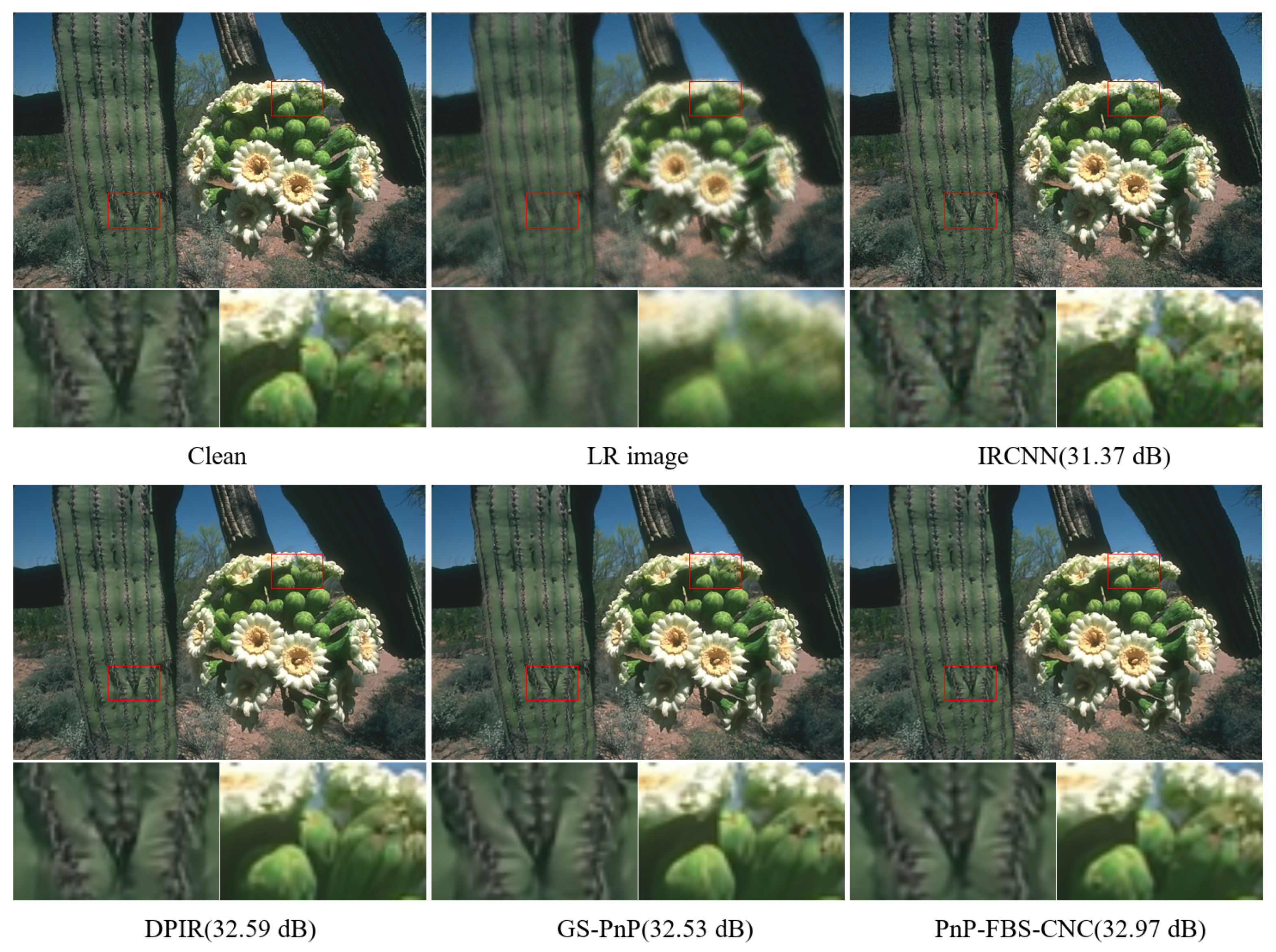
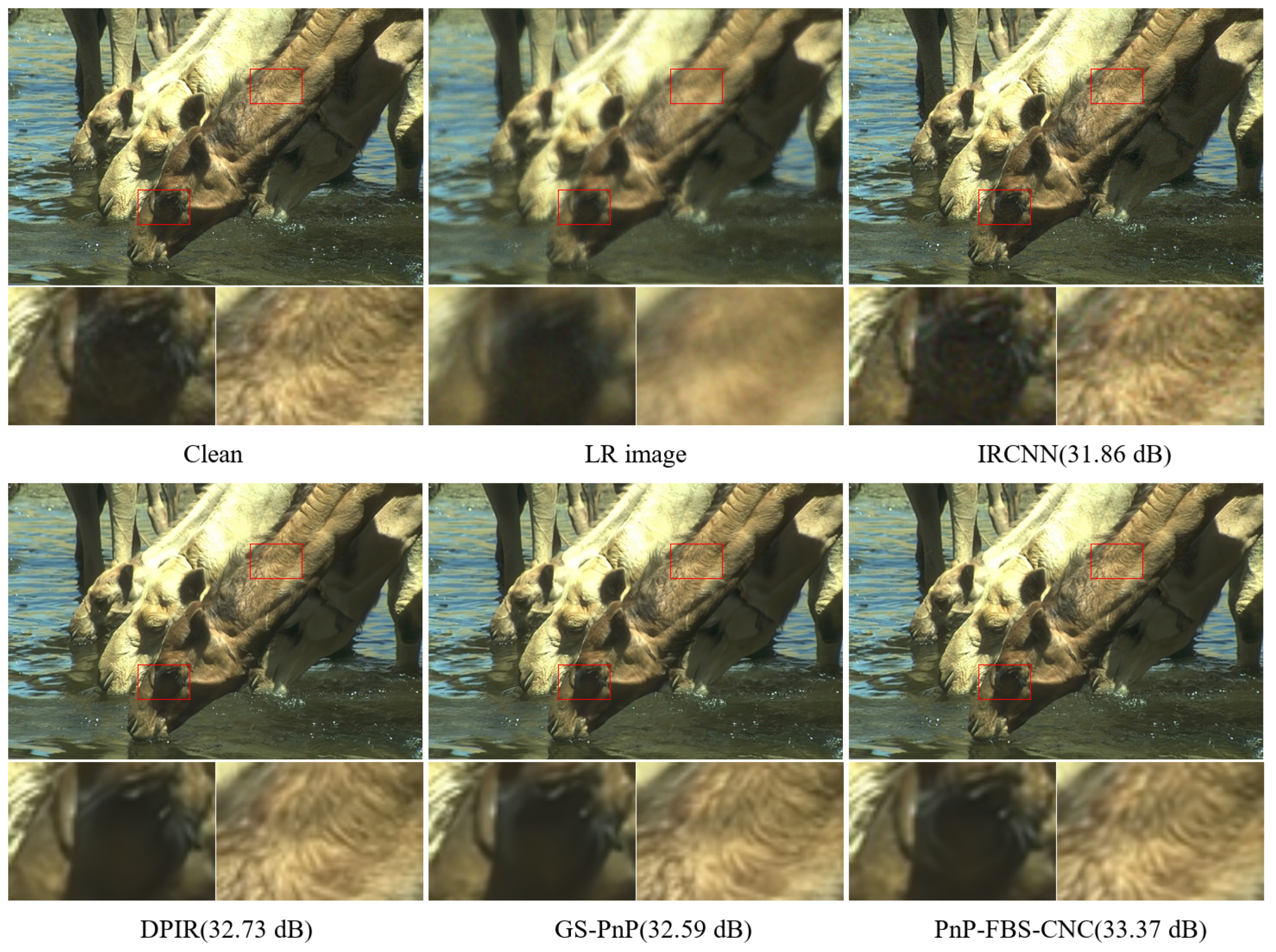
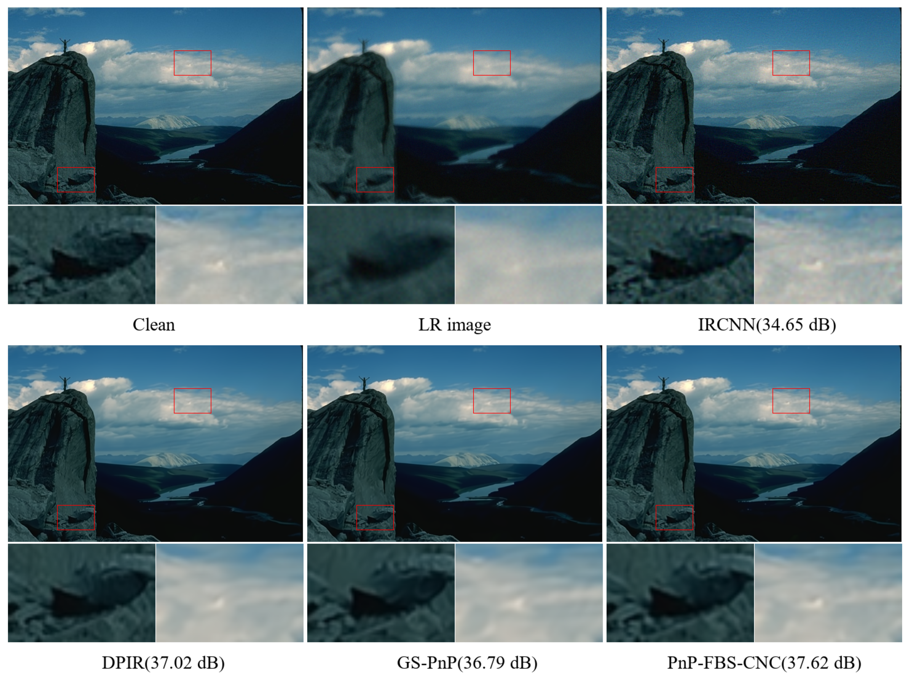
0.01	IRCNN	24.32	32.68	32.20	31.35	32.17	32.24	32.65	31.46	31.42
	DPIR	25.93	33.61	33.18	32.95	33.01	34.03	34.29	33.02	32.70
	GS-PnP	26.60	33.47	32.97	32.83	32.79	34.01	34.19	32.88	32.49
	PnP-FBS-CNC	24.28	33.98	33.56	33.37	33.45	34.48	34.69	33.38	33.16
0.03	IRCNN	27.58	29.25	28.81	28.84	28.56	29.72	29.61	28.82	28.49
	DPIR	28.15	29.31	28.98	29.13	28.68	30.14	30.17	29.25	28.82
	GS-PnP	30.57	29.16	28.82	29.13	28.54	30.26	30.15	29.26	28.86
	PnP-FBS-CNC	28.07	29.81	29. 49	29.68	29.25	30.67	30.66	29.77	29.37
0.05	IRCNN	30.24	26.92	26.67	27.16	26.29	28.22	28.00	27.14	26.75
	DPIR	31.52	27.45	27.26	27.67	26.91	28.55	28.27	27.71	27.23
	GS-PnP	32.67	27.38	27.21	27.63	26.92	28.63	28.36	27.74	27.33
	PnP-FBS-CNC	31.19	28.03	27.76	28.22	27.51	29.12	28.95	28.24	27.84

, effectively demonstrating the deblurring effects of the CBSD68 dataset with various blur kernels and noise levels. According to Table 1, it can be observed that the CPU time of PnP-FBS-CNC can be comparable with the other three algorithms. Moreover, PnP-FBS-CNC exhibits the highest average PSNR value irrespective of the chosen noise level and blur kernel. Simultaneously, we observe that when the noise level is 0.01, all methods yield significantly higher average PSNR values compared to those obtained at the other two noise levels. This indicates a positive correlation between decreasing noise levels and increasing average PSNR values.

We next assess the deblurring performance of these methods in terms of visual aspects. As indicated in Table 1, the optimal PSNR numerical performance is achieved when the noise level is 0.01. Therefore, we select the images with this noise level to examine the deblurring visual effect. Additionally, considering the extensive number of images available, we selectively choose three groups of images as exemplars to observe their respective deblurring effects. Meanwhile, we select different blur kernels for each of these three groups of images: kernel 1 with size $19\times 19$, kernel 3 with size $15\times 15$, and kernel 5 with size $13\times 13$. The corresponding visual comparison results for each method are illustrated in Figure 2, Figure 3 and Figure 4. After examining these images, it can be concluded that the quality of the images produced by IRCNN is comparatively inferior to those obtained by other methods. This distinction can be readily observed by comparing the water region of each image in Figure 2 and the blue sky region of each image in Figure 3 and Figure 4. We observe that the PnP-FBS-CNC method yields an image that is more closely aligned with the clean image and exhibits superior clarity in processing fine textures. The PSNR value displayed in the image indicates that PnP-FBS-CNC outperforms other methods in terms of deblurring performance.

In conclusion, the above performance demonstrates the superiority of the proposed algorithm for image deblurring, thereby strongly validating its effectiveness.

6. Conclusions

In this paper, we present the PnP-FBS-CNC algorithm for image deblurring. The incorporation of the CNC sparse regularization term significantly enhances the deblurring effect. Meanwhile, the PnP algorithm showcases its superiority as a powerful framework for addressing the sparse optimization problem. Furthermore, these advantages of our proposed algorithm are visually confirmed through experimental results.

References

- Zhang, K.; Ren, W.; Luo, W.; Lai, W.S.; Stenger, B.; Yang, M.H.; Li, H. Deep image deblurring: A survey. Int. J. Comput. Vis. 2022, 130, 2103–2130. [Google Scholar] [CrossRef]
- Eboli, T.; Sun, J.; Ponce, J. End-to-end interpretable learning of non-blind image deblurring. In Proceedings of the Computer Vision—ECCV 2020: 16th European Conference, Glasgow, UK, 23–28 August 2020; Part XVII 16. Springer: Berlin/Heidelberg, Germany, 2020; pp. 314–331. [Google Scholar]
- Yan, Y.; Ren, W.; Guo, Y.; Wang, R.; Cao, X. Image deblurring via extreme channels prior. In Proceedings of the IEEE Conference on Computer Vision and Pattern Recognition, Honolulu, HI, USA, 21–26 July 2017; pp. 4003–4011. [Google Scholar]
- Vasu, S.; Maligireddy, V.R.; Rajagopalan, A. Non-blind deblurring: Handling kernel uncertainty with CNNs. In Proceedings of the IEEE Conference on Computer Vision and Pattern Recognition, Salt Lake City, UT, USA, 18–22 June 2018; pp. 3272–3281. [Google Scholar]
- Liu, Y.; Sheng, Z.; Shen, H.L. Guided Image Deblurring by Deep Multi-Modal Image Fusion. IEEE Access 2022, 10, 130708–130718. [Google Scholar] [CrossRef]
- Zhang, M.; Young, G.S.; Tie, Y.; Gu, X.; Xu, X. A new framework of designing iterative techniques for image deblurring. Pattern Recognit. 2022, 124, 108463. [Google Scholar] [CrossRef]
- Zhang, K.; Li, Y.; Zuo, W.; Zhang, L.; Van Gool, L.; Timofte, R. Plug-and-play image restoration with deep denoiser prior. IEEE Trans. Pattern Anal. Mach. Intell. 2021, 44, 6360–6376. [Google Scholar] [CrossRef]
- Gavaskar, R.G.; Athalye, C.D.; Chaudhury, K.N. On plug-and-play regularization using linear denoisers. IEEE Trans. Image Process. 2021, 30, 4802–4813. [Google Scholar] [CrossRef]
- Gupta, A.; Joshi, N.; Lawrence Zitnick, C.; Cohen, M.; Curless, B. Single image deblurring using motion density functions. In Proceedings of the Computer Vision—ECCV 2010: 11th European Conference on Computer Vision, Heraklion, Crete, Greece, 5–11 September 2010; Part I 11. Springer: Berlin/Heidelberg, Germany, 2010; pp. 171–184. [Google Scholar]
- Krishnan, D.; Tay, T.; Fergus, R. Blind deconvolution using a normalized sparsity measure. In Proceedings of the CVPR 2011, Providence, RI, USA, 20–25 June 2011; pp. 233–240. [Google Scholar]
- Xu, L.; Tao, X.; Jia, J. Inverse kernels for fast spatial deconvolution. In Proceedings of the Computer Vision—ECCV 2014: 13th European Conference, Zurich, Switzerland, 6–12 September 2014; Part V 13. Springer: Berlin/Heidelberg, Germany, 2014; pp. 33–48. [Google Scholar]
- Pan, J.; Sun, D.; Pfister, H.; Yang, M.H. Blind image deblurring using dark channel prior. In Proceedings of the IEEE Conference on Computer Vision and Pattern Recognition, Las Vegas, NV, USA, 27–30 June 2016; pp. 1628–1636. [Google Scholar]
- Hurault, S.; Leclaire, A.; Papadakis, N. Gradient Step Denoiser for convergent Plug-and-Play. In Proceedings of the International Conference on Learning Representations (ICLR’22), Virtual Event, 25–29 April 2022. [Google Scholar]
- Fermanian, R.; Pendu, M.L.; Guillemot, C. Learned gradient of a regularizer for plug-and-play gradient descent. arXiv 2022, arXiv:2204.13940. [Google Scholar]
- Xu, L.; Zheng, S.; Jia, J. Unnatural L0 Sparse Representation for Natural Image Deblurring. In Proceedings of the 2013 IEEE Conference on Computer Vision and Pattern Recognition, Portland, OR, USA, 23–28 June 2013; pp. 1107–1114. [Google Scholar]
- Pan, J.; Hu, Z.; Su, Z.; Yang, M.H. Deblurring Text Images via L0-Regularized Intensity and Gradient Prior. In Proceedings of the 2014 IEEE Conference on Computer Vision and Pattern Recognition (CVPR), Columbus, OH, USA, 23–28 June 2014; pp. 2901–2908. [Google Scholar]
- Levin, A.; Weiss, Y.; Durand, F.; Freeman, W.T. Understanding and evaluating blind deconvolution algorithms. In Proceedings of the 2009 IEEE Conference on Computer Vision and Pattern Recognition, Miami, FL, USA, 20–25 June 2009; pp. 1964–1971. [Google Scholar]
- Danielyan, A.; Katkovnik, V.; Egiazarian, K. BM3D frames and variational image deblurring. IEEE Trans. Image Process. 2011, 21, 1715–1728. [Google Scholar] [CrossRef]
- Ye, Z.; Ou, X.; Huang, J.; Chen, Y. Infrared Image Deblurring Based on Lp-Pseudo-Norm and High-Order Overlapping Group Sparsity Regularization. Algorithms 2022, 15, 327. [Google Scholar] [CrossRef]
- Selesnick, I. Sparse regularization via convex analysis. IEEE Trans. Signal Process. 2017, 65, 4481–4494. [Google Scholar] [CrossRef]
- Selesnick, I.; Lanza, A.; Morigi, S.; Sgallari, F. Non-convex total variation regularization for convex denoising of signals. J. Math. Imaging Vis. 2020, 62, 825–841. [Google Scholar] [CrossRef]
- Lanza, A.; Morigi, S.; Selesnick, I.W.; Sgallari, F. Convex Non-Convex Variational Models. In Handbook of Mathematical Models and Algorithms in Computer Vision and Imaging: Mathematical Imaging and Vision; Springer: Berlin/Heidelberg, Germany, 2022; pp. 1–57. [Google Scholar]
- Lanza, A.; Morigi, S.; Selesnick, I.W.; Sgallari, F. Sparsity-inducing nonconvex nonseparable regularization for convex image processing. SIAM J. Imaging Sci. 2019, 12, 1099–1134. [Google Scholar] [CrossRef]
- Teodoro, A.M.; Bioucas-Dias, J.M.; Figueiredo, M.A. Image restoration and reconstruction using variable splitting and class-adapted image priors. In Proceedings of the 2016 IEEE International Conference on Image Processing (ICIP), Phoenix, AZ, USA, 25–28 September 2016; pp. 3518–3522. [Google Scholar]
- Kupyn, O.; Budzan, V.; Mykhailych, M.; Mishkin, D.; Matas, J. Deblurgan: Blind motion deblurring using conditional adversarial networks. In Proceedings of the IEEE Conference on Computer Vision and Pattern Recognition, Salt Lake City, UT, USA, 18–22 June 2018; pp. 8183–8192. [Google Scholar]
- Li, Y.; Tofighi, M.; Monga, V.; Eldar, Y.C. An algorithm unrolling approach to deep image deblurring. In Proceedings of the ICASSP 2019—2019 IEEE International Conference on Acoustics, Speech and Signal Processing (ICASSP), Brighton, UK, 12–17 May 2019; pp. 7675–7679. [Google Scholar]
- Mittal, T.; Agrawal, P.; Pahwa, E.; Makwana, A. NFResNet: Multi-scale and U-shaped Networks for Deblurring. arXiv 2022, arXiv:2212.05909. [Google Scholar]
- Tao, X.; Gao, H.; Shen, X.; Wang, J.; Jia, J. Scale-recurrent network for deep image deblurring. In Proceedings of the IEEE Conference on Computer Vision and Pattern Recognition, Salt Lake City, UT, USA, 18–22 June 2018; pp. 8174–8182. [Google Scholar]
- Liang, C.H.; Chen, Y.A.; Liu, Y.C.; Hsu, W.H. Raw image deblurring. IEEE Trans. Multimed. 2020, 24, 61–72. [Google Scholar] [CrossRef]
- Zou, W.; Jiang, M.; Zhang, Y.; Chen, L.; Lu, Z.; Wu, Y. Sdwnet: A straight dilated network with wavelet transformation for image deblurring. In Proceedings of the IEEE/CVF International Conference on Computer Vision, Montreal, QC, Canada, 10–17 October 2021; pp. 1895–1904. [Google Scholar]
- Tomosada, H.; Kudo, T.; Fujisawa, T.; Ikehara, M. GAN-based image deblurring using DCT loss with customized datasets. IEEE Access 2021, 9, 135224–135233. [Google Scholar] [CrossRef]
- Chen, T.; Chen, X.; Chen, W.; Wang, Z.; Heaton, H.; Liu, J.; Yin, W. Learning to optimize: A primer and a benchmark. J. Mach. Learn. Res. 2022, 23, 8562–8620. [Google Scholar]
- Mukherjee, S.; Hauptmann, A.; Öktem, O.; Pereyra, M.; Schönlieb, C.B. Learned Reconstruction Methods with Convergence Guarantees: A survey of concepts and applications. IEEE Signal Process. Mag. 2023, 40, 164–182. [Google Scholar] [CrossRef]
- Shlezinger, N.; Whang, J.; Eldar, Y.C.; Dimakis, A.G. Model-Based Deep Learning. Proc. IEEE 2023, 111, 465–499. [Google Scholar] [CrossRef]
- Ryu, E.; Liu, J.; Wang, S.; Chen, X.; Wang, Z.; Yin, W. Plug-and-play methods provably converge with properly trained denoisers. In Proceedings of the International Conference on Machine Learning, Long Beach, CA, USA, 9–15 June 2019; pp. 5546–5557. [Google Scholar]
- Zhang, K.; Zuo, W.; Gu, S.; Zhang, L. Learning deep CNN denoiser prior for image restoration. In Proceedings of the IEEE Conference on Computer Vision and Pattern Recognition, Honolulu, HI, USA, 21–26 July 2017; pp. 3929–3938. [Google Scholar]
- Nair, P.; Chaudhury, K.N. On the Construction of Averaged Deep Denoisers for Image Regularization. arXiv 2022, arXiv:2207.07321. [Google Scholar]
- Kamilov, U.S.; Bouman, C.A.; Buzzard, G.T.; Wohlberg, B. Plug-and-play methods for integrating physical and learned models in computational imaging: Theory, algorithms, and applications. IEEE Signal Process. Mag. 2023, 40, 85–97. [Google Scholar] [CrossRef]
- Li, J.; Li, J.; Xie, Z.; Zou, J. Plug-and-play ADMM for MRI reconstruction with convex nonconvex sparse regularization. IEEE Access 2021, 9, 148315–148324. [Google Scholar] [CrossRef]
- Xu, Y.; Qu, M.; Liu, L.; Liu, G.; Zou, J. Plug-and-play algorithms for convex non-convex regularization: Convergence analysis and applications. Math. Methods Appl. Sci. 2023. [CrossRef]
- Rudin, L.I.; Osher, S.; Fatemi, E. Nonlinear total variation based noise removal algorithms. Phys. D Nonlinear Phenom. 1992, 60, 259–268. [Google Scholar] [CrossRef]
- Dabov, K.; Foi, A.; Katkovnik, V.; Egiazarian, K. Image denoising by sparse 3-D transform-domain collaborative filtering. IEEE Trans. Image Process. 2007, 16, 2080–2095. [Google Scholar] [CrossRef]
- Selesnick, I. Total variation denoising via the Moreau envelope. IEEE Signal Process. Lett. 2017, 24, 216–220. [Google Scholar] [CrossRef]
- Perelli, A.; Lexa, M.; Can, A.; Davies, M.E. Compressive computed tomography reconstruction through denoising approximate message passing. SIAM J. Imaging Sci. 2020, 13, 1860–1897. [Google Scholar] [CrossRef]
- Zhao, X.L.; Xu, W.H.; Jiang, T.X.; Wang, Y.; Ng, M.K. Deep plug-and-play prior for low-rank tensor completion. Neurocomputing 2020, 400, 137–149. [Google Scholar] [CrossRef]
- Liu, T.; Yin, Q.; Yang, J.; Wang, Y.; An, W. Combining Deep Denoiser and Low-rank Priors for Infrared Small Target Detection. Pattern Recognit. 2023, 135, 109184. [Google Scholar] [CrossRef]
- Martin, D.; Fowlkes, C.; Tal, D.; Malik, J. A Database of Human Segmented Natural Images and its Application to Evaluating Segmentation Algorithms and Measuring Ecological Statistics. In Proceedings of the 8th International Conference on Computer Vision, Vancouver, BC, Canada, 7–14 July 2001; Volume 2, pp. 416–423. [Google Scholar]