A Markov Chain Genetic Algorithm Approach for Non-Parametric Posterior Distribution Sampling of Regression Parameters

Abstract

This paper proposes a genetic algorithm-based Markov Chain approach that can be used for non-parametric estimation of regression coefficients and their statistical confidence bounds. The proposed approach can generate samples from an unknown probability density function if a formal functional form of its likelihood is known. The approach is tested in the non-parametric estimation of regression coefficients, where the least-square minimizing function is considered the maximum likelihood of a multivariate distribution. This approach has an advantage over traditional Markov Chain Monte Carlo methods because it is proven to converge and generate unbiased samples computationally efficiently.

1. Introduction

Let α(x) be some unknown continuous multivariate probability density function. Let x_i = [x_i1,…, x_in] be the ith iid sample generated from the distribution. Assume that m such samples are available; then, a maximum likelihood estimator $\widehat{\alpha }$ will maximize the following expression:

$$\widehat{\alpha }\left(x\right)={\prod }_{i=1}^m\widehat{\alpha }\left(x_i\right)$$

(1)

If X and Y are random variables generated from multivariate distribution (X,Y),

$${\sum }_{i=1}^m{\left[y_i-\widehat{\alpha }\left(x_i\right)\right]}^2$$

(2)

where the dimensionality of some response variable Y is one and an iid sample from the distribution is represented as (x₁, y₁),…, (x_m, y_m). Then, the least-square non-parametric estimator will minimize the following expression [1]:

In regression problems, the dependence of y on x is considered to be given by some regression function $\widehat{\alpha }$(x) belonging to some class of functions [2]. In this paper, assuming that some functional model form $\widehat{\alpha }$(x) = f(x; θ₁,…, θ_n) is known or a priori established, parameters θ₁,…, θ_n are computed by minimizing the least-square expression in Equation (2). When the true density α(x) lies in the parametric class of functions parameterized by the vector θ = [θ₁,…, θ_n], then, finding parameters by minimizing Equation (2), i.e., maximizing the likelihood, properties such as convergence, consistency, and lack of bias are satisfied [3]. However, when actual density does not lie in the class of parametric functions, there is an acute need for non-parametric estimation [4].

Methods in Bayesian statistics condition the problem of learning parameters (θ) on the dataset D, which is used to learn the parameters. These methods allow for the specification of priors on the parameters as p(θ) and require a formal specification of data likelihood function p(D|θ), which is conditioned on the parameters θ. The learning of parameters and confidence bounds on the parameters occurs using Monte Carlo Markov Chain (MCMC) methods to estimate posterior distribution p(θ|D) via the following Bayesian rule:

$$p\left(\theta |D\right)\propto p\left(D|\theta \right)\times p\left(\theta \right)$$

(3)

To reduce any bias in confidence bounds on the parameters, samples from the initial burn-in period are excluded from the computation of confidence bounds.

The method described in this paper does not require any knowledge of data likelihoods or user-defined priors. The “population”-based method directly generates posterior distribution samples $p\left(\theta |D\right)$ so that confidence bounds on parameters can be generated. There is no need to exclude any initial burn-in period samples. More specifically, a genetic algorithm (GA) approach is used to estimate the parameters and their confidence bounds. This method begins with a random sample (i.e., population) estimate $p^0\left(\theta |D\right)$ and iterates over certain GA generations k so that a steady-state distribution of the sample,$p^k\left(\theta |D\right)$, minimizing the average least-square error, is obtained. It is shown that from one iteration to the next, the GA forms a Markov Chain, whose transition matrix can be determined using a fitness measure of minimizing the sum of squared error expression (2). Once the population converges, the final population can be used to establish confidence bounds on the regression parameters. The transition matrix is shown to be irreducible and aperiodic, which guarantees both the uniqueness of the steady-state distribution and convergence to a steady-state, regardless of the initial random population $p^0\left(\theta |D\right)$.

The rest of the paper is organized as follows: In Section 2, preliminaries of the GA Markov Chain framework are described. In Section 3, the approach is applied to a dataset, and the results of the experiments are reported. Section 4 concludes the paper with a summary and directions for future work.

2. A Genetic Algorithm Markov Chain and Related Preliminaries

A GA Markov Chain framework for steady-state distribution convergence was proposed both for binary GAs [5] and floating-point (real values) GAs [6]. This paper uses and adapts the GA floating-point framework. While the proposed method is general enough to learn parameters for both non-linear and linear regression functions, the linear model is used in this section for ease of exposition. The search for regression parameters occurs on a cone (a cone is a non-empty set C∈°ⁿ with vertex 0, such that if θ ∈ C ⇒ λθ ∈ C, ∀ λ ≥ 0). The benefit of searching for solutions on a cone is that the search for regression parameters can be restricted over the symmetric fixed closed interval, with a center at zero. Let that fixed interval be θ∈[−1, 1], and the true linear regression equation is represented as follows:

$$y_j={\sum }_{i=1}^n{\beta }_i{x}_j+{\beta }_{n+1}$$

(4)

where j = {1,…, m} is the index representing individual examples in the dataset D, i = {1,…, n} is the number of independent variables, β_is are regression coefficients, and ${\beta }_{n+1}$ is the regression intercept. When θ∈[−1, 1], the equivalent regression equation can be written as follows:

$$y_j=\lambda \left({\sum }_{i=1}^n{\theta }_i{x}_j+{\theta }_{n+1}\right)$$

(5)

The variable λ is a predetermined positive constant. The issue of selecting an appropriate value for this constant is taken up later in this section. For the rest of the paper, the dimensionality of θ = [θ₁,…, θ_z]^T, where the last parameter z = n + 1, is the intercept for the linear regression. When the correct regression model is learned, then $\lambda {\theta }_i={\beta }_i,i=\left\{1,\dots ,z\right\}.$

The GA used for the solution procedure is a random floating-point (real attribute) population-based search procedure, represented as a matrix Q^g. The rows of the matrix are equal to the size of the population (Ω) and the number of columns in the matrix is equal to z. For the sake of illustration, the matrix Q^g is represented as follows:

$$Q^g=\left[\begin{array}{ccc}{\theta }_{11}& \dots \dots & {\theta }_{1z}\\ .& \dots \dots & .\\ {\theta }_{\mathsf{\Omega }1}& \dots \dots & {\theta }_{\mathsf{\Omega }z}\end{array}\right]$$

(6)

The superscript “g” represents the generation number for the population. Each row represents a regression model described by its row parameters. In GA terminology, each row (regression model) is called a population member. A population member’s fitness is computed using the dataset D, applying the regression model using row parameters and Equation (5), and computing a reciprocal function of the root-mean-square error of Equation (2) as the fitness value. This approach to computing the fitness value means that population members with higher fitness values have lower root-mean-square errors. Each population member is represented with the subscript s = {1,…, Ω}, and an individual population member is defined as θ_s = [θ_s1,…, θ_sz]^T. Any component of population vector θ_s is called a gene of the population member s. All genes for all population members take values between −1 and 1, i.e., θ_si∈[−1, 1]. Initially, when g = 0, the values of genes for all population members are randomly generated over this interval using a uniform distribution. Next, for each population member, using the dataset D, its fitness is computed. The population for the next generation, i.e., g = 1, is computed by applying selection, crossover, and mutation operations. All of these three operations are probabilistic. The selection operator used in this research is proportional selection. The proportional selection operation selects two parents with replacement (i.e., two population members from Q⁰), wherein higher-fitness population members are more likely to be chosen as parents. Once these two parents are selected, a random crossover point is selected χ∈[1, z − 1], and then, with a certain crossover probability p_c, a child is created by exchanging the parents’ genes at crossover point χ. As an example, assume a crossover point χ∈[1, n − 1] and two selected parents, P_a = [θ_a1,…, θ_az] and P_b = [θ_b1,…, θ_bz], with a,b∈[1, Ω]; then, the genes of the child are created by swapping genes of parents at the crossover point, which will be $\left[{\theta }_{a1},\dots ,{\theta }_{a\chi },{\theta }_{b\left(\chi +1\right)},\dots ,{\theta }_{bz}\right]$. The mutation operation probabilistically changes a gene of a population member using a low mutation probability p_m. If a gene is selected for mutation, its value is replaced by generating a random number using uniform distribution in a closed interval [−1, 1]. If T^s, T^c, and T^m are represented as selection, crossover, and mutation operations, then the next generation population Q^g+1 is generated from the current generation population Q^g, as follows:

$$Q^{g+1}=T^m\left(T^C\left(T^S\left(Q^g\right)\right)\right)$$

(7)

The matrix Q^g in Equation (6) may be written as $Q^g={\left[{\theta }_1^T,\dots ,{\theta }_{\mathsf{\Omega }}^T\right]}^T$ and it is used to represent one state in a discrete Markov Chain. Each generation “g” is a discrete event. Given that genes or individual components of θ_s take continuous values in the interval [−1, 1], the interval is discretized into discrete categories using a minimal interval width δ > 0. The discretized interval will contain categories in a set {−1, −1 + δ, −1 + 2δ, …, 0, …, 1 − δ, 1}. By choosing a value of δ so that zero is not eliminated from the set, there will be η = (2/δ) total categories in the interval. Pendharkar [5] showed that the number of unique states, U, of the population will be given by the following expression:

$$U=\left(\begin{array}{c}{\eta }^z+\Omega -1\\ \Omega \end{array}\right)$$

(8)

The state of any population at any generation “g” can be represented by a vector π^g of dimension U, taking values in the interval [0, 1] so that the sum of the components of the vector always sum to 1. As an example, π⁰ = [0, 0, 1, … 0]^T means that the initial random population in generation 0 is in the third state of all possible unique states U. Assuming that the initial state of the population is given by the state π⁰ and the steady-state distribution (after several generations) is given by π*, the expression in Equation (7) is a Markov Chain, and iterative operations in Equation (7) can be represented as follows:

$${\left[{\pi }^{\mathrm{*}}\right]}^T={\left[{\pi }^0\right]}^{\mathrm{T}}R$$

(9)

where R is the Markov Chain transition matrix of dimension U × U. Let r_pq be the individual elements of matrix R; then, as long as p_m ≠ 0, r_pq > 0, because each population state can be reached by any other population state since a mutation can randomly change any gene of any or all population members with a non-zero low probability. Also, r_pq ≠ 1, because p_m ≠ 1 and because there is always some uncertainty that the population from state p may not go to state q in the next step. Furthermore, since each r_pq > 0 and r_pq ≠ 1, R is a stochastic matrix with the magnitude of its maximum eigenvalue equal to one and its second-largest eigenvalue less than one. The Markov Chain is ergodic and irreducible, with a unique stationary distribution that can be reached with any initial random population. It is important to note that steady-state distribution is reached when the average value of the GA fitness function is maximized for the GA population, which in the case of regression is equivalent to minimizing the least-square error. Pendharkar [6] provided an upper bound of Euclidean distance between steady-state distribution π* and population distribution probability vector π^g for mutation rates (i.e., mutation probability) p_m∈(0, 1). This upper bound is as follows:

$$‖{\pi }^{\mathrm{*}}-{\pi }^g‖\le min{\left(\left(1-{\left(p_m\right)}^{\mathsf{\Omega }z}\right),\left(1-{\left(1-p_m\right)}^{\mathsf{\Omega }z}\right)\right)}^g<1$$

(10)

The reader may note that Equation (10) gives an upper bound independent of any discrete interval chosen by selecting a particular value of δ. Neither δ nor η play any role in the upper bound; the bound is independent of the discretization of the [−1, 1] interval and is also applicable for the continuous interval [−1, 1]. The drawback of the bound defined in Equation (10) is that it is a loose bound. Albeit loose, the bound suggests that the convergence to steady-state distribution is guaranteed and is slower for large population sizes and many independent variables. Faster convergence can be obtained by selecting p_m values closer to 0.5. In deriving the upper bound, Pendharkar [6] assumed that the crossover probability is non-zero as well. The theoretical expression in Equation (10) can certainly be used to compute the total number of generations needed to achieve a certain level of accuracy for $‖{\pi }^{*}-{\pi }^g‖$. In practice, since the bound from Equation (10) is a loose bound, steady-state distribution occurs much earlier than the theoretical number of generations to convergence computed using Equation (10) suggests. In this research, the total number of generations when a GA run is terminated is represented by the symbol $\vartheta$. For a fixed value of $\vartheta$, the worst-case computational complexity of the GA procedure is O(${\mathsf{\Omega }}^2)$.

One of the benefits of the loose bound from Equation (10) is that it is independent of the crossover rate or type of crossover operations used in the GA. This means that different crossover operations can be used, and the mutation-driven loose bound from Equation (10) will still hold for these different crossover operations. As a result, this research uses two crossover operations. The first crossover operation is the single-point crossover operation described earlier. The second crossover operation is the arithmetic crossover [7]. 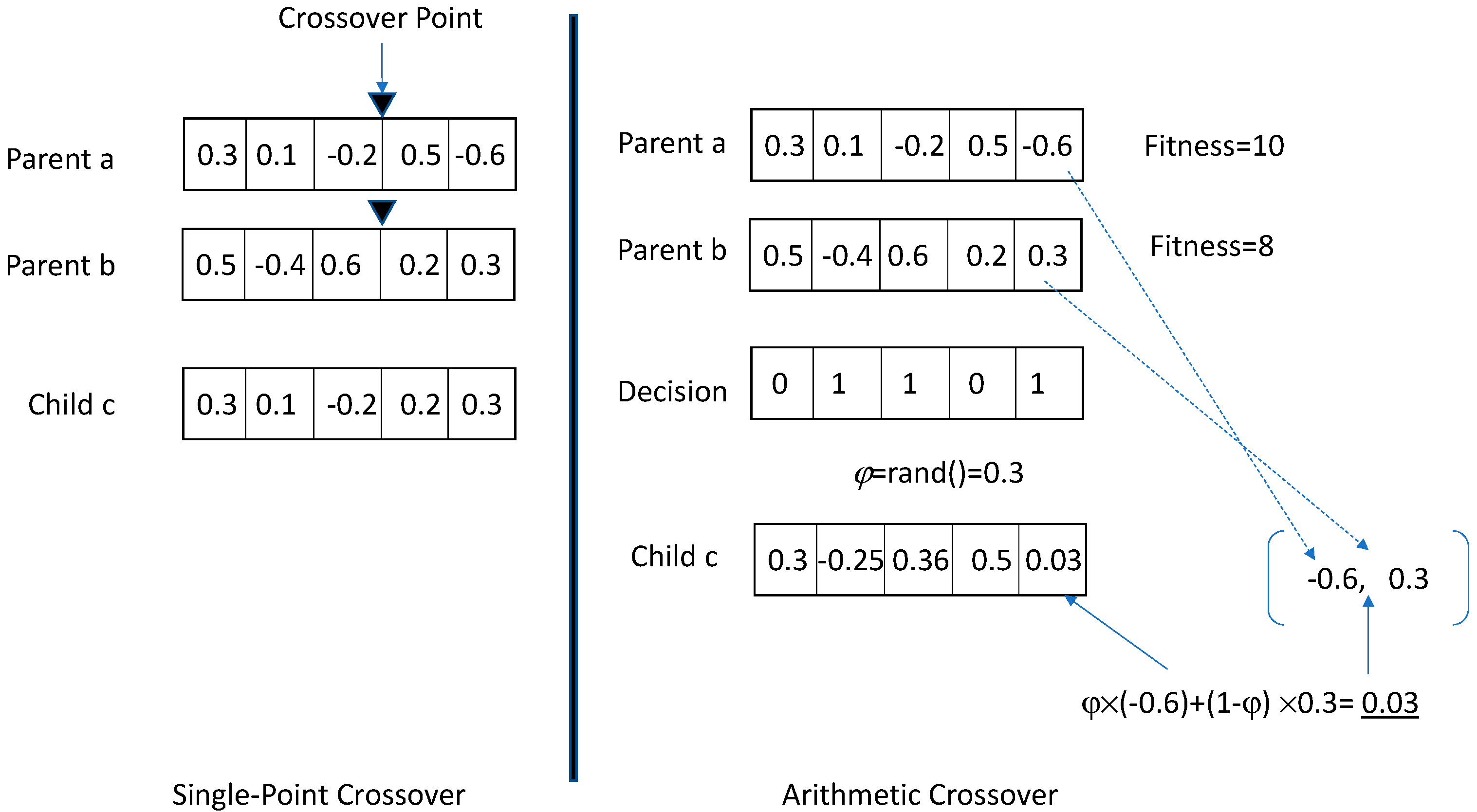Figure 1 illustrates the two crossover operations used in this research. As explained before, the single-point crossover picks two parents, a random crossover point, and it creates a child with genes containing the genes from the head of the first parent until the crossover point and genes from the tail of the second parent after the crossover point. The critical point to notice in this crossover is that the child’s genes take values from those appearing in two parents. The arithmetic crossover selects two parents using the selection operation and then considers the fitness values of the two parents. The higher-fitness parent becomes the base parent, whose genes will be retained unless the decision vector suggests a decision to change its genes. The decision vector, with a dimensionality equal to the number of genes, is a binary vector that selects a value of 0 or 1 with equal probability. For genes where the decision vector takes a value of 0, the higher-fitness parent’s genes are retained in the child. For genes where the decision vector takes a value of 1, the child’s gene (θ_ci) is replaced by a computed value, which is a weighted average of the respective genes of the two parents. The weights in this weighted average are assigned by generating a random number φ∈(0, 1) and averaging respective genes from the parents using the following formula:

$${\theta }_{ci}={\theta }_{ai}\times \phi +\left[\left(1-\phi \right)\times {\theta }_{bi}\right].$$

(11)

In Equation (11), the higher-fitness base parent is assumed to be the parent “a” with genes P_a = [θ_a1,…, θ_az]. There are some advantages of arithmetic crossover. First, arithmetic crossover produces gene values in the child that are weighted averages of the corresponding gene values of the parents. Second, these values are not random but are generated within the upper bounds of the respective gene values of both parents. Additionally, there are no biases in the arithmetic crossover, as all genes have an equal probability of crossover, and the weighted average improves the precision of parameters when parents have somewhat similar genes. As an example of bias, the first gene of parent a and the last gene of parent b will always be present in child c when a single-point crossover is used because the crossover point will always include the first gene and retain the last gene in the child. This situation is eliminated in arithmetic crossover, since the decision vector may contain one in the first and last gene locations.

Let Q* be the population at a generation where steady-state distribution is achieved with a desired level of accuracy. The steady-state population Q* is a sample generated from an unknown non-parametric distribution whose likelihood function is maximized using the GA’s minimizing least-square error fitness function. Using Q* as a sample for posterior distribution, the sample with regression parameters shown in Equation (4) can be obtained by multiplying matrix Q* by a scalar λ. Once the resulting matrix is obtained, non-parametric distribution confidence intervals for regression parameters can be established.

Earlier, it was assumed that the value of scalar λ was known and was assumed to be a constant. There are two ways to determine the value of λ. In the first sequential search approach, an initial value of λ = 10 is selected, GA experiments are run, and the population member with the best fitness is found. Using the genes of this population member, the value of λ, and Equation (5), the regression function in Equation (4) is estimated, and its root-mean-square (RMS) error on the dataset is computed and stored for comparison. Next, the value of λ is incremented by 1 to the next value, and the procedure is repeated for a new value of λ and a new value of RMS is computed. If the RMS for the current value (i.e., λ = 11) is better than the previously stored RMS value (i.e., λ = 10), then the current value of RMS is stored for comparison and λ is incremented by 1 to the next value (i.e., λ = 12), and a similar procedure is repeated. Otherwise, the previous value of λ is selected as the final value of λ. The second approach is a direct approach that benchmarks the value of λ by using the results from traditional parametric statistical regression function parameters. Let these parameters from the traditional parametric statistical regression function be represented as a vector ${\left[{\beta }_1^{’},\dots ,{\beta }_{n+1}^{’}\right]}^{\mathrm{T}}$; then, the value of λ is computed using the following expression:

$$\lambda =max\left(\left|{\beta }_1^{\mathrm{’}}\right|,\dots ,\left|{\beta }_{n+1}^{\mathrm{’}}\right|\right)+1.$$

(12)

The second approach has one additional benefit that helps speed up the convergence of the GA procedure. Since the regression function parameters from traditional regression are available, the genes of some members of an initial random population can be seeded by considering the value of λ and adding minor random noise to the known traditional regression parameters. This seeding ensures that the initial GA population is no longer entirely random and has some solutions close to traditional regression parameters and near-unknown optimum solutions. Longer run times are sometimes necessary to achieve population convergence without a seeding. Given these added computational efficiency benefits, this research uses the second approach for determining the value of λ and partial seeding of an initial random population. The seeding procedure used in this research first creates a random initial population. Next, for Ω times, it randomly picks a population member with replacement, randomly selects one of its genes, and assigns it a value using the following expression:

$$\frac{{\beta }_i^{\mathrm{’}}}{\lambda }\times rand\left(\mathrm{0,1}\right),$$

(13)

where rand(0,1) is a randomly generated number, taking its value between 0 and 1, and i is the index of the selected gene. Once this procedure is complete, the initial population becomes the seeded initial population. The reader may note that some members of the seeded initial population will contain all random genes because selecting the population member for seeding is a bootstrap sampling procedure. Furthermore, only one gene of a chosen population member is seeded, and that too has some random noise inserted in it, as shown in Equation (13). Seeding procedures are also used in MCMC and are sometimes called better starting points. The seeding procedure used here is somewhat weaker than those used in MCMC algorithms, where starting values for all parameters are seeded using values closer to the mode of the posterior distribution to improve convergence [8].

Using the final generation of the population at convergence, the central tendency parameters (means and medians) and probability intervals for regression parameters can be computed by first computing the means and probability intervals of θ_is for i = {1,…, n + 1} and then multiplying these values by the parameter λ obtained from Equation (12). The mean values for the θ_is are column averages for the final population from the matrix shown in Equation (6). In the final population at convergence, each column represents a sample from the posterior distribution of a regression function parameter. A 100 × (1 − γ)% confidence interval can be estimated by taking 100 × (γ/2)% and 100 × (1 − γ/2)% quantiles of the parameter sample, representing end points of the interval.

Once the value of λ is known and the statistical significance level for the confidence interval, γ, is decided, the initial no-information interval width (IW) can be determined. For example, if γ = 5%, the initial no-information IWs for parameters in Equation (4) are [−0.975 × λ, 0.975 × λ]. For the GA procedure, to add value, the final parameter IWs should be smaller than the initial no-information IWs. A formal method for computing the reduction in the final GA procedure IWs from the initial no-information IWs is mentioned in the next section.

3. Experiments and Results

The regression data selected for the experiments are related to the quality of the delivery system network of a soft drink company [9]. The dependent variable in the data is the time needed by an employee to restack an automatic soft drink vending machine. This time is called the total service time and is measured in minutes. There are two independent variables: the first variable is the number of stocked items, and the second is the distance an employee walks, measured in feet. The dataset contains 25 observations.

Table 1. Soft drink restacking times dataset.

Observation	Total Items	Total Distance	Total Time
1	7	560	16.68
2	3	220	11.5
3	3	340	12.03
4	4	80	14.88
5	6	150	13.75
6	7	330	18.11
7	2	110	8
8	7	210	17.83
9	30	1460	79.24
10	5	605	21.5
11	16	688	40.33
12	10	215	21
13	4	255	13.50
14	6	462	19.75
15	9	448	24
16	10	776	29
17	6	200	15.35
18	7	132	19
19	3	36	9.5
20	17	770	35.1
21	10	140	17.9
22	26	810	52.32
23	9	450	18.75
24	8	635	19.83
25	4	150	10.75

illustrates this dataset.

When the ordinary least-square (OLS) regression is run on the dataset, it results in parameter values of ${\beta }_1^{’}$ = 1.61591, ${\beta }_2^{’}$ = 0.0143848, and ${\beta }_3^{’}$ = 2.34123. The overall regression model is significant at a 95% statistical confidence level, and the adjusted R-squared value is 95.4%. The root-mean-squared (RMS) error for the OLS model is 3.05766. From Equation (12), the λ value is 3.34123. The no-information IW for non-parametric posterior distribution regression parameters β₁, β₂, and β₃ is [−3.2577, 3.2577] for a value of γ = 5%.

Some implementation aspects of the procedure were not described in Section 2. First is the fitness function of the GA procedure. For a given population member, the predicted outputs are computed from its genes using Equation (5). The RMS error on the dataset is computed next. Let us say that this RMS error is ξ_s for some population member model s∈{1,…, Ω}. The fitness value for this population member s in generation g, ($f_s^g$), is computed using the following expression:

$$f_s^g=\frac{\lambda }{1+{\xi }_s}$$

(14)

The maximization of Equation (14) can be obtained by minimizing the RMS. Note that λ is a predetermined constant. The number “one” in the denominator is added to avoid dividing by zero if ξ_s takes a value of zero in the event of a perfect regression model fit. Using the results of the OLS and plugging them into Equation (14), we obtain a value of 0.823. This value gives a benchmark of what may be the approximate best value of the best-fitness member in the GA procedure. If the best member fitness function value exceeds 0.823, then the GA model procedure has found a regression model with a lower RMS than the OLS regression model. Usually, it would be rare to find better results from a heuristic GA regression model. Thus, the threshold value of 0.823 should be considered an upper bound on the fitness value of the best population fitness member found using the GA experiments. Second, the no-information IW for the regression parameters was computed as [−0.975 × λ, 0.975 × λ] for the value of γ = 5%. If for the GA population considered for computing the final posterior distribution sample, the lb = 100 × (γ/2)% and ub = 100 × (1 − γ/2)% quantiles represent lower and upper bounds for a given regression parameter, then the percentage improvement in parameter IW from the no-information IW can be computed using the following expression:

$$PercentageIWImprovement(\mathrm{\%}imp.)=\left(1-\frac{\left(ub-lb\right)}{2\times \left(1-\gamma \right)\times \lambda }\right).$$

(15)

Finally, in Section 2, it was mentioned that a posterior distribution sample from the final population at convergence is considered for the computing parameter confidence intervals. Since the mutation operation introduces some randomness, it is not always necessary to pick the last generation of the population to compute a parameter confidence interval. From a practical standpoint, a sample is extracted from generation g* for population Q*, where g* is determined using the following expression:

$$g^{\mathrm{*}}=\underset{g\in \{0,\dots \vartheta \}}{\mathrm{argmax}}\left(\frac{\sum _{s=1}^{\mathsf{\Omega }}{f}_s^g}{\mathsf{\Omega }}\right)$$

(16)

Equation (16) implies that a sample is extracted when the average population fitness value is highest. Generally, this extraction generation is closer to the final population generation $\vartheta$, but it may or may not be the final population at generation $\vartheta$.

The objective of using a GA for learning regression parameters is like running a ridge regression to avoid overfitting the training dataset. As a heuristic procedure, in most cases, a GA-based regression model may not outperform OLS in terms of the RMS error. Still, it may provide better generalizability for unseen future cases, leading to improved predictability compared to the traditional OLS regression model. Given a small dataset, three regression parameters, and an initial seeded population, minor initial experiments were conducted to select GA parameters for the experiments. These parameters were Ω = 100, $\vartheta =200$, p_c = 30%, and p_m = 5%. The reader should note that the initial population in the procedure used in this research was always random for each run. This randomization was obtained using a random number that uses computer clock times as a seed for generating a random number. There are random number generators that allow users to define the seed for the random number generation procedure. When such a random number generator is used, the same initial population can be generated for each run by keeping the value of the seed constant. In such cases, the selection of parameters will be essential because then the parameters are the only criteria that will govern the quality of the final results. However, when the initial population for each run is randomly generated using computer clock times, the impact of parameters on the quality of solutions is hard to ascertain. In the case of computer clock time-seeded random numbers for the same set of parameters, slightly different results can be obtained owing to different starting populations. Extensive experiments on GA parameters in such a case are not necessary. Different runs with different initial populations can be conducted, and the percentage improvement criterion highlighted in Equation (15) can be used to separate high-quality results from low-quality results. Additionally, the average fitness of the GA population can be compared with the benchmark mentioned earlier (a value of 0.823) to monitor the gap between the average population fitness and its upper bound value, with a lower gap representing a better solution. The GA literature advises against using very high mutation rate values because high mutation rates introduce randomness [10]. Some randomness is necessary for searching for better solutions, but too much randomness can be detrimental to solution quality [10]. A general rule of thumb is that the crossover rate value should be less than 50%, and the mutation rate value should be less than the crossover rate value. Additionally, both the crossover rate and mutation rate should be non-zero values. In this paper, multiple runs were conducted with different starting populations and only the best results are reported.

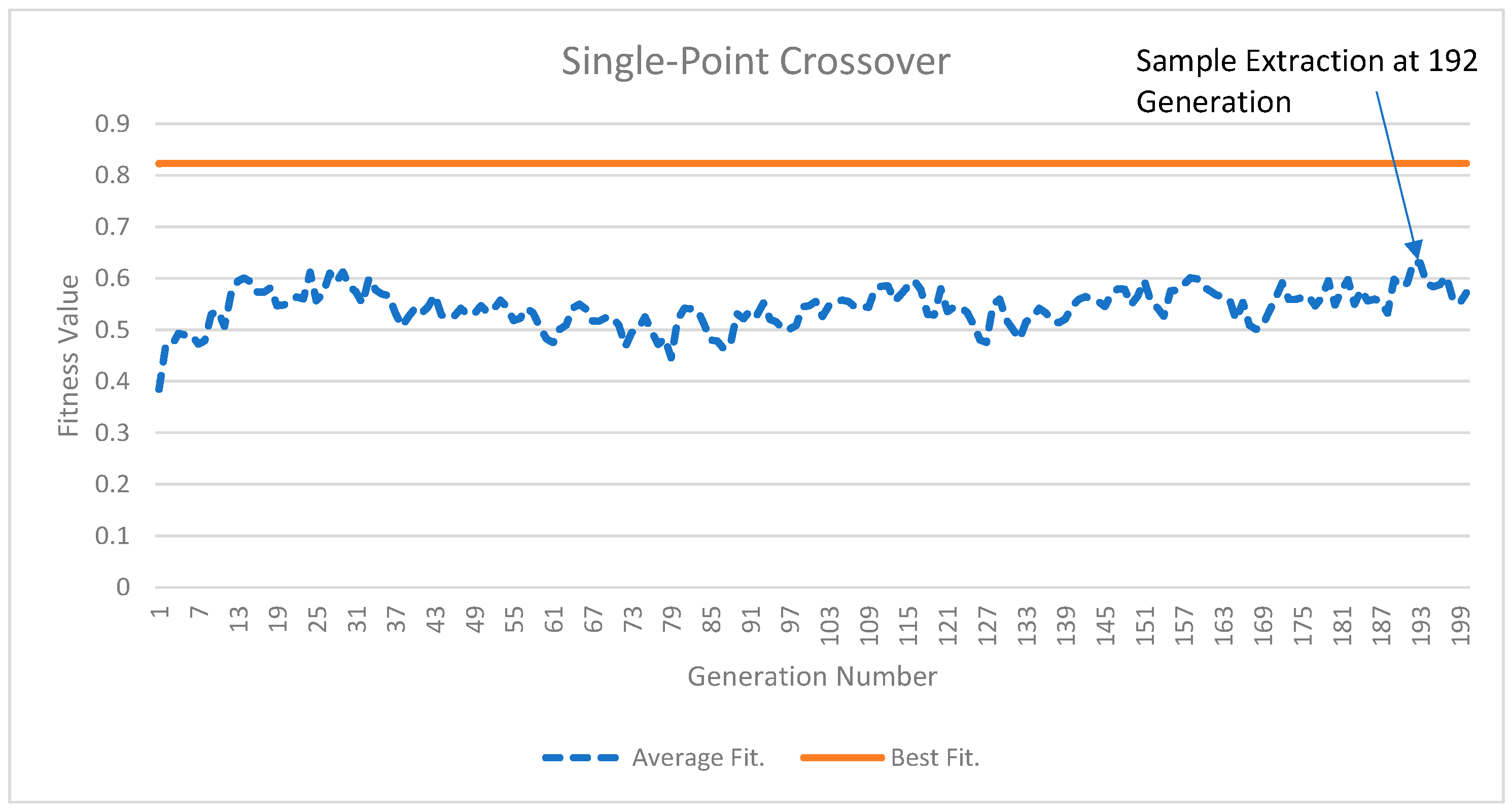
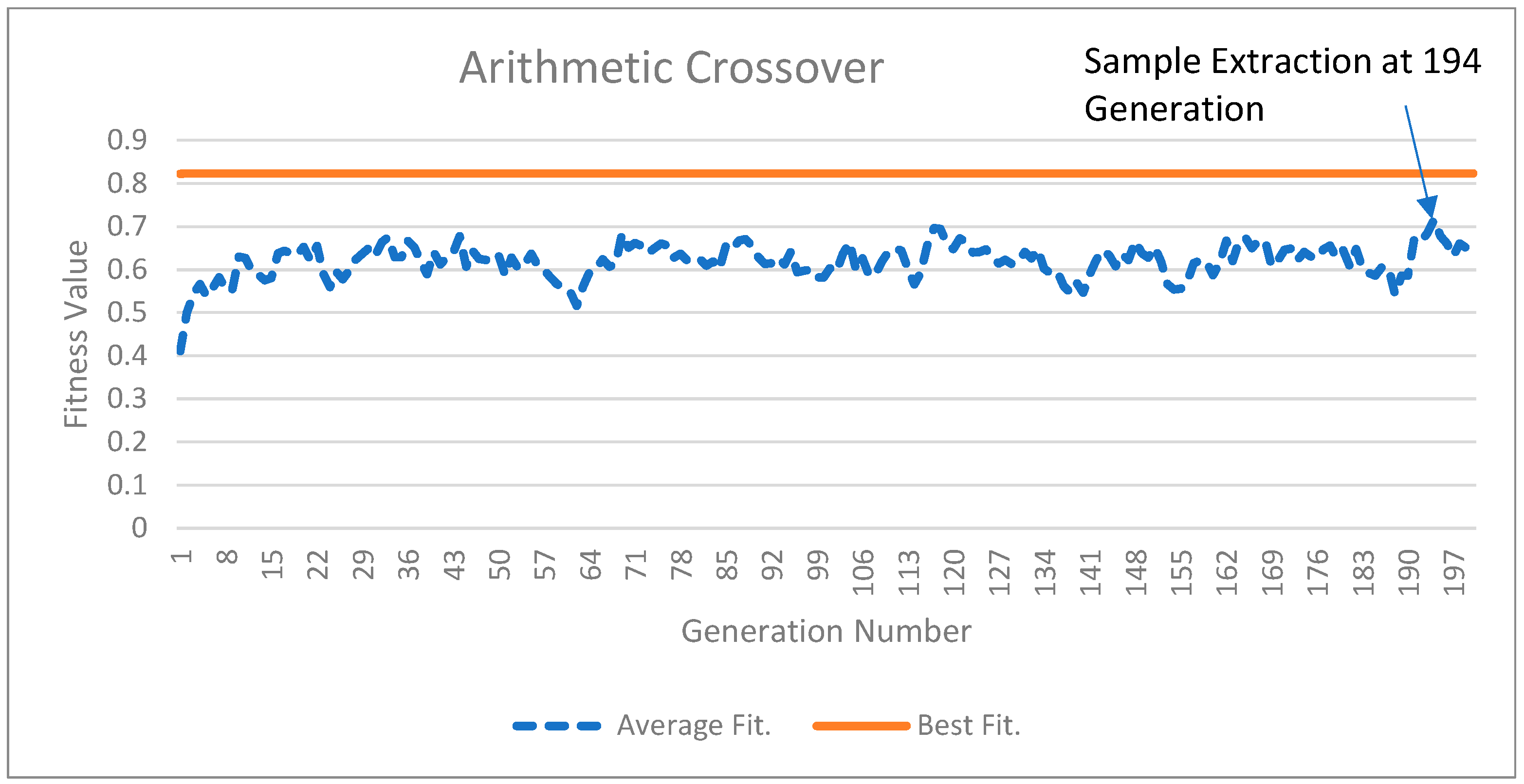
Figure 2 and Figure 3 illustrate the results of the GA experiments for two crossover operations. In both Figure 2 and Figure 3, the top solid line is the best-fitness population member and the dotted line is the average population members’ fitness. While the top line appears straight, minor improvements in the best population member fitness occur. For Figure 2, the best population member fitness value improves from 0.823015 in the 1st generation to 0.823325 in the 200th generation. In Figure 3, these numbers are 0.822516 and 0.823437, respectively. The average fitness values for the posterior distribution sample extracted at the 192nd generation from Figure 2 and the 194th generation for Figure 3 were 0.631558 and 0.714597, respectively. The higher average fitness value for the sample extracted from Figure 3 suggests that arithmetic crossover results are better and will provide a greater percentage of IW improvement (PIWI) from Equation (15). The reader may also visually observe the gap between the average population fitness values and the best fitness population member values. This gap is lower in Figure 3, indicating that arithmetic crossover results are better than single-point crossover results.

Table 2. Posterior distribution summaries.

Parameter	Mean	Std. Dev.	2.5%	Median	97.5%	PIWI
Single-Point Crossover Results
β1	1.548	0.66	−0.702	1.712	1.712	61.98%
β2	0.073	0.64	−0.635	0.015	2.279	54.10%
β3	0.984	1.18	−2.907	1.069	2.416	16.16%
Arithmetic Crossover Results
β1	1.491	0.71	0.568	1.604	1.604	83.68%
β2	0.003	0.62	−1.203	0.015	1.450	58.21%
β3	2.089	0.93	−1.036	2.331	2.331	46.97%
Bayesian Model Results (Taken from [9])
β1	1.610	0.18	1.272	1.609	1.968
β2	0.014	0.01	0.007	0.014	0.022
β3	2.356	1.19	−0.039	2.372	4.635

illustrates the descriptive statistics of results obtained from the two crossover operators. Bayesian regression results taken from a text [9] are also reported for comparison. As expected, the PIWIs are higher for the arithmetic crossover, with all PIWIs being higher than 46%. This results in a tighter 95% confidence interval of the GA regression parameters for the arithmetic crossover operator. In all cases, the arithmetic crossover operator PIWIs are higher than those for the single-point crossover operator. A point of interest for the reader may be to note the starting average fitness values for both crossover operations at generation one. Both operators start at an average fitness value of around 0.4. Since the initial GA population is seeded with values close to the OLS regression parameters, the starting point illustrates that there is enough diversity in the population for the GA operators to still evolve the population to a higher overall fitness.

When viewing the arithmetic crossover results with the Bayesian model results, the Bayesian model confidence bounds are tighter, partly due to the likelihood distribution assumptions that Bayesian models make. The only exception is the confidence bound for the regression intercept, which is lower for the GA regression model. The non-parametric distribution is negatively skewed since the mean values for arithmetic crossover GA models are always lower than the median values. When tight bounds are desired, it is possible to use the GA regression model first to understand the underlying properties of the non-parametric posterior distribution and then select the appropriate data likelihood and prior distributions in Bayesian regression. This way, Bayesian regression modelers can make an informed decision and improve confidence in the results of their investigations.

Table 3. The best member fitness function parameters.

GA Model	β1	β2	β3	RMS
Single-Point Crossover	1.605	0.014	2.416	3.058
Arithmetic Crossover	1.616	0.014	2.331	3.057

illustrates the parameter values for the best-fitness population member found in all GA generations. Both models provide somewhat similar results in terms of RMS values, which in turn are identical to the RMS results obtained through OLS regression. Given that there are three values for a regression parameter (mean, median, and best-fitness population member genes), the question is, which value should be used as the final set of regression parameters? A decision maker should use the best member fitness parameter values from Table 3 if those values fall within the 95% confidence bounds provided in Table 2. For arithmetic crossover, the value for β₁ = 1.616 does not belong to its 95% confidence bounds of [0.568, 1.604] from Table 2. Thus, it should be rejected. The reason for this rejection is that the value of β₁ = 1.616 may not be a natural outcome of GA population evolution but was retained due to the initial seeding of the GA population with OLS regression parameters. Once a value for the best member fitness is rejected, the median values should be used as the final set of regression parameters. Ideally, the best fitness values should be chosen if these values fall within their respective 95% confidence bounds. Otherwise, median values represent the next best solution. In the case of single-point crossover, the best member fitness values fall within the 95% confidence bounds provided in Table 2, which are the final set of regression parameters.

It may be possible to use an ensemble value, the average of all three values (median, mean, and best member fitness genes) as the final value for the regression model. The merits of different approaches in deciding the final set of regression function parameters are considered to be out of scope for the current study. However, multiple values offer different selection possibilities, where each possibility may have advantages and disadvantages.

4. Summary and Directions for Future Research

This paper proposes a GA-based Markov chain approach to directly generate samples from posterior distributions. Using linear regression as an example and least-square error minimization criteria, a sample from posterior distribution was extracted, and 95% confidence bounds on the regression parameters were established. This procedure is guaranteed to converge as long as non-zero parameter values for the GA are selected. Compared to traditional MCMC methods, the proposed method has certain advantages in that the procedure searches for all parameters simultaneously instead of one parameter at a time, as in MCMC methods. Also, no proposal density functions are required, and no burn-in period sample rejection is necessary. Knowledge of data likelihood and priors is not required as well. It is well known that MCMC methods do not allow for incorporation of multi-mode distribution [11] and the current method does not impose such restrictions either. The only challenge in using this method is that some knowledge of the maximum likelihood criterion for the posterior distribution is necessary. This knowledge is directly used for creating the GA fitness function.

There are some areas that could be explored where the proposed approach may be helpful. One of the advantages of the proposed method is that it does not require a continuous or differentiable likelihood function. The method may be adapted to generate truncated posterior distributions by imposing penalties in the GA fitness function. These penalties may be imposed by using IF–THEN rules. As noted earlier, the proposed method can also be used to aid in selecting data likelihood density functions for MCMC methods. While the linear regression problem domain was used in this research due to its widespread application and simplicity, the proposed method can easily be used for non-linear regression and linear and non-linear discriminant analysis. This method is likely more efficient than MCMC methods and will likely converge faster. When both the current method and the MCMC method can be used on a problem domain (as was the case in this research), both can be used to gain confidence in the final results. When results vary, it is possible to use the data-mining literature to devise approaches to combine different values to reduce error variance and gain confidence in the selected set of parameters. Future research is needed to explore the additional merits of the proposed GA procedure.