Generator of Fuzzy Implications

Abstract

In this research paper, a generator of fuzzy methods based on theorems and axioms of fuzzy logic is derived, analyzed and applied. The family presented generates fuzzy implications according to the value of a selected parameter. The obtained fuzzy implications should satisfy a number of axioms, and the conditions of satisfying the maximum number of axioms are denoted. New theorems are stated and proven based on the rule that the fuzzy function of fuzzy implication, which is strong, leads to fuzzy negation. In this work, the data taken were fuzzified for the application of the new formulae. The fuzzification of the data was undertaken using four kinds of membership degree functions. The new fuzzy functions were compared based on the results obtained after a number of repetitions. The new proposed methodology presents a new family of fuzzy implications, and also an algorithm is shown that produces fuzzy implications so as to be able to select the optimal method of the generator according to the value of a free parameter.

1. Introduction

The degree of truth of a proposition is expressed by fuzzy logic. Classical logic theory for 2500 years (Aristotelian logic) dealt with values 0 (false) or 1 (true). The two-valued classical logic was followed by the new theory of fuzzy logic, which brought about a revolution stating that apart from the values 0 and 1, there is an infinite number of values in the interval [0, 1] that express the value of a proposal. Fuzzy logic seeks the truth of propositions, and their degree of truth [1]. Thus, in fuzzy logic authors do not only encounter the concepts of cold and hot, but also intermediate states such as lukewarm or moderately hot, with various temperatures. Fuzzy logic creates verbal variables such as very good, good, average and bad, with each category constituting a fuzzy set. It is obvious that fuzziness contains special knowledge that is required in the assessment of a situation. People perceive the world better when using shades of gray in contrast to black (1) and white (0). Fuzzy logic operates in an environment of ambiguity and uncertainty to produce results that make sense to humans. Today, the theory of fuzziness finds huge applicability in the sectors of computing and artificial intelligence.

In this paper, the authors proposed a new type of fuzzy implications using a set of axioms and operations of fuzzy logic (fuzzy negations, probor and t-conorm). In order to apply the new family of fuzzy implications created, the authors used temperature and humidity data. For the fuzzification of all temperature and humidity values, four membership degree functions were constructed. The calculation of membership degrees of 122 temperature and humidity values using two triangular membership degree functions and two trapezoidal membership functions (isosceles and scalene triangular, isosceles and random trapezium) is based on a new type of calculation of fuzzy implication. After these stages, the authors performed extensive tests to find the value of m of fuzzy implication, so that the above formula can derive a value greater than or equal to 0.9, and the optimal value equal to 1.

The aim of this research was to obtain the number of repetitions needed such that the new fuzzy implication will take the optimal value 1 or a value greater than 0.9 in each membership degree function (isosceles trapezium, random trapezium, isosceles triangle, scalene triangle). Also, the basic purpose of this paper was to calculate, for each membership degree function, the precise number of temperature and humidity pairs, wherein the fuzzy implication has taken the chosen values.

The theoretical contribution of this work is that the authors used many axioms and theorems of fuzzy logic (fuzzy negations, t-conorm) so as to create a new and innovative type of fuzzy implication using the binomial Newton. This type of fuzzy implication represents a new family of fuzzy implications presented for the first time as part of fuzzy logic.

1.1. Literature Review-Related Work

Fuzzy implications are useful in a wide range of applications. In the literature, there are many families and classes of fuzzy implications that have been obtained from binary operations on the unit interval [0, 1], i.e., from basic fuzzy logic connectives, such as t-norms, t-conorms and negations. Moreover, investigations into complex fuzzy logic operators have focused on conjunction, disjunction and negation operators.

Makariadis et al. [2] presented the form of an implication using fuzzy negations constructed with the help of conic sections. The relation was applied to real temperature and humidity data of E.M.Y with full applications. Pagouropoulos et al. [3] presented a method for detecting the most suitable fuzzy implication among others under consideration, which incorporates an algorithm for the separation of two extreme cases. According to the truth values of the corresponding fuzzy propositions, the optimal implication is one of these two extremes. Pagouropoulos et al. [4] constructed a method for detecting the most suitable fuzzy implication among others under consideration by evaluating the metric distance between each implication and the ideal implication for a given data application. The ideal implication I is defined and used as a reference in order to measure the suitability of fuzzy implications. The method incorporates an algorithm that results in two extreme cases of fuzzy implications regarding their suitability for inference making; Botzoris et al. [5] proposed a method of evaluation of the different fuzzy implications using available statistical data. The choice of the appropriate implication is based on the deviation of the truth value of the fuzzy implication from the real values, as described by the statistical data. Rapti and Papadopoulos [6] introduced a new construction method of a fuzzy implication from n increasing functions g_i: [0, 1] → [0, ∞), (g(0) = 0) (i = 1, 2, :::, n, n ∈ N) and n + 1 fuzzy negations N_i (i = 1, 2, :::, n + 1, n ∈ N). This method allows authors to use at least two fuzzy negations Ni and one increasing function g in order to generate a new fuzzy implication. Bedregal et al. [7] showed a method of S-implication using two S-implications. The resulting implication S is satisfactory. The new implication is applied to the soundness property and some properties of the known S-implication. Balasubramaniam [8] investigated the conditions under which natural negation is transformed so that implication becomes equal to strong negation. Sufficient conditions are also presented for fuzzy disjunctions to become t-conorms. Jayaram and Mesiar [9] showed that various fuzzy implications are transformable, and gave methods of creating special implications from the given. Wang et al. [10] develop a fast method of intuitive fuzzy clustering analysis. Examples are also given to illustrate and verify their results. Shi et al. [11] showed a fuzzy implication defined as a two-position function on the interval [0, 1]; the authors obtained an extension of the classical binary implication. This paper aimed to highlight the interaction of the eight fuzzy axioms. Fernandez-Peralta et al. [12] presented the family of fuzzy implications in which the central idea is the existence of the completion of a binary function defined on a certain subregion of [0, 1]. Fernandez-Sanchez et al. [13] complemented and generalized some fuzzy implication constructions based on two arbitrary pairs, obtaining new fuzzy implication. Thus, they outlined a general method for constructing fuzzy implications. Madrid and Cornelis [14] refuted the theory of Fodor and Yager that the class of integration measures proposed by Kitainik coincides with that of integration measures based on contrastively fuzzy implications. Pinheiro et al. [15] formulated various distinctive techniques for generating fuzzy implication functions. Zhao and Lu [16] presented a new fuzzy implications construction method that, compared to others, has many advantages. These satisfy the conditions for the resolution of the distribution equations involving fuzzy implications constructed by Drygas and Krol. Massanet et al. [17] presented fuzzy polynomial implications given by a polynomial of two variables. Souliotis and Papadopoulos [18] constructed a new method of generating fuzzy implications based on a given fuzzy negation. So, they made rules aimed at regulation and decision-making, adjusting mathematics to common human logic. Krol [19] dealt with some functions of fuzzy implication within the laws of propositional calculus, leading to new fuzzy implications. Souliotis and Papadopoulos [20] discovered simple mathematical and computational procedures as well as strong fuzzy implications with the help of geometric concepts such as ellipticity and hyperbola.

Giakoumakis and Papadopoulos [21] developed a novel computation model of Intuitionistic Fuzzy Values with the use of fuzzy negations and Archimedean copulas. This novel computation model’s structure is based on the extension of the existing operations of intuitionistic fuzzy values with some classes of fuzzy negations. Moreover, the authors introduced the concepts of intuitionistic fuzzy Archimedean copula weighted arithmetic and geometric aggregation operators based on fuzzy negations, including a further analysis of their properties.

Karbassi Yazdi et al. [22] stated that the purpose of their research was to design a credit rating model in an uncertain environment using the fuzzy inference system (FIS). In this research, authors used suitable variables of agency ratings from previous studies and then screened them via the Delphi method. Finally, they created a credit rating model using these variables and FIS, including related IF-THEN rules, which can be applied in a practical setting.

Sahin et al. [23] used fuzzy goal programming with triangular fuzzy numbers, membership functions, constraints, assumptions, as well as the variables and parameters for optimizing the solution of the model problem. The proposed model presented a mathematical algorithm, and revealed the optimal solution according to a satisfaction rank from 0 to 1.

Koganti et al. [24] presented a hybrid controller for the self-tuning filter (STF)-based Shunt active power filter (SHAPF), integrated with a wind power generation system (WPGS) and a battery storage system (BS). The SHAPF comprises a three-phase voltage source inverter, coupled via a DC-Link. The proposed neuro-fuzzy inference hybrid controller (NFIHC) utilizes both the properties of Fuzzy Logic (FL) and artificial neural network (ANN) controllers, and maintains constant DC-Link voltage.

Haghighi and Mousavi [25] proposed a new mathematical model under fuzzy uncertainty to deal with the project cost–risk–quality trade-off problem (CRQT) under time constraints. Because of the unique nature of projects and their uncertain circumstances, applying crisp values for some project parameters does not seem appropriate. So, the authors used fuzzy sets to resolve these weaknesses. In this study, two approaches are presented to handle the proposed fuzzy multi-objective mathematical model. First, fuzzy credibility theory and then the goal attainment method are used. Secondly, the model is solved by a fuzzy method based on expected interval and value and an augmented ε-constraint method.

Pelusi et al. [26] proposed some Gravitational Search Algorithm (GSA) versions based on fuzzy techniques powered by evolutionary methods, such as Genetic Algorithms (GA), Particle Swarm Optimization (PSO) and Differential Evolution (DE), to improve GSA. The designed algorithms tune a suitable parameter of GSA through a fuzzy controller whose membership functions are optimized by GA, PSO and DE. The results show that the Fuzzy Gravitational Search Algorithm (FGSA) optimized by DE is optimal for unimodal functions, whereas FGSA optimized through GA is good for multimodal functions.

Miramontes et al. [27] presented the optimal designs of type-1 and interval type-2 fuzzy systems for the classification of heart rate level. The contribution of this work is a proposed approach for achieving the optimal design of interval type-2 fuzzy systems for the classification of heart rate in patients. The fuzzy rule base was designed based on the knowledge of experts. Optimization of the membership functions of the fuzzy systems was performed in order to improve the classification rate and provide a more accurate diagnosis, and for this goal the Bird Swarm Algorithm was used. Two different type-1 fuzzy systems were designed and optimized, the first one with trapezoidal membership functions and the second with Gaussian membership functions.

Fateminia et al. [28] proposed an interval type-2 fuzzy risk analysis model (IT2FRAM) in order to determine the contingency reserve. In IT2FRAM, the membership functions for the linguistic terms used to describe the probability, impact of risk and the opportunity events are developed, optimized, and aggregated using interval type-2 fuzzy sets and the principle of justifiable granularity. The contribution of IT2FRAM is that it considers the opinions of several experts to develop the membership functions of linguistic terms. Moreover, the effects of outlier opinions in developing the membership functions of linguistic terms are reduced. IT2FRAM also enables the aggregation of non-linear membership functions into trapezoidal membership functions.

Shiau et al. [29] investigated the design of fuzzy logic-based solar power using maximum power point tracking (MPPT) algorithms using different fuzzy input variables. MPPT is one of the key functions of the solar power management system in solar energy deployment. Six fuzzy MPPT algorithms, based on different input variables, were considered in this study. Four algorithms had two input variables each, while two algorithms had a single input variable.

Paul et al. [30] proposed a novel model-based fault detection (FD) approach combined with an interval type-2 (IT2) Takagi–Sugeno (T–S) fuzzy system for fault detection in the drilling process. The system uncertainty is considered to prevail during the process, and the type-2 fuzzy methodology is utilized to deal with these uncertainties in an effective way. Two theorems are developed: Theorem 1, which proves the stability of the fuzzy modeling, and Theorem 2, which establishes the fault detector algorithm’s stability.

Akisue et al. [31] developed a fuzzy dissolved oxygen controller, taking into account a decision tree algorithm presented in the literature, and implemented in the supervision software SUPERSYS_HCDC. The algorithm was coded in MATLAB with its membership function parameters being determined using an Adaptive Network-Based Fuzzy Inference System tool. The controller was composed of three independent fuzzy inference systems: Princ1 and Princ2 assessed whether there would be an increment or a reduction in air and oxygen flow rates (respectively), whilst Delta estimated the sizes of these variations. To test the controller, simulations with a neural network model and E. coli cultivations were conducted.

When investigating the international literature, it was found that there is no similar work proposing a methodology. The motivation of this paper is that there is no family that defines the value of m, and changes values of m to create a new family of fuzzy implication, combining the methods and techniques of fuzzy logic.

1.2. Paper Outline

This work is structured as follows: In Section 1, a brief description of the theory of fuzzy logic is presented and the basic points of this methodology are outlined (the aim, the purpose and the significance of this paper). In addition, in the same section, an extensive and thorough reference is made to works related to the fuzzy implications by exploring the international literature. A general description of the theoretical background and framework of fuzzy logic and fuzzy implications is included in Section 2. Moreover, in Section 2, theorems and proofs of the new proposed family of fuzzy implications are also shown in detail. Also in Section 2, an extensive description and application of the new proposed family of fuzzy implications is given (all the steps of the proposed methodology). In Section 3, the authors analyzed the results, which were generated by the application of the proposed methodology and by conducting several tests. In Section 4, the authors outline the most important points of the methodology. They also discuss and summarize the results and the findings of them. Finally, the conclusions of the overall work and the future research directions are summarized in Section 5.

2. Theory—New Fuzzy Implication Methods

2.1. Theoretical Framework of Fuzzy Implication

When generalizing classical logic [32] in order to determine whether the fuzzy propositions are strongly true, the authors are led to evaluate the implications of fuzzy propositions [33,34,35,36].

Definition 1.

Researchers define fuzzy implication as a function:

$$f:\left[0, 1\right]\times \left[0, 1\right]\to \left[0, 1\right]$$

For the definition of a fuzzy logic implication, a set of axioms has been proposed in the literature that every function has to fulfill in order to be considered as a fuzzy implication function [37,38,39,40]. It must satisfy the maximum number of the following axioms [41,42,43]:

• If ${\omega }_1\le {\omega }_2$ then $f\left({\omega }_1,y\right)\ge f\left({\omega }_2,y\right)$ (decreasing as to the first variable);
• If ${\omega }_1\le {\omega }_2$ then $f\left(x,{\omega }_1\right)\le f\left(x,{\omega }_2\right)$ (increasing as to the second variable);
• $f\left(0,{\omega }_1\right)=1$;
• $f\left(1,{\omega }_1\right)=a$;
• $f\left({\omega }_1,{\omega }_1\right)=1$;
• $f\left({\omega }_1,f\left({\omega }_2,x\right)\right)=f\left({\omega }_2,f\left({\omega }_1,x\right)\right)$;
• If $f\left({\omega }_1,{\omega }_2\right)=1$ then ${\omega }_1\le {\omega }_2;$
• $f\left({\omega }_1,{\omega }_2\right)=f\left(n\left({\omega }_2\right),n\left({\omega }_1\right)\right)$;
• The function $f$ is continuous.

A fuzzy implication would ideally satisfy as many as possible of the above axioms.

A fuzzy negation n [1] is a generalization of the classical supplement.

Definition 2.

The negation n in fuzzy logic is a function n: [0, 1]→[0, 1], which meets the following condition [44,45]:

• n(0) = 1 and $n\left(1\right)=0$;
• $n\left(n\left(x\right)\right)=\left(n\circ n\right)\left(x\right)=x, \forall x\in \left[0,1\right]$;
• The n is a genuinely decreasing function.

Such a function is $n\left(x\right)=1-x$, which satisfies the above properties. The negation $n\left(x\right)=1-x$ is a strong negation. For a negation to be strong, it must meet all three of the conditions above, while if it satisfies the first and third conditions, it is simply a negation. The inconsistency of the proposal is indicated by its degree of truth. The lower the degree of truth, the more inconsistent the proposal. Thus an expression is inconsistent if and only if its negation is strong.

Definition 3.

The “or” or t-conorm (denoted by ∨) in fuzzy logic is a depiction [0, 1] × [0, 1]→[0, 1], denoted by x∨y, that should meet the following properties:

• $x\vee y=y\vee x, \forall x,y\in \left[0, 1\right]$ (commutativity property);
• $x\vee (y\vee z)=(x\vee y)\vee z, \forall x,y,z\in \left[0, 1\right]$ (associative property);
• $x\vee 0=x, \forall x\in \left[0, 1\right]$ (border condition);
• if $\left\{\begin{array}{c}x\le y\\ \omega \le \phi \end{array}\right\}\Rightarrow x\vee \omega \le y\vee \phi , \forall x,y,\omega ,\phi \in \left[0, 1\right]$ (monotonicity);
• Such or satisfying all the above properties is the probor x∨y = x + y − xy.

2.2. The New Proposed Family of Fuzzy Implication

In this section, the authors have analyzed the theorems and proofs of the new proposed family of fuzzy implications.

The following theorems are presented:

Theorem 1.

If $f:\left[0, 1\right]\times \left[0, 1\right]\to \left[0, 1\right]$ is a function of the form

$$f\left(x,y\right)=n\left(x\right)V{\widehat{y}}^m$$

(1)

where $n\left(x\right)=1-x,$ [46,47,48], the function probor $xVy=x+y-xy$ [32,39,41,45] has been selected for the application of t-conorm and m represents the number of probor repetitions, then

$$f\left(x,y\right)=1-{\displaystyle \sum }_{\kappa =0}^m{\left(-1\right)}^{\kappa }\left(\begin{array}{c}m\\ \kappa \end{array}\right)x{y}^{\kappa }=1-x{(1-y)}^m$$

(2)

Proof of Theorem 1.

◾

For m = 2 the authors have:

$$yVy={\widehat{y}}^2=y+y-y·y=2y-y^2$$

(3)

◾

For m = 3 the researchers have:

$$yVyVy={\widehat{y}}^3=2y-y^2+y-(2y-y^2)·y=3y-3y^2+y^3$$

(4)

◾

For m = 4 the authors have:

$$yVyVyVy={\widehat{y}}^4=3y-3y^2+y^3+y-(3y-3y^2+y^3)·y=4y-6y^2+4y^3-y^4$$

(5)

◾

For m = 5 the researchers have:

$$\mathit{yVyVyVyVy}={\widehat{y}}^5=4y-6y^2+4y^3-y^4+y-(4y-6y^2+4y^3-y^4)·y=5y-10y^2+10y^3-5y^4+y^5$$

(6)

◾

For m = 6 the authors have:

$$\mathit{yVyVyVyVyVy}={\widehat{y}}^6=5y-10y^2+10y^3-5y^4+y^5+y-(5y-10y^2+10y^3-5y^4+y^5)·y=6y-15y^2+20y^3-15y^4+6y^5-y^6$$

(7)

So, generalizing,

$${\widehat{y}}^m=\left(\begin{array}{c}m\\ 1\end{array}\right)y-\left(\begin{array}{c}m\\ 2\end{array}\right)y^2+\left(\begin{array}{c}m\\ 3\end{array}\right)y^3-\left(\begin{array}{c}m\\ 4\end{array}\right)y^4+\left(\begin{array}{c}m\\ 5\end{array}\right)y^5-\dots \left(\begin{array}{c}m\\ m\end{array}\right)y^m$$

(8)

If m is even, then (−) otherwise, If m is odd, then (+).

$$n\left(x\right)\mathit{Vy}=(1-x)\mathit{Vy}=1-x+y-(1-x)·y=1-x+y-y+x·y=1-x+x·y$$

(9)

$$n(x)V{\widehat{y}}^2=n\left(x\right)\mathit{VyVy}=(1-x)V(2y-y^2)=1-x+2y-y^2-(1-x)·(2y-y^2)=1-x+2x·y-x·y^2$$

(10)

$$n\left(x\right)V{\widehat{y}}^3=n(x)\mathit{VyVyVy}=(1-x)V(3y-3y^2+y^3)=1-x+3x·y-3x·y^2+x·y^3$$

(11)

$$\begin{gathered} n(x)V{\widehat{y}}^4=n(x)\mathit{VyVyVyVy}=(1-x)V(4y-6y^2+4y^3-y^4)=1-x+4x·y-6x·y^2+4x·y^3-x·y^4=1-x+\left(\begin{array}{c}4\\ 1\end{array}\right)xy- \\ \left(\begin{array}{c}4\\ 2\end{array}\right)x{y}^2+\left(\begin{array}{c}4\\ 3\end{array}\right)x{y}^3-\left(\begin{array}{c}4\\ 4\end{array}\right)x{y}^4 \end{gathered}$$

(12)

$$n\left(x\right)V{\widehat{y}}^5=n\left(x\right)VyVyVyVyVy=1-x+\left(\begin{array}{c}5\\ 1\end{array}\right)xy-\left(\begin{array}{c}5\\ 2\end{array}\right)x{y}^2+\left(\begin{array}{c}5\\ 3\end{array}\right)x{y}^3-\left(\begin{array}{c}5\\ 4\end{array}\right)x{y}^4+\left(\begin{array}{c}5\\ 5\end{array}\right)x{y}^5$$

(13)

Therefore, for the fuzzy implication, authors have derived the formula that follows from Theorem 1:

$$\begin{gathered} n\left(x\right)V{\widehat{y}}^m=1-{\displaystyle \sum }_{\kappa =0}^m{(-1)}^{\kappa }\left(\begin{array}{c}m\\ \kappa \end{array}\right)x{y}^{\kappa } \\ n\left(x\right)V{\widehat{y}}^m=1-x+\left(\begin{array}{c}m\\ 1\end{array}\right)xy-\left(\begin{array}{c}m\\ 2\end{array}\right)x{y}^2+\left(\begin{array}{c}m\\ 3\end{array}\right)x{y}^3-\left(\begin{array}{c}m\\ 4\end{array}\right)x{y}^4+\left(\begin{array}{c}m\\ 5\end{array}\right)x{y}^5-\dots \left(\begin{array}{c}m\\ m\end{array}\right)x{y}^m \\ =1-[\left(\begin{array}{c}m\\ 0\end{array}\right)x{y}^0+\left(\begin{array}{c}m\\ 1\end{array}\right)xy-\left(\begin{array}{c}m\\ 2\end{array}\right)x{y}^2+\left(\begin{array}{c}m\\ 3\end{array}\right)x{y}^3-\left(\begin{array}{c}m\\ 4\end{array}\right)x{y}^4+\left(\begin{array}{c}m\\ 5\end{array}\right)x{y}^5-\dots \left(\begin{array}{c}m\\ m\end{array}\right)x{y}^m \\ =1-\left[\left(\begin{array}{c}m\\ 0\end{array}\right)x{y}^0-\left(\begin{array}{c}m\\ 1\end{array}\right)xy+\left(\begin{array}{c}m\\ 2\end{array}\right)x{y}^2-\left(\begin{array}{c}m\\ 3\end{array}\right)x{y}^3+\left(\begin{array}{c}m\\ 4\end{array}\right)x{y}^4-\dots \left(\begin{array}{c}m\\ m\end{array}\right)x{y}^m\right] \\ =1-{\displaystyle \sum }_{\kappa =0}^m{\left(-1\right)}^{\kappa }\left(\begin{array}{c}m\\ \kappa \end{array}\right)x{y}^{\kappa } \end{gathered}$$

(14)

Two cases are distinguished depending on the fact that n can be even or odd.

Using the binomial Newton, the relationship obtained is:

$$n\left(x\right)V{\widehat{y}}^m=1-{\displaystyle \sum }_{\kappa =0}^m{(-1)}^{\kappa }\left(\begin{array}{c}m\\ \kappa \end{array}\right)x{y}^{\kappa }=1-x{\displaystyle \sum }_{\kappa =0}^m{(-1)}^{\kappa }\left(\begin{array}{c}m\\ \kappa \end{array}\right)y^{\kappa }$$

$$=1-x[{(-1)}^0\left(\begin{array}{c}m\\ 0\end{array}\right)y^0+{(-1)}^1\left(\begin{array}{c}m\\ 1\end{array}\right)y^1+{(-1)}^2\left(\begin{array}{c}m\\ 2\end{array}\right)y^2+\cdots +(-1{)}^m\left(\begin{array}{c}m\\ m\end{array}\right)y^m]$$

$$=1-x[\left(\begin{array}{c}m\\ 0\end{array}\right)1^0{y}^0-\left(\begin{array}{c}m\\ 1\end{array}\right)1^{m-1}{y}^1+\left(\begin{array}{c}m\\ 2\end{array}\right)1^{m-2}{y}^2+\cdots +{(-1)}^m\left(\begin{array}{c}m\\ m\end{array}\right)1^0{y}^m]$$

(15)

and from the binomial Newton, the following formula is obtained.

$$n\left(x\right)V{\widehat{y}}^m=1-x{(1-y)}^m$$

(16)

Relations (Equations (14) and (16)) are proven analytically by the method of induction.

Next, the researchers prove the formula (Equation (14)).

We show the relationship inductively by setting m as equal to 1. We derive the following:

In the first member we have n(x)Vy = (1 − x)Vy = 1 − x + y − (1 − x)y = 1 − x + y − y + xy = 1 − x + xy.

In the second member we have:

$$1-{\displaystyle \sum }_{\kappa =0}^1{(-1)}^{\kappa }\left(\begin{array}{c}1\\ \kappa \end{array}\right)x{y}^{\kappa }=1-\left[{\left(-1\right)}^0\left(\begin{array}{c}1\\ 0\end{array}\right)x{y}^0+{\left(-1\right)}^1\left(\begin{array}{c}1\\ 1\end{array}\right)x{y}^1\right]$$

$$=1-\left(\begin{array}{c}1\\ 0\end{array}\right)x+\left(\begin{array}{c}1\\ 1\end{array}\right)xy=1-\frac{1!}{0!\left(1-0\right)!}x+\frac{1!}{1!\left(1-1\right)!}x$$

$$=1-x+xy \mathrm{so} \mathrm{it} \mathrm{applies}$$

Next, the authors assume that this holds for m, that is,

$$n\left(x\right)V{\widehat{y}}^m=1-{\displaystyle \sum }_{\kappa =0}^m{(-1)}^{\kappa }\left(\begin{array}{c}m\\ \kappa \end{array}\right)x{y}^{\kappa }$$

The authors will show that this holds for m + 1, namely,

$$n\left(x\right)V{\widehat{y}}^{m+1}=1-{\displaystyle \sum }_{\kappa =0}^{m+1}{(-1)}^{\kappa }\left(\begin{array}{c}m+1\\ \kappa \end{array}\right)x{y}^{\kappa }$$

Accordingly, the next formula is obtained:

$$\left(n\left(x\right)V{\widehat{y}}^m\right)Vy=1-{\displaystyle \sum }_{\kappa =0}^{m+1}{(-1)}^{\kappa }\left(\begin{array}{c}m+1\\ \kappa \end{array}\right)x{y}^{\kappa }$$

(17)

$$\iff (1-{\displaystyle \sum }_{\kappa =0}^m{(-1)}^{\kappa }\left(\begin{array}{c}m\\ \kappa \end{array}\right)x{y}^{\kappa })Vy=1-{\displaystyle \sum }_{\kappa =0}^{m+1}{(-1)}^{\kappa }\left(\begin{array}{c}m+1\\ \kappa \end{array}\right)x{y}^{\kappa }$$

$$\begin{gathered} \iff 1-{\displaystyle \sum }_{\kappa =0}^m{(-1)}^{\kappa }\left(\begin{array}{c}m\\ \kappa \end{array}\right)x{y}^{\kappa }+y-y\left(1-{\displaystyle \sum }_{\kappa =0}^m{(-1)}^{\kappa }\left(\begin{array}{c}m\\ \kappa \end{array}\right)x{y}^{\kappa }\right) \\ =1-{\displaystyle \sum }_{\kappa =0}^{m+1}{(-1)}^{\kappa }\left(\begin{array}{c}m+1\\ \kappa \end{array}\right)x{y}^{\kappa } \end{gathered}$$

$$\iff -{\displaystyle \sum }_{\kappa =0}^m{(-1)}^{\kappa }\left(\begin{array}{c}m\\ \kappa \end{array}\right)x{y}^{\kappa }+y{\displaystyle \sum }_{\kappa =0}^m{(-1)}^{\kappa }\left(\begin{array}{c}m\\ \kappa \end{array}\right)x{y}^{\kappa }=-{\displaystyle \sum }_{\kappa =0}^{m+1}{(-1)}^{\kappa }\left(\begin{array}{c}m+1\\ \kappa \end{array}\right)x{y}^{\kappa }$$

$$\iff -{\displaystyle \sum }_{\kappa =0}^m{(-1)}^{\kappa }\left(\begin{array}{c}m\\ \kappa \end{array}\right)x{y}^{\kappa }-{\displaystyle \sum }_{\kappa =0}^m{(-1)}^{\kappa +1}\left(\begin{array}{c}m\\ \kappa \end{array}\right)x{y}^{\kappa +1}=-{\displaystyle \sum }_{\kappa =0}^{m+1}{(-1)}^{\kappa }\left(\begin{array}{c}m+1\\ \kappa \end{array}\right)x{y}^{\kappa }$$

$$\iff {\displaystyle \sum }_{\kappa =0}^m{(-1)}^{\kappa }\left(\begin{array}{c}m\\ \kappa \end{array}\right)y^{\kappa }+{\displaystyle \sum }_{\kappa =0}^m{(-1)}^{\kappa +1}\left(\begin{array}{c}m\\ \kappa \end{array}\right)y^{\kappa +1}={\displaystyle \sum }_{\kappa =0}^{m+1}{(-1)}^{\kappa }\left(\begin{array}{c}m+1\\ \kappa \end{array}\right)y^{\kappa }$$

$$\begin{array}{l}\iff [{(-1)}^0\left(\begin{array}{c}m\\ 0\end{array}\right)y^0+{(-1)}^1\left(\begin{array}{c}m\\ 1\end{array}\right)y^1+{(-1)}^2\left(\begin{array}{c}m\\ 2\end{array}\right)y^2+{(-1)}^3\left(\begin{array}{c}m\\ 3\end{array}\right)y^3\\ +{(-1)}^4\left(\begin{array}{c}m\\ 4\end{array}\right)y^4+\dots +{(-1)}^m\left(\begin{array}{c}m\\ m\end{array}\right)y^m]+[{(-1)}^1\left(\begin{array}{c}m\\ 1\end{array}\right)y^1\\ +{(-1)}^2\left(\begin{array}{c}m\\ 2\end{array}\right)y^2+{(-1)}^3\left(\begin{array}{c}m\\ 3\end{array}\right)y^3\\ +{(-1)}^4\left(\begin{array}{c}m\\ 4\end{array}\right)y^4+\dots +(-1{)}^{m+1}\left(\begin{array}{c}m\\ m\end{array}\right)y^{m+1}]\\ =[{(-1)}^0\left(\begin{array}{c}m+1\\ 0\end{array}\right)y^0+{(-1)}^1\left(\begin{array}{c}m+1\\ 1\end{array}\right)y^1+{(-1)}^2\left(\begin{array}{c}m+1\\ 2\end{array}\right)y^2\\ +{(-1)}^3\left(\begin{array}{c}m+1\\ 3\end{array}\right)y^3+{(-1)}^4\left(\begin{array}{c}m+1\\ 4\end{array}\right)y^4+\dots +{(-1)}^m\left(\begin{array}{c}m+1\\ m\end{array}\right)y^m\\ +(-1{)}^{m+1}\left(\begin{array}{c}m+1\\ m+1\end{array}\right)y^{m+1}]\end{array}$$

Simplifying the representation, we derive,

$$\iff -\left(\begin{array}{c}m\\ 1\end{array}\right)y-y=\left(-1\right)\left(\begin{array}{c}m+1\\ 1\end{array}\right)y$$

$$\iff \left[-\frac{m!}{1!\left(m-1\right)!}-1\right]y=\left(-1\right)\frac{\left(m+1\right)!}{1!\left(m+1-1\right)!}y$$

Subsequently, we are led to

$$\iff m+1=m+1,$$

(18)

which, therefore, also applies to the original equation.

Next, the authors prove Equation (16).

The relationship is proven inductively by setting m = 1. The authors thus derive:

In the first part, we have n(x)Vy = (1 − x)Vy = 1 − x + y − (1 − x)y = 1 − x + y − y + xy = 1 − x + xy.

In the second part, we have 1 − x(1 − y) = 1 − x + xy.

Next, we assume that this holds for m—

$$n\left(x\right)V{\widehat{y}}^m=1-x{(1-y)}^m$$

We will show that this also holds for m + 1. Therefore,

$$n\left(x\right)V{\widehat{y}}^{m+1}=1-x{(1-y)}^{m+1}$$

$$\left(n\left(x\right)V{\widehat{y}}^m\right)Vy=1-x{(1-y)}^{m+1}$$

$$(1-x\left(1-y{)}^m\right)Vy=1-x{(1-y)}^{m+1}$$

$$1-x{(1-y)}^m+y-(1-x\left(1-y{)}^m\right)y=1-x{(1-y)}^{m+1}$$

$$-x{(1-y)}^m+y-y+xy{(1-y)}^m=-x{(1-y)}^{m+1}$$

$$-x{(1-y)}^m+xy{(1-y)}^m=-x{(1-y)}^{m+1}$$

$$-x{(1-y)}^m\left(1-y\right)=-x{(1-y)}^{m+1}$$

$$-x{(1-y)}^{m+1}=-x{(1-y)}^{m+1},$$

which therefore also applies to the original. □

From Equation (16), the authors have observed that when $m\to \infty$, the result we obtain is 1 for the same value of variable x and 0 ≤ y ≤ 1. Thus, an inequality relation is needed for appropriate values of m depending on the desired truth value of the fuzzy implication.

For the above theorem, it will be checked below which of the nine axioms of fuzzy implications are fulfilled (Equation (1)):

• The concept of monotonicity is studied with respect to the first variable, and consequently, with respect to x, we consider 0 < x₁ < x₂ so −x₁ > −x₂⇔1 − x₁ > 1 − x₂, that is, n(x₁) > n(x₂) that is n(x₁)V${\widehat{y}}^m$ > n(x₂)V${\widehat{y}}^m$. Therefore f(x₁,y) > f(x₂,y), so the function is decreasing;
• Researchers find monotonicity with respect to the second variable, and therefore with respect to y, the authors consider 0 <y₁ < y₂ so ${\widehat{y}}_{\perp }^m$ < ${\widehat{y}}_2^m$. Therefore, n(x)V${\widehat{y}}_{\perp }^m$ < n(x)V${\widehat{y}}_2^m$ so f(x,y₁) < f(x,y₂), so the function is increasing, and we can thus infer that

  ◾

  yVy = ${\widehat{y}}^2$ = y + y − y·y = 2y − y²

  ◾

  yVyVy = ${\widehat{y}}^3$ = 2y − y² + y − (2y − y²)·y = 3y − 3y² + y³

  ◾

  yVyVyVy = ${\widehat{y}}^4$ = 4y − 6y² + 4y³ − y⁴

  ◾

  (yVyV…y)′ = (${\widehat{y}}^m$)′ = m(1 − y)^m−1 ≥ 0 namely ${\widehat{ y}}^m$

  We assume that (${\widehat{y}}^{m-1}$)′ = (m − 1)(1 − y)^m−2. In order to show that (${\widehat{y}}^m$)′ = (m)(1 − y)^m−1,

  $${\left({\widehat{y}}^m\right)}^{\prime }={\left({\widehat{y}}^{m-1}Vy\right)}^{\prime }$$

  $$={({\widehat{y}}^{m-1}+y-{\widehat{y}}^{m-1}·y)}^{\prime }$$

  $$=(m-1)·{(1-y)}^{m-2}+1-[{\left({\widehat{y}}^{m-1}\right)}^{\prime }·y+{\widehat{y}}^{m-1}·{\left(y\right)}^{\prime }]$$

  $$=(m-1)·{(1-y)}^{m-2}+1-(m-1)·{(1-y)}^{m-2}·y-{\widehat{y}}^{m-1}$$

  $$=(m-1)·{(1-y)}^{m-2}·(1-y)+1-{\widehat{y}}^{m-1}$$

  $$=(m-1)·{(1-y)}^{m-1}+1-{\widehat{y}}^{m-1}$$

  $$=(m-1)·{(1-y)}^{m-1}+{(1-y)}^{m-1}$$

  $$={(1-y)}^{m-1}·(m-1+1)=m{(1-y)}^{m-1};$$

• It has to be proven that f(0,ω₁) = 1.
  Actually, f(0,ω₁) = n(0)V${\widehat{{\omega }_1}}^m$= 1 for n(0) = 1, meaning that falsehood implies anything (dominion of falsehood).
• It has to be proven that f(1,ω₂) = ω₂.
  Actually, f(1,ω₂) = n(1)V${\widehat{{\omega }_2}}^m$ = ${\widehat{{\omega }_2}}^m$. This applies to m = 1 and f(1,ω₂) = ω₂, meaning that truth does not imply anything (truth neutrality).
• We must prove that f(ω₁,ω₁) = 1, that is, n(ω₁)V${\widehat{{\omega }_1}}^m$ = 1 and $\{\begin{array}{c}n\left({\omega }_1\right)=1 therefore {\omega }_1=0\\ or\\ {\widehat{{\omega }_1}}^m=1 therefore {\omega }_1=1\end{array}$
  Consequently, f(0,0) = 1 and f(1,1) = 1.
• We must prove that f(x,f(y,z)) = f(y,f(x,z)), that is n(x)V f^m(y,z) = n(y)V f^m(x,z) and
  therefore $\{\begin{array}{c}n\left(x\right)=n\left(y\right)\Rightarrow x=y \mathrm{so} \mathrm{the} \mathrm{original} \mathrm{applies}\\ \mathrm{or}\\ f^m(y,z)=f^m(x,z)\Rightarrow {\left(n\right(y\left)V{\widehat{z}}^m\right)}^m={\left(n\right(x\left)V{\widehat{z}}^m\right)}^m\\ \Rightarrow \left(n\right(y)V{\widehat{z}}^m=\left(n\right(x)V{\widehat{z}}^m\\ \Rightarrow x=\nu \mathrm{so} \mathrm{the} \mathrm{original} \mathrm{applies}\end{array}$
• If f(x,y) = 1 then x ≤ y.
  Therefore f(x,y) = 1. Consequently n(x)V${\widehat{y}}^m$ = 1, and
  therefore $\{\begin{array}{c}n\left(x\right)=1\Rightarrow x=0 \mathrm{so} x\le y\\ \mathrm{or}\\ {\widehat{y}}^m=1\Rightarrow \nu =1 \mathrm{so} x\le \nu \mathrm{which} \mathrm{applies}\end{array}$
• We must find f(x,y) = f(n(y),n(x))
  so f(x,y) = n(x)V${\widehat{y}}^m$
  f(n(y),n(x)) = n(n(y))V(${\widehat{n\left(x\right))}}^m$ = yV(${\widehat{n\left(x\right))}}^m$ and these are equal only for m = 1.
• f being producible in both variables means f is continuous.

Theorem 2.

If $f:\left[0, 1\right]\times \left[0, 1\right]\to \left[0, 1\right]$is a function of the form

f(x,y) = 1 − x(1 − y)^m where f(x,y) ≥ 0.9, then

(19)

$$m\ge \frac{-\mathit{ln}\left(10x\right)}{\mathit{ln}\left(1-y\right)}, \mathit{when} x>0.1 \mathit{and} 0<y<1$$

(20)

Proof of Theorem 2.

$$1-x{(1-y)}^m \ge 0.9 \Rightarrow \frac{0.1}{x}\ge {(1-y)}^m$$

$$\mathit{ln}\frac{0.1}{x}\ge m\mathit{ln}\left(1-y\right)\Rightarrow m\ge \frac{\mathit{ln}0.1-\mathit{ln}x}{\mathit{ln}\left(1-y\right)}$$

$$m\ge \frac{-(\mathit{ln}10+\mathit{ln}x)}{\mathit{ln}\left(1-y\right)} \Rightarrow m\ge \frac{-\mathit{ln}\left(10x\right)}{\mathit{ln}\left(1-y\right)}$$

(21)

□

Theorem 3.

If $f:\left[0, 1\right]\times \left[0, 1\right]\to \left[0, 1\right]$ is a function of the form

$$n\left(x\right)V{\widehat{y}}^m=N\left(\left(n\left(n\left(x\right)\right)\right){\left(n\left(y\right)\right)}^m\right)=N\left(x,y\right)$$

(22)

Proof of Theorem 3.

$$\begin{gathered} n\left(x\right)V{\widehat{y}}^m=1-x{\left(1-y\right)}^m=1-\left(1-1+x\right){\left(1-y\right)}^m \\ =1-\left[1-\left(1-x\right)\right]{\left(1-y\right)}^m=1-\left[1-n\left(x\right)\right]{\left(1-y\right)}^m \\ =1-n\left(n\left(x\right)\right)·{\left(n\left(y\right)\right)}^m=N\left(\left(n\left(n\left(x\right)\right)\right){\left(n\left(y\right)\right)}^m\right) \end{gathered}$$

(23)

$N\left(x,y\right)=n\left(x\right)V{\widehat{y}}^m$ is taken as a generalized negation, and it will be shown that it satisfies some of the fundamental conditions in order to be taken as such.

Actually,

$$\mathrm{i}. N\left(0,0\right)=N\left(\left(n\left(n\left(0\right)\right)\right){\left(n\left(0\right)\right)}^m\right)=N\left(n\left(1\right)·1^m\right)=N\left(0·1\right)=N\left(0\right)=1$$

(24)

and also

$$N\left(1,0\right)=N\left(\left(n\left(n\left(1\right)\right)\right){\left(n\left(0\right)\right)}^m\right)=N\left(n\left(0\right)·1^m\right)=N\left(1·1\right)=N\left(1\right)=1$$

$$\begin{gathered} \mathrm{ii}. N\left(N\left(x,0\right),0\right)=N\left(n\left(n\left(N\left(x,0\right)\right)\right)·{\left(n\left(0\right)\right)}^m\right)=N\left(n\left(n\left(N\left(x,0\right)\right)\right)\right)=N\left(N(x,0\right))= \\ N\left(n\left(n\left(x\right)\right)·{\left(n\left(0\right)\right)}^m\right)=N\left(n\left(n\left(x\right)\right)\right)=N\left(x\right), \\ \mathrm{that} \mathrm{is} N\left(N\left(x\right)\right)=x \end{gathered}$$

(25)

$$\mathrm{iii}. \mathrm{We} \mathrm{want} N\left(x,y\right)=1-x{\left(1-y\right)}^m \mathrm{to} \mathrm{be} \mathrm{decreasing}.$$

The authors produce, in terms of x,

(26)

□

For the above theorem, it will be checked below which of the nine axioms of fuzzy implications are fulfilled $n\left(x\right)V{\widehat{y}}^m=N\left(\left(n\left(n\left(x\right)\right)\right){\left(n\left(y\right)\right)}^m\right)=N\left(x,y\right)$.

• The concept of monotonicity is studied with respect to the first variable. Therefore, with respect to x, $N_x^{\prime }\left(x,y\right)=-{\left(1-y\right)}^m$ is consequently decreasing .
• The researchers find monotonicity with respect to the second variable, and therefore, with respect to y, $N_y^{\prime }\left(x,y\right)=-xm{\left(1-y\right)}^{m-1}{\left(1-y\right)}^{\prime }=xm{\left(1-y\right)}^{m-1}$ is consequently increasing .
• It has to be proven that N(0,ω₁) = 1.
  Actually, N(0,ω₁) = N(n(n(0))·(n(ω₁))^m) = N(n(1)·(n(ω₁))^m) = N(0·(n(ω₁))^m) = N(0) = 1. We therefore apply the meaning that falsehood implies anything (dominion of falsehood).
• It just has to be proven that N(1,ω₂) = ω₂. Actually, N(1,ω₂) = N(n(n(1))·(n(ω₂))^m) = N(n(0)·(n(ω₂))^m) = N(1·(n(ω₂))^m) = N(n(ω₂))^m). This applies to m = 1 and to N(1,ω₂) = ω₂, meaning that truth does not imply anything (truth neutrality).
• We must find that Ν(ω₁,ω₁) = 1, namely, N(ω₁,ω₁) = N(n(n(ω₁))·(n(ω₁))^m) = N(ω₁·(n(ω₁))^m). For the fifth property to hold, α must be 0 or 1, namely,

  N(0·(n(0))^m) = N(0·1^m) = N(0) = 1

  N(1·(n(1))^m) = N(1·0^m) = N(0) = 1
• The authors also want to show that N(ω₁, N(ω₂,x)) = N(ω₂, N(ω₁,x))

  1 − ω₁(1 − N(ω₂,x))^m= 1 − ω₂(1 − N(ω₁,x))^m

  ω₁(1 − Ν(ω₂,x))^m= ω₂(1 − N(ω₁,x))^m

  ω₁[1 − (1 − ω₂(1 − x)^m)]^m = ω₂[1 − (1 − ω₁(1 − x)^m)]^m

  ω₁[1 − 1 + ω₂(1 − x)^m)]^m= ω₂[1 − 1 + ω₁(1 − x)^m)]^m

  ω₁[ω₂(1 − x)^m]^m= ω₂[ω₁(1 − x)^m]^m

  ω₁ω₂^m= ω₂ω₁^m

  $$\frac{{{\omega }_2}^m}{{\omega }_2}=\frac{{{\omega }_1}^m}{{\omega }_1}$$

  ω₂^m−1 = ω₁^m−1

  $${\left(\frac{{\omega }_2}{{\omega }_1}\right)}^{m-1}=1$$

  So, for the 6th property to hold, we must find that m − 1 = 0 $\Rightarrow$ m = 1 or $\frac{{\omega }_2}{{\omega }_1}=1$

  ⇒ω₁ = ω₂
• If N(x,y) = 1, then x ≤ y. Therefore N(x,y) = 1 ⇒ 1 − x(1 − y)^m = 1, and
  therefore $\{\begin{array}{c}x=0 \mathrm{so} 1-y\ne 0\Rightarrow y\ne 1 \mathrm{so} x\le y\hfill \\ \mathrm{or}\\ 1-y=0 \Rightarrow y=1 \mathrm{so} x\le y \mathrm{which} \mathrm{applies}\end{array}$
• N(ω₁,ω₂) = N(n(ω₂),n(ω₁))

  1 − ω₁(1 − ω₂)^m = 1 − n(ω₂)(1 − n(ω₁))^m

  ω₁(1 − ω₂)^m = n(ω₂)(1 − n(ω₁))^m

  ω₁(1 − ω₂)^m = (1 − ω₂)(1 − (1 − ω₁))^m

  $$\frac{{\left(1-{\omega }_2\right)}^m}{1-{\omega }_2}=\frac{{{\omega }_1}^m}{{\omega }_1}$$

  (1 − ω₂)^m−1 = ω₁^m−1

  $${\left(\frac{1-{\omega }_2}{{\omega }_1}\right)}^{m-1}=1$$

  $$\mathrm{Must} \{\begin{array}{c}\frac{1-{\omega }_2}{{\omega }_1}=1 ⟺{\omega }_1=1-{\omega }_2 ⟺{\omega }_1+{\omega }_2=1\\ \mathrm{or}\\ m-1=0 \mathrm{namely} m=1 \mathrm{and} \frac{1-{\omega }_2}{{\omega }_1}\ne 0 \mathrm{that} \mathrm{is} {\omega }_1+{\omega }_2\ne 1 \mathrm{which} \mathrm{applies}\end{array}$$
• Ν is producible in both variables, meaning that Ν is continuous.

2.3. A General Framework of the Methodology and an Example for the Implementation of the Fourth Step of the Methodology

The steps of the methodology are described in detail below.

First Step:

The fuzzification of the crisp values of two variables (x, y) to fuzzy values in a single fuzzy set in the closed interval [0, 1] using different and varied membership degree functions (for example triangular, trapezoidal, sigmoid, gauss).

Example—The authors have a time series of data for the two variables. We found the minimum and maximum crisp values for each variable. These values are the limits in the data set. All time series data range between the minimum and maximum values. For each variable, the authors enter all data into MATLAB and define the boundaries and the range of values in a single fuzzy set so as to be fuzzified using membership degree functions. The minimum and maximum values are the two vertices in each membership degree function. The other vertices are defined by the authors or based on the range of the data;

Second Step:

Τhe extraction of membership degrees (truth value) from the implementation of the membership degree functions and the application of these to the two variables (x, y) of the new type of fuzzy implication $n\left(x\right)V{\widehat{y}}^m=1-x{(1-y)}^m$ (Equation (16)).

Example—For each variable, the outcome of fuzzification is a single fuzzy set in the closed interval [0, 1]. In each membership degree function, the minimum and maximum crisp values take a membership degree (truth value) equal to 0. All other values of our data in each variable take degrees of membership greater than 0 and less than or equal to 1. Values near to the minimum and maximum values will have a membership degree equal to 0.1 or 0.2. The average values of time series data will receive membership degrees close or equal to 1 depending on the membership degree function.

Third Step:

Extensive tests in each membership degree function are performed so as to determine whether the value of m that the above formula will get has a value greater than or equal to 0.9, and an optimal value equal to 1. The purpose of the implementation of this step is to find the precise number of repetitions needed so that the new fuzzy implication will take a value greater than or equal to 0.9, and the optimal value equal to 1; alternatively, it seeks to determine in how many of the repetitions the value of m will attain that value, meaning that the fuzzy implication takes the optimal value 1 and a membership degree function value greater than or equal to $0.9$ in.

Example—Τhe membership degrees of the two variables are inserted into the new type of fuzzy implication so as to calculate the value of m and determine whether $n\left(x\right)V{\widehat{y}}^m=1-x{(1-y)}^m$ takes a value of (a) greater than or equal to 0.9, or (b) an optimal value equal to 1.

If a crisp value of the variable x has a membership degree of 0.5 and a crisp value of the variable y has a membership degree of 0.0833, then the new type of fuzzy implication is equal to $1-x{(1-y)}^m$ = $1-0.5{(1-0.0833)}^m$. If the value of m is equal to 1, the new type is equal to $1-0.5{(1-0.0833)}^1$ = $1-0.5{(0.9167)}^1$ = $1-0.5{(0.9167)}^1$ = $1-0.4583$ = 0.5417. After extensive tests, we found that if the value of m is equal to 19, the new type is equal to $1-0.5{(1-0.0833)}^{19}$ = $1-0.5{(0.9167)}^{19}=$ $1-0.5\left(0.1915\right)$ = $1-0.0957$ = 0.9043. So, when the value of m is equal to 19, this is the first time that the new type of fuzzy implication gets a value greater than 0.9. Moreover, when the value of m is equal to 239 the new type is equal to $1-0.5{(1-0.0833)}^{239}$ = $1-0.5{(0.9167)}^{239}=$ $1-0.5\left(0\right)$ = $1-0$ = 1. As such, when the value of m is equal to 239, this will be the first time the new type of fuzzy implication get a value equal to 0.9. This procedure is performed on all data and for each membership degree function.

Fourth Step:

The calculation of the precise numbers of variable pairs (x, y) for each membership degree function (from the calculated value of m or the calculated number of repetitions from the previous step), where the fuzzy implication takes the optimal value 1 and a value greater than or equal to $0.9$.

Example—After extensive tests and the implementation of step 3, we found the value of m that yields the most points of time series data (namely, the two variables (x, y)) where the fuzzy implication takes a value greater than or equal to 0.9 and less than 1 (0.9, 1). After that, the authors can calculate the precise number of the two-variable (x, y) pairs wherein the fuzzy implication takes a value greater than or equal to 0.9 and less than 1. Also, the authors found the value of m that yields the most points of time series data (namely, the two variables (x, y)), where the fuzzy implication takes a value equal to 1 [1]. So, the authors can calculate the precise number of two-variable (x, y) pairs wherein the fuzzy implication takes a value equal to 1. This procedure is performed on all data and for each membership degree function.

2.3.1. Real Data and Area of Study

In order to apply the fuzzy implications created, we considered temperature measurements with the corresponding humidity values [49]. The data taken refer to the city of Kavala in Greece and for a period of four months—August, September, October and November of the year 2021—and were taken at the same time, 11:50 a.m. daily [50], for a total of 122 observations. Variable x represents the humidity values and variable y represents the temperature values. The values of humidity are between 29% and 94%, while the values of temperature are between 7 °C and 36 °C. For the fuzzification of all values, a conversion has been performed on all the values by constructing different fuzzy numbers.

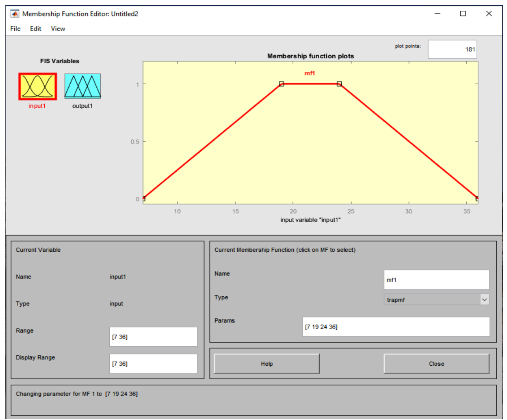
2.3.2. Implementation of First Step of Methodology Using Matlab Program: The Fuzzification of Real Variables Using Four Membership Degree Functions (Four Cases)

The authors calculated the degree of membership of the crisp temperature and humidity values using four membership degree functions (isosceles and scalene triangular and isosceles and random trapezium), which were applied in the new type of fuzzy implications for various values of m. Four different models have been created, which are presented in the picture graphs below.

The following images were extracted from the fuzzy environment of the Matlab program.

First of all, the authors used the Matlab program and applied the following commands on the 122 temperature and humidity values read from excel, respectively:

Temperature = xlsread (“temperature.xls”, 1, “A1:A122”) (Command 1).

Humidity = xlsread (“humidity.xls”, 1, “A1:A122”) (Command 2).

• First Case—Isosceles trapezium (trapezium membership function)

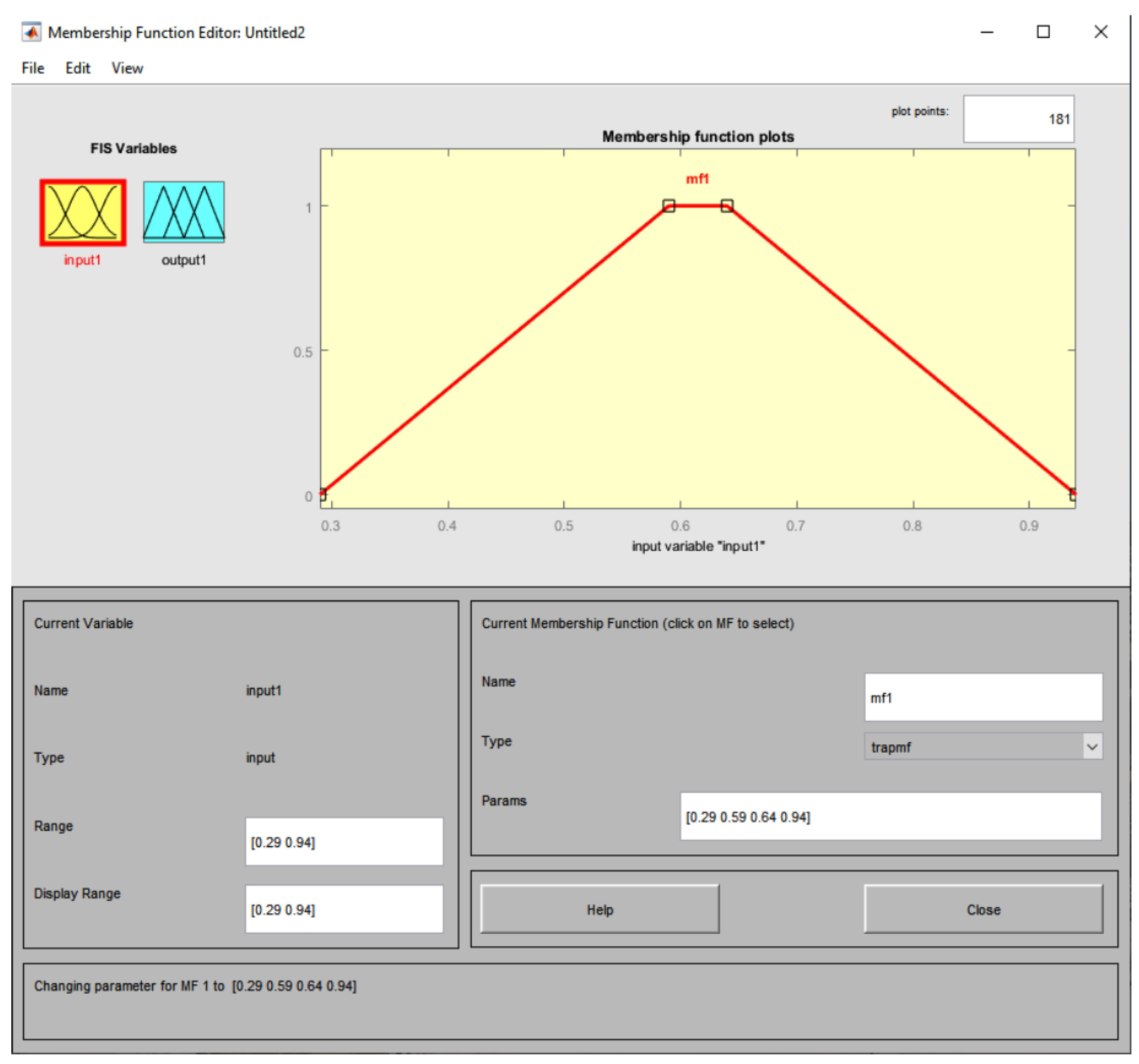
In the first case, the authors used graphs in the form of an isosceles trapezium in a rectangular system of axes with abscissa temperatures or humidities, and the ordinates of the corresponding fuzzy numbers [0, 1]. The vertices of the isosceles trapezoids for temperatures are [7, 19, 24, 36] with graph ordinates [0, 1], while the humidities have the abscissas [0.29, 0.59, 0.64, 0.94] with graph ordinates [0, 1]. The data taken refer to the city of Kavala in Greece and a period of four months—August, September, October and November of the year 2021—and were taken at the same time, 11:50, daily [39] for a total of 122 observations. The value of 7 is the lowest temperature value, and value of 36 is the highest temperature value of all 122 temperature values (all values are derived from 122 observations of temperature). The values 19 and 24 are defined by default in Matlab, as they form the vertices of a trapezium (value 19 is equidistant from 7 and value 24 is equidistant from 36; the sum of 7 and 36 is 43 and the sum of 19 and 24 is 43).

Specifically, the authors typed in the fuzzy command to open the membership function environment. The following command outputs three degrees of membership by fuzzing the temperature values ranging between 7 and 36 based on the vertices of the isosceles trapezium [7, 19, 24, 36] (see Figure 1).

ISOSCELESTRAPEZIUMtemperature = trapmf (temperature, [7, 19, 24, 36]) (Command 3).

Therefore, temperature values greater than 7 and those close to this value will have membership degrees of approximately 0.1 and 0.2, temperature values of 18 and 25 will have a membership degree of approximately 0.9, temperature values between 19 and 24 will have a membership degree of 1, and finally temperature values less than 36 and those close to this value will have membership degrees of about 0.1 and 0.2. Temperature values 7 and 36 have a membership degree of 0.

Command 4 below outputs the membership degrees by fuzzing the humidity values ranging from 0.29 to 0.94, based on the vertices of the isosceles trapezium [0.29, 0.59, 0.64, 0.94] (see Figure 2).

ISOSCELESTRAPEZIUMhumidity = trapmf(humidity, [0.29 0.59 0.64 0.94]) (Command 4).

Therefore, humidity values greater than 0.29 (29%) and those close to this value will have membership degrees of about 0.1 and 0.2, humidity values of 0.57 and 0.58 and 0.65 and 0.66 will have a membership degree of about 0.9, humidity values from 0.59 to 0.64 will have a membership degree of 1, and finally, humidity values smaller than the value 0.94 and close to this value will have degrees of membership of approximately 0.1 and 0.2. Humidity values of 0.29 and 0.94 will have a membership degree of 0. The value of 0.29 (for a percentage of humidity value equal to 29%) is the lowest humidity value, and 0.94 is the highest humidity value of all 122 humidity values (all values are derived from 122 observations of humidity). The values 0.59 and 0.64 are defined by default in Matlab, as they form the vertices of a trapezium (0.59 is equidistant from 0.29 and 0.94 is equidistant from 0.64; the sum of 0.29 and 0.94 is 1.23 and the sum of 0.59 and 0.64 is 1.23).

II.

Second Case—Random trapezium (trapezoidal membership function)

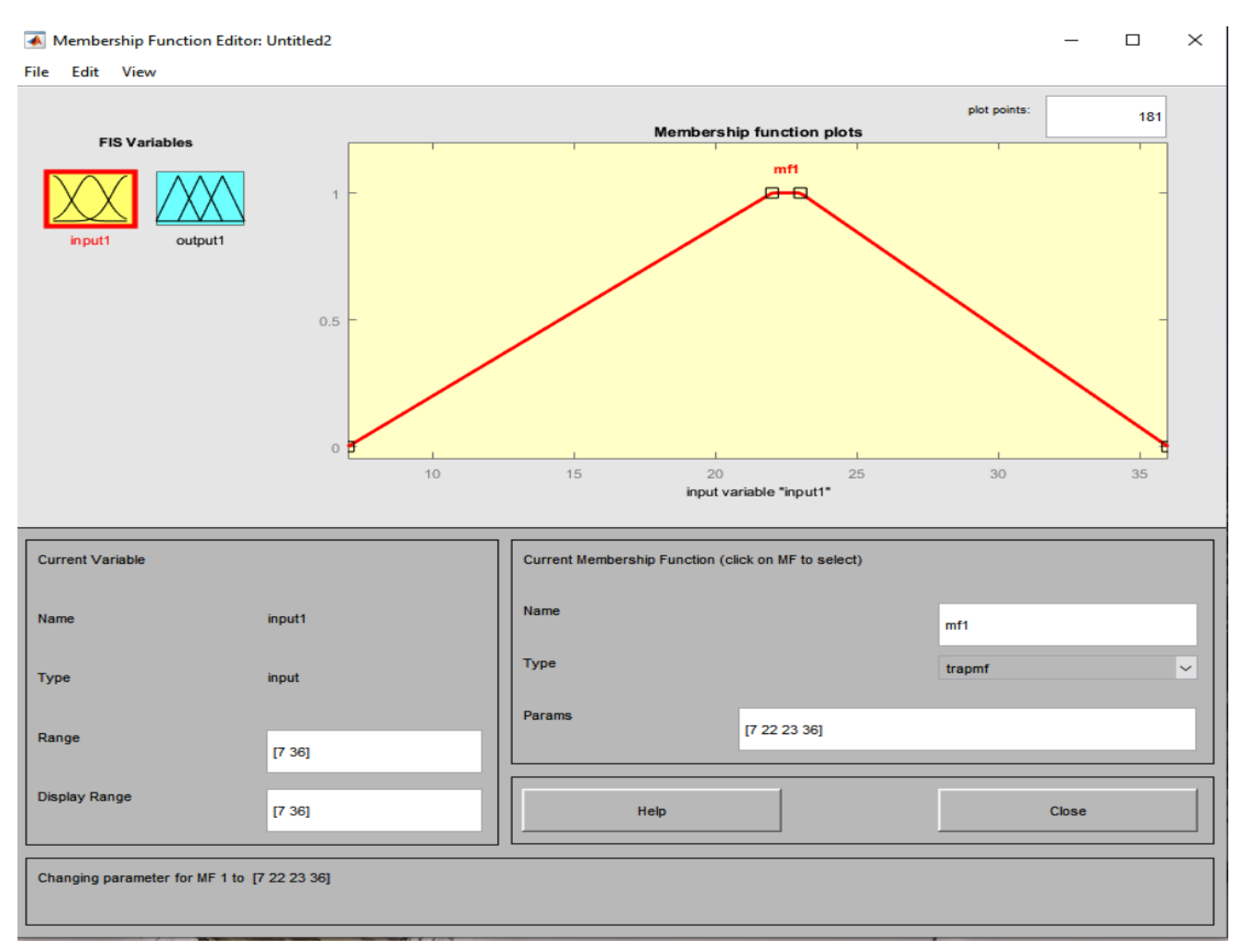
In the second case, the authors construct a random trapezium graph in a rectangular system of axes with abscissas of temperature peaks [7, 22, 23, 36], while the ordinates of the fuzzy corresponding numbers are set as [0, 1] and the humidity values are [0.29, 0.60, 0.61, 0.94], placing the large base on the abscissa axis.

The value of 7 is the lowest temperature value, and 36 is the highest temperature value of all 122 temperature values (all values are derived from 122 observations of temperature). The values 22 and 23 are defined by the authors as vertices of the trapezium for two reasons: The values 22 and 23 appear once each in the entire set of 122 temperature values, and a degree of membership equal to 1 is observed only twice. Secondly, the authors selected a value of 22 because temperature values less than 22 are more frequent (67 values) in the total set of 122 observations.

The value of 0.29 (for a percentage of humidity value equal to 29%) is the lowest humidity value, and 0.94 is the highest humidity value out of all 122 humidity values (all values are derived from 122 observations of humidity). The values 0.60 and 0.61 are defined by the authors as vertices of the trapezium for two reasons: The values 0.60 and 0.61 appear once each in the entire set of 122 humidity values, and the degree of membership of 1 is observed only twice. Secondly, the authors selected the value 0.60 because humidity values less than this value are more common (72 values) in the total set of 122 observations.

Command 5 outputs the membership degrees by fuzzing the temperature values based on the vertices of the random trapezium [7, 22, 23, 36] (see Figure 3).

Command 6 outputs the membership degrees by fuzzing the humidity values based on the vertices of the random trapezium [0.29, 0.60, 0.61, 0.94] (see Figure 4).

RANDOMTRAPEZIUMtemperature = trapmf (thermokrasia, [7, 22, 23, 36]) (Command 5).

RANDOMTRAPEZIUMhumidity = trapmf (humidity, [0.29 0.60 0.61 0.94]) (Command 6).

III.

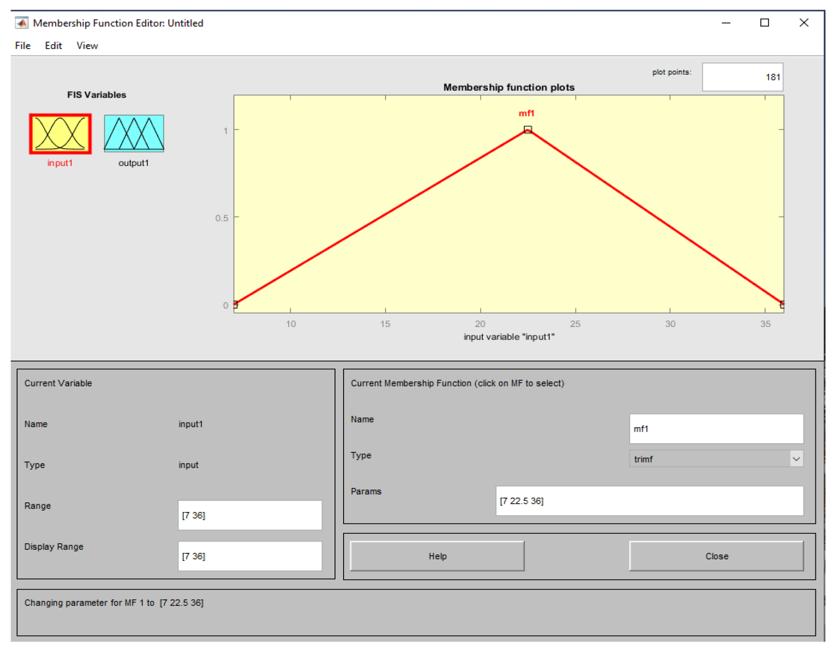
Third Case—Isosceles triangle (triangular membership function)

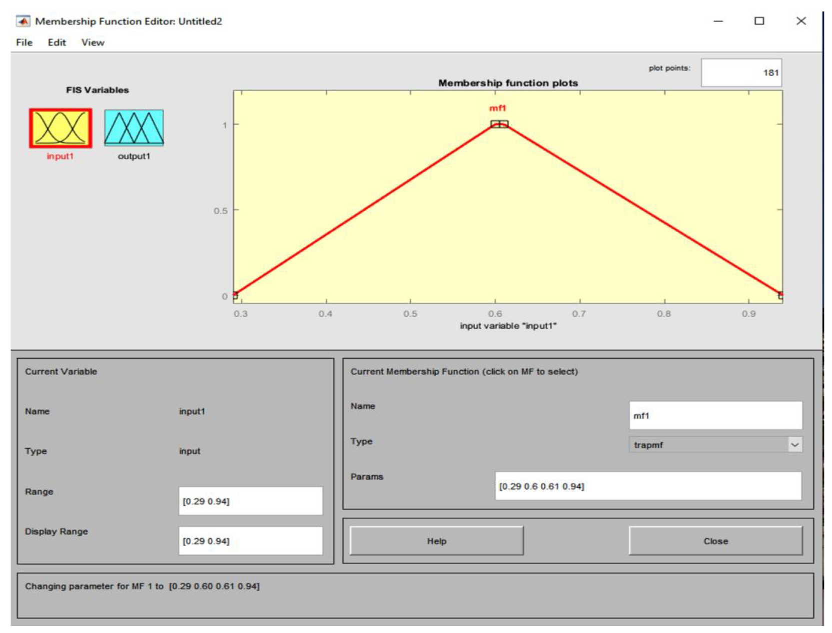
In the third case, we construct an isosceles triangle graph with abscissas of vertices [7, 21.5, 36] and with the base on the axis of the abscissas, while the ordinate of the vertex of the isosceles is set as equal to 1. Similar setting are applied for isosceles triangle humidities with vertices with abscissas of [0.29, 0.615, 0.94] and a maximum ordinate 1, with the base on the abscissa axis.

The value of 7 is the lowest temperature value, and 36 is the highest temperature value of all 122 temperature values (all values are derived from 122 observations of temperature). The value 21.5 is defined as the default by Matlab, as it forms the vertex of the triangle (the value 21.5 is equidistant from 7 and the value 21.5 is equidistant from 36; the sum of 7 and 36 is 43 and it is double 21.5).

The value 0.29 (for a percentage of humidity value equal to 29%) is the lowest humidity value, and 0.94 is the highest humidity value of all 122 humidity values (all values are derived from 122 observations of humidity). The value 0.615 is defined as the default in Matlab, as it forms the vertex of the triangle (the value 0.615 is equidistant from 0.29 and 0.615 is equidistant from 0.94; the sum of 0.29 and 0.94 is 1.23 and it is double 0.615).

Command 7 outputs the membership degrees by fuzzing the temperature values based on the vertices of the isosceles triangle [7, 21.5, 36] (see Figure 5).

Command 8 outputs the membership degrees by fuzzing the humidity values based on the vertices of the isosceles triangle [0.29, 0,615, 0.94] (see Figure 6).

ISOSCELESTRIANGLEtemperature = trimf (temperature, [7, 21.5, 36]) (Command 7).

ISOSCELESTRIANGLEhumidity = trimf (humidity, [0.29 0.615 0.94]) (Command 8).

IV.

Fourth Case—Scalene triangle (triangular membership function)

Finally, in the fourth case, we construct a scalene triangle graph with vertex abscissas [7, 22.5, 36] which are set for the temperature graph and with ordinate values from [0, 1] and an additional scalene triangle with vertex abscissas [0.29, 0.605, 0.94] which are set for the humidity graph and with ordinate values from [0, 1].

The value of 7 is the lowest temperature value and 36 is the highest temperature value of all 122 temperature values (all values are derived from 122 observations of temperature). The value 22.5 is defined by the authors as the form of the vertex of the triangle for two reasons: The value 22.5 does not appear in the set of all 122 temperature values, and a degree of membership equal to 1 is not observed at all. Secondly, the authors selected the value 22.5 because temperature values lower than this are more common (68 cases) in the total set of 122 observations.

The value 0.29 (with a percentage of humidity value equal to 29%) is the lowest humidity value, and 0.94 is the highest humidity value of all 122 humidity values (all values are derived from 122 observations of humidity). The value 0.605 is defined by the authors as the form of the vertex of the triangle for two reasons: The value 0.605 does not appear in the set of all 122 temperature values, and a degree of membership equal to 1 is not observed either. Secondly, the authors selected the value 0.605 because humidity values lower than this are more common (73 cases) in the total set of 122 observations.

Command 9 outputs membership degrees by fuzzing the temperature values based on the vertices of the scalene triangle [7, 22.5, 36] (see Figure 7).

Command 10 outputs membership degrees by fuzzing humidity values based on the vertices of the scalene triangle [0.29, 0.605, 0.94] (see Figure 8).

SCALENETRIANGLEtemperature = trimf (temperature, [7 22.5 36]) (Command 9).

SCALENETRIANGLEhumidity = trimf (humidity, [0.29, 0.605, 0.94]) (Command 10).

3. Results

For cases wherein the degree of membership of temperature = 0, y = 0, and the results of the implications remain stable for each m value. Even for temperature values of 20–24 °C, with small deviations, we derive an almost optimal estimate (the membership degree of temperature is near to or equal to 1), while for the values above 24 °C the estimates are different, with small deviations.

3.1. General Outcomes of Fuzzy Model—The Results from the First Step of the Methodology

The outcome of our fuzzy model is the fuzzification of 122 temperature and 122 humidity crisp values to fuzzy values using the Mamdani Inference System. Using four different membership degree functions (four cases), the authors fuzzified 122 temperature values and 122 humidity values separately, and calculated the corresponding membership degrees in a single fuzzy set, without creating fuzzy rules.

The constructed single fuzzy set does not contain an optimal, mean, or lowest value. In each membership degree function, the single fuzzy set of temperature contains all 122 daily midday temperature crisp values (from 7 to 36) for the city of Kavala over four months as the input, and each is assigned a degree of membership from 0 to 1 as the output. Also, for each membership degree function, the single fuzzy set of humidity contains all 122 daily midday humidity crisp values (from 0.29 to 0.94) for the city of Kavala over four months as input, and each is assigned a degree of membership from 0 to 1 as output.

We used the fuzzy logic designer of the Matlab environment in order to derive fuzzy values of temperature and humidity that could be used in a new type of calculation of fuzzy implication, where variable x represents the degree of membership of humidity values and variable y represents the degree of membership of temperature values.

The purpose of this methodology was not to categorize the values into three linguistic classes οr three fuzzy sets (such as low, medium and high temperature or humidity) and calculate in each of these the degrees of membership. Although this procedure is usually undertaken, in our case the new type of calculation of the fuzzy implication can be tested and evaluated with a single fuzzy set.

For example, take the value 7 (in the value set from 7 to 36), this is the lowest temperature value. If we construct a fuzzy set that will contain all 122 temperature values, the value 7 will have a membership degree equal to 0 (one trapezoidal membership function), in contrast to the three linguistics and three fuzzy sets (one semi-trapezoidal, one trapezoidal and one semi-trapezoidal membership function), wherein the value 7 will belong to the first linguistic (low temperature) with a membership degree equal to 1. Moreover, with three linguistics—low, medium and high values of temperature and humidity—we will find more membership degrees equal to 1. Also, for the value 36 (in the value set from 7 to 36, this is the highest temperature value), if we construct a fuzzy set that will contain all 122 temperature values, this value will have a membership degree equal to 0, in contrast to the situation when using three linguistics and three fuzzy sets, wherein the value 36 will belong to the third linguistic (high temperature) with a membership degree equal to 1.

In an isosceles trapezium, temperature values greater than 7 °C and those close to this value will have membership degrees of approximately 0.1 and 0.2, temperature values of 13 °C and 16 °C will have membership degrees of 0.5 and 0.75, respectively, temperature values of 18 °C and 25 °C will have membership degrees of approximately 0.9, temperature values from 19 °C to 24 °C will have membership degrees of 1, temperature values of 27 °C and 30 °C will have membership degrees of 0.75 and 0.5, respectively, and finally, temperature values less than 36 °C and those close to this value will have membership degrees of about 0.1 and 0.2. Temperature values of 7 °C and 36 °C have membership degrees of 0. Humidity values greater than 0.29 (29%) and those close to this value will have membership degrees of about 0.1 and 0.2, humidity values of 0.44 and 0.5 will have membership degrees of 0.5 and 0.7, respectively, humidity values of 0.57 and 0.58 and 0.65 and 0.66 will have membership degreed of about 0.9, humidity values from 0.59 to 0.64 will have membership degrees of 1, humidity values of 0.73 will have membership degrees of 0.7, and finally humidity values smaller than 0.94 and those close to this value will have degrees of membership of approximately 0.1 and 0.2. Humidity values of 0.29 and 0.94 will have a membership degree of 0. In Appendix A,

Table A1. Temperature and humidity values with corresponding membership degrees using isosceles trapezium as the trapezoidal membership function.

Kavala 11:50 O’Clock Measurement	Temperature/ Membership Degrees	Humidity/ Membership Degrees	Kavala 11:50 O’Clock Measurement	Temperature/ Membership Degrees	Humidity/ Membership Degrees
1 August 2021	34/0.1667	0.41/0.4000	1 October 2021	21/1.0000	0.38/0.3000
2 August 2021	33/0.2500	0.46/0.5667	2 October 2021	21/1.0000	0.38/0.3000
3 August 2021	35/0.0833	0.44/0.5000	3 October 2021	19/1.0000	0.52/0.7667
4 August 2021	33/0.2500	0.49/0.6667	4 October 2021	20/1.0000	0.46/0.5667
5 August 2021	36/0.0000	0.55/0.8667	5 October 2021	20/1.0000	0.49/0.6667
6 August 2021	33/0.2500	0.46/0.5667	6 October 2021	19/1.0000	0.46/0.5667
7 August 2021	29/0.5833	0.37/0.2667	7 October 2021	20/1.0000	0.4/0.3667
8 August 2021	30/0.5000	0.52/0.7667	8 October 2021	15/0.6667	0.88/0.2000
9 August 2021	30/0.5000	0.59/1.0000	9 October 2021	15/0.6667	0.82/0.4000
10 August 2021	32/0.3333	0.63/1.0000	10 October 2021	16/0.7500	0.72/0.7333
11 August 2021	30/0.5000	0.59/1.0000	11 October 2021	16/0.7500	0.94/0.0000
12 August 2021	30/0.5000	0.52/0.7667	12 October 2021	16/0.7500	0.94/0.0000
13 August 2021	30/0.5000	0.49/0.6667	13 October 2021	14/0.5833	0.94/0.0000
14 August 2021	30/0.5000	0.38/0.3000	14 October 2021	13/0.5000	0.88/0.2000
15 August 2021	29/0.5833	0.43/0.4667	15 October 2021	14/0.5833	0.94/0.0000
16 August 2021	30/0.5000	0.46/0.5667	16 October 2021	18/0.9167	0.88/0.2000
17 August 2021	29/0.5833	0.58/0.9667	17 October 2021	18/0.9167	0.73/0.7000
18 August 2021	31/0.4167	0.52/0.7667	18 October 2021	16/0.7500	0.88/0.2000
19 August 2021	25/0.9167	0.74/0.6667	19 October 2021	16/0.7500	0.77/0.5667
20 August 2021	27/0.7500	0.45/0.5333	20 October 2021	18/0.9167	0.49/0.6667
21 August 2021	28/0.6667	0.45/0.5333	21 October 2021	17/0.8333	0.73/0.7000
22 August 2021	29/0.5833	0.48/0.6333	22 October 2021	18/0.9167	0.78/0.5333
23 August 2021	30/0.5000	0.29/0.0000	23 October 2021	19/1.0000	0.73/0.7000
24 August 2021	29/0.5833	0.4/0.3667	24 October 2021	15/0.6667	0.77/0.5667
25 August 2021	28/0.6667	0.51/0.7333	25 October 2021	14/0.5833	0.48/0.6333
26 August 2021	29/0.5833	0.58/0.9667	26 October 2021	15/0.6667	0.45/0.5333
27 August 2021	29/0.5833	0.62/1.0000	27 October 2021	16/0.7500	0.52/0.7667
28 August 2021	29/0.5833	0.62/1.0000	28 October 2021	14/0.5833	0.72/0.7333
29 August 2021	28/0.6667	0.66/0.9333	29 October 2021	16/0.7500	0.45/0.5333
30 August 2021	29/0.5833	0.51/0.7333	30 October 2021	17/0.8333	0.45/0.5333
31 August 2021	28/0.6667	0.55/0.8667	31 October 2021	17/0.8333	0.52/0.7667
1 September 2021	29/0.5833	0.48/0.6333	1 November 2021	17/0.8333	0.68/0.8667
2 September 2021	26/0.8333	0.37/0.2667	2 November 2021	13/0.5000	0.94/0.0000
3 September 2021	25/0.9167	0.39/0.3333	3 November 2021	17/0.8333	0.83/0.3667
4 September 2021	25/0.9167	0.44/0.5000	4 November 2021	21/1.0000	0.57/0.9333
5 September 2021	25/0.9167	0.47/0.6000	5 November 2021	20/1.0000	0.73/0.7000
6 September 2021	25/0.9167	0.39/0.3333	6 November 2021	18/0.9167	0.88/0.2000
7 September 2021	24/1.0000	0.41/0.4000	7 November 2021	18/0.9167	0.83/0.3667
8 September 2021	21/1.0000	0.53/0.8000	8 November 2021	17/0.8333	0.83/0.3667
9 September 2021	22/1.0000	0.57/0.9333	9 November 2021	18/0.9167	0.83/0.3667
10 September 2021	23/1.0000	0.65/0.9667	10 November 2021	14/0.5833	0.55/0.8667
11 September 2021	25/0.9167	0.54/0.8333	11 November 2021	12/0.4167	0.51/0.7333
12 September 2021	27/0.7500	0.42/0.4333	12 November 2021	14/0.5833	0.51/0.7333
13 September 2021	27/0.7500	0.42/0.4333	13 November 2021	13/0.5000	0.63/1.0000
14 September 2021	29/0.5833	0.31/0.0667	14 November 2021	16/0.7500	0.68/0.8667
15 September 2021	27/0.7500	0.45/0.5333	15 November 2021	15/0.6667	0.68/0.8667
16 September 2021	26/0.8333	0.58/0.9667	16 November 2021	15/0.6667	0.55/0.8667
17 September 2021	26/0.8333	0.61/1.0000	17 November 2021	13/0.5000	0.51/0.7333
18 September 2021	27/0.7500	0.62/1.0000	18 November 2021	12/0.4167	0.63/1.0000
19 September 2021	25/0.9167	0.65/0.9667	19 November 2021	11/0.3333	0.77/0.5667
20 September 2021	27/0.7500	0.54/0.8333	20 November 2021	13/0.5000	0.72/0.7333
21 September 2021	24/1.0000	0.65/0.9667	21 November 2021	16/0.7500	0.63/1.0000
22 September 2021	18/0.9167	0.73/0.7000	22 November 2021	11/0.3333	0.88/0.2000
23 September 2021	19/1.0000	0.52/0.7667	23 November 2021	15/0.6667	0.88/0.2000
24 September 2021	20/1.0000	0.49/0.6667	24 November 2021	13/0.5000	0.55/0.8667
25 September 2021	24/1.0000	0.5/0.7000	25 November 2021	11/0.3333	0.54/0.8333
26 September 2021	25/0.9167	0.57/0.9333	26 November 2021	7/0.0000	0.93/0.0333
27 September 2021	25/0.9167	0.47/0.6000	27 November 2021	14/0.5833	0.88/0.2000
28 September 2021	24/1.0000	0.47/0.6000	28 November 2021	16/0.7500	0.83/0.3667
29 September 2021	20/1.0000	0.6/1.0000	29 November 2021	19/1.0000	0.68/0.8667
30 September 2021	21/1.0000	0.46/0.5667	30 November 2021	12/0.4167	0.51/0.7333

, we list the 122 crisp temperature and humidity values with their corresponding membership degrees using an isosceles trapezium as the trapezoidal membership function.

In a random trapezium, temperature values greater than 7 °C and those close to this value will have membership degrees of approximately 0.1 and 0.2, temperature values of 13 °C and 16 °C will have membership degrees of 0.4 and 0.6, respectively, temperature values of 21 °C and 24 °C will have membership degrees of approximately 0.9, temperature values from 22 °C to 23 °C will have membership degrees of 1, temperature values of 27 °C and 30 °C will have membership degrees of 0.69 and 0.46, respectively, and finally, temperature values less than 36 °C and those close to this value will have membership degrees of about 0.1 and 0.2. Temperature values 7 °C and 36 °C will have membership degrees of 0. Humidity values greater than 0.29 (29%) and those close to this value will have membership degrees of about 0.1 and 0.2, humidity values of 0.44 and 0.5 will have membership degrees of 0.48 and 0.68, respectively, humidity values of 0.58 and 0.59 and 0.62 and 0.63 will have membership degrees of about 0.9, temperature values from 0.60 to 0.61 will have membership degrees of 1, humidity values of 0.73 will have membership degrees of 0.64, and finally humidity values smaller than 0.94 and those close to this value will have degrees of membership of approximately 0.1 and 0.2. Humidity values of 0.29 and 0.94 will have membership degrees of 0. In Appendix A, Table A1, we list the 122 crisp temperature and humidity values with their corresponding membership degrees using an isosceles trapezium as the trapezoidal membership function. In Appendix A,

Table A2. Temperature and humidity values with corresponding membership degrees using random trapezium as trapezoidal membership function.

Kavala 11:50 O’Clock Measurement	Temperature/ Membership Degrees	Humidity/ Membership Degrees	Kavala 11:50 O’Clock Measurement	Temperature/ Membership Degrees	Humidity/ Membership Degrees
1 August 2021	34/0.1538	0.41/0.3871	1 October 2021	21/0.9333	0.38/0.2903
2 August 2021	33/0.2308	0.46/0.5484	2 October 2021	21/0.9333	0.38/0.2903
3 August 2021	35/0.0769	0.44/0.4839	3 October 2021	19/0.8000	0.52/0.7419
4 August 2021	33/0.2308	0.49/0.6452	4 October 2021	20/0.8667	0.46/0.5484
5 August 2021	36/0.0000	0.55/0.8387	5 October 2021	20/0.8667	0.49/0.6452
6 August 2021	33/0.2308	0.46/0.5484	6 October 2021	19/0.8000	0.46/0.5484
7 August 2021	29/0.5385	0.37/0.2581	7 October 2021	20/0.8667	0.4/0.3548
8 August 2021	30/0.4615	0.52/0.7419	8 October 2021	15/0.5333	0.88/0.1818
9 August 2021	30/0.4615	0.59/0.9677	9 October 2021	15/0.5333	0.82/0.3636
10 August 2021	32/0.3077	0.63/0.9394	10 October 2021	16/0.6000	0.72/0.6667
11 August 2021	30/0.4615	0.59/0.9677	11 October 2021	16/0.6000	0.94/0.0000
12 August 2021	30/0.4615	0.52/0.7419	12 October 2021	16/0.6000	0.94/0.0000
13 August 2021	30/0.4615	0.49/0.6452	13 October 2021	14/0.4667	0.94/0.0000
14 August 2021	30/0.4615	0.38/0.2903	14 October 2021	13/0.4000	0.88/0.1818
15 August 2021	29/0.5385	0.43/0.4516	15 October 2021	14/0.4667	0.94/0.0000
16 August 2021	30/0.4615	0.46/0.5484	16 October 2021	18/0.7333	0.88/0.1818
17 August 2021	29/0.5385	0.58/0.9355	17 October 2021	18/0.7333	0.73/0.6364
18 August 2021	31/0.3846	0.52/0.7419	18 October 2021	16/0.6000	0.88/0.1818
19 August 2021	25/0.8462	0.74/0.6061	19 October 2021	16/0.6000	0.77/0.5152
20 August 2021	27/0.6923	0.45/0.5161	20 October 2021	18/0.7333	0.49/0.6452
21 August 2021	28/0.6154	0.45/0.5161	21 October 2021	17/0.6667	0.73/0.6364
22 August 2021	29/0.5385	0.48/0.6129	22 October 2021	18/0.7333	0.78/0.4848
23 August 2021	30/0.4615	0.29/0.0000	23 October 2021	19/0.8000	0.73/0.6364
24 August 2021	29/0.5385	0.4/0.3548	24 October 2021	15/0.5333	0.77/0.5152
25 August 2021	28/0.6154	0.51/0.7097	25 October 2021	14/0.4667	0.48/0.6129
26 August 2021	29/0.5385	0.58/0.9355	26 October 2021	15/0.5333	0.45/0.5161
27 August 2021	29/0.5385	0.62/0.9697	27 October 2021	16/0.6000	0.52/0.7419
28 August 2021	29/0.5385	0.62/0.9697	28 October 2021	14/0.4667	0.72/0.6667
29 August 2021	28/0.6154	0.66/0.8485	29 October 2021	16/0.6000	0.45/0.5161
30 August 2021	29/0.5385	0.51/0.7097	30 October 2021	17/0.6667	0.45/0.5161
31 August 2021	28/0.6154	0.55/0.8387	31 October 2021	17/0.6667	0.52/0.7419
1 September 2021	29/0.5385	0.48/0.6129	1 November 2021	17/0.6667	0.68/0.7879
2 September 2021	26/0.7692	0.37/0.2581	2 November 2021	13/0.4000	0.94/0.0000
3 September 2021	25/0.8462	0.39/0.3226	3 November 2021	17/0.6667	0.83/0.3333
4 September 2021	25/0.8462	0.44/0.4839	4 November 2021	21/0.9333	0.57/0.9032
5 September 2021	25/0.8462	0.47/0.5806	5 November 2021	20/0.8667	0.73/0.6364
6 September 2021	25/0.8462	0.39/0.3226	6 November 2021	18/0.7333	0.88/0.1818
7 September 2021	24/0.9231	0.41/0.3871	7 November 2021	18/0.7333	0.83/0.3333
8 September 2021	21/0.9333	0.53/0.7742	8 November 2021	17/0.6667	0.83/0.3333
9 September 2021	22/1.0000	0.57/0.9032	9 November 2021	18/0.7333	0.83/0.3333
10 September 2021	23/1.0000	0.65/0.8788	10 November 2021	14/0.4667	0.55/0.8387
11 September 2021	25/0.8462	0.54/0.8065	11 November 2021	12/0.3333	0.51/0.7097
12 September 2021	27/0.6923	0.42/0.4194	12 November 2021	14/0.4667	0.51/0.7097
13 September 2021	27/0.6923	0.42/0.4194	13 November 2021	13/0.4000	0.63/0.9394
14 September 2021	29/0.5385	0.31/0.0645	14 November 2021	16/0.6000	0.68/0.7879
15 September 2021	27/0.6923	0.45/0.5161	15 November 2021	15/0.5333	0.68/0.7879
16 September 2021	26/0.7692	0.58/0.9355	16 November 2021	15/0.5333	0.55/0.8387
17 September 2021	26/0.7692	0.61/1.0000	17 November 2021	13/0.4000	0.51/0.7097
18 September 2021	27/0.6923	0.62/0.9697	18 November 2021	12/0.3333	0.63/0.9394
19 September 2021	25/0.8462	0.65/0.8788	19 November 2021	11/0.2667	0.77/0.5152
20 September 2021	27/0.6923	0.54/0.8065	20 November 2021	13/0.4000	0.72/0.6667
21 September 2021	24/0.9231	0.65/0.8788	21 November 2021	16/0.6000	0.63/0.9394
22 September 2021	18/0.7333	0.73/0.6364	22 November 2021	11/0.2667	0.88/0.1818
23 September 2021	19/0.8000	0.52/0.7419	23 November 2021	15/0.5333	0.88/0.1818
24 September 2021	20/0.8667	0.49/0.6452	24 November 2021	13/0.4000	0.55/0.8387
25 September 2021	24/0.9231	0.5/0.6774	25 November 2021	11/0.2667	0.54/0.8065
26 September 2021	25/0.8462	0.57/0.9032	26 November 2021	7/0.0000	0.93/0.0303
27 September 2021	25/0.8462	0.47/0.5806	27 November 2021	14/0.4667	0.88/0.1818
28 September 2021	24/0.9231	0.47/0.5806	28 November 2021	16/0.6000	0.83/0.3333
29 September 2021	20/0.8667	0.6/1.0000	29 November 2021	19/0.8000	0.68/0.7879
30 September 2021	21/0.9333	0.46/0.5484	30 November 2021	12/0.3333	0.51/0.7097

, we list the 122 crisp temperature and humidity values with their corresponding membership degrees using random trapezium as the trapezoidal membership function.

In isosceles triangles, temperature values greater than 7 °C and those close to this value will have membership degrees of approximately 0.1 and 0.2, temperature values of 13 °C and 16 °C will have membership degrees of 0.41 and 0.62, respectively, temperature values of 20 °C and 23 °C will have membership degrees of approximately 0.9, temperature values of 21 °C and 22 °C will have membership degrees of approximately 1, temperature values of 27 °C and 30 °C will have membership degrees of 0.62 and 0.41, respectively, and finally temperature values less than 36 °C and those close to this value will have membership degrees of about 0.1 and 0.2. Temperature values of 7 °C and 36 °C have membership degrees of 0. Humidity values greater than 0.29 (29%) and those close to this value will have membership degrees of about 0.1 and 0.2, humidity values of 0.44 and 0.5 will have membership degrees of 0.46 and 0.65, respectively, humidity values of 0.57, 0.58, 0.59, 0.6, 0.61, 0.64, 0.65 and 0.66 will have membership degrees of about 0.9, humidity values from 0.62 to 0.63 will have membership degrees of approximately 1, humidity values of 0.73 will have membership degreed of 0.65, and finally humidity values smaller than 0.94 and those close to this value will have degrees of membership of approximately 0.1 and 0.2. Humidity values of 0.29 and 0.94 have membership degrees of 0. In Appendix A,

Table A3. Temperature and humidity values with corresponding membership degrees using isosceles triangle as triangular membership function.

Kavala 11:50 O’Clock Measurement	Temperature/ Membership Degrees	Humidity/ Membership Degrees	Kavala 11:50 O’Clock Measurement	Temperature/ Membership Degrees	Humidity/ Membership Degrees
1 August 2021	34/0.1379	0.41/0.3692	1 October 2021	21/0.9655	0.38/0.2769
2 August 2021	33/0.2069	0.46/0.5231	2 October 2021	21/0.9655	0.38/0.2769
3 August 2021	35/0.0690	0.44/0.4615	3 October 2021	19/0.8276	0.52/0.7077
4 August 2021	33/0.2069	0.49/0.6154	4 October 2021	20/0.8966	0.46/0.5231
5 August 2021	36/0.0000	0.55/0.8000	5 October 2021	20/0.8966	0.49/0.6154
6 August 2021	33/0.2069	0.46/0.5231	6 October 2021	19/0.8276	0.46/0.5231
7 August 2021	29/0.4828	0.37/0.2462	7 October 2021	20/0.8966	0.4/0.3385
8 August 2021	30/0.4138	0.52/0.7077	8 October 2021	15/0.5517	0.88/0.1846
9 August 2021	30/0.4138	0.59/0.9231	9 October 2021	15/0.5517	0.82/0.3692
10 August 2021	32/0.2759	0.63/0.9538	10 October 2021	16/0.6207	0.72/0.6769
11 August 2021	30/0.4138	0.59/0.9231	11 October 2021	16/0.6207	0.94/0.0000
12 August 2021	30/0.4138	0.52/0.7077	12 October 2021	16/0.6207	0.94/0.0000
13 August 2021	30/0.4138	0.49/0.6154	13 October 2021	14/0.4828	0.94/0.0000
14 August 2021	30/0.4138	0.38/0.2769	14 October 2021	13/0.4138	0.88/0.1846
15 August 2021	29/0.4828	0.43/0.4308	15 October 2021	14/0.4828	0.94/0.0000
16 August 2021	30/0.4138	0.46/0.5231	16 October 2021	18/0.7586	0.88/0.1846
17 August 2021	29/0.4828	0.58/0.8923	17 October 2021	18/0.7586	0.73/0.6462
18 August 2021	31/0.3448	0.52/0.7077	18 October 2021	16/0.6207	0.88/0.1846
19 August 2021	25/0.7586	0.74/0.6154	19 October 2021	16/0.6207	0.77/0.5231
20 August 2021	27/0.6207	0.45/0.4923	20 October 2021	18/0.7586	0.49/0.6154
21 August 2021	28/0.5517	0.45/0.4923	21 October 2021	17/0.6897	0.73/0.6462
22 August 2021	29/0.4828	0.48/0.5846	22 October 2021	18/0.7586	0.78/0.4923
23 August 2021	30/0.4138	0.29/0.0000	23 October 2021	19/0.8276	0.73/0.6462
24 August 2021	29/0.4828	0.4/0.3385	24 October 2021	15/0.5517	0.77/0.5231
25 August 2021	28/0.5517	0.51/0.6769	25 October 2021	14/0.4828	0.48/0.5846
26 August 2021	29/0.4828	0.58/0.8923	26 October 2021	15/0.5517	0.45/0.4923
27 August 2021	29/0.4828	0.62/0.9846	27 October 2021	16/0.6207	0.52/0.7077
28 August 2021	29/0.4828	0.62/0.9846	28 October 2021	14/0.4828	0.72/0.6769
29 August 2021	28/0.5517	0.66/0.8615	29 October 2021	16/0.6207	0.45/0.4923
30 August 2021	29/0.4828	0.51/0.6769	30 October 2021	17/0.6897	0.45/0.4923
31 August 2021	28/0.5517	0.55/0.8000	31 October 2021	17/0.6897	0.52/0.7077
1 September 2021	29/0.4828	0.48/0.5846	1 November 2021	17/0.6897	0.68/0.8000
2 September 2021	26/0.6897	0.37/0.2462	2 November 2021	13/0.4138	0.94/0.0000
3 September 2021	25/0.7586	0.39/0.3077	3 November 2021	17/0.6897	0.83/0.3385
4 September 2021	25/0.7586	0.44/0.4615	4 November 2021	21/0.9655	0.57/0.8615
5 September 2021	25/0.7586	0.47/0.5538	5 November 2021	20/0.8966	0.73/0.6462
6 September 2021	25/0.7586	0.39/0.3077	6 November 2021	18/0.7586	0.88/0.1846
7 September 2021	24/0.8276	0.41/0.3692	7 November 2021	18/0.7586	0.83/0.3385
8 September 2021	21/0.9655	0.53/0.7385	8 November 2021	17/0.6897	0.83/0.3385
9 September 2021	22/0.9655	0.57/0.8615	9 November 2021	18/0.7586	0.83/0.3385
10 September 2021	23/0.8966	0.65/0.8923	10 November 2021	14/0.4828	0.55/0.8000
11 September 2021	25/0.7586	0.54/0.7692	11 November 2021	12/0.3448	0.51/0.6769
12 September 2021	27/0.6207	0.42/0.4000	12 November 2021	14/0.4828	0.51/0.6769
13 September 2021	27/0.6207	0.42/0.4000	13 November 2021	13/0.4138	0.63/0.9538
14 September 2021	29/0.4828	0.31/0.0615	14 November 2021	16/0.6207	0.68/0.8000
15 September 2021	27/0.6207	0.45/0.4923	15 November 2021	15/0.5517	0.68/0.8000
16 September 2021	26/0.6897	0.58/0.8923	16 November 2021	15/0.5517	0.55/0.8000
17 September 2021	26/0.6897	0.61/0.9846	17 November 2021	13/0.4138	0.51/0.6769
18 September 2021	27/0.6207	0.62/0.9846	18 November 2021	12/0.3448	0.63/0.9538
19 September 2021	25/0.7586	0.65/0.8923	19 November 2021	11/0.2759	0.77/0.6769
20 September 2021	27/0.6207	0.54/0.7692	20 November 2021	13/0.4138	0.72/0.9538
21 September 2021	24/0.8276	0.65/0.8923	21 November 2021	16/0.6207	0.63/0.9538
22 September 2021	18/0.7586	0.73/0.6462	22 November 2021	11/0.2759	0.88/0.1846
23 September 2021	19/0.8276	0.52/0.7077	23 November 2021	15/0.5517	0.88/0.1846
24 September 2021	20/0.8966	0.49/0.6154	24 November 2021	13/0.4138	0.55/0.8000
25 September 2021	24/0.8276	0.5/0.6462	25 November 2021	11/0.2759	0.54/0.7692
26 September 2021	25/0.7586	0.57/0.8615	26 November 2021	7/0.0000	0.93/0.0308
27 September 2021	25/0.7586	0.47/0.5538	27 November 2021	14/0.4828	0.88/0.1846
28 September 2021	24/0.8276	0.47/0.5538	28 November 2021	16/0.6207	0.83/0.3385
29 September 2021	20/0.8966	0.6/0.9538	29 November 2021	19/0.8276	0.68/0.8000
30 September 2021	21/0.9655	0.46/0.5231	30 November 2021	12/0.3448	0.51/0.6769

, the 122 crisp temperature and humidity values along with their corresponding membership degrees have been calculated using the isosceles triangle as the triangular membership function.

In a scalene triangle, temperature values greater than 7 °C and those close to this value will have membership degrees of approximately 0.1 and 0.2, temperature values of 13 °C and 16 °C will have membership degrees of 0.39 and 0.58, respectively, temperature values of 21 °C and 24 °C will have membership degrees of approximately 0.9, temperature values of 22 °C and 23 °C will have membership degrees of approximately 1, temperature values of 27 °C and 30 °C will have membership degrees of 0.67 and 0.44, respectively, and finally, temperature values less than 36 °C and those close to this value will have membership degrees of about 0.1 and 0.2. Temperature values of 7 °C and 36 °C will have a membership degree of 0. Humidity values greater than 0.29 (29%) and those close to this value will have membership degrees of about 0.1 and 0.2, humidity values of 0.44 and 0.5 will have membership degrees of 0.48 and 0.67, respectively, humidity values of 0.58 and 0.59 and 0.62 and 0.63 will have membership degrees of about 0.9, humidity values of 0.6 and 0.61 will have membership degrees of approximately 1, humidity values of 0.73 will have membership degrees of 0.63, and finally, humidity values lower than 0.94 and those close to this value will have degrees of membership of approximately 0.1 and 0.2. Humidity values of 0.29 and 0.94 will have membership degrees of 0. In Appendix A,

Table A4. Temperature and humidity values with corresponding membership degrees using scalene triangle as triangular membership function.

Kavala 11:50 O’Clock Measurement	Temperature/ Membership Degrees	Humidity/ Membership Degrees	Kavala 11:50 O’Clock Measurement	Temperature/ Membership Degrees	Humidity/ Membership Degrees
1 August 2021	34/0.1481	0.41/0.3810	1 October 2021	21/0.9032	0.38/0.2857
2 August 2021	33/0.2222	0.46/0.5397	2 October 2021	21/0.9032	0.38/0.2857
3 August 2021	35/0.0741	0.44/0.4762	3 October 2021	19/0.7742	0.52/0.7302
4 August 2021	33/0.2222	0.49/0.6349	4 October 2021	20/0.8387	0.46/0.5397
5 August 2021	36/0.0000	0.55/0.8254	5 October 2021	20/0.8387	0.49/0.6349
6 August 2021	33/0.2222	0.46/0.5397	6 October 2021	19/0.7742	0.46/0.5397
7 August 2021	29/0.5185	0.37/0.2540	7 October 2021	20/0.8387	0.4/0.3492
8 August 2021	30/0.4444	0.52/0.7302	8 October 2021	15/0.5161	0.88/0.1791
9 August 2021	30/0.4444	0.59/0.9524	9 October 2021	15/0.5161	0.82/0.3582
10 August 2021	32/0.2963	0.63/0.9254	10 October 2021	16/0.5806	0.72/0.6567
11 August 2021	30/0.4444	0.59/0.9524	11 October 2021	16/0.5806	0.94/0.0000
12 August 2021	30/0.4444	0.52/0.7302	12 October 2021	16/0.5806	0.94/0.0000
13 August 2021	30/0.4444	0.49/0.6349	13 October 2021	14/0.4516	0.94/0.0000
14 August 2021	30/0.4444	0.38/0.2857	14 October 2021	13/0.3871	0.88/0.1791
15 August 2021	29/0.5185	0.43/0.4444	15 October 2021	14/0.4516	0.94/0.0000
16 August 2021	30/0.4444	0.46/0.5397	16 October 2021	18/0.7097	0.88/0.1791
17 August 2021	29/0.5185	0.58/0.9206	17 October 2021	18/0.7097	0.73/0.6269
18 August 2021	31/0.3704	0.52/0.7302	18 October 2021	16/0.5806	0.88/0.1791
19 August 2021	25/0.8148	0.74/0.5970	19 October 2021	16/0.5806	0.77/0.5075
20 August 2021	27/0.6667	0.45/0.5079	20 October 2021	18/0.7097	0.49/0.6349
21 August 2021	28/0.5926	0.45/0.5079	21 October 2021	17/0.6452	0.73/0.6269
22 August 2021	29/0.5185	0.48/0.6032	22 October 2021	18/0.7097	0.78/0.4776
23 August 2021	30/0.4444	0.29/0.0000	23 October 2021	19/0.7742	0.73/0.6269
24 August 2021	29/0.5185	0.4/0.3492	24 October 2021	15/0.5161	0.77/0.5075
25 August 2021	28/0.5926	0.51/0.6984	25 October 2021	14/0.4516	0.48/0.6032
26 August 2021	29/0.5185	0.58/0.9206	26 October 2021	15/0.5161	0.45/0.5079
27 August 2021	29/0.5185	0.62/0.9552	27 October 2021	16/0.5806	0.52/0.7302
28 August 2021	29/0.5185	0.62/0.9552	28 October 2021	14/0.4516	0.72/0.6567
29 August 2021	28/0.5926	0.66/0.8358	29 October 2021	16/0.5806	0.45/0.5079
30 August 2021	29/0.5185	0.51/0.6984	30 October 2021	17/0.6452	0.45/0.5079
31 August 2021	28/0.5926	0.55/0.8254	31 October 2021	17/0.6452	0.52/0.7302
1 September 2021	29/0.5185	0.48/0.6032	1 November 2021	17/0.6452	0.68/0.7761
2 September 2021	26/0.7407	0.37/0.2540	2 November 2021	13/0.3871	0.94/0.0000
3 September 2021	25/0.8148	0.39/0.3175	3 November 2021	17/0.6452	0.83/0.3284
4 September 2021	25/0.8148	0.44/0.4762	4 November 2021	21/0.9032	0.57/0.8889
5 September 2021	25/0.8148	0.47/0.5714	5 November 2021	20/0.8387	0.73/0.6269
6 September 2021	25/0.8148	0.39/0.3175	6 November 2021	18/0.7097	0.88/0.1791
7 September 2021	24/0.8889	0.41/0.3810	7 November 2021	18/0.7097	0.83/0.3284
8 September 2021	21/0.9032	0.53/0.7619	8 November 2021	17/0.6452	0.83/0.3284
9 September 2021	22/0.9677	0.57/0.8889	9 November 2021	18/0.7097	0.83/0.3284
10 September 2021	23/0.9630	0.65/0.8657	10 November 2021	14/0.4516	0.55/0.8254
11 September 2021	25/0.8148	0.54/0.7937	11 November 2021	12/0.3226	0.51/0.6984
12 September 2021	27/0.6667	0.42/0.4127	12 November 2021	14/0.4516	0.51/0.6984
13 September 2021	27/0.6667	0.42/0.4127	13 November 2021	13/0.3871	0.63/0.9254
14 September 2021	29/0.5185	0.31/0.0635	14 November 2021	16/0.5806	0.68/0.7761
15 September 2021	27/0.6667	0.45/0.5079	15 November 2021	15/0.5161	0.68/0.7761
16 September 2021	26/0.7407	0.58/0.9206	16 November 2021	15/0.5161	0.55/0.8254
17 September 2021	26/0.7407	0.61/0.9851	17 November 2021	13/0.3871	0.51/0.6984
18 September 2021	27/0.6667	0.62/0.9552	18 November 2021	12/0.3226	0.63/0.9254
19 September 2021	25/0.8148	0.65/0.8657	19 November 2021	11/0.2581	0.77/0.5075
20 September 2021	27/0.6667	0.54/0.7937	20 November 2021	13/0.3871	0.72/0.6567
21 September 2021	24/0.8889	0.65/0.8657	21 November 2021	16/0.5806	0.63/0.9254
22 September 2021	18/0.7097	0.73/0.6269	22 November 2021	11/0.2581	0.88/0.1791
23 September 2021	19/0.7742	0.52/0.7302	23 November 2021	15/0.5161	0.88/0.1791
24 September 2021	20/0.8387	0.49/0.6349	24 November 2021	13/0.3871	0.55/0.8254
25 September 2021	24/0.8889	0.5/0.6667	25 November 2021	11/0.2581	0.54/0.7937
26 September 2021	25/0.8148	0.57/0.8889	26 November 2021	7/0.0000	0.93/0.0299
27 September 2021	25/0.8148	0.47/0.5714	27 November 2021	14/0.4516	0.88/0.1791
28 September 2021	24/0.8889	0.47/0.5714	28 November 2021	16/0.5806	0.83/0.3284
29 September 2021	20/0.8387	0.6/0.9841	29 November 2021	19/0.7742	0.68/0.7761
30 September 2021	21/0.9032	0.46/0.5397	30 November 2021	12/0.3226	0.51/0.6984

, we list the 122 crisp temperature and humidity values with their corresponding membership degrees, calculated using the scalene triangle as the triangular membership function.

Moreover, the outcomes of the fuzzy model (the fuzzification of 122 temperature and 122 humidity crisp values to fuzzy values) help us determine in each membership degree function: (a) the number of repetitions (the value of m) needed to ensure that the new fuzzy implication will take the optimal value 1 and a value greater than or equal to 0.9 (third step of methodology); (b) the numbers of temperature and humidity pairs wherein the fuzzy implication takes the optimal value 1 and a value greater than or equal to $0.9$ (fourth step of methodology), based on the calculated value of m or the calculated number of repetitions; and (c) which membership degree function gives the best results in the third and the fourth steps of the methodology.

3.2. General Outcomes of Fuzzy Model—The Results from the Second Step of the Methodology

Based on step 1 in the previous subsection, we can make the following observations.

Ιn the isosceles trapezium, 11 crisp values of humidity (variable x) reached a membership degree equal to 1, and 22 crisp values of temperature (variable y) received a membership degree equal to 1. Also, six crisp values of humidity received a membership degree equal to 0 and two crisp values of temperature received a membership degree equal to 0. When variable y has a membership degree equal to 1, the new type of fuzzy implication takes the value 1 from the first repetition; this pertains when the value of m is equal to 1 and regardless of the membership degree of the variable x. When variable x has a membership degree equal to 0, the new type of fuzzy implication takes the value 1 from the first repetition; this pertains when the value of m is equal to 1, regardless of the membership degree of the variable y. Also, when variables y and x have a membership degree equal to 1, the new type of fuzzy implication takes the value 1 from the first repetition, and this pertains when the value of m is equal to 1.

In the random trapezium, two crisp values of humidity received a membership degree equal to 1, and 2 crisp values of temperature received a membership degree equal to 1. Also, six crisp values of humidity received a membership degree equal to 0 and two crisp values of temperature received a membership degree equal to 0.

Ιn the isosceles and scalene triangles, 0 crisp values of humidity received a membership degree equal to 1 and 0 crisp values of temperature received a membership degree equal to 1. Also, six crisp values of humidity received a membership degree equal to 0 and two crisp values of temperature received a membership degree equal to 0.

In all four cases, the same crisp values of humidity and temperature (minimum and maximum values) received a membership degree equal to 0.

3.3. General Outcomes of Fuzzy Model—The Results from the Third Step of the Methodology

Firstly, the authors observed that in the isosceles trapezium (first model), the new fuzzy implication takes a value greater than or equal to $0.9$, with 19 repetitions of the value of m. Also, the researchers found that in the isosceles trapezium, the new fuzzy implication takes a value equal to $1$, with 239 repetitions of the value of m (see

Table 1. Values of fuzzy implication (Equation (1)) for case I and case II.

	Value m	Case I 1	Case II 2
$\mathit{n}\left(\mathit{x}\right)\mathit{V}{\widehat{\mathbf{y}}}^{\mathit{m}}$
$\ge 0.9$		19	20
$=1$		239	259

¹ Case I: Isosceles trapezium. ² Case II: Random trapezium.

).

Secondly, the authors point out that in the random trapezium (second model), the new fuzzy implication takes a value greater than or equal to $0.9$ with 20 repetitions of the value of m. Also, the researchers observed that in the random trapezium, the new fuzzy implication takes a value equal to $1$, with 259 repetitions of the value of m (see Table 1).

Moreover, the authors observed that in the isosceles triangle (third model), the new fuzzy implication takes a value greater than or equal to $0.9$ with 22 repetitions of the value of m. In this model, we can see that in the isosceles triangle, the new fuzzy implication takes a value equal to $1$, with 289 repetitions of the value of m (see

Table 2. Values of fuzzy implication (Equation (1)) for case III and case IV.

	Value m	Case III 3	Case IV 4
$\mathit{n}\left(\mathit{x}\right)\mathit{V}{\widehat{\mathbf{y}}}^{\mathit{m}}$
$\ge 0.9$		22	21
$=1$		289	269

³ Case III: Isosceles triangle. ⁴ Case IV: Scalene triangle.

).

Also, the authors point out that in the scalene triangle (fourth model), the new fuzzy implication takes a value greater than or equal to $0.9$, with 21 repetitions of the value of m. In this model, we found that in the scalene triangle, the new fuzzy implication takes a value equal to $1$, with 269 repetitions of the value of m (see Table 2).

In the first model, the value of m requires fewer repetitions, meaning that the new fuzzy implication takes a value greater than or equal to $0.9$, or an optimal value equal to $1$, in contrast with the third model, which needs more repetitions of the value of m. The first model is the best solution, and the third model is the worst option.

3.4. General Outcomes of Fuzzy Model—The Results from the Fourth Step of the Methodology

In

Table 3. The number of temperature–humidity pairs where the new fuzzy implication takes the value $\ge 0.9$ and the optimal value $=1$ in case I—isosceles trapezium.

	Value m	Case I with 19 Repetitions	Case I with 239 Repetitions
$\mathit{n}\left(\mathit{x}\right)\mathit{V}{\widehat{\mathbf{y}}}^{\mathit{m}}$
$\ge 0.9$		47	1
$=1$		74	120

, it is clearly visible that in case I of the isosceles trapezium, in the 19th repetition, 74 temperature–humidity pairs of corollaries from the total set of 122 values received the value 1. Moreover, it was observed that, in the isosceles trapezium, in the 19th repetition, only 47 temperature–humidity pairs of corollaries in the total set of 122 values received values $\ge 0.9$ and <1. Also, in the isosceles trapezium, in the 239th repetition, 120 temperature–humidity pairs received the value 1.

In

Table 4. The number of temperature–humidity pairs wherein the new fuzzy implication takes the value $\ge 0.9$ and the optimal value $=1$ in case II—random trapezium.

	Value m	Case II with 20 Repetitions	Case II with 259 Repetitions
$\mathit{n}\left(\mathit{x}\right)\mathit{V}{\widehat{\mathbf{y}}}^{\mathit{m}}$
$\ge 0.9$		61	1
$=1$		60	120

, it is clearly visible that for case II of a random trapezium, in the 20th repetition, only 60 temperature–humidity pairs received the value 1. Moreover, it was observed that in the random trapezium, in the 20th repetition, 61 temperature–humidity pairs received values ≥0.9 and <1. Also, in the random trapezium, in the 259th repetition, 120 temperature–humidity pairs received the value 1.

In

Table 5. The number of temperature–humidity pairs wherein the new fuzzy implication takes the value $\ge 0.9$ and the optimal value $=1$ in case III—isosceles triangle.

	Value m	Case III with 22 Repetitions	Case III with 289 Repetitions
$\mathit{n}\left(\mathit{x}\right)\mathit{V}{\widehat{\mathbf{y}}}^{\mathit{m}}$
$\ge 0.9$		55	1
$=1$		66	120

, it is clearly visible that in case III of the isosceles triangle, in the 22nd repetition, 66 temperature–humidity pairs received the value 1. Moreover, it was observed that in the isosceles triangle, in the 22nd repetition, 55 temperature–humidity pairs received values $\ge 0.9$ and <1. Also, in the isosceles triangle, in the 289th repetition, 120 temperature–humidity pairs received the value 1.

In

Table 6. The number of temperature–humidity pairs wherein the new fuzzy implication takes the value $\ge 0.9$ and the optimal value =1 in case IV—scalene triangle.

	Value m	Case IV with 21 Repetitions	Case IV with 269 Repetitions
$\mathit{n}\left(\mathit{x}\right)\mathit{V}{\widehat{\mathbf{y}}}^{\mathit{m}}$
$\ge 0.9$		61	1
$=1$		60	120

, it is clearly visible that in case IV of the scalene triangle, in the 21st repetition, only 60 temperature–humidity pairs received the value 1. Moreover, it was observed that in the scalene triangle, in the 21st repetition, 61 temperature–humidity pairs received values $\ge 0.9$ and <1. Also, in the scalene triangle, in the 269th repetition, 120 temperature–humidity pairs received the value 1.

With the random trapezium, isosceles and scalene triangles, fewer pairs of temperature and humidity values received a value of 1, with both the random trapezium (with 20 repetitions) and the scalene triangle (with 21 repetitions) receiving a worse result (see Table 4, Table 5 and Table 6). Also, the random trapezium and scalene triangles gave the most pairs (61) of temperature–humidity results in the total set of 122 values that received a value equal to or above 0.9, but not a value equal to 1 (see Table 4 and Table 6).

It therefore follows that the isosceles trapezium gave the best results (more pairs of temperature and humidity values that received a value equal to 1) in relation to the other cases, and they did so in shorter times (fewer repetitions, 19 repetitions).

Moreover, the isosceles trapezium compared to the rest of the models derived the optimal values in a shorter time, and specifically, 120 temperature–humidity pairs received a value of 1 at the 239th repetition (out of the total of 122 values) (see Table 3). The other models required more repetitions to achieve the same result (120 pairs of temperature and humidity values), with the third model (case III) needing the most (289) repetitions.

Only one pair of temperature and humidity values (from the total set of 122 pairs) failed to reach a value greater than or equal to 0.9 for all four membership degree functions.

4. Discussion

In this paper, the authors have proposed a new type of fuzzy implication using the axioms and theorems of fuzzy logic, which has proven to be very reliable and useful for the science of mathematics and Soft Computing. Secondly, the authors fuzzified 122 temperature and humidity values using four membership degree functions so as to find the degree of membership of the 122 values for each membership degree function. In the third stage, the membership degrees of the temperature and humidity values were applied to the new type of fuzzy implication (Equation (16)). In this formula, variable x represents the degree of membership of humidity values, and variable y represents the degree of membership of temperature values. After this, the authors performed extensive tests on each membership degree function so as to determine the value of m at which the above formula would reach a value greater than or equal to 0.9, and an optimal value equal to 1.

The innovation of this procedure lies in finding the precise number of repetitions required to ensure that the new fuzzy implication will take a value over $0.9$ and equal to 1, or alternatively, in finding in how many repetitions the value of m reaches this value, meaning that the fuzzy implication will reach the optimal value of 1 or a value greater than or equal to $0.9$ in each case (isosceles trapezium, random trapezium, isosceles triangle, scalene triangle).

Moreover, the significance and usefulness of this methodology lies in finding for each membership degree function (derived from the calculated value of m or the calculated number of repetitions from the previous step) the number of temperature and humidity pairs wherein the fuzzy implication takes the optimal value of 1 or a value greater than or equal to $0.9$.

The motivation of the proposed work was to determine the most suitable fuzzy implication according to the value of m and according to the data available. This would enable the authors to specify both the implication formula and its application mode.

Some of the most important results of the paper are as follows.

The authors found that triangles graphs are a better fit because they do not have many temperature and humidity values that correspond to the fuzzy number 1, in contrast with trapezoidal graphs, which have many temperature and humidity values that correspond to the fuzzy number 1. The polygonal graphs for all cases (triangular and trapezoidal) are convex, and consequently do not present significant variations in the values of their estimates.

Case 1—Isosceles trapezium.

In step 1, the construction of the isosceles trapezium after the fuzzification of 122 temperature and humidity crisp values gave many membership degrees equal to or greater than 0.9. More specifically, 10 humidity values and 17 temperature values took membership degrees equal to or greater than 0.9, but not equal to 1. Also, 11 humidity values and 22 temperature values took membership degrees equal to 1. Moreover, six humidity values took membership degrees equal to 0.

In step 2, all the above cases of the isosceles trapezium gave values of 0.9 and 1 to the new type of fuzzy implication. As such, in the new type of fuzzy implication, when the value of m is 1, in the first iteration, 28 humidity and temperature pairs take membership degree values equal to or greater than 0.9, and 28 humidity and temperature pairs take membership degree values equal to 1. This means that the new type of fuzzy implication can become very fast in a very short amount of time, and that from the first iteration it takes membership degrees equal to or greater than 0.9 (56 cases from the set of 122), and in the following iterations these properties are improved.

In step 3, the new type of fuzzy implication achieves (a) the greatest number of values greater than or equal to $0.9$, with 19 repetitions of the value of m (when the value of m = 19) and (b) the greatest number of values equal to $1$, with 239 repetitions of the value of m (when the value of m = 239).

In step 4, in the 19th repetition of the isosceles trapezium, 74 temperature–humidity pairs received values of $1$.

Case 2—Random trapezium.

In step 1, the construction of a random trapezium after the fuzzification of 122 temperature and humidity crisp values gave a lower number of membership degrees equal to or greater than 0.9 compared to case 1. In particular, 17 humidity values and 11 temperature values showed membership degrees equal to or greater than 0.9, but not equal to 1. Also, only two humidity values and two temperature values reached membership degrees equal to 1. Moreover, six humidity values reached membership degrees equal to 0.

In step 2, all the above cases of the random trapezium reached values of 0.9 and 1, in contrast to the new type of fuzzy implication. So, in the new type of fuzzy implication, when the value of m is 1, in the first iteration, 39 humidity and temperature pairs take membership degree values equal to or greater than 0.9, and 8 humidity and temperature pairs take membership degree values equal to 1. This means that at the first iteration, the new type of fuzzy implication receives membership degrees equal to or greater than 0.9 at a slower rate and over a longer time than case 1 (47 cases out of the 122, less than case 1), which properties are improved in the following iterations.

In step 3, the new type of fuzzy implication achieves (a) the greatest number of values greater than or equal to $0.9$, with 20 repetitions of the value of m (when the value of m = 20), and (b) the greatest number of values equal to $1$, with 259 repetitions of the value of m (when the value of m = 259).

In step 4, in the 20th repetition of the random trapezium, 60 temperature–humidity pairs received values of $1$.

Case 3—Isosceles triangle.

In step 1, the construction of the isosceles triangle after the fuzzification of the 122 temperature and humidity crisp values gave fewer membership degrees equal to or greater than 0.9 compared to case 2. In particular, 11 humidity values and six temperature values reached membership degrees equal to or greater than 0.9, but not equal to 1. Also, no humidity values and no temperature values reached membership degrees equal to 1. Moreover, six humidity values reached membership degrees equal to 0.

In step 2, all the above cases of the isosceles triangle reached values of 0.9 and 1 in the new type of fuzzy implication. So, when the value of m is 1, in the new type of fuzzy implication, in the first iteration, 35 humidity and temperature pairs take membership degree values equal to or greater than 0.9, and furthermore, 6 humidity and temperature pairs take membership degree values equal to 1. This means that in the first iteration, the new type of fuzzy implication receives membership degree values equal to or greater than 0.9 at a slower rate and over a longer time than case 2 (41 cases from the 122), which properties are improved in the following iterations.

In step 3, the new type of fuzzy implication takes (a) the greatest number of values greater than or equal to $0.9$, with 22 repetitions of the value of m (when the value of m = 22), and (b) the greatest number of values equal to $1$, with 289 repetitions of the value of m (when the value of m = 289). In step 4, in the 22nd repetition of the isosceles triangle, 55 temperature–humidity pairs received values $\ge 0.9$ and <1.

In step 4, in the 22nd repetition of the isosceles triangle, 66 temperature–humidity pairs received values $=1$.

Case 4—Scalene triangle.

In step 1, the construction of the scalene triangle after the fuzzification of the 122 temperature and humidity crisp values yielded more membership degree values equal to or greater than 0.9 compared to case 3. In particular, 14 humidity values and seven temperature values reached membership degree values equal to or greater than 0.9, but not equal to 1. Also, no humidity values and no temperature values reached membership degrees equal to 1. Moreover, six humidity values took membership degrees equal to 0.

In step 2, all the above cases of the scalene triangle gave values of 0.9 and 1 in the new type of fuzzy implication. So, when the value of m is 1, in the first iteration of the new type of fuzzy implication, 33 humidity and temperature pairs take membership degree values equal to or greater than 0.9, and 6 humidity and temperature pairs take membership degree values equal to 1. This means that at the first iteration, the new type of fuzzy implication receives membership degree values equal to or greater than 0.9 at a slower rate than case 3 (39 cases of the 122), which properties are improved in the following iterations.

In step 3, the new type of fuzzy implication gives (a) the greatest number of values greater than or equal to $0.9$, with 21 repetitions of the value of m (when the value of m = 21), and (b) the greatest number of values equal to $1$, with 269 repetitions of the value of m (when the value of m = 269). Finally, the new type of fuzzy implication in the scalene triangle form is improved faster than the isosceles triangle, and gives the most values greater than or equal to $0.9$ and the most values equal to 1 with fewer repetitions than the isosceles triangle.

In step 4, in the 21st repetition of the scalene triangle, 60 temperature–humidity pairs received values $=1$.

After the implementation of the four steps, the following results are extracted from the above and presented analytically.

Step 1:

In step 1, in Case 1—Isosceles trapezium, a large number of temperature (39) and humidity (21) values received membership degree values greater than 0.9 or equal to 1.

In Case 2—Random trapezium, a smaller number of temperature (13) and humidity (19) values received membership degree values greater than 0.9 or equal to 1 compared to the isosceles trapezium.

Also, in Case 3—Isosceles triangle, an even smaller number of temperature (6) and humidity (11) values received membership degree values greater than 0.9 or equal to 1 compared to the isosceles and random trapezium cases.

Finally, in Case 4—Scalene triangle, more temperature (7) and humidity (14) values received membership degrees greater than 0.9 or equal to 1 compared to the isosceles triangle, but fewer values received membership degree values greater than 0.9 or equal to 1 compared to isosceles and random trapezium.

Case 1—Isosceles trapezium gave the best results and Case 3—Isosceles triangle gave the worst results. Moreover, both trapezoidal membership functions gave better results than the two triangular membership functions.

Step 2:

In step 2, in Case 1—Isosceles trapezium, the results of step 1 also influenced the results of step 2. The isosceles trapezium gave the most pairs of temperature and humidity values, in which the membership degrees derived from the new type of fuzzy implication obtained values greater than 0.9 (56 cases out of 122). We arrived at these results from as early as the first iteration (when m = 1).

Case 2—Random trapezium, in contrast to the isosceles trapezium, gave fewer pairs of temperature and humidity values in which the membership degrees reached values greater than 0.9 (47 cases from 122). I thus sits in second place according to the results, and proceeded at a slower rate than the isosceles trapezium (when m = 1).

Case 3—Isosceles triangle, compared to the isosceles and random trapezium, gave even fewer pairs of membership degrees for which the new type of fuzzy implication gave values greater than 0.9 (41 cases from 122). Subsequently, this is our third best option, the results of which were obtained at an even slower rate than those for isosceles and random trapezium (when m = 1).

In Case 4—scalene triangle, compared to the other three membership degree functions (isosceles trapezium, random trapezium, isosceles triangle), gave fewer pairs of temperature and humidity for which the membership degrees were assigned values greater than 0.9 (39 cases out of 122). This gave us the worst approximations at a slower rate and over more iterations than the other three cases (when m = 1).

Accordingly, Case 1—Isosceles trapezium gave the best results, and Case 4—Scalene triangle gave the worst results. Also both the trapezoidal membership functions gave better results than the two triangular membership functions.

Step 3:

In step 3, for all membership degree functions (Case 1—Isosceles trapezium, Case 2—Random trapezium, Case 3—Isosceles triangle, Case 4—Scalene triangle), after a small number of repetitions, the new type of fuzzy implication (Equation (16)) yielded values greater than $0.9$. In the isosceles trapezium (the optimum model) the new fuzzy implication exceeded the value of $0.9$ with 19 repetitions, in contrast to random trapezium, which required 20 repetitions (the second best model). Moreover, for the isosceles triangle (the worst model), the new fuzzy implication reached values greater than or equal to $0.9$ within 22 repetitions, which contrasts with the scalene triangle, which required 20 repetitions (third best model after the isosceles and random trapezium).

On the contrary, for all membership degree functions, after a large number of repetitions, the new type of fuzzy implication (Equation (16)) gave values of $1$. In the isosceles trapezium (the best model), the fuzzy implication gave the optimal value within fewer repetitions m (239), while the isosceles triangle (the worst model) required more repetitions m (289). In the random trapezium (the second best model), the fuzzy implication arrived at the optimal value with more repetitions m (259) than the isosceles triangle, while the scalene triangle (the third best model) required more repetitions m (269) than the random trapezium. Moreover, in step 3, both trapezoidal membership functions gave better results than the two triangular membership functions. The isosceles trapezium gave the best results (fewer repetitions and the smallest value of m), while the isosceles triangle gave the worst results (the most repetitions and higher values of m).

Step 4:

In step 4, the isosceles trapezium gave the best results (more pairs (74 out of 122) of temperature and humidity values that received the value equal to 1) compared to the other three membership degree functions, and required fewer repetitions (19 repetitions). Τhe random trapezium, which is the second best model, gave fewer pairs (60) of temperature and humidity values with a value equal to 1 in the ensuing repetition (20 repetitions) compared to the isosceles trapezium. The third best model after the isosceles and random trapezium, is the scalene triangle, which gave the same number of pairs (60) of temperature and humidity values with a value equal to 1 in the ensuing repetition (21 repetitions) compared to the random trapezium. The model with the worst results, the isosceles triangle, gave pairs (66) of temperature and humidity values that received a value equal to 1 (more pairs than the random trapezium and scalene triangle) over the greatest number of repetitions (22 repetitions), i.e., m was here given the largest value, equal to 22, compared to the other three models.

Moreover, in step 4, compared to the other three membership degree functions, the isosceles trapezium reached the desired optimal values in a faster time and with fewer repetitions; specifically, 120 of the 122 pairs of temperature and humidity values here received a value of 1 on the 239th repetition. The second best model after isosceles trapezium is the random trapezium, where again, 120 of the 122 pairs of temperature and humidity values received a value of 1 on the 259th repetition. The third best model after the isosceles and random trapezium is the scalene triangle, where again, 120 of the 122 pairs of temperature and humidity values received a value of 1 on the 269th repetition. Finally, the worst model is the isosceles triangle, where 120 of the 122 pairs of temperature and humidity values received a value 1 on the 289th repetition. To sum up, throughout all extensive testing, the isosceles trapezium remained the most reliable choice for the application of the new type of fuzzy implication, while the isosceles triangle is an unacceptable option.

After the implementation of all four steps, in every model used, only 1 pair of temperature and humidity values (from the total set of 122 pairs) failed to receive a value greater than or equal to 0.9 for all four membership degree functions. This means that all models were applied successfully in the calculation of the new type of fuzzy implication, but the most reliable choices are the trapezoidal rather than the triangular functions. The new formula leads to satisfactory results via its implementation with each model after a small number of repetitions (from 19 to 22), that is, the new type of fuzzy implication (Equation (16)) achieves values in the interval [$0.9, 1]$. In all steps, the isosceles trapezium is shown to be the suitable model and the optimum choice for the application of the new type of fuzzy implication. Also, in the first, third and fourth steps, the isosceles triangle gave the worst approximations, while in the second step, the scalene triangle gave the worst approximations. From both trapezoidal membership functions, we obtained more membership degrees between 0.9 and 1, and better results than the two triangular membership functions. The new type of fuzzy implication using the scalene triangle evolves faster than the isosceles triangle version, and gives the greatest number of values greater than or equal to $0.9$ and the greatest number of values equal to 1 across a small number of repetitions compared to the isosceles triangle. According to the previous, scalene triangle is the third best model, while isosceles triangle is the least suitable model.

The potential limitation of this study is that the new type of fuzzy implication takes only two variables, x and y, which accept only fuzzy values. In addition, the authors found that the new type of fuzzy implication can be tested and evaluated with a single fuzzy set. In particular, the crisp values of the two variables should be fuzzified into fuzzy values in a single fuzzy set in the closed interval [0, 1] so that the new type of fuzzy implication can be computed. Therefore, the authors should know fuzzy logic and how to use the Matlab program. Moreover, a serious disadvantage of the new formula is that it only accepts two variables, so it cannot calculate and solve complex and multivariate problems. Also, with the fuzzification of the crisp values of two variables in a single fuzzy set, the researchers cannot construct fuzzy rules. Without fuzzy rules, indices cannot be constructed and produced. To produce an index requires the interaction of many related variables that determine it, the values of which will be fuzzified and categorized into many classes or linguistics, and multiple fuzzy rules will be created. Also, the results of the fuzzy rules will produce a unified and robust index that will have the capacity to be categorized into linguistics such as low, medium, high and very high. For example, a reliable Meteorological Index can be constructed and categorized into linguistics using a combination of the fuzzy rules of the fuzzified values of max temperature, average temperature, min temperature, relative humidity, wind speed, wind direction, air pressure, rainfall or precipitation, solar radiation and sunshine hours. All the above limitations, disadvantages and weaknesses have been derived from the application and testing of the new type of fuzzy implication.

The mechanism can be improved in its capacity for finding the same result by modifying the mechanism so that the same result is reached in a simpler, more flexible and beneficial way. The proposed methodology may be improve using either neural networks (which will be trained with given data) or genetic algorithms, which will optimize the structure of neural networks in order to calculate the optimal value of m in less time and via fewer repetitions; therefore, the new type of fuzzy implication will obtain a value greater than or equal to 0.9, and an optimal value equal to 1.

The role of AI techniques such as genetic algorithms and neural networks is very important in fuzzy logic when generating the bases of fuzzy rules. Usually, a combination of Soft Computing techniques can be used to optimize the performance of a model. In this paper, the authors have not used fuzzy rules, but have fuzzified the temperature and humidity values individually in a single fuzzy set so as to use the membership degrees in the new type of fuzzy implication. The proposed fuzzy logic methodology is the first experimental approach that does not use neural networks and genetic algorithms, but these may be used in the future. In all cases, the new fuzzy implication takes a value greater than or equal to $0.9$ over the course of 19 to 22 repetitions, and a value equal to 1 via 239 to 289 repetitions. The number of iterations required when using the proposed methodology is quite satisfactory. Therefore, the superiority and supremacy of this method in the context of the new type of fuzzy implication cannot be proven, since no comparison has been made with other Soft Computing methods and machine learning algorithms. This comparison can offer an improvement and extension of the proposed work.

A basic building block of the science of AI and for example robotics is the “implications”.

AI example:

If in a type of concrete, the cement content is high, then the compressive strength will be high. The concepts of “high content” and “high compressive strength” are obviously fuzzy linguistic variables.

Robotics example:

If the robot encounters an obstacle at a distance of less than 2 m, then it will turn right at an angle greater than 60 degrees and less than 100 degrees.

In the above examples, the role of fuzzy implications is clearly shown.

Since fuzzy implications are constructed from “fuzzy and”, “fuzzy or” and “fuzzy negations”, for the authors, it is clear that there can be no AI or robotics without the concept of fuzziness.

5. Conclusions and Future Work

In this paper, the authors have created a model that is derived from a new type of fuzzy implication based on the operation of t-conorm. This new type is generated by some basic criteria that have been detailed in this paper. During the application of the methodology, temperature values were used with their corresponding humidity values, which were clarified empirically and experimentally using four different membership degree functions. After extensive testing, it was concluded that the new type of fuzzy implication can be effectively applied with values over 0.9, as it produced very good results in a small number of iterations. Finally, from the results, the researchers have inferred that the isosceles trapezium gives the best results of fuzzy implication compared to the other three membership degree functions used. In particular, the isosceles trapezium gave good results for both values of m = 19 and m = 239.

In future works, the authors will propose another new type of fuzzy implication using other axioms and theorems of fuzzy logic, other t-conorm and negations, or fuzzy logic combined with other methods and techniques of Soft Computing (ANFIS). Also, the authors can expand the application of the proposed fuzzy implication to other problems, for example, geological problems, using data from earthquakes such as the intensity and focal depth, or the distance or time interval from one earthquake to another. Finally, the new fuzzy implication can find applications in engineering, architecture, the environment, mathematics, computing, and any science that uses variables to solve real problems, and deals with decision-making challenges.

References

1. Ruan, D.; Kerre, E.E. Fuzzy implication operators and generalized fuzzy method of cases. Fuzzy Sets Syst. 1993, 54, 23–37. [Google Scholar] [CrossRef]
2. Makariadis, S.; Souliotis, G.; Papadopoulos, B. Parametric fuzzy implications produced via fuzzy negations with a case study in environmental variables. Symmetry 2021, 13, 509. [Google Scholar] [CrossRef]
3. Pagouropoulos, P.; Tzimopoulos, C.D.; Papadopoulos, B.K. A method for the detection of the most suitable fuzzy implication for data applications. In Communications in Computer and Information Science, Proceedings of the 18th International Conference on Engineering Applications of Neural Networks (EANN), Athens, Greece, 25–27 August 2017; Iliadis, L., Likas, A., Jayne, C., Boracchi, G., Eds.; Springer: Berlin/Heidelberg, Germany, 2017; Volume 744, pp. 242–255. ISSN 18650929. ISBN 978-331965171-2. [Google Scholar] [CrossRef]
4. Pagouropoulos, P.; Tzimopoulos, C.D.; Papadopoulos, B.K. A method for the detection of the most suitable fuzzy implication for data applications. Evol. Syst. 2020, 11, 467–477. [Google Scholar] [CrossRef]
5. Botzoris, G.N.; Papadopoulos, K.; Papadopoulos, B.K. A method for the evaluation and selection of an appropriate fuzzy implication by using statistical data. Fuzzy Econ. Rev. 2015, 20, 19–29. [Google Scholar] [CrossRef]
6. Rapti, M.N.; Papadopoulos, B.K. A method of generating fuzzy implications from n increasing functions and n + 1 negations. Mathematics 2020, 8, 886. [Google Scholar] [CrossRef]
7. Bedregal, B.C.; Dimuro, G.P.; Santiago, R.H.N.; Reiser, R.H.S. On interval fuzzy S-implications. Inf. Sci. 2010, 180, 1373–1389. [Google Scholar] [CrossRef]
8. Balasubramaniam, J. Contrapositive symmetrisation of fuzzy implications-Revisited. Fuzzy Sets Syst. 2006, 157, 2291–2310. [Google Scholar] [CrossRef]
9. Jayaram, B.; Mesiar, R. On special fuzzy implications. Fuzzy Sets Syst. 2009, 160, 2063–2085. [Google Scholar] [CrossRef]
10. Wang, Z.; Xu, Z.; Liu, S.; Yao, Z. Direct clustering analysis based on intuitionistic fuzzy implication. Appl. Soft Comput. J. 2014, 23, 1–8. [Google Scholar] [CrossRef]
11. Shi, Y.; Van Gasse, B.; Ruan, D.; Kerre, E.E. On Dependencies and Independencies of Fuzzy Implication Axioms. Fuzzy Sets Syst. 2010, 161, 1388–1405. [Google Scholar] [CrossRef]
12. Fernandez-Peralta, R.; Massanet, S.; Mesiarová-Zemánková, A.; Mir, A. A general framework for the characterization of (S, N)-implications with a non-continuous negation based on completions of t-conorms. Fuzzy Sets Syst. 2022, 441, 1–32. [Google Scholar] [CrossRef]
13. Fernández-Sánchez, J.; Kolesárová, A.; Mesiar, R.; Quesada-Molina, J.J.; Úbeda-Flores, M. A generalization of a copula-based construction of fuzzy implications. Fuzzy Sets Syst. 2023, 456, 197–207. [Google Scholar] [CrossRef]
14. Madrid, N.; Cornelis, C. Kitainik axioms do not characterize the class of inclusion measures based on contrapositive fuzzy implications. Fuzzy Sets Syst. 2023, 456, 208–214. [Google Scholar] [CrossRef]
15. Pinheiro, J.; Santos, H.; Dimuro, G.P.; Bedregal, B.; Santiago, R.H.N.; Fernandez, J.; Bustince, H. On Fuzzy Implications Derived from General Overlap Functions and Their Relation to Other Classes. Axloms 2023, 12, 17. [Google Scholar] [CrossRef]
16. Zhao, B.; Lu, J. On the distributivity for the ordinal sums of implications over t-norms and t-conorms. Int. J. Approx. Reason. 2023, 152, 284–296. [Google Scholar] [CrossRef]
17. Massanet, S.; Mir, A.; Riera, J.V.; Ruiz-Aguilera, R. Fuzzy implication functions with a specific expression: The polynomial case. Fuzzy Sets Syst. 2022, 451, 176–195. [Google Scholar] [CrossRef]
18. Souliotis, G.; Papadopoulos, B. Fuzzy Implications Generating from Fuzzy Negations. In Lecture Notes in Computer Science (Including Subseries Lecture Notes in Artificial Intelligence and Lecture Notes in Bioinformatics), Proceedings of the 27th International Conference on Artificial Neural Networks (ICANN 2018), Part 1, Artificial Neural Networks and Machine Learning, Rhodes, Greece, 4–7 October 2018; Kurkova, V., Hammer, B., Manolopoulos, Y., Iliadis, L., Maglogiannis, I., Eds.; Springer: Berlin/Heidelberg, Germany, 2018; Volume 11139 LNCS, pp. 736–744. ISSN 03029743. ISBN 978-303001417-9. [Google Scholar] [CrossRef]
19. Król, A. Generating of fuzzy implications. In Proceedings of the 8th Conference of the European Society for Fuzzy Logic and Technology (EUSFLAT 2013), Milan, Italy, 11–13 September 2013; Pasi, G., Montero, J., Guicci, D., Eds.; Atlantis Press: Amsterdam, The Netherlands, 2013; Volume 32, pp. 758–763, ISBN 978-162993219-4. [Google Scholar] [CrossRef]
20. Souliotis, G.; Papadopoulos, B. An algorithm for producing fuzzy negations via conical sections. Algorithms 2019, 12, 89. [Google Scholar] [CrossRef]
21. Giakoumakis, S.; Papadopoulos, B. An algorithm for fuzzy negations based-intuitionistic fuzzy copula aggregation operators in Multiple Attribute Decision Making. Algorithms 2020, 13, 154. [Google Scholar] [CrossRef]
22. Karbassi Yazdi, A.; Hanne, T.; Wang, Y.J.; Wee, H.-M. A Credit Rating Model in a Fuzzy Inference System Environment. Algorithms 2019, 12, 139. [Google Scholar] [CrossRef]
23. Sahin, B.; Yazir, D.; Hamid, A.A.; Abdul Rahman, N.S.F. Maritime Supply Chain Optimization by Using Fuzzy Goal Programming. Algorithms 2021, 14, 234. [Google Scholar] [CrossRef]
24. Koganti, S.; Koganti, K.J.; Salkuti, S.R. Design of Multi-Objective-Based Artificial Intelligence Controller for Wind/Battery-Connected Shunt Active Power Filter. Algorithms 2022, 15, 256. [Google Scholar] [CrossRef]
25. Haghighi, M.H.; Mousavi, S.M. A Mathematical Model and Two Fuzzy Approaches Based on Credibility and Expected Interval for Project Cost-Quality-Risk Trade-Off Problem in Time-Constrained Conditions. Algorithms 2022, 15, 226. [Google Scholar] [CrossRef]
26. Pelusi, D.; Mascella, R.; Tallini, L. Revised Gravitational Search Algorithms Based on Evolutionary-Fuzzy Systems. Algorithms 2017, 10, 44. [Google Scholar] [CrossRef]
27. Miramontes, I.; Guzman, J.C.; Melin, P.; Prado-Arechiga, G. Optimal Design of Interval Type-2 Fuzzy Heart Rate Level Classification Systems Using the Bird Swarm Algorithm. Algorithms 2018, 11, 206. [Google Scholar] [CrossRef]
28. Akisue, R.A.; Harth, M.L.; Horta, A.C.L.; de Sousa Junior, R. Optimized Dissolved Oxygen Fuzzy Control for Recombinant Escherichia coli Cultivations. Algorithms 2021, 14, 326. [Google Scholar] [CrossRef]
29. Fateminia, S.H.; Sumati, V.; Fayek, A.R. An Interval Type-2 Fuzzy Risk Analysis Model (IT2FRAM) for Determining Construction Project Contingency Reserve. Algorithms 2020, 13, 163. [Google Scholar] [CrossRef]
30. Shiau, J.-K.; Wei, Y.-C.; Chen, B.-C. A Study on the Fuzzy-Logic-Based Solar Power MPPT Algorithms Using Different Fuzzy Input Variables. Algorithms 2015, 8, 100–127. [Google Scholar] [CrossRef]
31. Paul, S.; Turnbull, R.; Khodadad, D.; Löfstrand, M. A Vibration Based Automatic Fault Detection Scheme for Drilling Process Using Type-2 Fuzzy Logic. Algorithms 2022, 15, 284. [Google Scholar] [CrossRef]
32. Yang, E. Fixpointed Idempotent Uninorm (Based) Logics. Mathematics 2019, 7, 107. [Google Scholar] [CrossRef]
33. Massanet, S.; Torrens, J.; Shi, Y.; Van Gasse, B.; Kerre, E.E.; Qin, F.; Baczyński, M.; Deschrijver, G.; Bedregal, B.; Beliakov, G.; et al. Advances in Fuzzy Implication Functions, 1st ed.; (Book Series: Studies in Fuzziness and soft Computing Studfuzz, Volume 300 Series Editor Kacprzyk J); Baczynski, M., Beliakov, G., Sola, H.B., Pradera, A., Eds.; Springer: Berlin/Heidelberg, Germany, 2013; Volume VII, p. 209. ISBN 978-3-642-35676-6. e-book ISBN 978-3-642-35677-3; ISSN 1434-9922. E-ISSN 1860-0808. [Google Scholar] [CrossRef]
34. Baczynski, M.; Jayaram, B. Fuzzy Implications, 1st ed.; (Book Series: Studies in Fuzziness and Soft Computing STUDFUZZ Volume 231, Series Editor Kacprzyk J.); Springer: Berlin/Heidelberg, Germany, 2008; Volume XVIII, p. 310. ISBN 978-3-540-69080-1. e-book ISBN 978-3-540-69082-5; ISSN 1434-9922. E-ISSN 1860-0808. [Google Scholar] [CrossRef]
35. Metcalfe, G.; Montagna, F. Substructural Fuzzy Logics. J. Symb. Log. 2007, 72, 834–864. [Google Scholar] [CrossRef]
36. Ruiz-Aguilera, D.; Torrens, J. Residual implications and co-implications from idempotent uninorms. Kybernetika 2004, 40, 21–38. [Google Scholar]
37. Grammatikopoulos, D.S.; Papadopoulos, B.K. A Method of Generating Fuzzy Implications with Specific Properties. Symmetry 2020, 12, 155. [Google Scholar] [CrossRef]
38. Massanet, S.; Torrens, J. The law of importation versus the exchange principle on fuzzy implications. Fuzzy Sets Syst. 2011, 168, 47–69. [Google Scholar] [CrossRef]
39. Mayor, G. Sugeno’s negations and t-norms. Mathw. Soft Comput. 1994, 1, 93–98. [Google Scholar]
40. Smets, P.; Magrez, P. Implications in fuzzy logic. Int. J. Approx. Reason. 1987, 1, 327–347. [Google Scholar] [CrossRef]
41. Cintula, P. Weakly Implicative (Fuzzy) Logics I: Basic properties. Arch. Math. Log. 2006, 45, 673–704. [Google Scholar] [CrossRef]
42. Klir, G.J.; Yuan, B. Fuzzy Sets and Fuzzy Logic: Theory and Applications, 1st ed.; Prentice Hall Press: UpperSaddle River, NJ, USA, 1995; p. 574, ISBN-10 0131011715; ISBN-13 978-0131011717. [Google Scholar]
43. Trillas, E.; Mas, M.; Monserrat, M.; Torrens, J. On the representation of fuzzy rules. Int. J. Approx. Reason. 2008, 48, 583–597. [Google Scholar] [CrossRef]
44. Botzoris, G.; Papadopoulos, B. Fuzzy Sets: Applications in Design-Management of Engineer Projects, 1st ed.; Sofia: Xanthi, Greece, 2015; p. 424, ISBN-13 9789606706868. (In Greek) [Google Scholar]
45. Dombi, J.; Jónás, T. On a strong negation-based representation of modalities. Fuzzy Sets Syst. 2021, 407, 142–160. [Google Scholar] [CrossRef]
46. Asiain, M.J.; Bustince, H.R.; Mesiar, R.; Kolesárová, A.; Takác, Z. Negations with respect to admissible orders in the interval-valued fuzzy set theory. IEEE Trans. Fuzzy Syst. 2018, 26, 556–568. [Google Scholar] [CrossRef]
47. Bustince, H.; Burillo, P.; Soria, F. Automorphisms, negations and implication operators. Fuzzy Sets Syst. 2003, 134, 209–229. [Google Scholar] [CrossRef]
48. Drygas, P. Some remarks about idempotent uninorms on complete lattice. In Advances in Intelligent Systems and Computing, Proceedings of the 10th Conference of the European Society for Fuzzy Logic and Technology, Warsaw, Poland, 11–15 September 2017; Kacprzyk, J., Szmidt, E., Zadrozny, S., Atanassov, K.T., Krawczak, M., Eds.; Springer: Cham, Switzerland, 2017; Volume 641, pp. 648–657. ISSN 21945357. ISBN 978-331966829-1. [Google Scholar] [CrossRef]
49. Baczynski, M.; Jayaram, B.; Massanet, S.; Torrens, J. Fuzzy Implications: Past, Present, and Future. In Springer Handbook of Computational Intelligence, 1st ed.; Part of the Springer Handbooks Book Series, (SHB); Kacprzyk, J., Pedrycz, W., Eds.; Springer: Berlin/Heidelberg, Germany, 2015; pp. 183–202, ISBN online: 978-366243505-2; ISBN print: 978-366243504-5. [Google Scholar] [CrossRef]
50. Available online: https://freemeteo.gr/mobile/kairos/kavala/istoriko/imerisio-istoriko/?gid=735861&station=5222&date=2021-08-01&language=greek&country=greece&fbclid=IwAR3Ph3AbGLWjGn39AWnLMqarYsgjypBRAtAG9gtcEITSWAVkDwEz4Hffn7M (accessed on 12 December 2023).
Figure 1. The procedure for the fuzzification of temperature values ranging from 7 to 36 based on the vertices of the isosceles trapezium [7, 19, 24, 36].
Algorithms 16 00569 g001
Figure 2. The procedure of fuzzification of humidity values ranging from 0.29 to 0.94 based on the vertices of the isosceles trapezium [0.29, 0.59, 0.64, 0.94].
Algorithms 16 00569 g002
Figure 3. The procedure of fuzzification of temperature values ranging from 7 to 36 based on the vertices of the random trapezium [7, 22, 23, 36].
Algorithms 16 00569 g003
Figure 4. The procedure of fuzzification of humidity values ranging from 0.29 to 0.94 based on the vertices of the random trapezium [0.29, 0.60, 0.61, 0.94].
Algorithms 16 00569 g004
Figure 5. The procedure of fuzzification of temperature values ranging from 7 to 36 based on the vertices of the isosceles triangle [7, 21.5, 36].
Algorithms 16 00569 g005
Figure 6. The procedure of fuzzification of humidity values ranging from 0.29 to 0.94 based on the vertices of the isosceles triangle [0.29, 0.615, 0.94].
Algorithms 16 00569 g006
Figure 7. The procedure of fuzzification of temperature values ranging from 7 to 36 based on the vertices of the scalene triangle [7, 22.5, 36].
Algorithms 16 00569 g007
Figure 8. The procedure of fuzzification of humidity values ranging from 0.29 to 0.94 based on the vertices of the scalene triangle [0.29, 0,605, 0.94].
Algorithms 16 00569 g008