1. Introduction
The injection molding process, which is the core production method in the plastics industry and is also the most energy-intensive process, requires careful consideration of energy consumption [
1]. Therefore, it is crucial to examine the opportunities for energy saving in this process [
2]. A reduction in the energy consumption of the injection molding process leads to substantial energy savings for the entire industry [
3,
4].
Several types of injection molding machines (IMMs) are used in the plastics industry, including hydraulic, electric, and hybrid machines. These machines differ in actuation methods used for screw rotation, injection, and clamping motions [
5]. Notably, all-electric IMMs consume significantly less energy than hydraulic ones, leading to a growing trend in their usage in the plastics industry [
6]. It is crucial to explore further energy-saving opportunities in all-electric IMMs because only a few studies have been conducted on this topic [
7,
8,
9,
10].
Published research has primarily focused on the influence of the process parameters on the energy consumption of hydraulic IMMs [
11]. Several studies have explored the impact of individual or a combination of parameters on the energy consumption of hydraulic and hybrid machines. Some studies examined the effects of motor and pump types on the energy consumption of hybrid IMMs [
6]. However, it is challenging to investigate energy consumption under real operating conditions because the methodologies in the literature are insufficient to accurately capture trends and patterns over time. Data mining can provide valuable insights into trends and patterns of energy usage over time. The energy consumption profiles of the IMMs may reveal similarities based on the specific processes and products involved in one or more process cycles. An analysis of these energy consumption profiles could lead to the optimization of the process settings.
Energy consumption data, expressed in kilowatt-hours (kWh) over time, constitute time-series data that can be used to evaluate energy efficiency. Clustering, which involves categorizing energy consumption patterns into groups and optimizing the similarity and dissimilarity within and between groups, has been employed to identify common patterns in energy efficiency planning [
12]. A comprehensive analysis of clustering techniques and benchmark evaluation for time-series data are presented in [
13] and [
14], respectively.
In this paper, we present a parametric model for clustering time-series data based on an underlying mixture of statistical distributions. Each distribution represents a distinct cluster and the clustering process involves assigning a mixture component (cluster) to each time series using posterior probabilities [
15]. Our implementation employs mixtures of regression models, such as spline and polynomial functions of time, due to their ability to model heterogeneous time series. We selected
K-means and spectral clustering algorithms as benchmark methods for our approach because of their wide availability and numerous implementations across various fields, including energy-data clustering [
16,
17].
Autocorrelation, which is the relationship between the present and past values of a variable, can have a significant impact on the analysis and modeling of time-series data. Autocorrelation in data is often a natural and expected occurrence, such as in the case of energy consumption, where current consumption is influenced by previous consumption. However, autocorrelation may indicate a complex underlying process in other cases. For instance, in the case of manufacturing data, autocorrelation can be influenced by various factors including scheduling patterns, demand seasonality, and long-term trends.
In the case of the plastic injection molding process, the autocorrelation of energy consumption is related to several variables, including production volume, machine settings, and raw material properties. Understanding these relationships can enable companies to adjust their operations to reduce their energy consumption and improve efficiency. If autocorrelation is present in the data, it may be necessary to use more advanced techniques to capture the dynamics of the time series accurately. Failure to account for autocorrelation in an analysis properly can lead to biased results and incorrect conclusions. Therefore, it is crucial to properly account for autocorrelation when analyzing time series.
To address autocorrelation in the regression model, we propose using an alternative partial expectation-conditional maximization (APECM) algorithm, which is an improved version of the ordinary expectation-maximization (EM) algorithm. This method is particularly useful for mixture modeling when dealing with autocorrelated observations. The APECM algorithm is considered one of the most efficient variants of the original EM because it employs an optimized algorithm for estimating and inverting component covariance matrices in the case of autocorrelated data. Our most recent study highlights the potential of this method for clustering time-series data with autocorrelated observations [
18]. In this study, we extend this research by applying a clustering approach to the energy-consumption time series in the context of the plastic industry. A detailed discussion of this motivating case study is presented in the next subsection.
This paper is organized as follows. In
Section 2, the fundamental aspects of the methodology are discussed. In
Section 3, specific details regarding the regression mixture model method for time-series clustering in the presence of autocorrelated observations are provided. In
Section 4, a real-world case study related to the energy consumption of the plastic injection molding process is presented, followed by a discussion of the clustering results. The paper concludes in
Section 5.
Motivating Example
An IMM activates its function by receiving the raw material via a hopper, which is then heated by a heater barrel and subjected to rotation by a screw until the material melts. The molten plastic is then injected into the mold, where it solidifies under pressure applied by the clamping unit. Process parameters, such as barrel temperature, clamping force, and screw rotation velocity, are remotely controlled by a computerized unit. The injection molding process includes seven steps: (i) mold closing, (ii) clamping, (iii) injecting, (iv) holding, (v) plastification, (vi) cooling, and (vii) ejection. The injection, clamping, and plastification phases are the most energy-intensive stages of the injection molding cycle [
19].
In this study, we focused on an industrial plastic facility that manufactures equipment for scuba diving, freediving, snorkeling, spearfishing, and swimming. The plant utilizes a variety of plastic components and products that are produced in IMMs and later employed in the assembly of the final product. The production catalog encompasses fins in 32 variants, masks in 42 variants, speargun components, regulators, and buoyancy control devices. Nine all-electric IMMs were used to produce plastic products including fins, masks, and thermoplastic components. These machines are powered solely by electricity and can be remotely controlled. Their energy consumption represented 65% of the company’s total energy consumption.
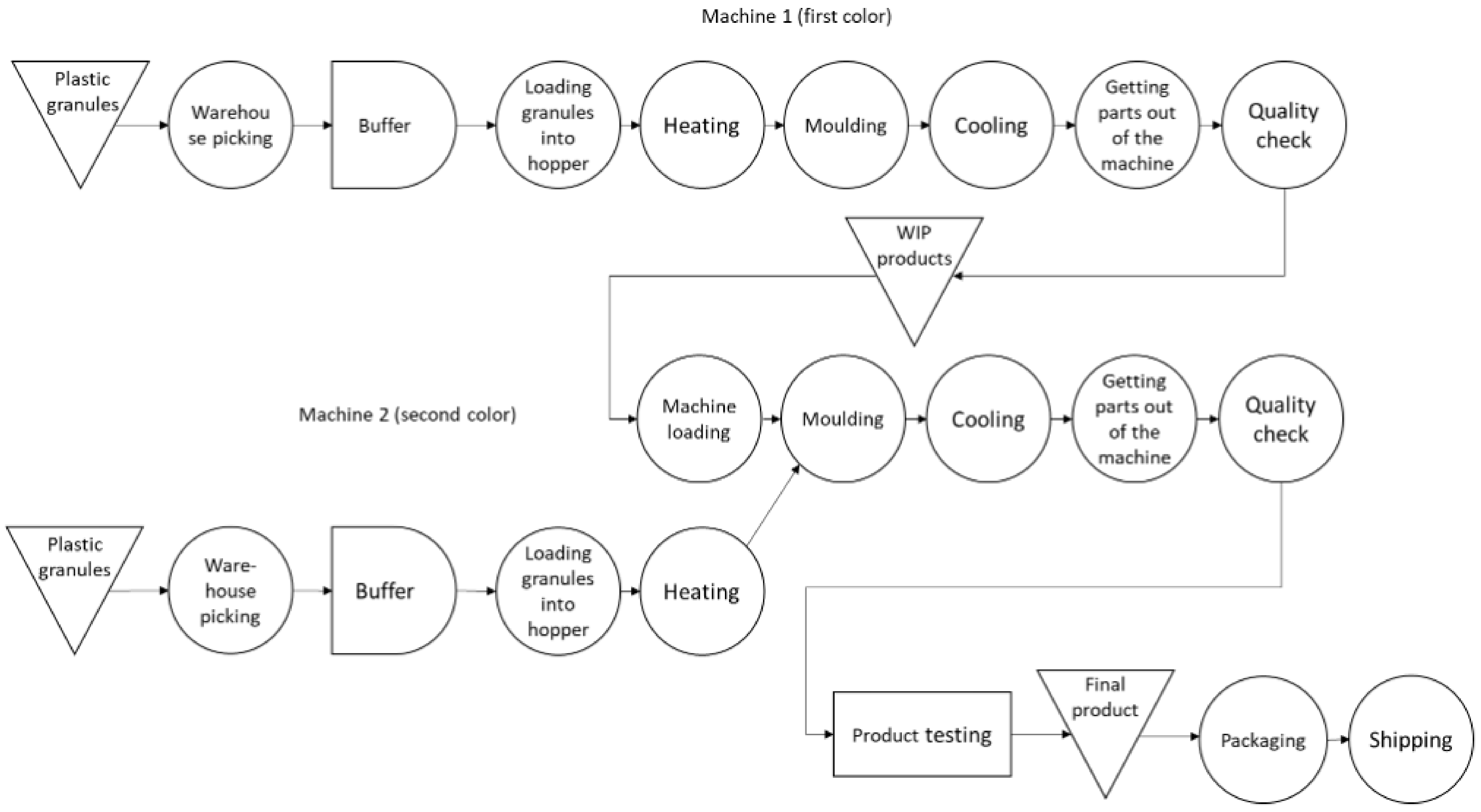
Figure 1 illustrates the production flow schema for fins, which employs two specific IMMs (labeled machines 1 and 2). The first IMM is designated as the base product, which is a paddle, whereas the second IMM is responsible for the colored booties. Plastic granules are loaded into the hopper of the first IMM. Afterward, the plastic material is heated and injected into the mold cavity. The molded product and paddles are cooled using water and the duration of the cooling phase is configurable during the configuration phase. The cycle time for a single puddle is 70 s. Once the paddles are manufactured, the bootie rubber is overprinted by inserting the previously molded base parts of the fins into the molds, which are subsequently placed into the machine. The heated colored plastic is then molded to fill the mold cavities, and the cycle time per fin pair is 160 s. The fins are cooled, inspected for quality, tested, and stored before packaging and shipment.
Recently, the industrial plant entered into contracts with a utility provider to supply electricity. According to the contract terms, the plant is priced for electricity at three different rates, depending on the time of day (7–19, 19–24, and 24–7). Therefore, the industry needs to develop production schedules that consider the hourly energy consumption and related costs over time. Regarding the daily energy consumption, historical data from January to December 2021 indicate that the plant had an average daily consumption of 135.5 kWh. The data from January to March 2022 show an average daily consumption of 156.5 kWh for the entire plant. The energy consumption of machines 1 and 2, which are referenced in
Figure 1, was collected every hour, stored in a database, and presented in table format.
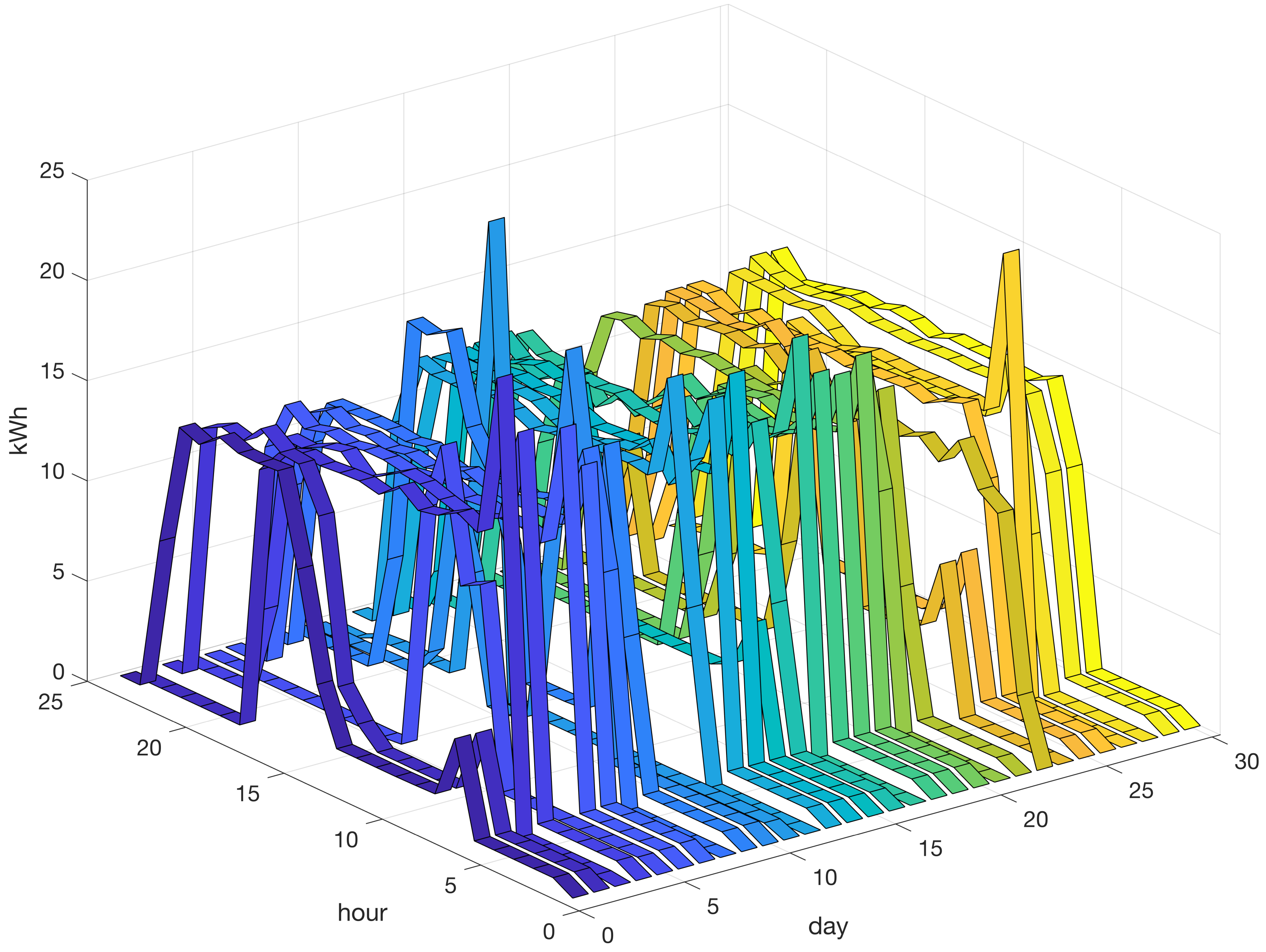
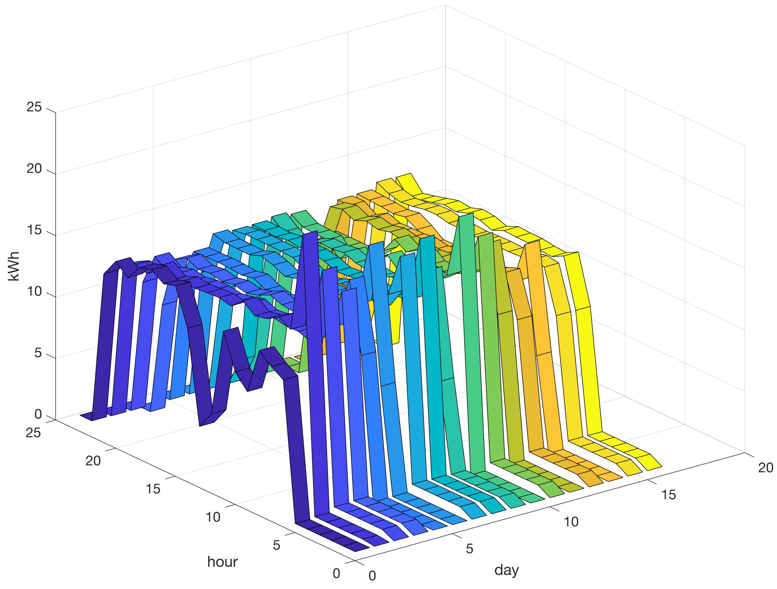
Figure 2 presents a set of 30 profiles related to the hourly energy consumption in kWh for machine 1 over 24 h. The vertical axis indicates energy consumption in kWh. Energy consumption in the dataset ranged from a minimum value close to zero to a maximum value of approximately 20 kWh. The graph indicates that during the first 5 h, the energy consumption was relatively low. From hour 6, during the first working shift of the day, the energy consumption increased to a peak and remained high during the subsequent 16 h. However, it should be noted that this pattern is not invariant because the energy consumption profile may exhibit different patterns that depend mainly on the production schedule and process parameters.
2. The Mixture Model for the Analysis of Time Series
This section presents some preliminaries regarding the methodology of mixture models for clustering. For a comprehensive discussion, refer to Fraley and Raftery [
15]. A sample is given of
n observed time series
, where
is the response (e.g., energy consumption) for the
ith individual time series given the time (predictor)
t. The time series of the index
is observed at the time values
with
. Notably,
may change from one time series to another.
A mixture model for a time series assumes that pairs
are obtained from
probability density components. A discrete random variable
indicates the component from which the pair
is drawn. The following parametric density function describes a general mixture model:
where the coefficients
are defined by
and represent the mixing probabilities such that
for each
k and
. Additionally,
(
) is the vector of the parameters for the
kth component density
, which can be chosen to represent the time series for each group
k. In our approach, the component density is a normal regression mixture [
20] and can include spline and polynomial regression [
21] and B-spline as a special case [
22].
The advantages to using spline and polynomial regression in time-series clustering include:
Smoothing: These techniques can help smooth data and reduce noise, which can be particularly useful when dealing with datasets that contain outliers.
Robustness: Spline and polynomial regression are robust to missing data and differences in sampling times between time-series data.
Ease of interpretation: The use of spline and polynomial regression can make it easier to interpret the results of the regression analysis.
Prediction: These techniques can be useful for predictions, particularly when dealing with nonlinear relationships.
Computational efficiency: Spline and polynomial regression can be computationally efficient, particularly when dealing with large datasets.
Spline regression is a highly suitable and adaptable form of regression characterized by its ability to account for nonlinear relationships between variables. This technique is commonly employed when the dataset contains outliers or when the relationship between variables cannot be accurately represented by a linear equation. In contrast, polynomial regression is a more inflexible form of regression used to model higher-order polynomial relationships between variables. This method is typically employed when the data have a well-defined and predictable relationship that can be accurately modeled by a higher-degree polynomial.
3. Regression Mixtures for Clustering Time Series with Auto-Correlated Data
For each cluster of index k, let denote an -correlation matrix. Let represent a vector of p correlation factors that ranges between and 1, and let be the standard deviation of autocorrelated noise.
The parameter vector
comprises the vector
of
r regression coefficients, noise variance
, and correlation factors of lags
. The
matrix of the regressors is denoted by
. The regression mixture is formulated using the conditional mixture density function as follows:
The vector of parameters was assessed using the expectation-maximization (EM) algorithm presented by Chamroukhi [
23]. The estimation process iteratively maximizes the following log-likelihood function:
In the E-step of the EM algorithm, starting from an initial solution
, we calculate the expected log-likelihood using the current model and data. This is performed by considering the observed time-series data and the current parameter vector
and is expressed mathematically as a formula that involves the
Q-function defined as follows:
which requires computing the posterior probabilities of the component membership
.
In step M of the EM algorithm, the value of vector
is updated by maximizing the
Q-function in Equation (
4) with respect to the entire vector
. This is accomplished through a full iteration of the algorithm for a unique parameter subset. The algorithm presented in [
24], known as the APECM, employs a disjoint partition
for each component of the index
. The algorithm implements each M step of the EM algorithm through several conditional maximization (CM) steps, during which each parameter is individually maximized based on the remaining parameters. Finally, likelihood calculations are performed for all of the time series of index
i. As noted in [
24,
25], the APECM algorithm presents a noteworthy reduction in computing costs in several respects.
The task of determining the number of clusters K involves striking a balance between the flexibility of the model and the risk of overfitting, using a criterion that evaluates this balance. To this end, an overall score function incorporating the two components was used. The first component measures the adequacy of the model in fitting the data and is typically represented by the log-likelihood . The second component measures the complexity of the model and is often expressed as the number of free parameters .
The Bayesian information criterion (BIC) and Akaike information criterion (AIC) are widely used criteria for model selection, with BIC defined as the penalized log-likelihood given by
and AIC expressed as
. These criteria are commonly employed in the statistical community and are based on the log-likelihood of the model and degrees of freedom associated with the sample size [
26,
27].
The implementation of regression mixtures is based on the hypothesis of the underlying probabilistic mixture model, in which the parameters are estimated using a sampling technique. Current research on hypothesis testing for mixture models has led to the development of various statistical methods, including the expectation-maximization (EM) test for testing homogeneity in normal mixture models [
28]. Recently, a study proposed a simple class of hypothesis test procedures for finite mixture models based on the goodness of fit (GOF) test [
29]. However, GOF test statistics do not have asymptotic limiting distributions, necessitating the development of a bootstrap procedure to approximate their distributions.
In this study, a statistical hypothesis test was not conducted due to the complexity of this approach. Instead, the suitability of the mixture models was assessed through a comparison of BIC values and the visualization of each model’s cluster centroid profile. This straightforward approach is particularly well suited for industrial engineering practitioners with limited statistical expertise, as it is accessible and easily understandable.
4. Case Study
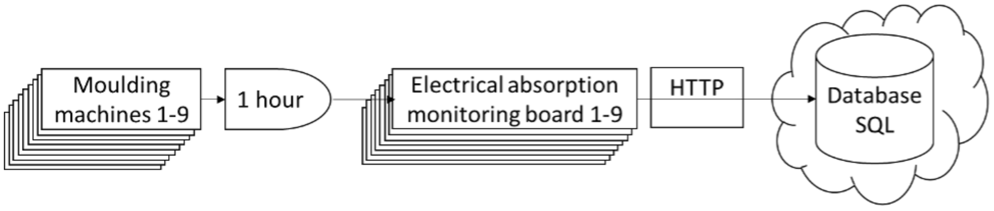
In this study, we obtained real data from the plastic industry, including the manufacture of scuba gear, freediving equipment, snorkeling devices, spearfishing equipment, and swimming accessories. The plastic components and products were fabricated using IMMs and utilized for the final product assembly. We considered nine IMMs that operate solely on electric power and can be remotely controlled to produce plastic products, such as fins, masks, and thermoplastic components. Each IMM was equipped with an electrical absorption monitoring board that recorded the energy consumption every hour and transmitted the measured values to a structured query language (SQL) database, as shown in
Figure 3.
From the SQL database, we collected a dataset comprising 119 daily time-series data points from 1 January to 30 April 2023. Each time series in the dataset pertains to the 24 h consumption of kWh for IMM no. 1. The time series exhibited various characteristics influenced by the specific production schedule of the IMM for each day. Some days may experience the IMM being idle or under maintenance, resulting in reduced consumption levels compared to periods when it is operational for production. The energy profile varies according to the current IMM production schedule.
Our research aims to establish virtual energy profiles for each cluster by grouping the hourly energy consumption patterns of each IMM in the plant. These profiles can subsequently be utilized for the accurate forecasting of energy consumption, even when changes occur in the time step (e.g., from every hour to every minute). This information is critical for effective demand-side management, resource planning, and capital budgeting. To achieve this, mixture model algorithms, such as B-spline and polynomial regression-based autocorrelated time-series clustering, have been proposed and applied to extract temporal components and classify daily load curves into distinct clusters based on their consumption patterns.
Our study employed clustering algorithms coded in MATLAB R2023a on a computing device equipped with 16 GB of memory and a 2.6 GHz Intel Core i7 processor. The clustering algorithms implemented in this study converged within a few iterations and required less than 300 s for the complete series data of four-month hourly consumption data.
4.1. The Benchmark K-Means Method for Time-Series Clustering
The
K-means algorithm is a widely adopted and efficient method for clustering data and possesses numerous advantages such as simplicity, speed, robustness, and the ability to address temporal resolution effects [
30]. Furthermore, its shape-preserving capabilities render it ideal for data clustering. These characteristics make it a suitable benchmark method for the approach proposed in this study, particularly given its widespread availability and numerous implementations for energy data clustering [
16]. However, its effectiveness is contingent on the assumption of spherical and equally varianced clusters, which may not be suitable for cases involving irregularly shaped clusters.
Note that the application of the
K-means algorithm to a sample of
n observed time series is based on the assumption that each time series of index
is observed at the same time values of index
. This assumption limits the scope of the approach because it may not account for time series sampled at different time indices in actual applications [
31].
A time series is represented by a generic point assigned to a group that should have high intracluster similarity (the sum of the squares within clusters, ) with the remaining points belonging to the same cluster, whereas it has low intercluster similarity (the sum of the squares between clusters, ) with the remaining points assigned to different groups. These two features are analytically expressed as and , where is the distance metric in (the Euclidean distance in this study).
The sum of the squared distances between each data point and its corresponding closed centroid, denoted by , is known as the within-cluster variance, . The closed centroid, , is the barycenter of the k-th cluster, , and is calculated as the average of all the data points in the cluster, , divided by the number of data points in the cluster, . The between-cluster variance is the sum of the squared distances between the mean positions of all centroids and the closed centroid . The between-cluster variance, , represents the spread of data points across all clusters.
The K-means algorithm aims to identify the cluster centers that minimize the SSW within clusters and maximize the SSB between clusters. To achieve this goal, the algorithm comprises two fundamental steps: (i) the uniform initialization of K centroids among the points to be classified and (ii) the subsequent aggregation of points around the centroids based on the distance criterion of similarity. The centroid is determined by averaging the points in each cluster, and this procedure is repeated for each cluster. The clusters and their respective centroids are then recalculated, and the process continues until the positions of the centroids exhibit minimal fluctuations, which is accomplished through the repetitive implementation of the previously mentioned steps.
4.2. The Benchmark Spectral Clustering Method for Time-Series Clustering
Unlike the
K-means algorithm, which works directly on data points, spectral clustering (SC) uses the eigenvalues and eigenvectors of a similarity matrix to group similar data points into clusters [
32,
33].
The similarity matrix is a positive semi-definite matrix , where each entry represents the affinity between data points and . A typical SC algorithm initiates with a graph , with as the set of vertices and as the weight of the edge that connects and . The objective of the SC algorithm is to identify the partition of a graph whose edge weights have low values and are contiguous. The connections between the internal vertices are associated with high-similarity indices, and graph partitioning is performed by assigning large edge weights to each cluster and small edge weights to each cluster. Mathematically, this is the problem of finding eigenvectors of the graph Laplacian from the affinity matrix and then clustering the eigenvectors into clusters.
The following steps were included in the implementation of the SC algorithm [
34]:
A similarity matrix is constructed to quantify the similarity between each pair of data points.
The eigenvalues and eigenvectors of the similarity matrix are determined.
A threshold value is established for the eigenvalue gap to separate data points into distinct clusters.
Each data point is assigned to a cluster corresponding to its eigenvector.
The SC algorithm has several advantages over the
K-means algorithm, including the ability to handle noisy data and data with nonspherical clusters, as well as the ability to visualize high-dimensional data in a lower-dimensional space. However, it is sensitive to the choice of the distance metric and similarity threshold, and there is no objective method for selecting the best threshold. In addition, it is computationally expensive, particularly for extensive datasets. Recent studies have focused on improving the scalability and robustness of spectral clustering for extremely large-scale datasets [
35].
4.3. Application of the Benchmark Algorithms to Case Study
In our research, the Caliński–Harabasz () and Davies–Bouldin () indices were employed as validation measures to determine the optimal number of clusters (K) through the K-means and SC algorithms.
The
index estimates cluster validity by calculating the ratio of the between- and within-cluster variances. This index is defined as follows [
36]:
where
n is the total number of time series and
K is the number of clusters chosen in the classification.
and
represent inter- and intracluster dispersions, respectively. A greater
index indicates better clustering results.
The
index, developed by [
37], is calculated using the mean distance between the cluster elements and their respective centroids, denoted by
, and the distance between centroids, denoted by
. The
index is expressed mathematically by the following equation, where
K represents the number of clusters, and it is desirable to minimize the
parameter according to both compactness and separation criteria.
The values of the
and
indices for the
K-means algorithm in this case study are presented in
Table 1. Based on the values in
Table 1, it can be concluded that the optimal number of clusters
K that produces the maximum value of the
index and the minimum value of the
index is equal to
. A visual illustration of the centroids for the two clusters obtained through the
K-means algorithm with
is shown in
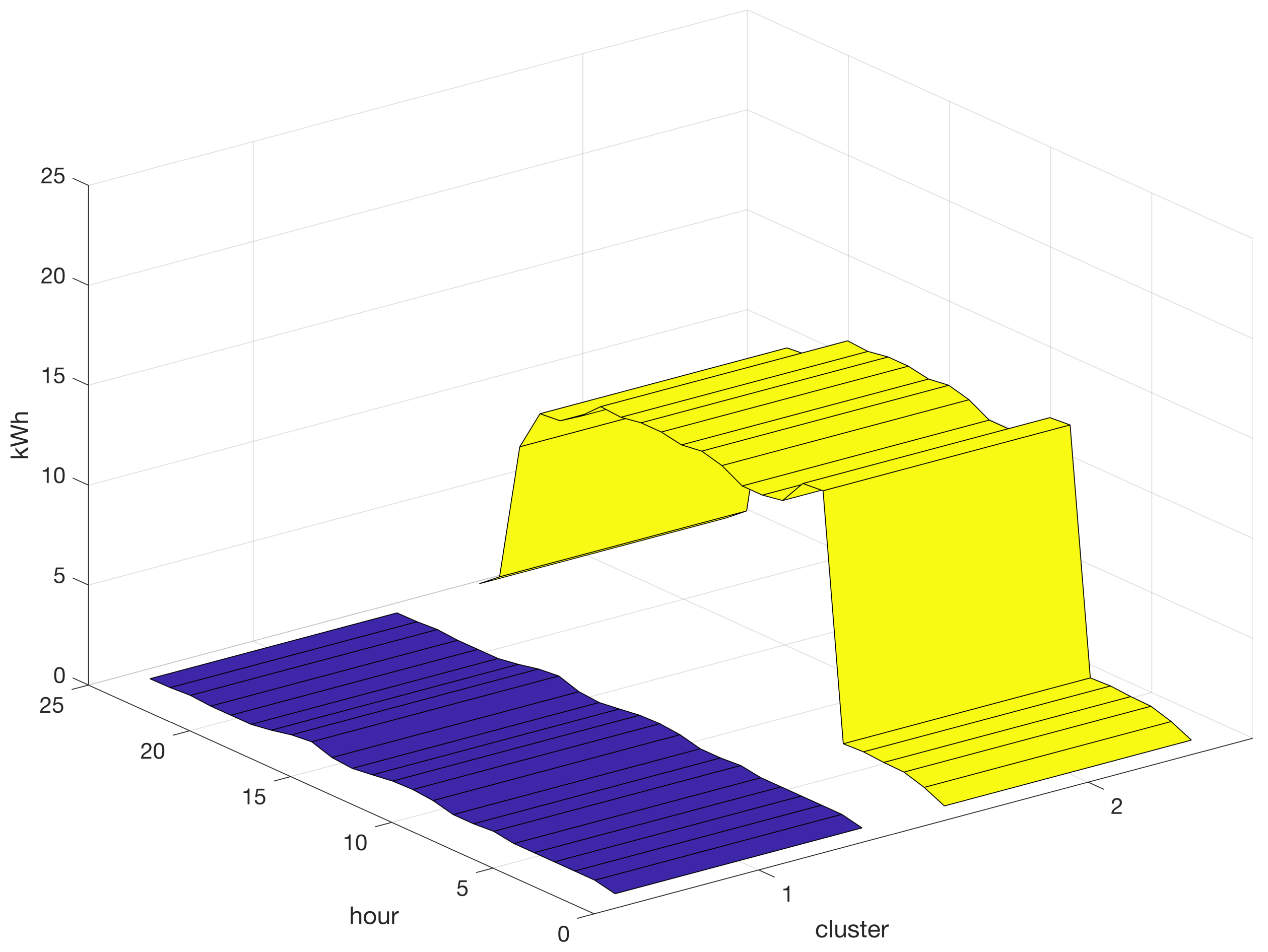
Figure 4.
Based on the results presented in
Figure 4, it can be deduced that the implementation of the
K-means algorithm in the reference case study for data mining of the energy-consumption time series is flawed in its ability to produce effective clustering. The algorithm appeared to be capable of distinguishing only between high- and low-energy load profiles. Although the
K-means algorithm is commendable for its simplicity, speed, and capacity to provide quick results, its suitability for clustering time-series data may be limited because of the nonspherical and heterogeneous nature of the energy consumption clusters in the present case study.
The values of the
and
indices for the SC algorithm in this case study are listed in
Table 2. Based on the values in
Table 2, it can be concluded that the optimal number of clusters
K that produces the maximum value of the
index and minimum value of the
index is equal to
. A graphical representation of the centroids for the three clusters generated through the implementation of the SC algorithm with
is presented in
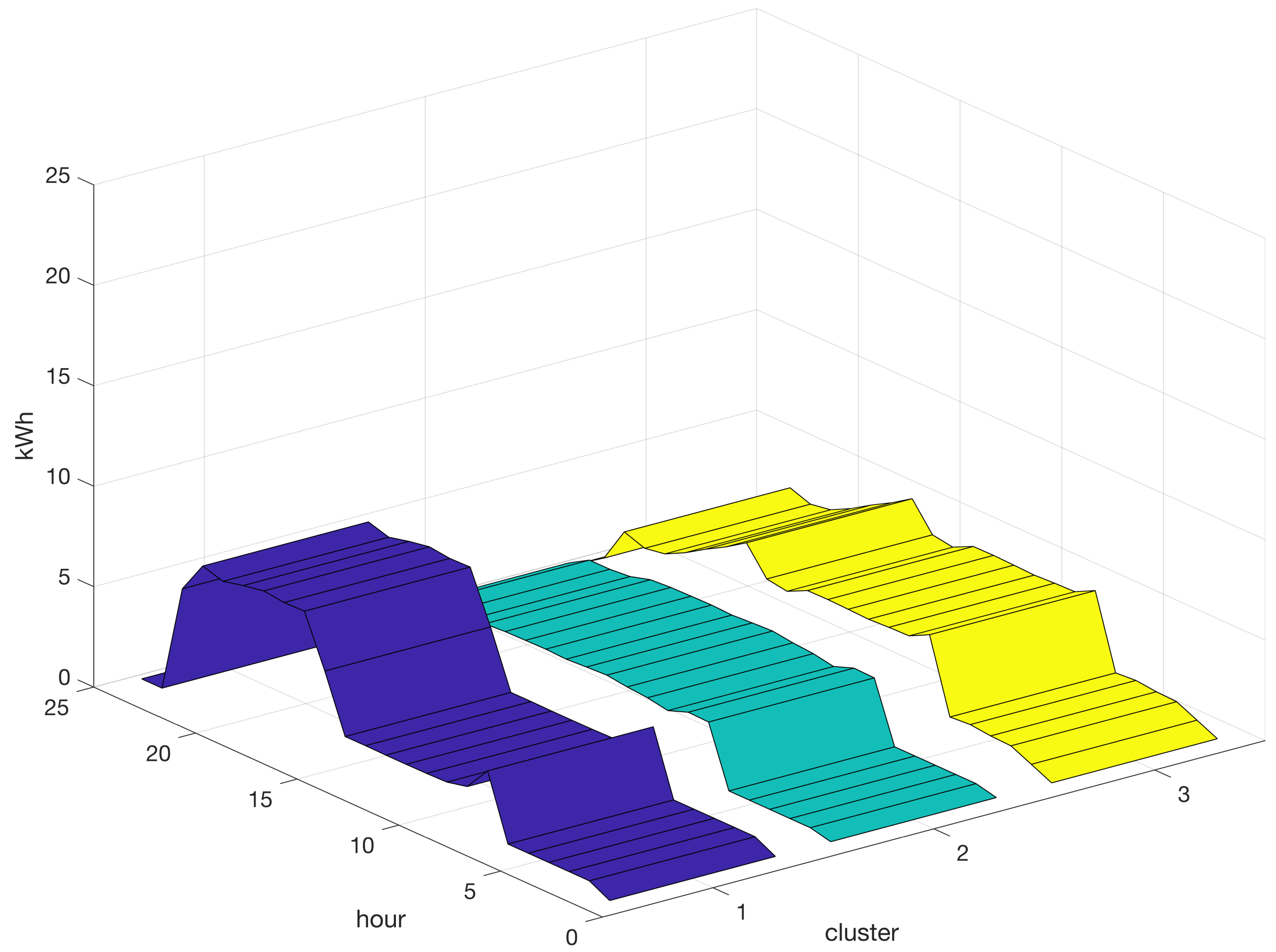
Figure 5.
Based on the findings presented in
Figure 5, it can be concluded that the implementation of the SC algorithm in the reference case study for energy consumption data mining cannot form effective clusters. Nevertheless, the SC algorithm is capable of recognizing diverse patterns of energy consumption and provides more insight than the
K-means algorithm.
4.4. B-Spline Regression Mixtures for Time-Series Clustering
An alternative algorithm for time-series clustering is regression mixtures, which overcomes the limitations of the
K-means and SC algorithms by utilizing an inference technique based on iteratively maximizing posterior probability.
Table 3 displays the BIC values obtained by fitting the B-spline regression mixtures using time-series clustering for various values of
K (ranging from one to eight) and different B-spline orders (from two to five). Our implementation employed spline knots that were uniformly distributed across the time-series domain.
The maximum BIC value, which was equal to
, was obtained when a B-spline of order three and a value of
(number of clusters) were used, as indicated in
Table 3. The log-likelihood in Equation (
3) can be maximized using the APECM algorithm. Following the implementation of the APECM algorithm, a soft partition of the time-series data into
clusters is obtained using the estimated posterior probabilities of component membership
in Equation (
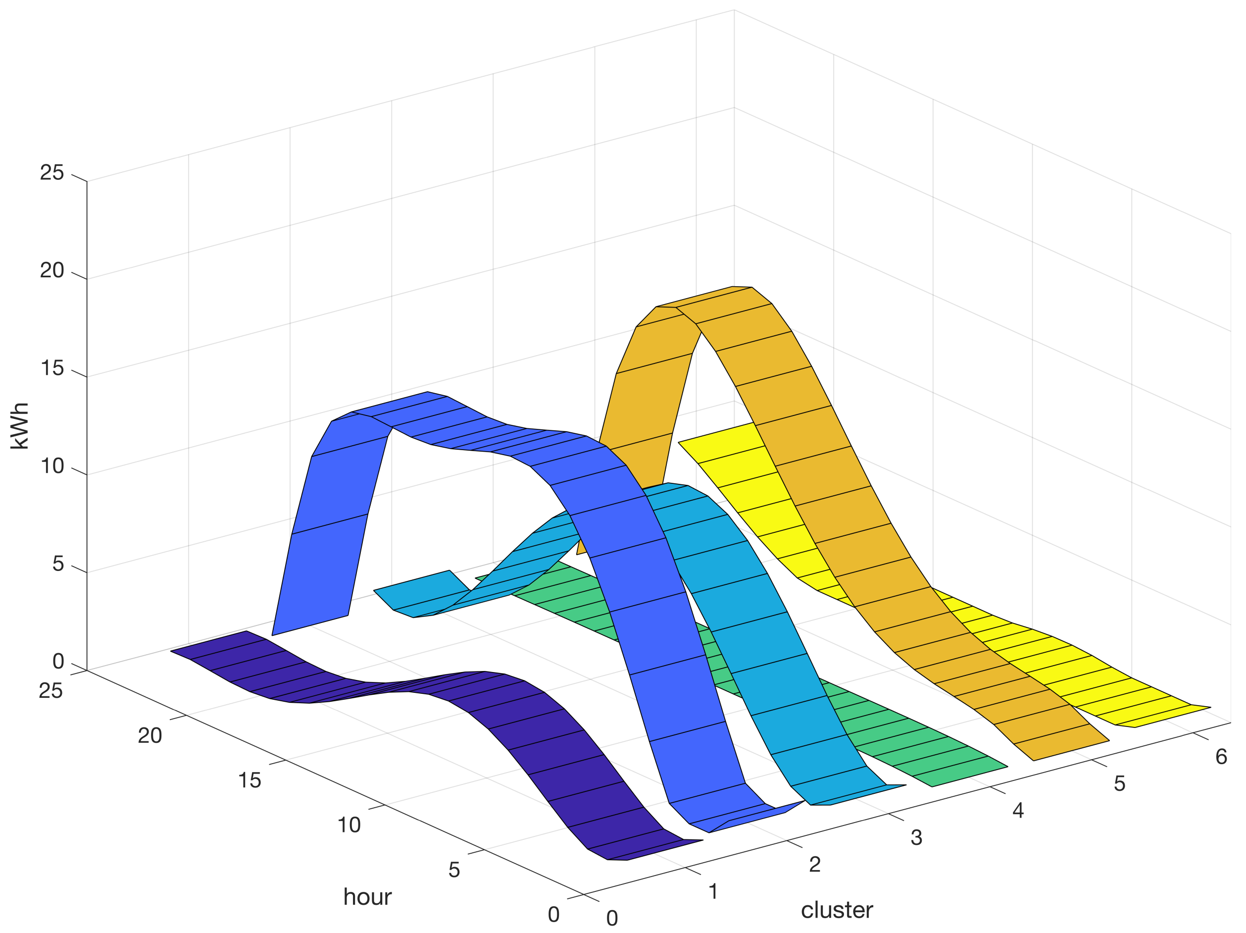
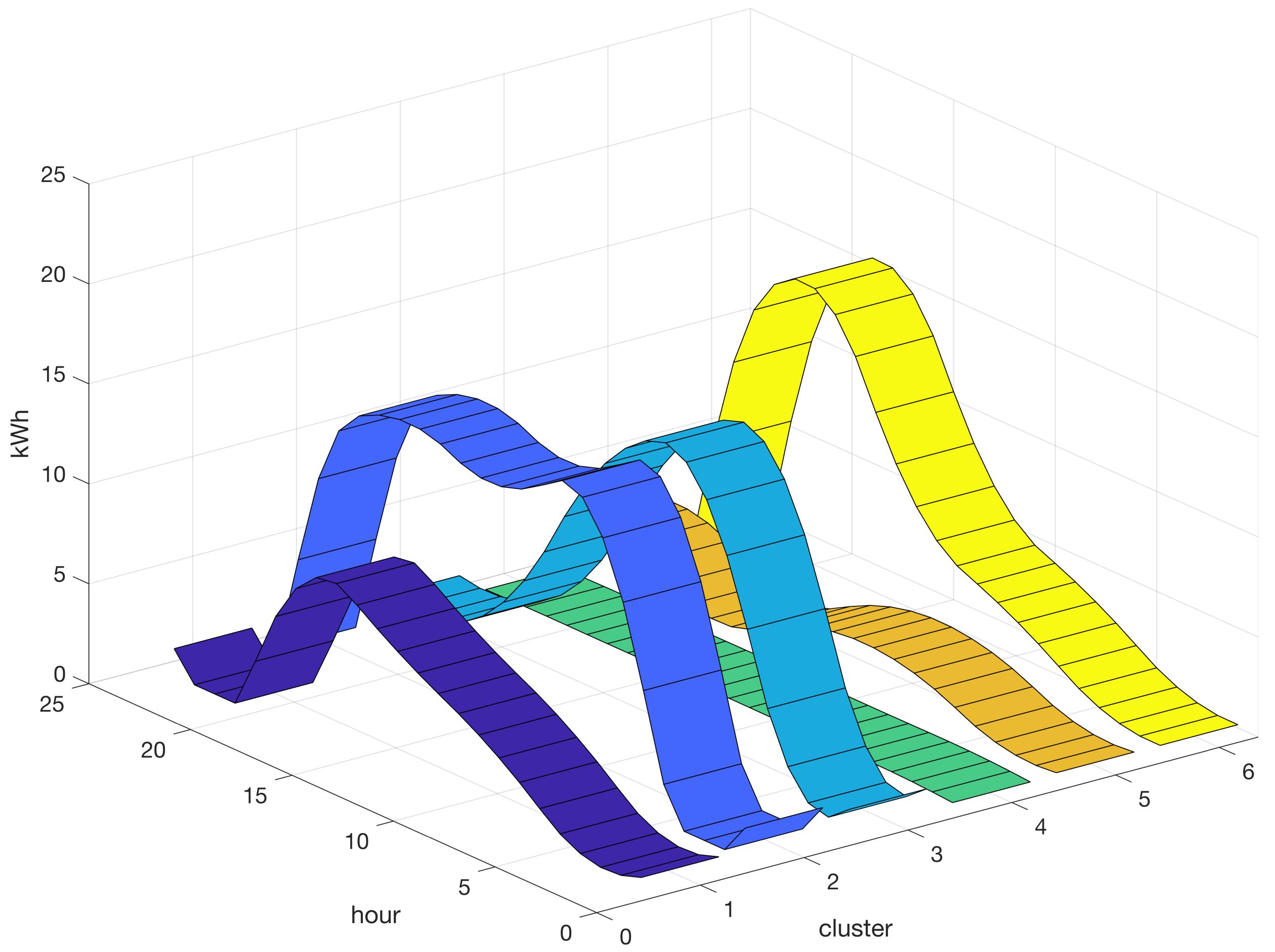
4). A hard partition can be obtained by allocating each time series to the component (cluster) with the highest posterior probability value. A graphical representation of the resulting centroids for the B-spline model of order three for each of the six clusters is shown in
Figure 6.
Figure 6 shows that B-spline regression mixtures provide valuable information for data mining. Specifically, three clusters with different shapes were identified to represent the low-load energy profiles (peaks of less than or equal to 10 kWh). Clusters 1, 4, and 5 encompassed the low-load profiles. Conversely, Clusters 2, 3, and 6 represent high-load energy profiles (peaks greater than 10 kWh and up to 15 kWh). Cluster 2 describes a high-load profile at an interval of approximately 16 h, while Clusters 3 and 6 describe high-load profiles with a shorter duration of approximately 7 h. Furthermore, Cluster 3 grouped energy profiles with high loads during the first half of the day, whereas Cluster 6 grouped energy profiles with high loads during the second half of the day. This information is of utmost importance for energy planning and consumption.
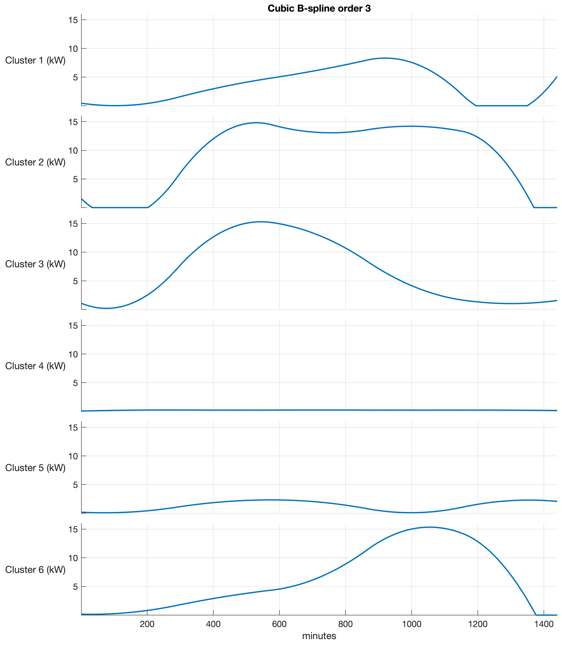
In the
K-means and SC algorithms, the centroids of each cluster have the same dimensions as points
(i.e.,
). In contrast, the centroids of the regression mixtures for time-series clustering can have dimensions of
, where
d is an upscaling or downscaling factor. For example, the centroids of the regression mixtures for time-series clustering can be represented as energy profiles with a time step of a minute, instead of an hour (
), as shown in
Figure 7.
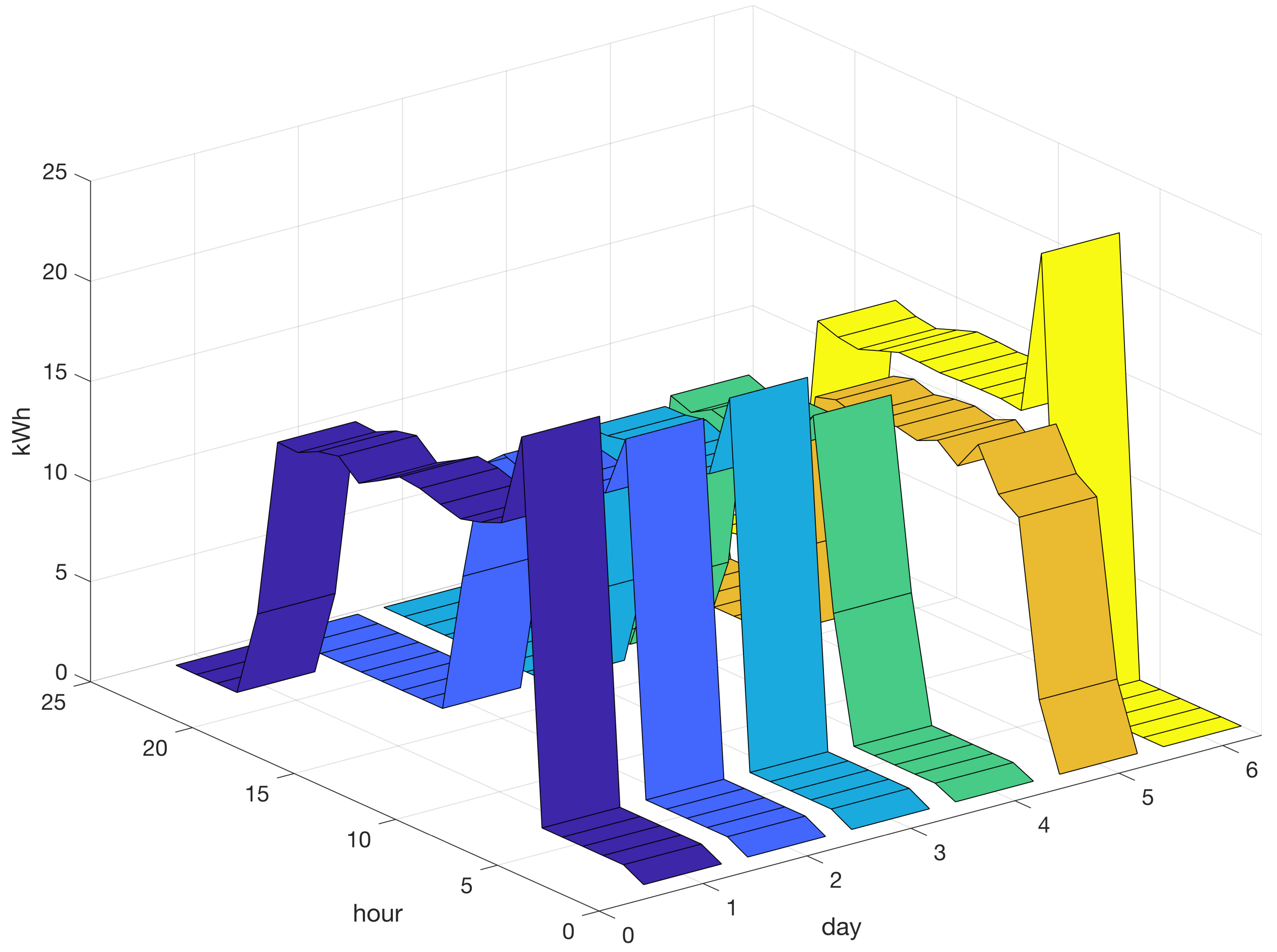
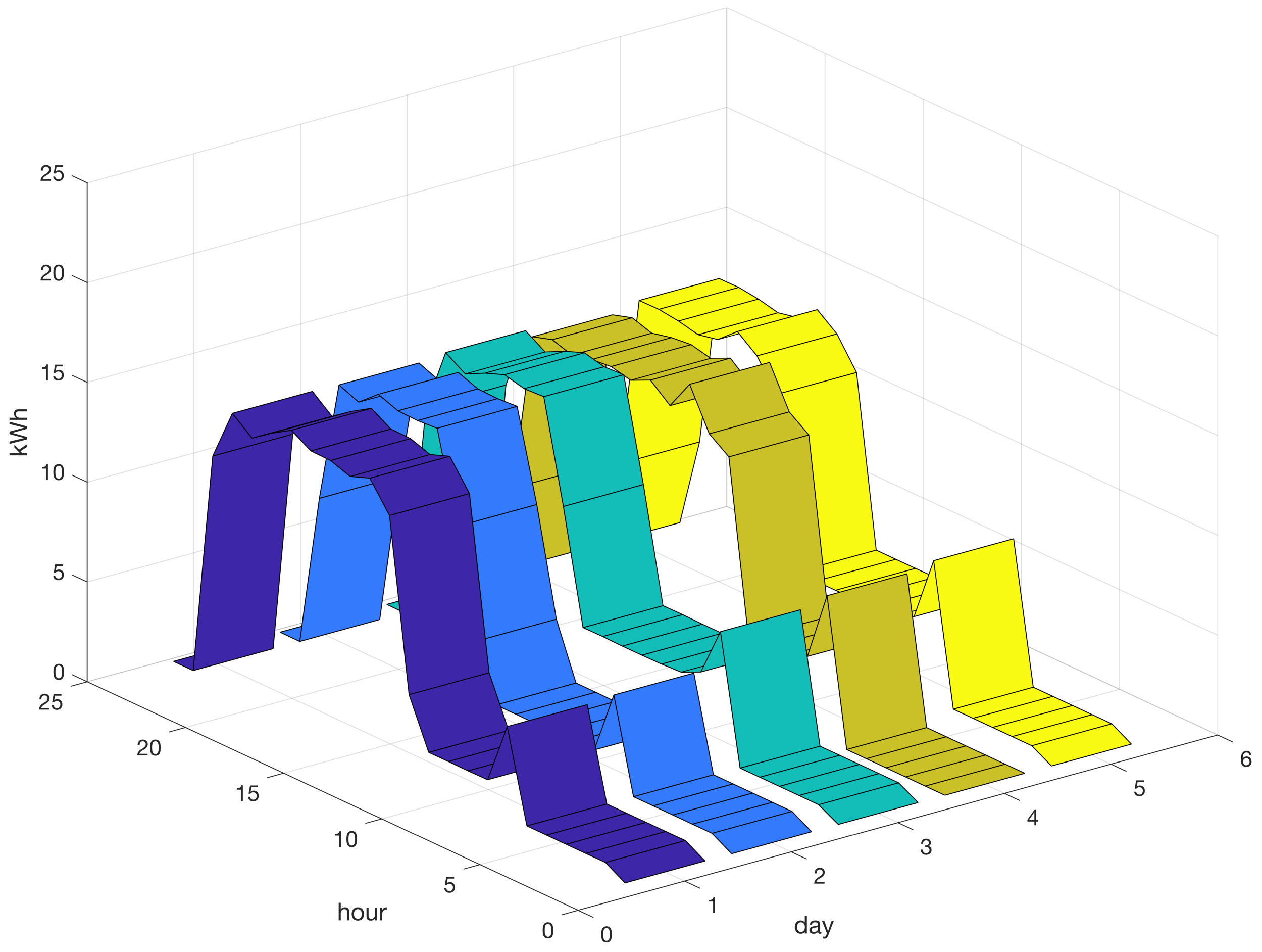
Figure 8 shows a collection of energy profiles classified as Cluster 2 (a high-load profile recurring every 16 h), whereas
Figure 9 shows a group of energy profiles grouped as Cluster 3 (a high-load profile lasting for 7 h during the first half of the day).
Figure 10 illustrates a set of energy profiles classified as Cluster 6 (a high-load profile lasting seven hours in the second half of the day).
4.5. Polynomial Regression Mixtures for Time-Series Clustering
Polynomial regression is an alternative to B-spline regression for time-series clustering. The resulting fourth-order polynomial models are shown in
Figure 11.
Analysis of these clusters revealed distinct shapes and corresponding load profiles. Six clusters were identified, with Clusters 1, 4, and 6 exhibiting low-load energy profiles and Clusters 2, 3, and 5 displaying high-load energy profiles. Notably, Cluster 2 demonstrated a high-load profile at an interval of approximately 16 h, whereas Clusters 3 and 6 revealed high-load profiles with a shorter duration. Cluster 3 grouped energy profiles with a high load during the first half of the day, whereas Cluster 6 grouped energy profiles with a high load during the second half of the day. These findings are consistent with those previously discussed for B-spline regression.
5. Conclusions
This study delineates a method and associated algorithms for tracking the energy consumption in injection molding operations, which are the most energy-intensive processes in the plastics industry. The energy profiles collected from a real industrial plant were analyzed using data mining algorithms to identify distinct clusters that represent the specific energy consumption profiles of various production variants.
We utilized mixtures of regression models due to their flexibility in modeling heterogeneous time series and clustering time series in an unsupervised machine-learning framework. We opted to analyze the mixture models because of their robust statistical foundation and the interpretability of their results. Furthermore, because clusters correspond to the model components, the number of clusters can be easily determined by utilizing the likelihood function for the components in the mixture model.
Mixture regression models assume that observations are independent and identically distributed, which may not be true for time-series data. Additionally, the model assumes that the errors are normally distributed, which may not be the case for the energy consumption data. Therefore, we developed a method for clustering autocorrelated time-series data that combines the APECM algorithm with B-spline and polynomial regressions within a mixture regression framework. This approach has been shown to outperform popular techniques such as the K-means and SC algorithms through its application to real-world data. Our analysis led to the accurate grouping of the energy consumption profiles, where each cluster was associated with a specific production schedule. The clustering method also provides a unique profile of energy consumption for each cluster depending on the production schedule and regression approach. Through these profiles, we identified information related to the shape of energy consumption, which provided insights into reducing the electrical demand of the plant.
Our research presents a parametric model-based approach that provides a precise representation of energy consumption profiles. This method is particularly well suited for practical industrial applications, as it is an automated, data-driven approach within an unsupervised training framework. The selection of an appropriate model structure, including the types and orders of the regressors and the number of clusters, is a critical task that must be performed by the analyst. To address this challenge, we employed a BIC-based rule for model selection.
The primary limitation of the mixture regression models presented in this study is their vulnerability to overfitting, particularly when the number of components is large or when the data are noisy. Overfitting can result in poor generalization performance and inaccurate cluster labels. In future work, we will focus on implementing techniques to mitigate overfitting in mixture regression models for clustering time-series data. These techniques may include the application of regularization methods, such as
or
regularization [
38], and feature selection methods, such as backward elimination or LASSO [
39]. Additionally, shrinkage methods, such as ridge regression, may be employed to penalize the coefficients and reduce overfitting [
40].
Further work in this area includes the incorporation of additional variables into the mixture models to assess their impact on the clustering performance and the exploration of supervised learning techniques, such as support vector machines (SVMs) or neural networks, to determine their potential to improve the accuracy of clustering.
Author Contributions
Conceptualization, M.P.; methodology, M.P.; software, M.P.; validation, M.P. and G.P.; resources, M.M. and G.P.; writing—original draft preparation, M.P.; writing—review and editing, M.P. and M.M.; supervision, M.M. and G.P.; project administration, M.M.; funding acquisition, G.P. All authors have read and agreed to the published version of the manuscript.
Funding
This work has been funded by Puglia Region (Italy)—Project TANDEM ‘digiTAl twiN green aDvancEd Manufacturing’ (P.O. PUGLIA FESR 2014-2020).
Data Availability Statement
The data used to support the findings of this study can be obtained from the corresponding author upon reasonable request.
Acknowledgments
The authors express their appreciation to the SEACSUB industry in San Colombano Certenoli (GE, Italy) for providing the data used in the case study. Additionally, the STAM S.r.l. industry in Genova (Italy) is acknowledged for its significant contribution to the dataset collection.
Conflicts of Interest
Author M.M. was employed by the company DGS S.p.A, Italy. The remaining authors declare that the research was conducted in the absence of any commercial or financial relationships that could be construed as a potential conflict of interest. The funder had no role in the design of this study; in the collection, analyses, or interpretation of data; in the writing of the manuscript; nor in the decision to publish the results.
References
- Elduque, A.; Elduque, D.; Javierre, C.; Fernández, Á.; Santolaria, J. Environmental impact analysis of the injection molding process: Analysis of the processing of high-density polyethylene parts. J. Clean. Prod. 2015, 108, 80–89. [Google Scholar] [CrossRef]
- Kazmer, D.; Peterson, A.M.; Masato, D.; Colon, A.R.; Krantz, J. Strategic cost and sustainability analyses of injection molding and material extrusion additive manufacturing. Polym. Eng. Sci. 2023, 63, 943–958. [Google Scholar] [CrossRef]
- Dunkelberg, H.; Schlosser, F.; Veitengruber, F.; Meschede, H.; Heidrich, T. Classification and clustering of the German plastic industry with a special focus on the implementation of low and high temperature waste heat. J. Clean. Prod. 2019, 238, 117784. [Google Scholar] [CrossRef]
- Rashid, O.; Low, K.; Pittman, J. Mold cooling in thermoplastics injection molding: Effectiveness and energy efficiency. J. Clean. Prod. 2020, 264, 121375. [Google Scholar] [CrossRef]
- Kelly, A.; Woodhead, M.; Coates, P. Comparison of injection molding machine performance. Polym. Eng. Sci. 2005, 45, 857–865. [Google Scholar] [CrossRef]
- Liu, H.; Zhang, X.; Quan, L.; Zhang, H. Research on energy consumption of injection molding machine driven by five different types of electro-hydraulic power units. J. Clean. Prod. 2020, 242, 118355. [Google Scholar] [CrossRef]
- Elduque, A.; Elduque, D.; Pina, C.; Clavería, I.; Javierre, C. Electricity consumption estimation of the polymer material injection-molding manufacturing process: Empirical model and application. Materials 2018, 11, 1740. [Google Scholar] [CrossRef]
- Meekers, I.; Refalo, P.; Rochman, A. Analysis of process parameters affecting energy consumption in plastic injection moulding. Procedia CIRP 2018, 69, 342–347. [Google Scholar] [CrossRef]
- Ishihara, M.; Hibino, H.; Harada, T. Simulated annealing based simulation method for minimizing electricity cost considering production line scheduling including injection molding machines. J. Adv. Mech. Des. Syst. Manuf. 2020, 14, JAMDSM0055. [Google Scholar] [CrossRef]
- Wu, Y.; Feng, Y.; Peng, S.; Mao, Z.; Chen, B. Generative machine learning-based multi-objective process parameter optimization towards energy and quality of injection molding. Environ. Sci. Pollut. Res. 2023, 30, 51518–51530. [Google Scholar] [CrossRef]
- Mianehrow, H.; Abbasian, A. Energy monitoring of plastic injection molding process running with hydraulic injection molding machines. J. Clean. Prod. 2017, 148, 804–810. [Google Scholar] [CrossRef]
- Ahir, R.K.; Chakraborty, B. A novel cluster-specific analysis framework for demand-side management and net metering using smart meter data. Sustain. Energy Grids Netw. 2022, 31, 100771. [Google Scholar] [CrossRef]
- Aghabozorgi, S.; Shirkhorshidi, A.S.; Wah, T.Y. Time-series clustering—A decade review. Inf. Syst. 2015, 53, 16–38. [Google Scholar] [CrossRef]
- Javed, A.; Lee, B.S.; Rizzo, D.M. A benchmark study on time series clustering. Mach. Learn. Appl. 2020, 1, 100001. [Google Scholar] [CrossRef]
- Fraley, C.; Raftery, A.E. Model-based clustering, discriminant analysis, and density estimation. J. Am. Stat. Assoc. 2002, 97, 611–631. [Google Scholar] [CrossRef]
- Okereke, G.E.; Bali, M.C.; Okwueze, C.N.; Ukekwe, E.C.; Echezona, S.C.; Ugwu, C.I. K-means clustering of electricity consumers using time-domain features from smart meter data. J. Electr. Syst. Inf. Technol. 2023, 10, 1–18. [Google Scholar] [CrossRef]
- Zheng, P.; Zhou, H.; Liu, J.; Nakanishi, Y. Interpretable building energy consumption forecasting using spectral clustering algorithm and temporal fusion transformers architecture. Appl. Energy 2023, 349, 121607. [Google Scholar] [CrossRef]
- Pacella, M.; Papadia, G. Finite Mixture Models for Clustering Auto-Correlated Sales Series Data Influenced by Promotions. Computation 2022, 10, 23. [Google Scholar] [CrossRef]
- Czepiel, M.; Bańkosz, M.; Sobczak-Kupiec, A. Advanced Injection Molding Methods. Materials 2023, 16, 5802. [Google Scholar] [CrossRef] [PubMed]
- Gaffney, S.; Smyth, P. Curve Clustering with Random Effects Regression Mixtures. In Proceedings of the Ninth International Workshop on Artificial Intelligence and Statistics, Key West, FL, USA, 3–6 January 2003; Bishop, C.M., Frey, B.J., Eds.; Machine Learning Research. JMLR: Cambridge, MA, USA, 2003; Volume R4, pp. 101–108. [Google Scholar]
- James, G.M.; Sugar, C.A. Clustering for Sparsely Sampled Functional Data. J. Am. Stat. Assoc. 2003, 98, 397–408. [Google Scholar] [CrossRef]
- Liu, X.; Yang, M.C. Simultaneous curve registration and clustering for functional data. Comput. Stat. Data Anal. 2009, 53, 1361–1376. [Google Scholar] [CrossRef]
- Chamroukhi, F. Unsupervised learning of regression mixture models with unknown number of components. J. Stat. Comput. Simul. 2016, 86, 2308–2334. [Google Scholar] [CrossRef]
- Chen, W.C.; Maitra, R. Model-based clustering of regression time series data via APECM—an AECM algorithm sung to an even faster beat. Stat. Anal. Data Mining ASA Data Sci. J. 2011, 4, 567–578. [Google Scholar] [CrossRef]
- Chen, W.C.; Ostrouchov, G.; Pugmire, D.; Prabhat; Wehner, M. A parallel EM algorithm for model-based clustering applied to the exploration of large spatio-temporal data. Technometrics 2013, 55, 513–523. [Google Scholar] [CrossRef]
- Schwarz, G. Estimating the Dimension of a Model. Ann. Stat. 1978, 6, 461–464. [Google Scholar] [CrossRef]
- Akaike, H. A new look at the statistical model identification. IEEE Trans. Autom. Control. 1974, 19, 716–723. [Google Scholar] [CrossRef]
- Chen, J.; Li, P. Hypothesis test for normal mixture models: The EM approach. Ann. Stat. 2009, 37, 2523–2542. [Google Scholar] [CrossRef]
- Wichitchan, S.; Yao, W.; Yang, G. Hypothesis testing for finite mixture models. Comput. Stat. Data Anal. 2019, 132, 180–189. [Google Scholar] [CrossRef]
- Ahmed, M.; Seraj, R.; Islam, S.M. The k-means algorithm: A comprehensive survey and performance evaluation. Electronics 2020, 9, 1295. [Google Scholar] [CrossRef]
- Holder, C.; Middlehurst, M.; Bagnall, A. A review and evaluation of elastic distance functions for time series clustering. Knowl. Inf. Syst. 2023, 1–45. [Google Scholar] [CrossRef]
- Jia, H.; Ding, S.; Xu, X.; Nie, R. The latest research progress on spectral clustering. Neural Comput. Appl. 2014, 24, 1477–1486. [Google Scholar] [CrossRef]
- Zhang, J.; Shen, Y. Review on spectral methods for clustering. In Proceedings of the 2015 34th Chinese Control Conference (CCC), Hangzhou, China, 28–30 July 2015; pp. 3791–3796. [Google Scholar]
- Pacella, M.; Papadia, G. Fault diagnosis by multisensor data: A data-driven approach based on spectral clustering and pairwise constraints. Sensors 2020, 20, 7065. [Google Scholar] [CrossRef] [PubMed]
- Huang, D.; Wang, C.-D.; Wu, J.-S.; Lai, J.-H.; Kwoh, C.-K. Ultra-scalable spectral clustering and ensemble clustering. IEEE Trans. Knowl. Data Eng. 2019, 32, 1212–1226. [Google Scholar] [CrossRef]
- Caliński, T.; Harabasz, J. A dendrite method for cluster analysis. Commun.-Stat.-Theory Methods 1974, 3, 1–27. [Google Scholar] [CrossRef]
- Davies, D.L.; Bouldin, D.W. A cluster separation measure. IEEE Trans. Pattern Anal. Mach. Intell. 1979, PAMI-1, 224–227. [Google Scholar] [CrossRef]
- Kolluri, J.; Kotte, V.K.; Phridviraj, M.S.B.; Razia, S. Reducing overfitting problem in machine learning using novel L1/4 regularization method. In Proceedings of the 2020 4th International Conference on Trends in Electronics and Informatics (ICOEI)(48184), Tirunelveli, India, 15–17 June 2020; pp. 934–938. [Google Scholar]
- Lloyd-Jones, L.R.; Nguyen, H.D.; McLachlan, G.J. A globally convergent algorithm for lasso-penalized mixture of linear regression models. Comput. Stat. Data Anal. 2018, 119, 19–38. [Google Scholar] [CrossRef]
- Zhang, R.; Li, X.; Wu, T.; Zhao, Y. Data clustering via uncorrelated ridge regression. IEEE Trans. Neural Netw. Learn. Syst. 2020, 32, 450–456. [Google Scholar] [CrossRef]
Figure 1.
Process flow chart for fins production. The production of fins is managed through two IIMs (machine 1 and 2). Machine 1 is used for the creation of the base product, namely paddles, while machine 2 is used for colored booties. (Image courtesy of STAM and SEACSUB).
Figure 1.
Process flow chart for fins production. The production of fins is managed through two IIMs (machine 1 and 2). Machine 1 is used for the creation of the base product, namely paddles, while machine 2 is used for colored booties. (Image courtesy of STAM and SEACSUB).
Figure 2.
Historical time-series dataset comprising 30 instances of hourly energy consumption in kilowatt-hours (kWh) on machine 1 on 24 h for 30 days. The vertical axis represents the energy consumption in kWh, and a different color is used to distinguish between the various production days in the dataset.
Figure 3.
Collection and recording of hourly energy consumption data of nine IMMs into the SQL database for effective data management and analysis.
Figure 3.
Collection and recording of hourly energy consumption data of nine IMMs into the SQL database for effective data management and analysis.
Figure 4.
Graphical representation of the centroids for the two clusters generated through the implementation of the K-means algorithm with . Varying colors differentiate profiles.
Figure 4.
Graphical representation of the centroids for the two clusters generated through the implementation of the K-means algorithm with . Varying colors differentiate profiles.
Figure 5.
Graphical representation of the centroids for the two clusters generated through the implementation of the SC algorithm with . Varying colors differentiate profiles.
Figure 5.
Graphical representation of the centroids for the two clusters generated through the implementation of the SC algorithm with . Varying colors differentiate profiles.
Figure 6.
Graphical depiction of the centroids for each of the six clusters (1–6) resulting from the implementation of B-spline regression mixtures. Varying colors differentiate profiles.
Figure 6.
Graphical depiction of the centroids for each of the six clusters (1–6) resulting from the implementation of B-spline regression mixtures. Varying colors differentiate profiles.
Figure 7.
Graphical representation of the B-spline of order 3 resulting from the EM algorithm resampled at a frequency of a minute in 24 h (1440 data points).
Figure 7.
Graphical representation of the B-spline of order 3 resulting from the EM algorithm resampled at a frequency of a minute in 24 h (1440 data points).
Figure 8.
Sixteen energy profiles grouped into Cluster 2, exhibiting a high-load profile spanning a period of approximately 16 h. Varying colors differentiate profiles.
Figure 8.
Sixteen energy profiles grouped into Cluster 2, exhibiting a high-load profile spanning a period of approximately 16 h. Varying colors differentiate profiles.
Figure 9.
Six energy profiles grouped into Cluster 3, exhibiting a high-load profile spanning a period of approximately 7 h during the first half of the day. Varying colors differentiate profiles.
Figure 9.
Six energy profiles grouped into Cluster 3, exhibiting a high-load profile spanning a period of approximately 7 h during the first half of the day. Varying colors differentiate profiles.
Figure 10.
Five energy profiles grouped into Cluster 6, exhibiting a high-load profile spanning a period of approximately 7 h during the second half of the day. Varying colors differentiate profiles.
Figure 10.
Five energy profiles grouped into Cluster 6, exhibiting a high-load profile spanning a period of approximately 7 h during the second half of the day. Varying colors differentiate profiles.
Figure 11.
Graphical depiction of the centroids for each of the six clusters (1–6) resulting from the implementation of polynomial regression mixtures. Varying colors differentiate profiles.
Figure 11.
Graphical depiction of the centroids for each of the six clusters (1–6) resulting from the implementation of polynomial regression mixtures. Varying colors differentiate profiles.
Table 1.
Values of the and indices for different values of K for the K-means algorithm in the reference case study. The maximum value of and minimum value of are obtained for .
Table 1.
Values of the and indices for different values of K for the K-means algorithm in the reference case study. The maximum value of and minimum value of are obtained for .
| | CH | DB |
|---|
| | |
| | |
| | |
| | |
| | |
| | |
| | |
| | |
Table 2.
Values of the and indices for different values of K for the SC algorithm in the reference case study. The maximum value of and minimum value of are obtained for .
Table 2.
Values of the and indices for different values of K for the SC algorithm in the reference case study. The maximum value of and minimum value of are obtained for .
| | CH | DB |
|---|
| | |
| | |
| | |
| | |
| | |
| | |
| | |
| | |
Table 3.
BIC values for B-spline regression mixtures for different values of K and orders. The maximum BIC value is obtained for and B-spline of order 3 (BIC equal to ).
Table 3.
BIC values for B-spline regression mixtures for different values of K and orders. The maximum BIC value is obtained for and B-spline of order 3 (BIC equal to ).
| | Order 2 | Order 3 | Order 4 | Order 5 |
|---|
| | | | |
| | | | |
| | | | |
| | | | |
| | | | |
| | | | |
| | | | |
| | | | |
| Disclaimer/Publisher’s Note: The statements, opinions and data contained in all publications are solely those of the individual author(s) and contributor(s) and not of MDPI and/or the editor(s). MDPI and/or the editor(s) disclaim responsibility for any injury to people or property resulting from any ideas, methods, instructions or products referred to in the content. |
© 2023 by the authors. Licensee MDPI, Basel, Switzerland. This article is an open access article distributed under the terms and conditions of the Creative Commons Attribution (CC BY) license (https://creativecommons.org/licenses/by/4.0/).


