Assessing Algorithms Used for Constructing Confidence Ellipses in Multidimensional Scaling Solutions

Abstract

This paper assesses algorithms proposed for constructing confidence ellipses in multidimensional scaling (MDS) solutions and proposes a new approach to interpreting these confidence ellipses via hierarchical cluster analysis (HCA). It is shown that the most effective algorithm for constructing confidence ellipses involves the generation of simulated distances based on the original multivariate dataset and then the creation of MDS maps that are scaled, reflected, rotated, translated, and finally superimposed. For this algorithm, the stability measure of the average areas tends to zero with increasing sample size n following the power model, An^−B, with positive B values ranging from 0.7 to 2 and high R-squared fitting values around 0.99. This algorithm was applied to create confidence ellipses in the MDS plots of squared Euclidean and Mahalanobis distances for continuous and binary data. It was found that plotting confidence ellipses in MDS plots offers a better visualization of the distance map of the populations under study compared to plotting single points. However, the confidence ellipses cannot eliminate the subjective selection of clusters in the MDS plot based simply on the proximity of the MDS points. To overcome this subjective selection, we should quantify the formation of clusters of proximal samples. Thus, in addition to the algorithm assessment, we propose a new approach that estimates all possible cluster probabilities associated with the confidence ellipses by applying HCA using distance matrices derived from these ellipses.

1. Introduction

Multidimensional scaling (MDS) comprises a set of statistical techniques for visualizing the degree of similarity of individual cases or groups in cases of a multivariate dataset [1,2,3]. The original dataset is transformed into a distance or similarity matrix, from which a map of points is produced in a low-dimensional Euclidean space. This process facilitates the detection of patterns that are not obvious from the original multivariate dataset. For this reason, the applications of MDS cover a wide range of diverse fields, such as sociology, physics, biology, anthropology, and others.

The effectiveness of MDS in exploring patterns in a multivariate dataset has two main limitations: First, selecting clusters in the MDS plot based simply on the proximity of the MDS points is a subjective process that, furthermore, does not take into account the error in the calculated distances. An improvement over this limitation is to use two-dimensional MDS plots with confidence ellipses. There are several algorithms proposed to create MDS confidence ellipses [4,5,6,7,8,9,10,11,12,13,14]. These plots do provide a better visualization of the distance map, but again, the selection of clusters in the MDS plot is subjective. Moreover, as shown in this paper, from MDS plots with confidence ellipses, we cannot confidently infer possible clusters between the samples, and false conclusions may be drawn. The second limitation concerns the application of MDS using squared Euclidean and Mahalanobis-type distances with correction for small sample sizes [15]. This group of distances is extensively used in biodistance studies to explore population divergence and population history since the correction for small sample sizes makes the Euclidean/Mahalanobis-type distances unbiased estimators of the corresponding population distances [15]. However, the correction for small sample sizes can lead to negative distance values, which makes it impossible to directly apply the MDS method.

In this paper, we address the above limitations in an attempt to provide a solution to the quantitative selection of clusters of proximal samples using MDS solutions. Thus, we first evaluate the algorithms proposed for constructing confidence ellipses in MDS solutions and identify the most efficient of them for constructing confidence ellipses when using squared Euclidean and Mahalanobis-type distances in continuous and binary multivariate datasets. Then, for the quantitative selection of clusters, we propose a new approach that estimates all possible cluster probabilities and the most probable dendrogram that is related to the confidence ellipses of the MDS, as well as the probability of obtaining this dendrogram, by applying HCA using distance matrices derived from the confidence ellipses. The case of negative distance measures is also thoroughly examined, and the most appropriate approach to solving it is determined.

2. Theoretical Background

2.1. Methods for Creating Confidence Ellipses in MDS Plots

In the relevant literature, MDS confidence ellipses are closely related to the stability of a MDS solution [4]. The stability methods for a MDS solution examined were the following:

• Pseudo-confidence ellipses (PCE). This method has been proposed by De Leeuw [5] and creates pseudo-confidence ellipses around MDS points based on an implementation of the Hessian of the stress loss function. However, the area of the pseudo-confidence ellipses depends upon the value of a parameter ε, which shows that the stress value at the perturbation region should be at most 100 ε% larger than the local minimum of the stress loss function. Thus, in fact, the calculation of confidence ellipses assumes an arbitrary choice of the value of parameter ε.
• Jackknife method (JACmds). This has been developed by De Leeuw and Meulman [6], who proposed a leave-one-out method that can be used both in metric and nonmetric MDS. The jackknife MDS plot is a graph with stars, where the centers of the stars are the jackknife centroids and the rays are the jackknife solutions. In the present study, we have added a convex hull to the points of each star, and we have calculated their areas.
• Bootstrapping of the MDS residuals (BOOTres). This method is described in the manual of the MultBiplotR package of R in the details of the BootstrapDistance function [7]. It is based on the study carried out by Ringrose [8], Efron and Tibshirani [9], and Milan and Whittaker [10] and uses random sampling or permutations of MDS residuals to obtain the bootstrap replications that are used to create bootstrap confidence ellipses.
• Overlapping MDS maps (MAPSov). This is one of the most interesting methods whose origin can be found in the study carried out by Meulman and Heiser [11]; Heiser and Meulman [12]; and Weinberg, Carroll, and Cohen [13], whereas its current version is due to Jacoby and Armstrong [14]. The steps used in MAPSov to construct confidence ellipses in a MDS plot are the following: Based on the original dataset, a great number of datasets of artificial distances are generated using simulations or resampling techniques. For each artificial dataset of pairwise distances, the MDS map, that is, the first two MDS dimensions, is computed. The MDS maps are scaled, reflected, rotated, translated, and finally superimposed. From the superimposed data, confidence ellipses are constructed.

Note that in all methods presented above, the original dataset consists of two or more samples of continuous or binary random variables. That is, it is a multivariate dataset of two or more samples. For each stability method, the proposed stability measure is estimated (STvr) (see Equations (5) and (9) in [4]). In addition, we calculate the percentage of overlapping areas (POij), a stability measure based on the overlapping regions (STov), and a stability measure based on the average areas (STma) defined by:

$$P{O}_{ij}=\frac{A_i\cap A_j}{A_i+A_j-A_i\cap A_j}$$

(1)

$$STov=1-\frac{1}{N}\sum _{i=1}^N\frac{A_i\cap A_j}{{\min (A}_i,A_j)}$$

(2)

$$STma={\sum }_{j=1}^n\frac{A_j}{n}$$

(3)

where $A_i \mathrm{a}\mathrm{n}\mathrm{d} A_j$ are the areas of confidence ellipses that correspond to samples i and j, respectively; n is the number of samples; and N = n(n − 1)/2 is the total number of all pairs of samples i and j when i < j.

2.2. Cluster Probabilities

According to Jacoby and Armstrong [14], the 100(1 − a)% confidence ellipse for the centroid of sample i is a region in the two-dimensional space that has a (1 − a) probability of containing the “true” (relative) position of the centroid of sample i. Since the “true” (relative) position of the centroid of sample i is, in fact, the (relative) position of the centroid of the population from which sample i comes, a confidence ellipse for sample i visualizes a range of values likely to contain the (relative) position of the centroid of population i in the MDS plot. Therefore, a confidence ellipse gives a qualitative picture of the uncertainty in the position of the centroid of population i in this plot. It is evident that the MDS confidence ellipses are related to the uncertainty of the distances used in MDS. When the uncertainty of the distances is small, that is, when the distances have small standard deviations, the confidence ellipses exhibit small areas, and the opposite holds when the distances have large standard deviations. The confidence ellipses provide qualitative information about the uncertainty in a MDS plot. For a quantitative evaluation of this uncertainty, we may proceed to estimate cluster probabilities obtained from HCA using data from the confidence ellipses. This estimation may be performed by extending the relevant study presented by Suzuki and Shimodora [16] and Nikita and Nikitas [15]. This procedure can also be used to estimate the most probable dendrogram that is related to these probabilities and the probability of its appearance.

In specific, given a MDS map with confidence ellipses, a point is randomly selected from each ellipse, and all pairwise Euclidean distances among these points are calculated. This step is repeated many times (about 2000), generating a large dataset of Euclidean distances. Subsequently, all the dendrograms of these distances are estimated, allowing the determination of the most probable dendrogram. Then the number of times that each pattern in the most probable dendrogram appears in the dendrograms of the Euclidean distances is counted. The uncertainty in a pattern is assessed from the percentage of the appearance of this pattern in the dataset of the Euclidean distances, which gives the probability of the formation of this pattern. This procedure can also be used to estimate cluster probabilities for all pairwise clusters.

As expected, when the uncertainty in a MDS plot decreases, the area of confidence ellipses decreases, and therefore, the probability of the most probable dendrogram increases along with the cluster probabilities.

2.3. Distance Measures and MDS Techniques

The distance measures used in the present study were the squared Euclidean and Mahalanobis distances with and without correction for small sample sizes, ED, cED, MD1, cMD1, MD2, cMD2, as well as the corresponding distances for binary data, MMD and UMD, defined by Nikita and Nikitas [15]. Note that the MMD and UMD are, in fact, squared Euclidean distances with correction for small sample sizes for binary data. Thus, for completeness, we added the corresponding Mahalanobis-type distance cBMD1, that is, the distance cMD1 when the variables are binary data. To define this distance, we assumed that the binary data code is an underlying continuous variable that follows the normal distribution with unit standard deviation [17]. Under this assumption, the squared Mahalanobis distance between two multivariate samples of continuous variables, MD1, is transformed into a distance for binary variables as follows: MD1 is defined by [3,18,19,20]:

$$MD1={\left({\overline{x}}_1-{\overline{x}}_2\right)}^T{C}^{-1}\left({\overline{x}}_1-{\overline{x}}_2\right)$$

(4)

where ${\overline{x}}_1 \mathrm{a}\mathrm{n}\mathrm{d} {\overline{x}}_2$ are the vectors of the mean values of samples 1 and 2, respectively; T denotes the transpose matrix; and C⁻¹ is the inverse covariance matrix of the populations from which samples 1 and 2 are drawn. In the event that this matrix is unknown, it may be replaced by the pooled covariance matrix S, which is an unbiased estimator of C. When the samples consist of binary variables, the contribution of each binary variable i to the difference ${\overline{x}}_1-{\overline{x}}_2$ is estimated from the difference $z_{1i}-z_{2i}=probit\left(p_{1i}\right)-probit\left(p_{2i}\right)$, where probit is the inverse of the cumulative distribution function of the standard normal distribution, $p_{1i}$ is the percentage of absences (0) or presences (1) of the trait i in sample 1, and $p_{2i}$ is the corresponding quantity for sample 2. In what concerns the covariance matrix C, it is estimated from the pooled covariance matrix S, where the covariances between the binary variables can be estimated using tetrachoric correlations and unit standard deviation. However, at this point, we should stress that when the number of binary variables is relatively large, the covariance matrix may have negative eigenvalues, which shows that the calculated Mahalanobis distance is incorrect [21]. This computational problem can be easily handled by computing at each sample the nearest positive definite matrix. Thus, in the R computing language, this can be performed via the nearPD() function of the Matrix package. The distance measure defined above will be denoted by BMD1, which is the analog of MD1 for continuous variables. Therefore, BMD1 can become an unbiased estimator of population divergence if it is corrected as [15]:

$$cBMD1=BMD1-r\left(\frac{1}{n_1}+\frac{1}{n_2}\right)$$

(5)

where r is the number of variables and n₁ and n₂ are the number of observations (cases) for each sample.

There are several MDS techniques that may be classified into metric and nonmetric MDS. Metric MDS produces a map of points for which the Euclidean distances, or any other distance measure adopted, are as close as possible to the distances used to produce the map. In nonmetric MDS, the map reproduces not the input distances but the ranks of these distances. In the present paper, we examined four MDS techniques: metric MDS (mMDS) using the SMACOF algorithm [4], nonmetric MDS (nMDS) also based on the SMACOF algorithm, metric MDS based on Principal Coordinates Analysis (PCoA) [22], and an approach adopted to the present study based on the maximum correlation between initial and MDS distances (corMDS). Note that the latter technique does not produce a map of points for which the Euclidean distances are as close as possible to the input distances; instead, the corMDS technique produces a map of points for which the Euclidean distances are highly correlated to the input distances. It is proposed because it is free from the restriction that the input matrix must be a nonnegative distance matrix. This is achieved because the stress function only includes the correlation between initial and MDS distances.

3. Implementation and Software

3.1. Implementation of the Stability Measures

The PCE method is implemented using the function confEllipse() and the corresponding plot() function of the smacof package in R. The plot() function has been modified to format the ellipses and give their parameters. The method is applied only with the mMDS method implemented using the mds() function with type=“ratio” of the smacof package [4].

The jackknife method (JACmds) is implemented using the jackmds() function and the corresponding plot() function of the smacof package. The method has been modified to present not only the plot with stars but also the convex hulls of the jackknife solutions, their areas, and the percentage of overlapping area among the polygons of the convex hulls. In this method, the uncertainty in a MDS plot was assessed based on the area of these polygons. The method is applied using the mds() function of the smacof package [4].

The BOOTres method uses the following steps: For a certain MDS method, we first calculate the original distances, D; the Euclidean distances between the MDS points, Dmds; and the residuals, R = D − Dmds. Then, we use random sampling or permutations of the residuals via the sample() function to create bootstrap samples of residuals, RB, from which we calculate the bootstrap distances, DB = RB + Dmds. Finally, bootstrap MDS maps/points are estimated using DB as the input matrix for the MDS method used. Note that when the MDS method is the PCoA, the above steps can be implemented via the BootstrapDistance() function of the MultBiplotR package of R. Moreover, when the MDS method is implemented using the mds() function of the smacof package, the matrices D and Dmds can be obtained from the matrices dhat and confdist, respectively, of the output of the mds() function. It is evident that the point configuration (map) obtained from a MDS solution may be scaled, reflected, rotated, and translated without affecting its correlation to the input distance matrix. Therefore, before the superimposition of all bootstrap MDS maps, these maps must be properly reflected, rotated, translated, and scaled to achieve optimal matching. This procedure can be done using Ordinary Procrustes Analysis [23,24] and, in particular, the procOPA() function of the shapes package. In the final step, confidence regions (ellipses) for the MDS solutions are constructed from the superimposed data using the dataEllipse() function of the car library.

Finally, the steps needed for the application of the MAPSov method were implemented as follows: The generation of simulated distances based on the original dataset was carried out using the Monte-Carlo method, or bootstrapping, as described in [15]. For each artificial dataset of pairwise distances, the first two MDS dimensions are computed, and they are scaled, reflected, rotated, translated, and superimposed using the procOPA() function of the shapes package, as in the previous method. Similarly, confidence ellipses are constructed from the superimposed data using the dataEllipse() function of the car library.

3.2. Implementation of HCA to Estimate Cluster Probabilities

For the implementation of HCA to estimate cluster probabilities related to MDS confidence ellipses, we followed the steps described in Section 2.2. Cluster Probabilities. Hierarchical clustering was performed using the hclust() function from the base stats package of R. For the cluster agglomeration method, ward.D2, that is, the ward minimum variance method, was selected.

3.3. Implementation of Distances and MDS Methods

For the implementation in R of the distance measures ED, cED, MD1, cMD1, MD2, cMD2, MMD, and UMD, we used the code presented in [15]. For BMD1 and cBMD1, we properly modified the code of the MD1 and cMD1 distances. In particular, we used the weightedCorr() function of the wCorr package to calculate tetrachoric correlations and the qnorm() function for the probit function. Note that the probit function cannot be calculated when p = 0 or p = 1. In these cases, we approximated p = 0 by p = 1/2n and p = 1 by p = 1–1/2n, where n is the number of observations used in the calculation of p.

The MDS methods mMDS and nMDS were implemented using the mds() function of the smacof package. This function performs metric MDS when using the argument type=“ratio” and nonmetric MDS when using type=“ordinal”. PCoA [22] was implemented using the cmdscale() function of R. Note that nMDS is not compatible with the BOOTres method since this combination cannot generate ellipses in most of the datasets applied. Note also that the cmdscale() function may exhibit computational problems when the input dissimilarities are not Euclidean. These problems can be handled via the add argument of this function, which can be used to compute a constant added to the nondiagonal dissimilarities such that the modified dissimilarities are Euclidean.

Finally, in what concerns the corMDS, the MDS solution was determined by minimizing the stress function:

$$\mathrm{S}\mathrm{t}\mathrm{r}\mathrm{e}\mathrm{s}\mathrm{s}=1-\mathrm{c}\mathrm{o}\mathrm{r}\mathrm{r}\left(\mathit{d},\mathit{D}\right)$$

(6)

where corr is the correlation coefficient between d, D, $\mathit{d}=(d_{11}, d_{12},\dots ,d_{ij}, \dots , d_{\left(n-1\right)n})$ is the vector with initial distances between all samples i and j (i < j), and $\mathit{D}=(D_{11}, D_{12},\dots ,D_{ij}, \dots , D_{\left(n-1\right)n})$ is the vector with the MDS Euclidean distances calculated by:

$${\mathrm{D}}_{\mathrm{ij}}=\sqrt{(x_i-x_j{)}^2+(y_i-y_j{)}^2}$$

(7)

Here, (x_i, y_i) and (x_j, y_j) are the coordinates of the samples i and j in the MDS map. It is seen that based on this approach, a MDS solution arises from the determination of 2n adjustable parameters (x_i, y_i), where i ranges from 1 to n, which minimize the stress function. The MDS solution is centered. For its determination, optimization techniques may be used. In this study, we used the optim() function of the base library of R with the “BFGS” option, which applies a quasi-Newton method. Note that not all 2n adjustable parameters are needed to minimize the stress function, but 2n-3 of them, since the minimum stress value is invariant if we select arbitrarily and keep constant three of the 2n values of x_i, y_i, for example, the values of x_n, y_n, and y_n−1. This is because the values of x_n and y_n determine the position of the MDS solution in the two-dimensional Euclidean space, whereas the value y_n−1 determines its orientation at the point (x_n, y_n). Therefore, for x_n, y_n, and y_n−1, we may use a constant value, for example, x_n = y_n = y_n−1 = 100, or we may use the values obtained from another MDS technique, say the mMDS or nMDS method. Both approaches give convergent results.

Therefore, the corMDS can be directly applied to the cED, cMD1, cMD2, MMD, UMD, and cBMD1 distance measures, where the correction for small sample sizes may lead to negative distance values. In contrast, this is not possible for the conventional mMDS, nMDS, and PCoA methods, which demand a nonnegative input distance matrix. To overcome this problem, we have two options. Negative distance values may be transformed into zero [25], or a proper fixed value may be added to all pairwise distances [26]. In the present study, we have adopted the arguments presented by Ossenberg et al. [26], and before applying one of the mMDS, nMDS, and PCoA methods, the least negative value of a distance measure was subtracted from all pairwise distances. Note that this correction affects the obtained MDS map, and we should always test whether this effect is small or not. Here, we examined the effect of adding a constant to all pairwise distances of the types ED, MD1, MD2, or BMD1. The constant used was the minimum and average values of all pairwise distances. Since these distances do not exhibit negative values, the detected differences between adding and not adding a constant are exclusively due to the added constant. In what concerns the cED, cMD1, cMD2, cBMD1, MMD, and UMD, due to the possibility of the presence of negative values, we adopted the following process: In the presence of negative values, we examined the differences in confidence ellipses and cluster probabilities when eliminating negative distance values by adding the absolute value of the minimum negative distance and then adding that value again. In the absence of negative values, we used as an added value the minimum value of the pairwise distances.

3.4. Software

For each method used to construct confidence ellipses presented in this study, a custom function has been written in R. In particular, these functions are: PCE(), JACmds(), BOOTres(), and MAPSov() for the methods pseudo-confidence ellipses, Jackknife, bootstrapping of the MDS residuals, and overlapping MDS maps, respectively. All functions, among other things, calculate sample, population, and simulated distances, apply HCA to determine the dendrogram of the sample distances, and estimate the Monte-Carlo probabilities of the clusters shown in this dendrogram. In addition, each function calculates confidence ellipses based on the method it applies. Cluster probabilities related to the MDS confidence ellipses are calculated only from the function that implements the MAPSov method, since, as shown below, MAPSov is the most effective method to determine confidence ellipses. This function also presents the most likely dendrogram of the distances calculated from points randomly selected from the MDS ellipses and the probability of obtaining this dendrogram.

The basic steps of the algorithm implemented by the MAPSov function are the following:

• Input the initial dataset consisting of g samples of N_i observations each and r continuous or binary variables.
• Compute all pairwise Euclidean or Mahalanobis-type distances between sample centroids. The mean measure of divergence can also be used.
• Create simulated distances based on the initial dataset and the selected distance measure using the Monte-Carlo method or bootstrapping.
• For each generated dataset of pairwise distances, compute the first two MDS dimensions.
• Use Ordinary Procrustes Analysis to scale, reflect, rotate, translate, and superimpose the MDS solutions created in step 4.
• Construct confidence ellipses from the superimposed data and display them as a MDS map.
• In the MDS map, randomly select a point from each ellipse and calculate all pairwise Euclidean distances among these points.
• Repeat step 7 multiple times, generating a large dataset of Euclidean distances.
• Estimate all dendrograms of the Euclidean distances of step 8 and determine the most probable dendrogram.
• Count the number of times that each pattern in the most probable dendrogram appears in the dendrograms of the Euclidean distances and use it to estimate the probability of the formation of this pattern. This procedure is also used to estimate cluster probabilities for all pairwise clusters.
• The most probable dendrogram related to the confidence ellipses is displayed along with the probabilities of its patterns.

Based on this function, one additional function, MAPSov.cnst(), has been written to test the effect of adding a constant value to all pairwise distances. The default number of iterations used to estimate simulated distances was 2000, and the population size was equal to 100,000. The bootstrap iterations and the number of overlapping maps were 2000, whereas the number of iterations used for sampling points from the ellipses varied from 2000 to 5000.

All software material, along with detailed instructions, is presented as Supplementary Materials in Supplement-S1-Instructions and Code.

4. Materials

To test the performance of the simulations, both real and simulated datasets were used. The real datasets were obtained from the literature. Specifically, they are the datasets EG1, EG2, WH1, and NO1 provided by [15]. These come from (a) the data of Egyptian skulls that can be found in [27] and in online domains such as [28]; (b) the Howells Craniometric Database [29,30,31,32] available online at [33]; and (c) the Ossenberg [34] database of cranial nonmetric traits, freely available online at [35].

The first dataset (EG1) consists of five samples with 30 cases each and four continuous variables. The second dataset (EG2) was created from the first one by selecting the first 5, 10, 15, 20, and 30 cases. The WH1 dataset consists of 12 samples (Pacific populations) with 71 continuous variables and a total of 484 individuals. Finally, the NO1 dataset, obtained from the Nancy Ossenberg database, consists of 11 samples of 44 binary variables and 574 individuals (5 from Africa with 195 individuals and 6 from Eurasia with 379 individuals).

Simulated datasets (Sim) were created to follow the multivariate normal distribution with mean values and covariances identical to those of the real dataset EG1. Therefore, each dataset consists of five samples of equal size with four continuous variables. The sample sizes were 20, 50, 100, 500, 1000, 2000, and 5000. Each dataset was repeated 5 times. These datasets were used to test the properties of the confidence ellipses with increasing sample sizes.

Details of the datasets used in the current study are presented as Supplementary Materials in the spreadsheet Data Details in the file Supplement-S2-Tables and Dendrograms.

5. Results and Discussion

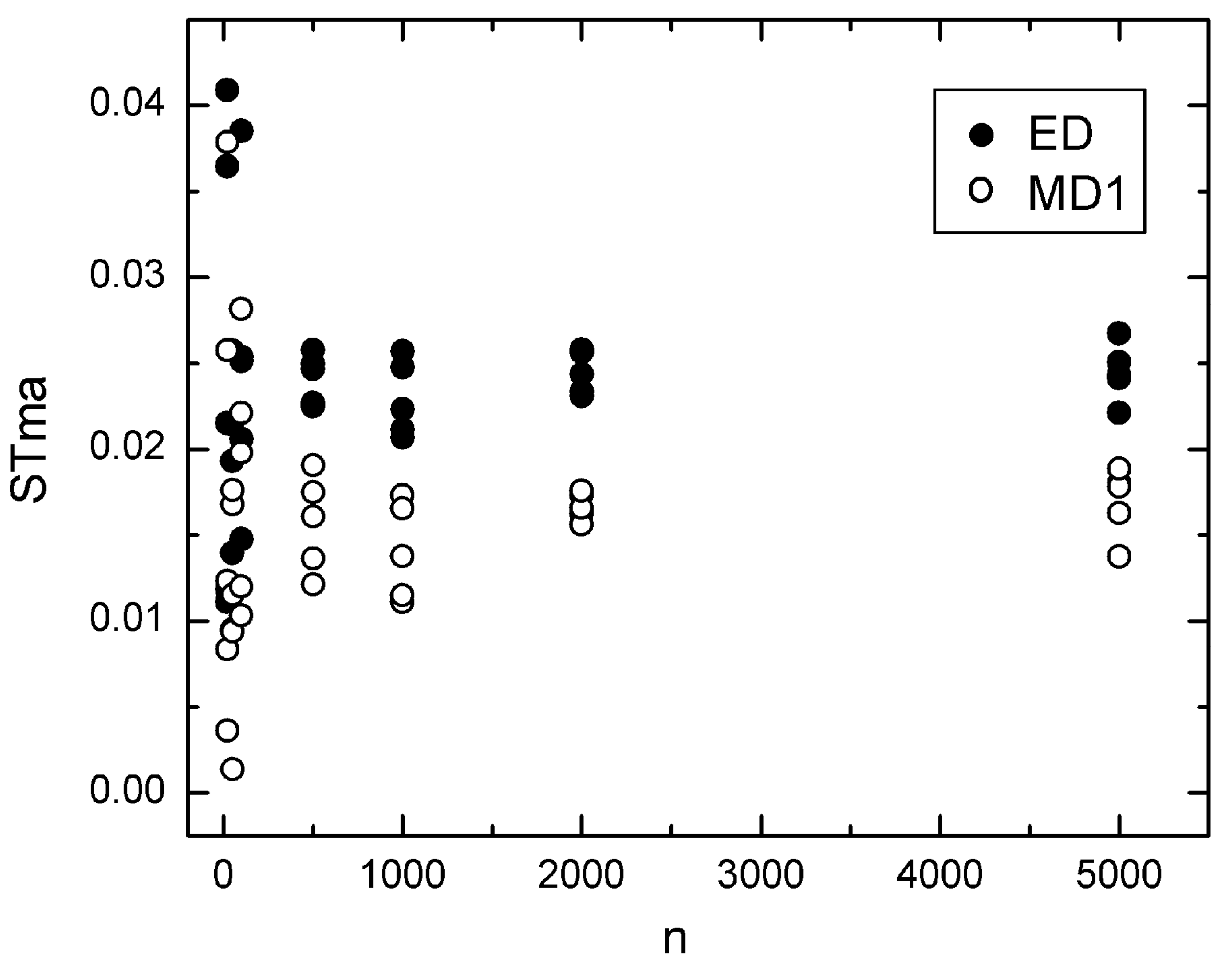
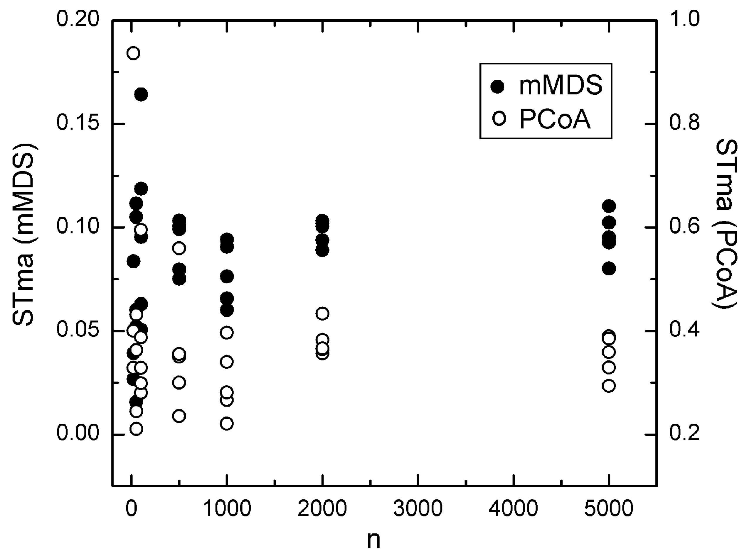
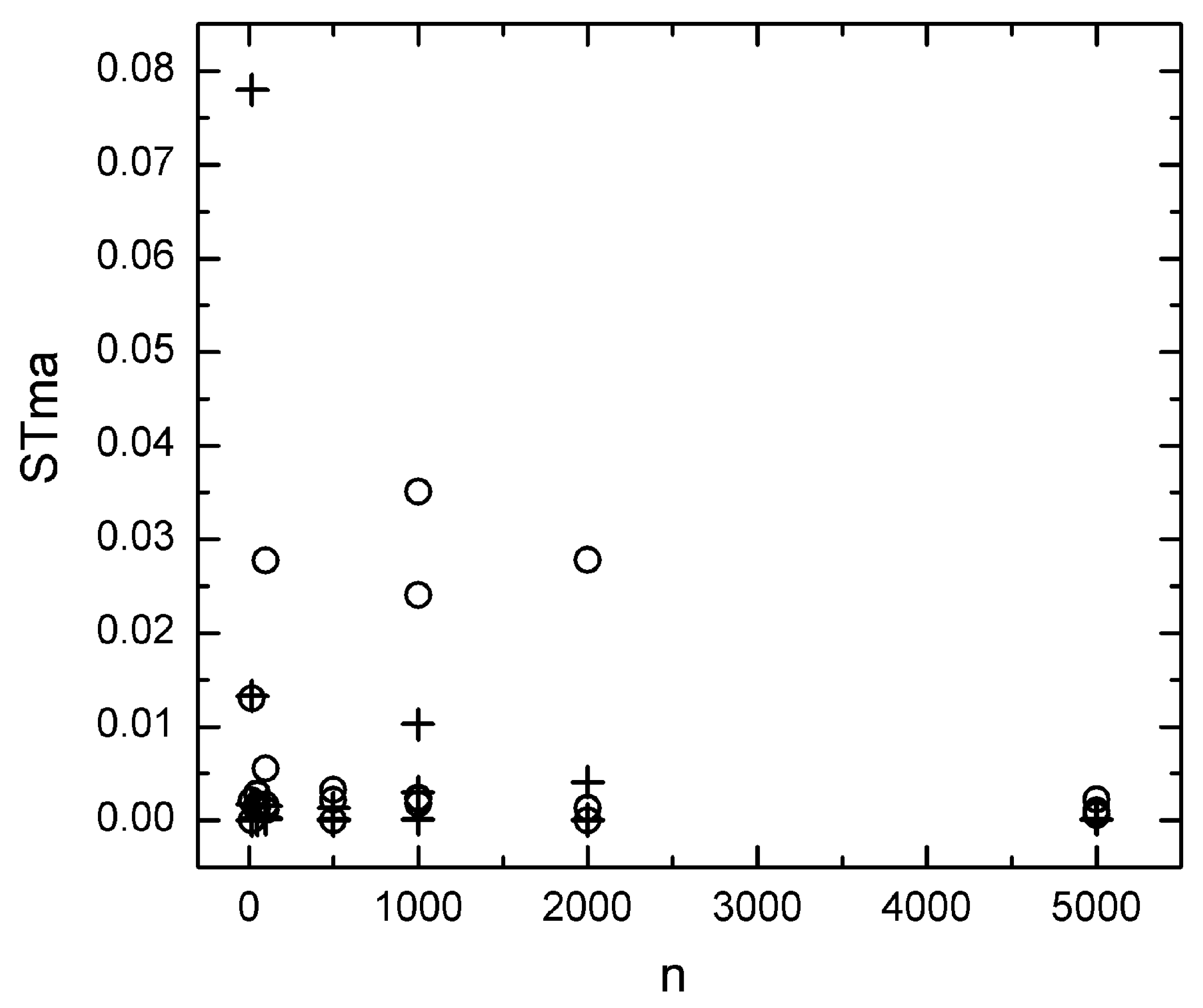
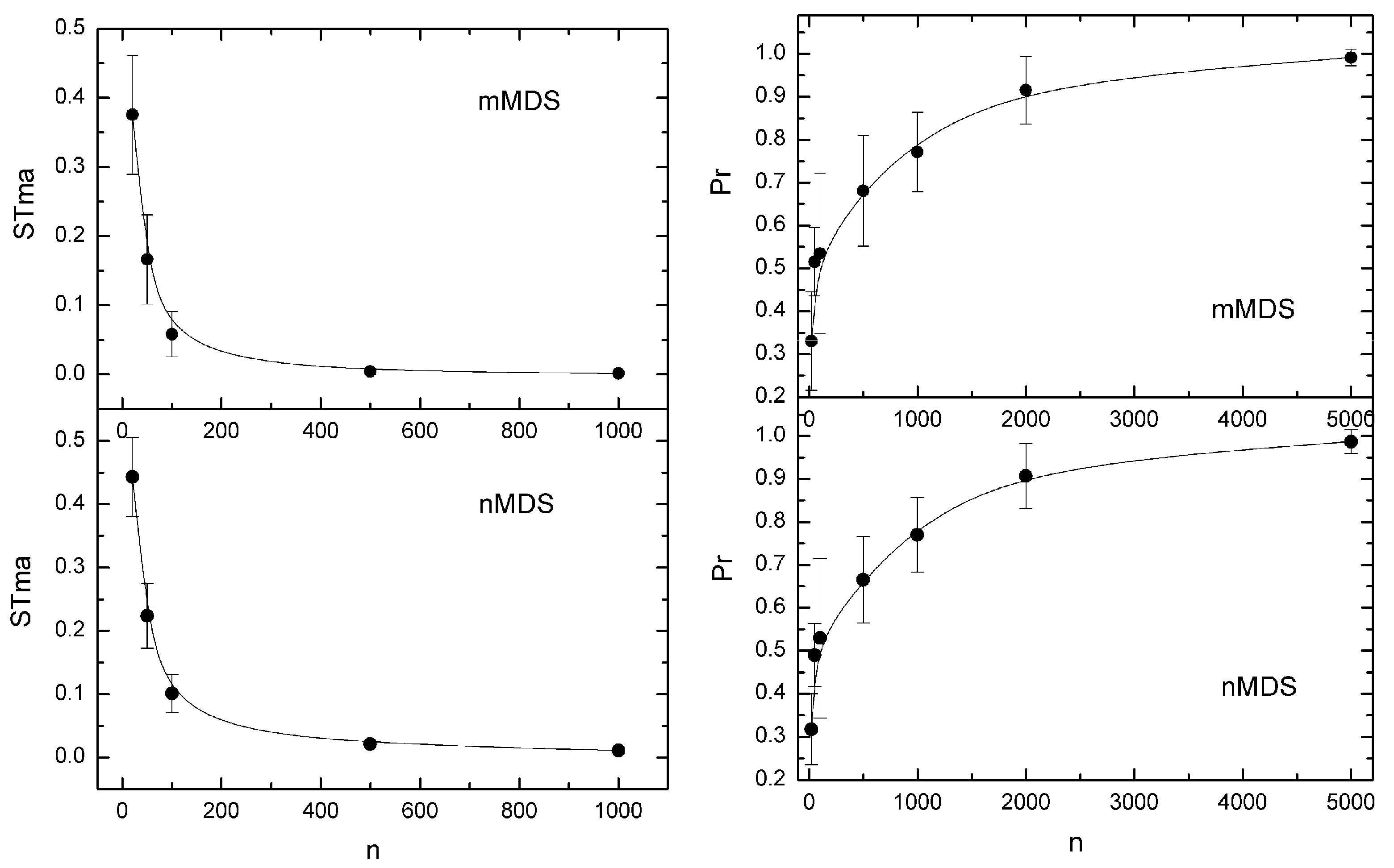
5.1. Effect of Sample Size

From the theory of the distances under study, we understand that their standard deviation decreases with increasing sample size, tending to zero as the sample size tends to infinity (see Supplement-S1-Moments in [15]). Therefore, when the sample size increases, the variability of the generated simulation distances decreases, resulting in smaller confidence intervals. That is, with great sample sizes, the confidence ellipses of the superimposed MDS solutions tend to become points that show the location of the populations in the MDS plot. Under these conditions, the probability of the most likely dendrogram obtained from the confidence ellipses tends to 1, and the same holds for its cluster probabilities. Thus, the uncertainty in a MDS plot, irrespective of whether it is assessed through the area of the ellipses or the corresponding dendrogram and its cluster probabilities, depends upon the size of the samples and tends to zero as that size tends to infinity.

Based on these observations, we examined the dependence of STma and the probability Pr of the most likely dendrograms upon the sample size in the simulated datasets. The most representative results are shown in Figure 1, Figure 2, Figure 3 and Figure 4. We observe that the stability measure STma calculated using the PCE method does not converge to zero when the sample size increases. Moreover, the value of STma obtained from PCE depends on the argument eps = ε. However, if we change eps, the plot in Figure 1 remains intact, and only the scale of the y-axis changes, but without a change in the position of the zero value. Similarly, the STma obtained from the BOOTres technique does not converge to zero when the sample size increases. Note that this property is also observed when using the conventional (not-squared) Euclidean distance. In addition, the ellipses generated from BOOTres using the corMDS technique largely overlap, yielding low STvr values. For example, the STvr is close to 1 when using the Euclidean distance and drops to around 0.3 and 0.45 when using the squared and not-squared Euclidean distances, respectively. This indicates that, in addition to nMDS, corMDS is also possibly incompatible with the BOOTres method. In any case, BOOTres and PCA do not calculate confidence ellipses.

Figure 3 shows the dependence of the stability measure STma upon sample size calculated from the JACKmds method using ordinal and ratio MDS of the ED distance. A decrease in STma is generally observed when the sample size tends to zero. However, extreme Stma values appear many times, almost in all sample sizes studied. Thus, zero STma values can appear even in small sample sizes, equal to 20 or 50, while particularly large values can also be observed. For example, in Figure 3, we can observe such large values when the sample size is equal to 1000 and 2000. Such extreme values have not been observed in any of the other methods examined and lead to a large amount of uncertainty regarding the accuracy of the method. Due to this uncertainty, its results should be treated with caution, and for this reason, it was not examined further.

Finally, in what concerns the MAPSov method, in all datasets examined, STma tends rapidly to 0 with the increase in the sample size (Figure 4—left). It was found that the dependence of STma on n follows the power model:

$$STma=A n^{-B}$$

(8)

with B > 0 and high R² fitting values, most of them around 0.99. As expected, this decrease in STma with the increase in n is associated with an increase in the probability of the most likely dendrogram, which tends to 1 (Figure 4—right). In most cases, the model that describes this increase is the logarithmic one $Pr=A ln\left(n\right)+B$. However, this tendency may be very slow, especially when the ED distance measure is used.

To sum up, of the four methods examined, BOOTres, PCE, JACKmds, and MAPSov, the first two do not calculate confidence ellipses, the JACKmds gives low precision confidence regions, and only the MAPSov method produces reliable MDS confidence ellipses, that is, confidence ellipses that tend to zero when the sample size increases; they do not exhibit extreme values, whereas their variability at a fixed n value is rather small (Figure 4—left). For these reasons, only the MAPSov method was selected for constructing confidence ellipses in MDS plots. At this point, we should also stress that, depending on the dataset, the performance of the MAPSov method may be affected by the MDS technique used. In fact, a satisfactory MDS technique should generate points within a confidence ellipse that are not spread away or form two or more accumulation regions but gather in a compact fashion within the elliptic region. Examining the various confidence ellipses involving MDS map points and constructed using the four MDS techniques adopted in the present study, we found that the most satisfactory of these techniques are the nMDS and PCoA.

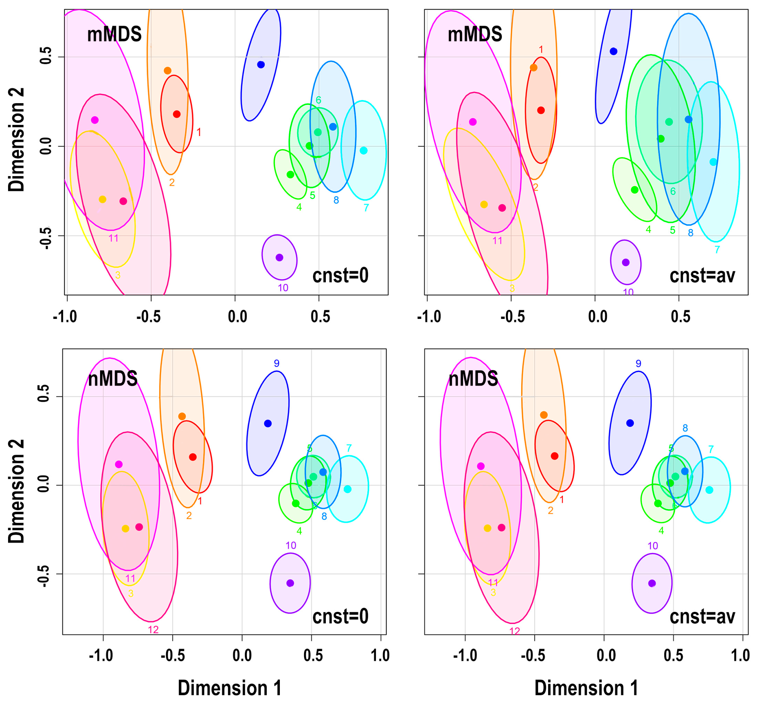
5.2. Effect of Adding a Constant

To examine the effect of adding a fixed value to the input distances, we have proceeded to the following qualitative and quantitative tests: The qualitative tests involved the visual inspection of plots of 95% confidence ellipses created with and without a fixed value added to the initial distances, like the plots in Figure 5. In the quantitative tests, we examined (a) the percent difference between the stability measures estimated with and without adding a constant and (b) the effect of the added constant on the cluster probabilities obtained from 95% confidence ellipses. Indicative quantitative tests are shown in

Table 1. Percent difference between the stability measures estimated with and without an added constant in the distance measures of the datasets EG1, EG2, and WH1.

		EG1	EG1	EG1	EG2	EG2	EG2	WH1	WH1	WH1
MDS	Stability	MD1-m	MD1-av	cMD1	MD1-m	MD1-av	cMD1	MD1-m	MD1-av	cMD1
mMDS	STvr	0.65	7.41	0.05	0.2	5.85	0.46	2.07	5.82	1.12
mMDS	STov	2.17	6.42	1.34	5.25	9.25	5.31	0.28	1.06	0.08
mMDS	STma	28.6	61.5	21.3	0.67	5.08	3.34	12.8	35.6	14.7
nMDS	STvr	0.52	4.67	0.14	0.02	1.04	0.09	0.01	0.05	0.01
nMDS	STov	1.02	3.80	0.88	2.46	6.96	2.03	0.02	0.01	0
nMDS	STma	8.53	23.9	4.84	0.18	8.02	0.07	0.34	1.00	0.28
PCoA	STvr	0.05	2.85	0.16	0.47	0.54	0.39	0.06	0.37	0.03
PCoA	STov	0.70	1.74	0.36	2.22	6.28	1.86	0.24	0.62	0.2
PCoA	STma	5.18	18.85	2.11	0.75	10.62	0.55	4.68	10.92	5.42
MDS	Stability	ED-m	ED-av	cED	ED-m	ED-av	cED	ED-m	ED-av	cED
mMDS	STvr	0.19	5.13	0.08	0.32	7.03	0.22	0.41	4.21	0.19
mMDS	STov	1.97	6.78	1.27	7.28	13.53	6.05	0.2	0.57	0.22
mMDS	STma	33.8	102.4	23.0	4.28	6.78	7.33	9.7	43.9	7.98
nMDS	STvr	0.22	3.3	0.02	0.61	0.31	0.11	0.02	0.05	0.04
nMDS	STov	1.3	4.11	0.99	4.38	13.5	2.61	0.04	0.16	0.03
nMDS	STma	10.14	39.5	5.32	0.45	6.21	1.89	0.94	3.74	2.08
PCoA	STvr	0.19	1.95	0.1	0.83	1.05	0.2	0.07	0.08	0.1
PCoA	STov	0.98	2.85	0.5	4.1	10.77	2.47	0.07	0.26	0.12
PCoA	STma	6.03	31.36	2.59	0.3	8.35	2.58	3.91	17.1	3.61

,

Table 2. As in Table 1 for the dataset NO1.

MDS	Stability	MMD	UMD	BMD1-m	BMD1-av	cBMD1
mMDS	STvr	3.04	2.64	5.87	11.6	4.89
mMDS	STov	0.97	1.12	2.98	6.70	0.60
mMDS	STma	0.41	1.0	6.03	8.48	2.65
nMDS	STvr	0.01	0.01	0.65	1.25	0.46
nMDS	STov	0.11	0.08	0.61	0.94	0.42
nMDS	STma	0.27	0.18	1.31	2.27	0.62
PCoA	STvr	0.23	0.21	1.41	3.07	0.28
PCoA	STov	0.55	0.65	0.06	0.78	0.34
PCoA	STma	0.8	0.67	1.06	1.83	0.54

Key: BMD1-m and BMD1-av denote values calculated when the added constant is the minimum and the average distance, respectively.

and

Table 3. Pearson correlation coefficients between cluster probabilities obtained from 95% confidence ellipses with and without an added constant in the distance measures of the datasets WH1 and NO1.

	WH1	WH1	WH1	NO1	NO1	NO1
MDS	MD1-m	MD1-av	cMD1	MMD	UMD	cBMD1
mMDS	0.9811	0.9037	0.9826	0.9966	0.9965	0.9951
nMDS	0.9989	0.9989	0.9992	0.9985	0.9970	0.9964
PCoA	0.9971	0.9847	0.9964	0.9975	0.9972	0.9968
MDS	ED-m	ED-av	cED	BMD1-m	BMD1-av
mMDS	0.9968	0.9266	0.9984	0.9868	0.9648
nMDS	0.9998	0.9995	0.9998	0.9972	0.9970
PCoA	0.9992	0.9715	0.9997	0.9952	0.9892

Key: MD1-m, ED-m, and BMD1-m denote values calculated when the added constant is the minimum distance, and MD1-av, ED-av, and BMD1-av denote values when the added constant is the average distance.

and Figure 6.

From all these tests, we obtained the following: In the datasets we studied, when the added constant is the minimum of the distances, the effect on the uncertainty in MDS is overall small irrespective of the MDS technique used. With the increase in the value of the added constant from the minimum value to the average value of the distances, alterations in the confidence ellipses may be detected. However, in this case, the effect of the added constant depends on the MDS technique used. In particular, this is almost insignificant for the nonmetric nMDS technique; it is rather small for the PCoA and becomes significant when using the metric mMDS. Note that the corMDS is not affected by adding a fixed value to the input distances. Noting that for the application of MDS with corrected Euclidean and Mahalanobis distances, as well as when using MMD and UMD, we add the absolute minimum value of the distance, we conclude that, in general, we can use any of the MDS techniques to construct confidence ellipses. However, since we cannot rule out the possibility of an extreme negative value, choosing nMDS, corMDS, or even PCoA, where the latter runs via the cmdscale() function of R, is safer.

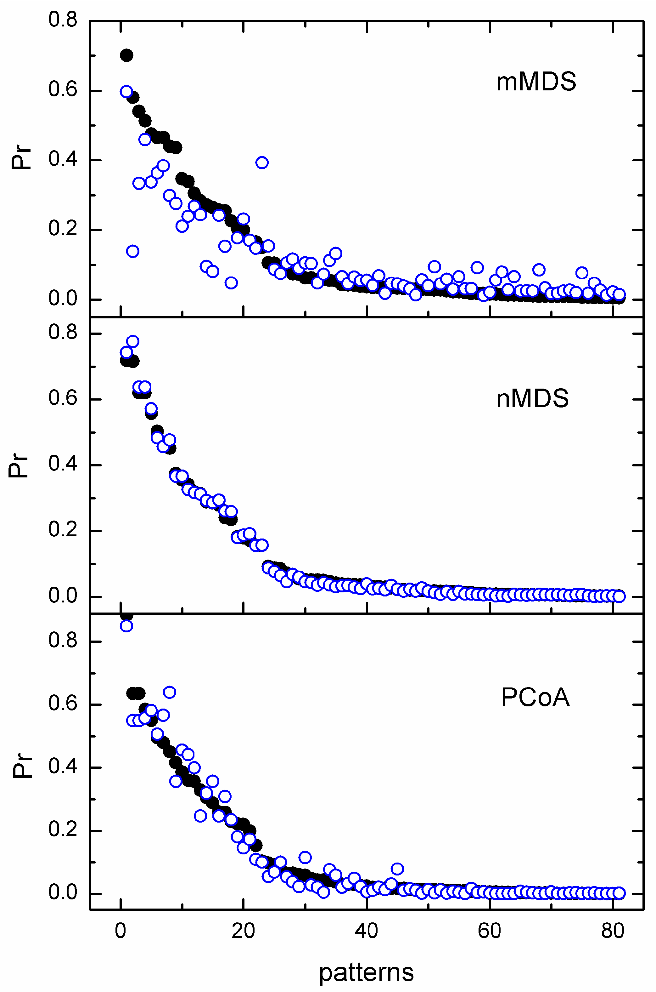
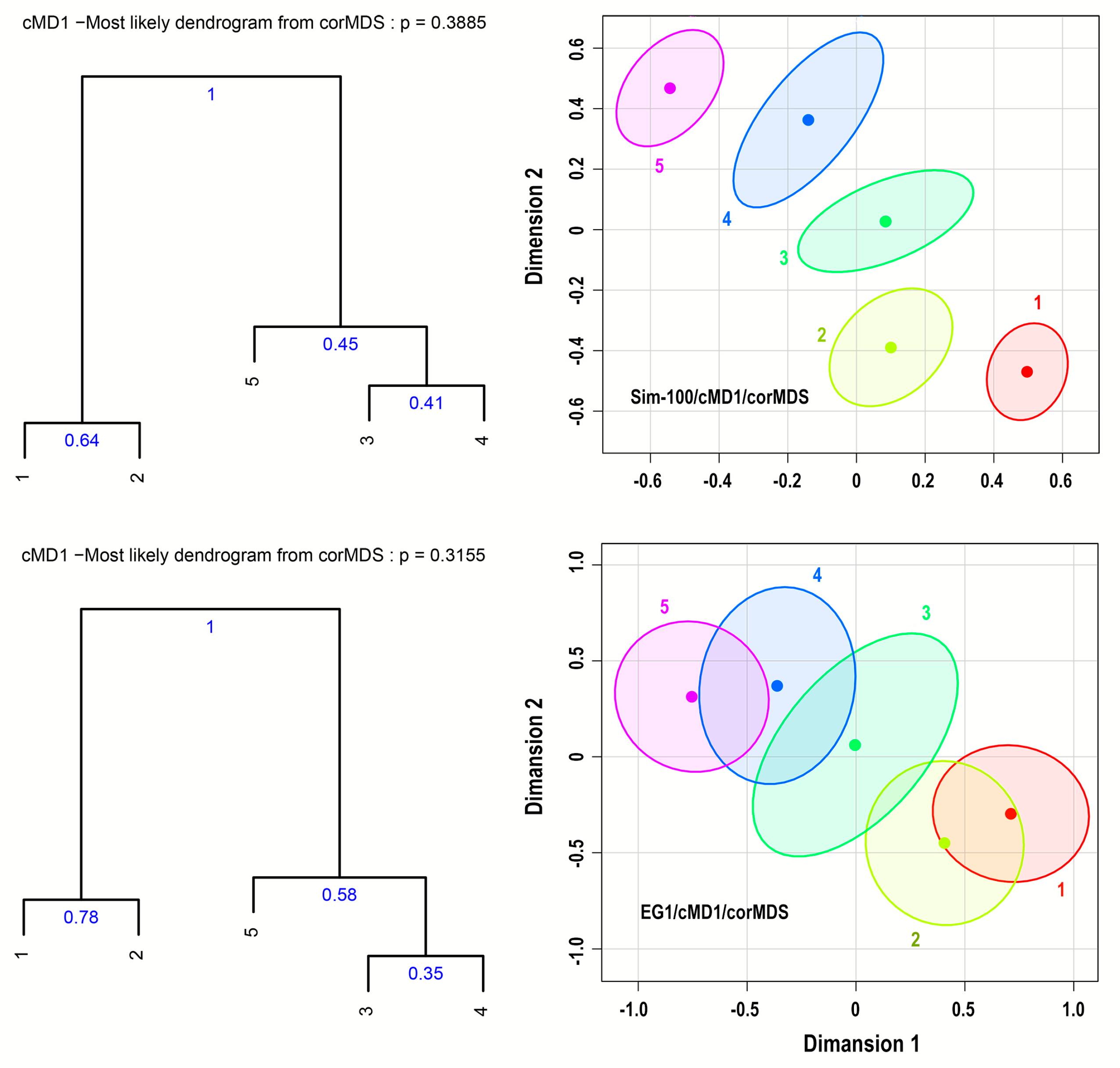
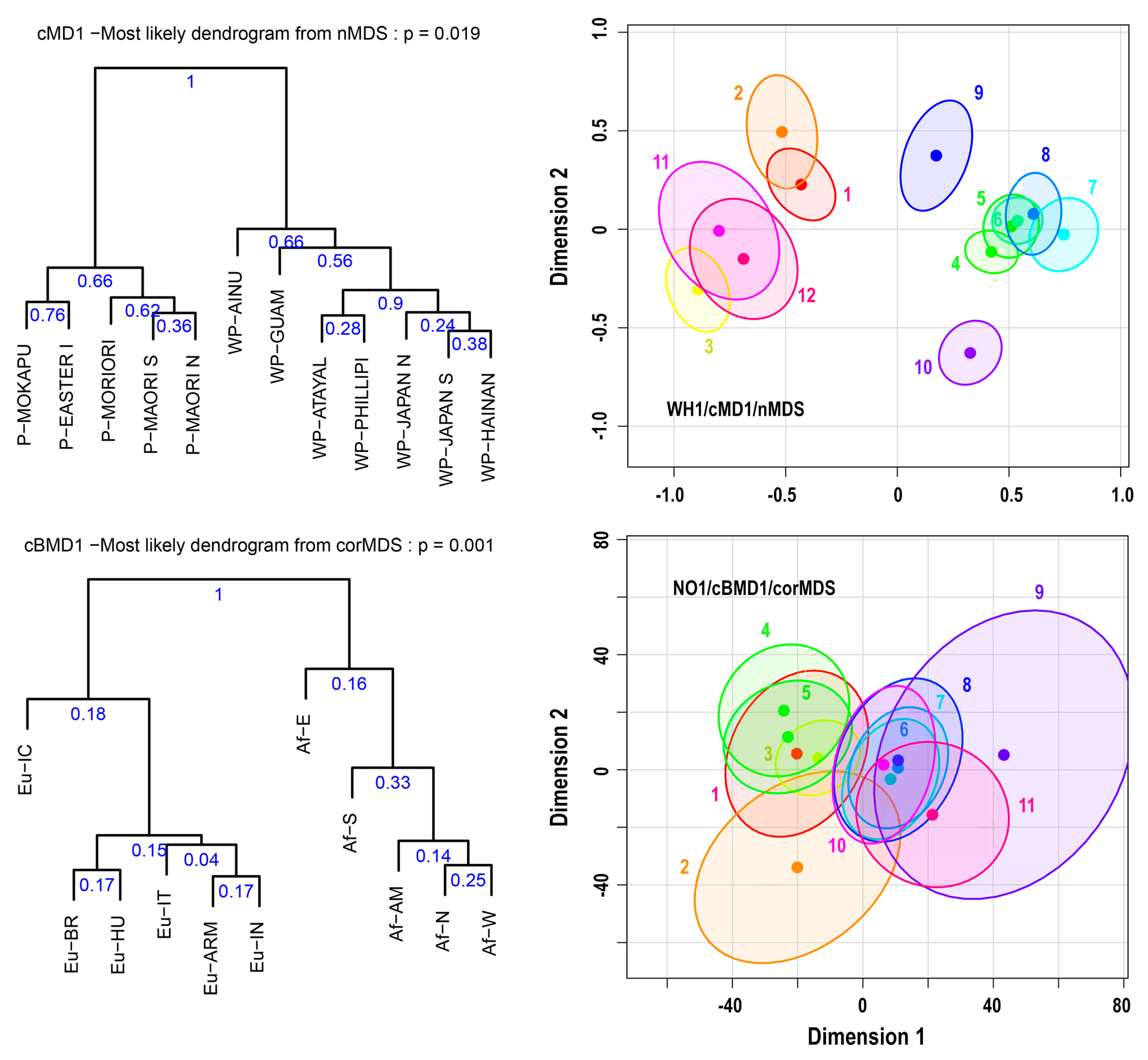
5.3. Confidence Regions and Cluster Probabilities

The MAPSov() function, using one or more pre-selected MDS methods and a certain distance measure, provides P% confidence ellipses along with the most likely dendrogram with its cluster probabilities obtained from these ellipses, the probability of its appearance, and the probabilities of the most frequent clusters. In addition, for comparison, the function provides similar information obtained from the direct application of HCA to the original dataset, that is, the basic dendrogram with its cluster probabilities, the probability of its detection, and various cluster probabilities, like the probabilities of the most frequent clusters. It can also provide the first m most likely dendrograms and their probabilities. Representative results are shown in Figure 7 and Figure 8 and in Supplement-S2-Tables and Dendrograms.

Figure 7 and Figure 8 show 95% confidence ellipses based on the corMDS or nMDS technique using the cMD1 or cBMD1 distance measures applied to the datasets EG1, Sim-100, WH1, and NO1. Note that the Sim-100 dataset is an artificial dataset that simulates the EG1 dataset using larger sample sizes, equal to 100. The figures also depict the corresponding most likely dendrograms with their probability, that is, the probability of their detection, and the Monte-Carlo cluster probabilities. More details related to Figure 7 and Figure 8 are provided in Supplement-S2-Tables and Dendrograms.

The general observation that comes from all MDS plots with 95% confidence ellipses is that the addition of these ellipses gives a much clearer picture of the biodistance map of the populations under study than the single points of the MDS plots. However, although they help to visualize the effect of uncertainty in the calculated distances on the distribution of populations on the MDS map, they do not eliminate subjective cluster selection based simply on the proximity of various MDS points. This step can be achieved only if we combine 95% confidence ellipses with HCA and, in particular, if we estimate cluster probabilities based on these ellipses.

Thus, if we consider Figure 7 and the corresponding results presented in the spreadsheets EG1 and Sim-100 in Supplement-S2-Tables and Dendrograms, we observe that for the dataset EG1, due to the rather small sample size, which is equal to 30, the 95% ellipses overlap, especially the ellipses of the sample pairs 1–2, 3–4, and 4–5, creating the impression that these pairs form pairwise clusters. This impression is enhanced by the high correlation between the percent of pairwise overlapping areas of 95% confidence ellipses and the corresponding cluster probabilities calculated from these ellipses. The Pearson and Spearman coefficients are 0.994 and 0.899, respectively, and, as expected, they are both statistically significant. Note that, similarly, the Pearson and Spearman coefficients between overlapping areas of 95% confidence ellipses and the corresponding cluster probabilities of the MDS plots of Figure 8 are high (>0.72) and statistically significant (spreadsheet Correlations in Supplement-S2-Tables and Dendrograms). However, this correlation is related to the uncertainty in the MDS plots and not to the presence of clusters. This can be seen if we look at low-uncertainty MDS plots, such as the plot in Figure 7 for the Sim-100 dataset. In such plots, the 95% confidence ellipses do not overlap, and, therefore, no correlation exists between overlapping areas and cluster probabilities. Moreover, at low-uncertainty MDS plots, the confidence ellipses may not help to determine clusters of samples. For example, we observe in Figure 7 that for the dataset Sim-100, the 95% confidence ellipses do not overlap and are approximately equidistant from each other. Therefore, we cannot confidently infer possible clusters among the samples. This can be done only via the estimation of Monte-Carlo pairwise cluster probabilities, especially the probabilities of the most frequent clusters/patterns.

The importance of the estimation of Monte-Carlo cluster probabilities is shown in both Figure 7 and Figure 8 as well as in the relevant spreadsheets in Supplement-S2-Tables and Dendrograms. In Figure 7, we observe that the most likely dendrogram of the dataset EG1 consists of the clusters (00110, 11000, and 00111), that is, the pairwise clusters 3–4 and 1–2 and the cluster 3–4–5 with probabilities of 0.35, 0.78, and 0.575, respectively, whereas similar is the case for the most likely dendrogram of the Sim-100 dataset. However, if we look at the probabilities of the most frequent clusters, we note that the 4–5 cluster (00011) has a significant probability equal to 0.6 for the dataset EG1 and 0.59 for Sim-100. Therefore, the MDS plots of EG1 and Sim-100 are very likely to be related to the clusters (11000, 00011, 00111), which are associated with the dendrogram obtained from the EG1 original dataset.

In Figure 8, at the MDS plot of WH1, we can easily distinguish at least three clusters: They are formed by the samples 1–2 (P-Mokapu, P-Easter I), 3–11–12 (P-Moriori, P-Maori S, P-Maori N), and 4–5–6–7–8 (WP-Japan N, WP-Japan S, WP-Hainan, WP-Atayal, WP-Phillipi) with probabilities of 0.76, 0.62, and 0.90, respectively. The samples WP-Guam and WP-Ainu seem to stand alone as outliers, but if we examine the cluster probabilities, these two samples can be clustered with the cluster (4–5–6–7–8). In this case, we have the formation of two clusters with probabilities of 0.66, corresponding to the classification of the samples as “Pacific” (P) and “West Pacific” (WP) [15]. Note that all the above clusters are depicted in the most likely dendrogram. In this dendrogram, as well as in the table of the most frequent cluster, we observe that there are many other clusters, but with probabilities less than 0.4. Therefore, it is not safe to draw conclusions about these clusters.

Figure 8 also shows the MDS plot of the dataset NO1. We observe that in this case, the uncertainty is so high that no safe conclusions can be drawn about clusters. Note that the high uncertainty is due to the nature of the dataset and not to the distance measure or the MDS technique used (see spreadsheet NO1 in Supplement-S2-Tables and Dendrograms). The best we can extract are two broad clusters, one with African and the other with Eurasian groups, with probabilities of only 0.16 and 0.18, respectively. Clusters with greater probability do exist, but they usually depend upon the distance measure used, except for the cluster between Af-S and Af-W, which has an average probability of about 0.31.

An interesting observation derived from Figure 8 and the relevant spreadsheets DetailsOnFigure 8 and NO1 in Supplement-S2-Tables and Dendrograms is the very low probability of the most likely dendrogram associated with a great number of dendrograms obtained from the MDS ellipses. This shows that the specific dendrograms, that is, dendrograms with a very low probability, have almost no value. Instead, the useful element of these dendrograms is the probabilities of the clusters that compose them. All these probabilities are presented by the MAPSov() function in the “Most frequent cluster probabilities from the ellipses of MDS” table.

Note that the MAPSov() function also presents (a) the probability of the basic dendrogram and the probabilities of the most likely dendrograms together with the probabilities of their clusters, and (b) the most frequent MC cluster probabilities estimated when HCA is applied to the original dataset (see spreadsheet NO1 in Supplement-S2-Tables and Dendrograms). Therefore, we can easily compare the information about the clusters obtained from the direct application of HCA to a dataset to that obtained from the application of the MDS technique.

Finally, we should point out that the reliability of the results regarding confidence ellipses and probabilities of clusters of samples depends upon the reliability of the simulated distances. For this reason, the MAPSov() function provides calculated sample distances (D), population distances (Dp), and simulated distances (Dsim) using Monte-Carlo or bootstrapping and averaged simulation distances (Dav). It was found that in all cases studied, the calculated sample distances (D) converged very satisfactorily with the simulated distances (Dsim) when using the Monte-Carlo method. Moreover, we found that in all corrected distances for small sample sizes (cED, cMD1, cMD2, MMD, UMD, and cBMD1), the population distances (Dp) converged satisfactorily with the averaged simulation distances (Dav). This property is not related to confidence ellipses and the estimation of reliable cluster probabilities but indicates that these distances are unbiased estimators of population divergence, which is a useful piece of information in biodistance studies.

6. Conclusions

The present paper first reviewed four stability methods for MDS plots, that is, methods proposed to evaluate the stability of MDS solutions, in order to choose the most appropriate one for producing reliable MDS confidence ellipses. It was found that the most effective of the methods studied is the MAPSov method, which involves the generation of simulated distances based on the original multivariate dataset and then the creation of MDS maps that are scaled, reflected, rotated, translated, and finally superimposed to construct confidence ellipses.

The MDS techniques used in the MAPSov method were the metric (mMDS) and nonmetric (nMDS) MDS based on the SMACOF algorithm, the metric MDS based on Principal Coordinates Analysis (PCoA), and an approach adopted in the present study based on the maximum correlation between initial and MDS distances (corMDS). The MAPSov method was used to assess the uncertainty in the MDS plots of squared Euclidean and Mahalanobis distances with and without correction for small sample sizes, as well as the corresponding distances for binary data. Since the correction for small sample sizes can lead to negative distance values, making it impossible to apply the MDS technique, the addition of a fixed value to the distances was thoroughly investigated. It was found that this addition is almost insignificant for the nonmetric nMDS technique, is rather small for the PCoA, and may become significant when using the metric mMDS. By construction, the corMDS is not affected by adding a fixed value to the input distances.

The application of the MAPSov method showed that the confidence ellipses in MDS plots of (bio)distances provide a good visualization of the (bio)distance map of the populations under study because they take into account the effect of the uncertainty in the computed distances on the distribution of the populations in the MDS map. This visualization is much better than that obtained from the single points of the MDS plots. However, to quantify the uncertainty and its effect on the determination of clusters of samples, we must apply the approach proposed in this paper. That is, we should apply hierarchical cluster analysis to the data of the 95% confidence ellipses and estimate all possible cluster probabilities related to these ellipses. This procedure can also be used to estimate the most probable dendrograms, their cluster probabilities, and the probability of their appearance.

References

1. Borg, I.; Groenen, P. Modern Multidimensional Scaling: Theory and Applications, 2nd ed.; Springer: New York, NY, USA, 2005. [Google Scholar]
2. Cox, T.F.; Cox, M.A.A. Multidimensional Scaling, 2nd ed.; Chapman and Hall: New York, NY, USA, 2001. [Google Scholar]
3. Johnson, R.A.; Wichern, D.W. Applied Multivariate Statistical Analysis, 4th ed.; Prentice-Hall: Upper Saddle River, NJ, USA, 1998. [Google Scholar]
4. Mair, P.; Groenen, P.J.F.; De Leeuw, J. More on Multidimensional Scaling and Unfolding in R: Smacof Version 2. J. Stat. Softw. 2022, 102, 1–47. [Google Scholar] [CrossRef]
5. De Leeuw, J. Pseudo Confidence Regions for MDS. 2019. Available online: https://rpubs.com/deleeuw/292595 (accessed on 15 October 2023).
6. De Leeuw, J.; Meulman, J. A special Jackknife for Multidimensional Scaling. J. Classif. 1986, 3, 97–112. [Google Scholar] [CrossRef]
7. Vicente-Villardon, J.L. Package ‘MultBiplotR’, Multivariate Analysis Using Biplots in R Version 1.3.30. 2021. Available online: https://cran.r-project.org/web/packages/MultBiplotR/MultBiplotR.pdf (accessed on 21 November 2023).
8. Ringrose, T.J. Bootstrapping and correspondence analysis in archaeology. J. Archaeol. Sci. 1992, 19, 615–629. [Google Scholar] [CrossRef]
9. Efron, B.; Tibshirani, R.J. An Introduction to the Bootstrap; Chapman and Hall: New York, NY, USA, 1993. [Google Scholar]
10. Milan, L.; Whittaker, J. Application of the parametric bootstrap to models that incorporate a singular value decomposition. Appl. Stat. 1995, 44, 31–49. [Google Scholar] [CrossRef]
11. Meulman, J.; Heiser, W.J. The Display of Bootstrap Solutions in MDS. Technical Report; Bell Laboratories: Murray Hill, NJ, USA, 1983. [Google Scholar]
12. Heiser, W.J.; Meulman, J. Constrained Multidimensional Scaling, including confirmation. Appl. Psych. Meas. 1983, 7, 381–404. [Google Scholar] [CrossRef]
13. Weinberg, S.L.; Carroll, J.D.; Cohen, H.S. Confidence regions for INDSCAL using the Jackknife and Bootstrap techniques. Psychometrika 1984, 49, 475–491. [Google Scholar] [CrossRef]
14. Jacoby, W.G.; Armstrong, D.A. Bootstrap confidence regions for Multidimensional Scaling solutions. Am. J. Polit. Sci. 2014, 58, 264–278. [Google Scholar] [CrossRef]
15. Nikita, E.; Nikitas, P. Simulation methods for squared Euclidean and Mahalanobis type distances for multivariate data and their application in assessing the uncertainty in hierarchical clustering. J. Stat. Comput. Sim. 2022, 92, 2403–2424. [Google Scholar] [CrossRef]
16. Suzuki, R.; Shimodora, H. Pvclust: An R package for assessing the uncertainty in hierarchical clustering. Bioinformatics 2006, 22, 1540–1542. [Google Scholar] [CrossRef] [PubMed]
17. Konigsberg, L.W. Analysis of prehistoric biological variation under a model of isolation by geographic and temporal distance. Hum. Biol. 1990, 62, 49–70. [Google Scholar] [PubMed]
18. Mahalanobis, P.C. On tests and measures of gronp divergence. J. Asiat. Soc. Bengal 1930, 26, 541–588. [Google Scholar]
19. Mardia, K.V.; Kent, J.T.; Bibby, J.M. Multivariate Analysis; Academic Press: San Diego, CA, USA, 1995. [Google Scholar]
20. McLachlan, G.J. Mahalanobis distance. Resonance 1999, 4, 20–26. [Google Scholar] [CrossRef]
21. Nikita, E. A critical review of the Mean Measure of Divergence and Mahalanobis Distances using artificial data and new approaches to estimate biodistances from non-metric traits. Am. J. Phys. Anthropol. 2015, 157, 284–294. [Google Scholar] [CrossRef] [PubMed]
22. Gower, J.C. Some distance properties of latent root and vector methods used in multivariate analysis. Biometrika 1966, 53, 325–338. [Google Scholar] [CrossRef]
23. Dryden, I.L.; Mardia, K.V. Statistical Shape Analysis; Wiley: Chichester, UK, 1998. [Google Scholar]
24. Gower, J.C. Generalized Procrustes analysis. Psychometrika 1975, 40, 33–50. [Google Scholar] [CrossRef]
25. Harris, E.F.; Sjøvold, T. Calculation of Smith’s mean measure of divergence for inter-group comparisons using nonmetric data. Dent. Anthropol. 2004, 17, 83–93. [Google Scholar] [CrossRef]
26. Ossenberg, N.S.; Dodo, Y.; Maeda, T.; Kawakubo, Y. Ethnogenesis and craniofacial change in Japan from the perspective of nonmetric traits. Anthropol. Sci. 2006, 114, 99–115. [Google Scholar] [CrossRef]
27. Thomson, A.; Randall-Maciver, R. Ancient Races of the Thebaid; Oxford University Press: Oxford, UK, 1905. [Google Scholar]
28. Egyptian Skulls. Available online: https://www3.nd.edu/~busiforc/handouts/Data%20and%20Stories/regression/egyptian%20skull%20development/EgyptianSkulls.html (accessed on 21 November 2023).
29. Howells, W.W. Cranial Variation in Man: A Study by Multivariate Analysis of Patterns of Difference among Recent Human Populations; Harvard University Press: Cambridge, MA, USA, 1973. [Google Scholar]
30. Howells, W.W. Skull Shapes and the Map: Craniometric Analyses in the Dispersion of Modern Homo; Harvard University Press: Cambridge, MA, USA, 1989. [Google Scholar]
31. Howells, W.W. Who’s Who in Skulls: Ethnic Identification of Crania from Measurements; Harvard University Press: Cambridge, MA, USA, 1995. [Google Scholar]
32. Howells, W.W. Howells’ craniometric data on the Internet. Am. J. Phys. Anthropol. 1996, 101, 441–442. [Google Scholar] [CrossRef] [PubMed]
33. The William W. Howells Craniometric Data Set. Available online: https://web.utk.edu/~auerbach/HOWL.htm (accessed on 21 November 2023).
34. Ossenberg, N.S. Cranial nonmetric trait database on the internet. Am. J. Phys. Anthropol. 2013, 152, 551–553. [Google Scholar] [CrossRef] [PubMed]
35. Cranial Nonmetric Trait Database, 2013. Available online: https://borealisdata.ca/dataset.xhtml?persistentId=hdl:10864/TTVHX (accessed on 21 November 2023).
Figure 1. Dependence of the stability measure STma upon n for the ED (●) and MD1 (o) distance measures when the PCE method for pseudo-confidence ellipses has been used with eps = 0.01.
Algorithms 16 00535 g001
Figure 2. Dependence of the stability measure STma upon n calculated using the BOOTres method for confidence ellipses along with the MD1 distance measure and the MDS techniques mMDS (●) and PCoA (o).
Algorithms 16 00535 g002
Figure 3. Dependence of the stability measure STma upon n calculated using the JACKmds method with an ordinal (o) and ratio (+) MDS of the ED distance.
Algorithms 16 00535 g003
Figure 4. (left). Dependence of the stability measure STma upon n calculated using the MAPSov method, the MD1 distance measure, and the mMDS and nMDS techniques. Points indicate values averaged over 5 datasets per n value. Bars show ± one standard deviation. Curves have been calculated from STma = 34.926 n−1.425 (mMDS) and STma = 8.7242 n−0.967 (nMDS) (right). Dependence of the probability of the most likely dendrograms upon n when they are created from data from confidence ellipses of the mMDS and nMDS techniques using MD1 simulated distances and the MAPSov method. Points indicate values averaged over 5 datasets per n value. Bars show ± one standard deviation. Curves have been calculated from Pr = 0.114 ln(n) + 0.0133 (mMDS) and Pr = 0.1154 ln(n) − 0.0124 (nMDS).
Algorithms 16 00535 g004
Figure 5. 95% confidence ellipses obtained from the WH1 dataset when using the distance measure MD1 and the mMDS and nMDS techniques. The added constant to the distance values is equal to 0 (left) and the average MD1 values (right). Populations: (1) P-Mokapu, (2) P-Easter I, (3) P-Moriori, (4) WP-Japan N, (5) WP-Japan S, (6) WP-Hainan, (7) WP-Atayal, (8) WP-Phillipi, (9) WP-Guam, (10) WP-Ainu, (11) P-Maori S, and (12) P-Maori N.
Algorithms 16 00535 g005
Figure 6. Cluster probabilities obtained from the confidence ellipses of mMDS, nMDS, and PCoA using the distance measure MD1 and the WH1 dataset. The added constant to the distance values is equal to 0 (●) and the average of the MD1 values (o).
Algorithms 16 00535 g006
Figure 7. 95% confidence ellipses based on the corMDS technique using the cMD1 distance measure on the EG1 and Sim-100 datasets and the corresponding most likely dendrograms with cluster probabilities.
Algorithms 16 00535 g007
Figure 8. 95% confidence ellipses based on the corMDS and nMDS techniques using the cMD1 and cBMD1 distance measures on the WH1 and NO1 datasets and the corresponding most likely dendrograms with cluster probabilities.
Algorithms 16 00535 g008