Article

White Blood Cell Classification: Convolutional Neural Network (CNN) and Vision Transformer (ViT) under Medical Microscope

by
Mohamad Abou Ali
1,
Fadi Dornaika
1,2,* and
Ignacio Arganda-Carreras
1,2,3,4
1
Department Computer Science and Artificial Intelligence, University of the Basque Country (UPV/EHU), Manuel Lardizabal, 1, 20018 San Sebastian, Spain
2
IKERBASQUE, Basque Foundation for Science, Plaza Euskadi, 5, 48009 Bilbao, Spain
3
Donostia International Physics Center (DIPC), Manuel Lardizabal, 4, 20018 San Sebastian, Spain
4
Biofisika Institute (CSIC, UPV/EHU), Barrio Sarriena s/n, 48940 Leioa, Spain
*
Author to whom correspondence should be addressed.
Algorithms 2023, 16(11), 525; https://doi.org/10.3390/a16110525
Submission received: 24 October 2023 / Revised: 9 November 2023 / Accepted: 13 November 2023 / Published: 15 November 2023
(This article belongs to the Special Issue AI Algorithms in Medical Imaging)

Abstract

:
Deep learning (DL) has made significant advances in computer vision with the advent of vision transformers (ViTs). Unlike convolutional neural networks (CNNs), ViTs use self-attention to extract both local and global features from image data, and then apply residual connections to feed these features directly into a fully networked multilayer perceptron head. In hospitals, hematologists prepare peripheral blood smears (PBSs) and read them under a medical microscope to detect abnormalities in blood counts such as leukemia. However, this task is time-consuming and prone to human error. This study investigated the transfer learning process of the Google ViT and ImageNet CNNs to automate the reading of PBSs. The study used two online PBS datasets, PBC and BCCD, and transferred them into balanced datasets to investigate the influence of data amount and noise immunity on both neural networks. The PBC results showed that the Google ViT is an excellent DL neural solution for data scarcity. The BCCD results showed that the Google ViT is superior to ImageNet CNNs in dealing with unclean, noisy image data because it is able to extract both global and local features and use residual connections, despite the additional time and computational overhead.

1. Introduction

Machine learning (ML) is a subfield of artificial intelligence (AI) that involves the development of algorithms capable of learning patterns and making predictions based on data. It is a broad field that encompasses different approaches and techniques, including deep learning (DL). Deep learning is a subset of ML that involves the use of artificial neural networks (ANNs) with multiple layers to learn patterns from data [1]. The neural networks in deep learning can have many layers, making it possible to extract complex features from data.
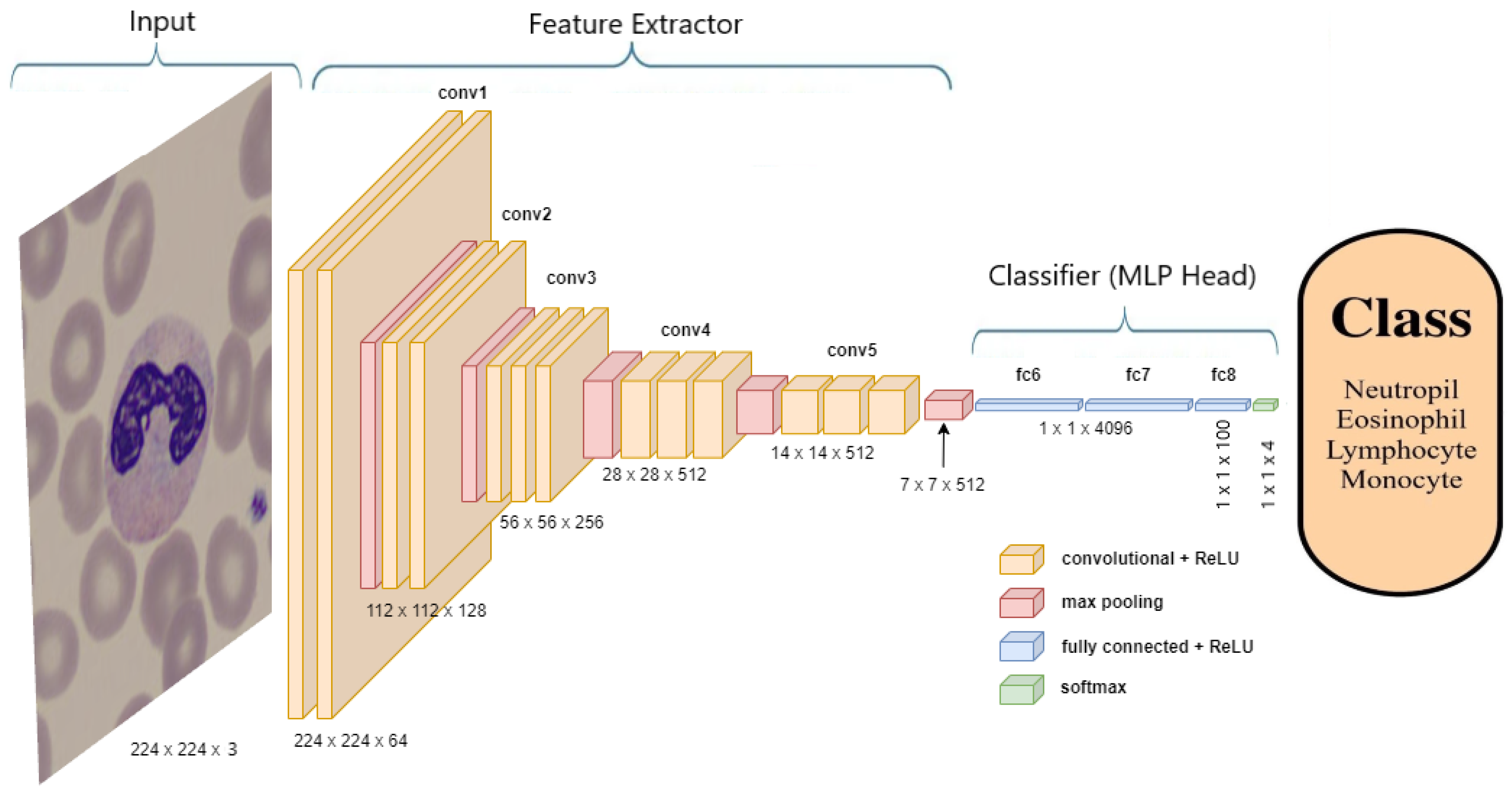
One popular application of DL is computer vision, where convolutional neural networks (CNNs) have proven to be very effective in image recognition tasks. CNNs use convolutional layers to extract features from images and pool those features to reduce the dimensionality of the data, allowing them to identify patterns and classify images into different categories [2].
Pre-trained CNN models are models that have already been trained on large datasets, such as the ImageNet dataset, making them useful for transfer learning on other datasets. Examples of such models are the winners of the ImageNet Large-Scale Visual Recognition Challenge (ILSVRC), including DenseNets, ResNets, and VGGs [3].
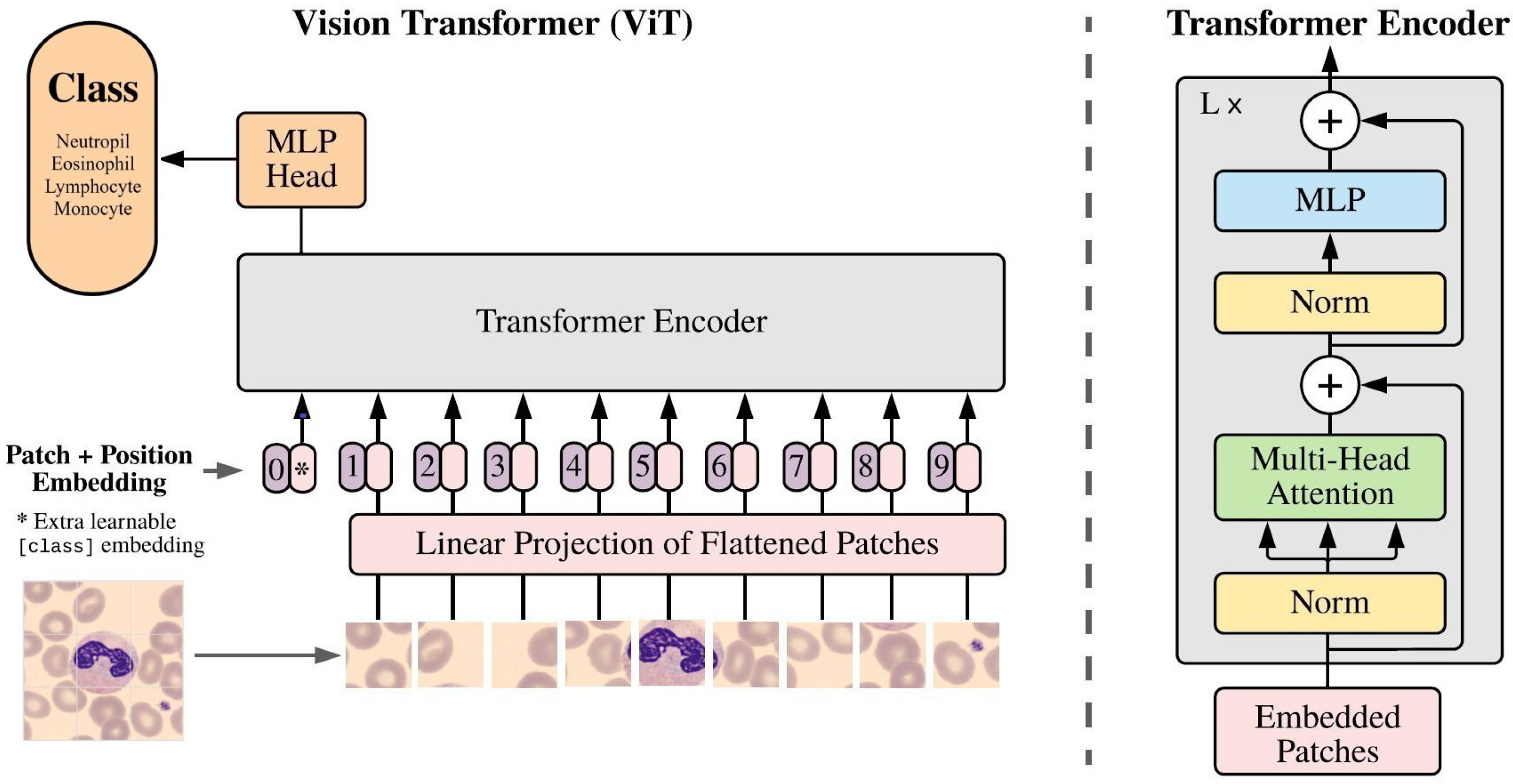
However, there has recently been growing interest in a new type of DL architecture called vision transformers (ViTs) [4], which are based on the transformer architecture commonly used in natural language processing (NLP) tasks. The ViT encoder uses a self-attention mechanism to extract features from the input image, allowing the model to consider the entire image at one time and identify important regions. This makes ViTs more efficient in identifying global features in images, such as overall shape and color, and permits them to learn more complex relationships between different parts of the image. Also, ViTs use residual links to forward extracted features to an MLP head unaffected by its depth.
This work aimed to investigate the performance and optimization learning of two deep neural networks, ImageNet CNNs and the Google ViT, in classifying four white blood cell (WBC) types (neutrophil, eosinophil, lymphocyte, and monocyte) by means of transfer learning. This study used the PBC [5] and BCCD [
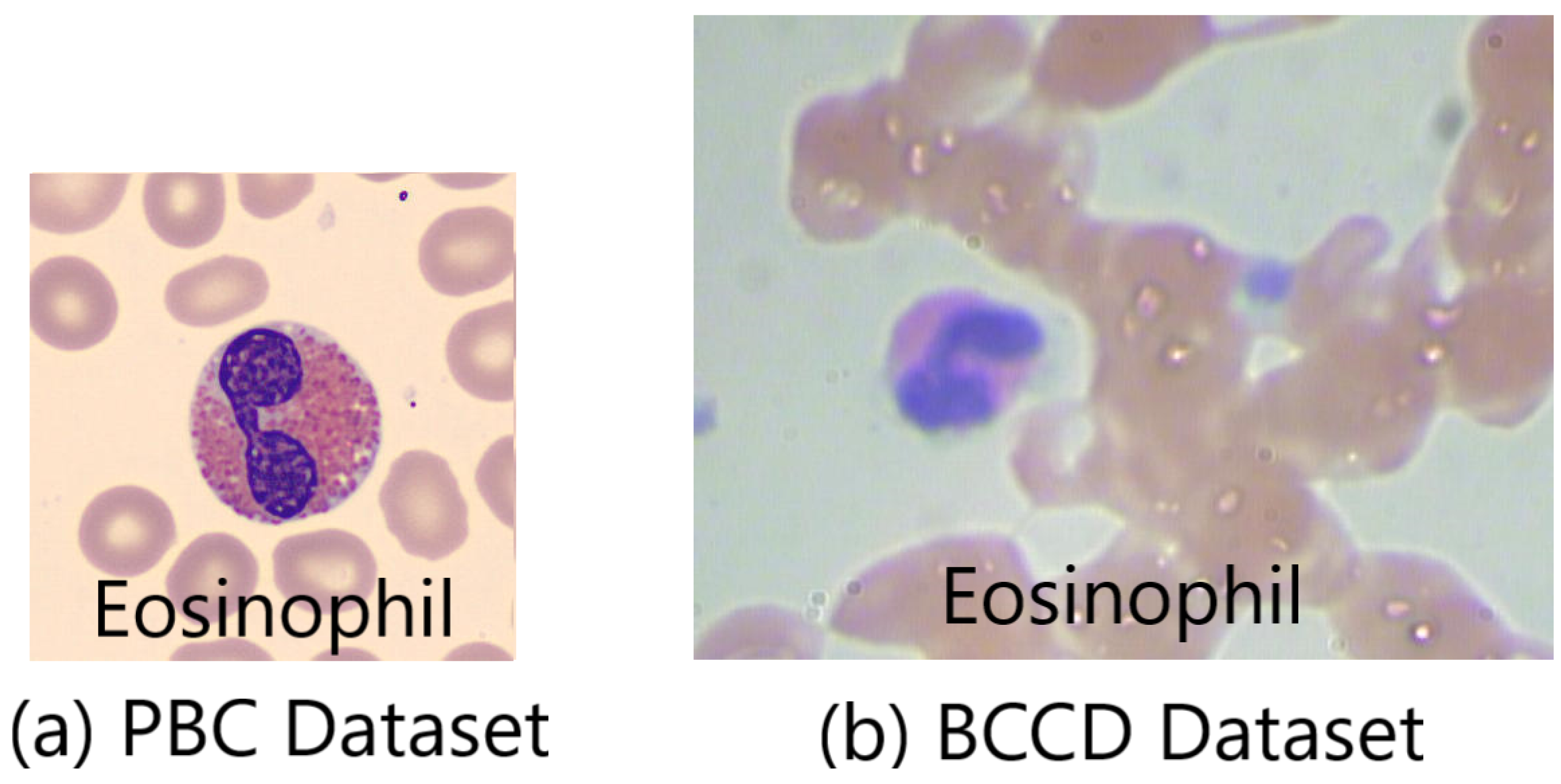
6] datasets. PBC is a large imbalanced dataset with high-quality images, while BCCD is a small imbalanced dataset with poor-quality images. Data augmentation techniques were employed to increase the size of the BCCD dataset.
The paper will proceed with a literature review of the relevant research related to the detection and classification of WBCs using pre-trained CNNs and ViTs in Section 2. Section 3 will describe the methodology used in this study, while Section 4 will present the experimental results obtained using pre-trained ILSVRC models and the Google ViT for blood cell classification. An in-depth analysis of the results will be provided in Section 5, and the paper will be concluded in Section 6.
Overall, the paper explores the effectiveness of pre-trained deep learning models in classifying WBC types from peripheral blood smear images. Transfer learning and data augmentation techniques were employed to address the imbalanced and poor-quality nature of the datasets. The results of the study can help improve the accuracy and efficiency of WBC classification, which could lead to the better diagnosis and treatment of blood disorders.

2. Related Works

Numerous research studies and publications have focused on the autonomous image analysis of white blood cells in microscopic peripheral blood smears. These studies leveraged transfer-based learning from pre-trained ImageNet models across various dataset sizes [7,8,9,10,11,12,13,14].
In their study [7], Sharma et al. employed convolutional neural networks, including a custom five-layer CNN (“LeNet-5”), and pre-trained models such as “VGGs”, “Inception V3”, and “Xception” for white blood cell classification. They tackled the challenging BCCD dataset, initially containing only 349 low-quality images distributed among four white blood cell categories: monocyte, lymphocyte, neutrophil, and eosinophil. Through extensive data augmentation techniques, they substantially expanded the dataset to over 3000 images per category. This augmented dataset was then divided into training and testing subsets, ultimately achieving an average classification accuracy of 87% for all four white blood cell types.
In a similar vein, Alam and Islam [8] also used the BCCD dataset for object identification considering red blood cells (RBCs), white blood cells (WBCs), and platelets. They divided the BCCD dataset into 300 images for training, reserving the remaining images for testing. The authors employed the Tiny YOLO model for object identification and incorporated pre-trained CNNs like VGG-16, ResNet-50, Inception V3, and MobileNet. Notably, all types of white blood cells were identified as WBC cells without further classification. However, no single model excelled in the identification of all RBCs, WBCs, and platelets simultaneously.
In another work [9], an automated system was introduced for classifying eight types of blood cells using convolutional neural networks (CNNs), specifically VGG-16 and Inceptionv3, with the PBC dataset. An impressive accuracy of 96.2% was achieved.
Jung et al. [10] introduced “W-Net”, a CNN-based architecture for classifying five different types of white blood cells. They utilized a dataset from the Catholic University of Korea (CUK), comprising 6562 images of these five WBC types. Additionally, the LISC dataset was used, and the pre-trained ResNet model was included for comparison. The results demonstrated that W-Net achieved an average accuracy of 97%.
In a different approach, a deep learning model using DenseNet121 was presented in [11] for classifying different white blood cell (WBC) types. The augmented BCCD dataset was employed, consisting of 12,444 images, including 3120 eosinophils, 3103 lymphocytes, 3098 monocytes, and 3123 neutrophils. Image pre-processing included the cropping of the WBC images. Then, augmentation techniques, such as flipping, rotation, brightness adjustment, and zooming, were applied to the isolated WBCs. The DenseNet121 model achieved an average accuracy of 98.84%.
Abou El-Seoud and colleagues [12] introduced a CNN-based architecture comprising five layers for classifying five types of white blood cells. They employed the BCCD dataset and applied augmentation techniques, including rotation, flipping, and shearing, to create a balanced training dataset with approximately 2500 images per class. The testing dataset contained fewer than 50 images, and the achieved average accuracy stood at an impressive 96.78%.
In their study [13], Sahlol and colleagues introduced a CNN-based architecture that utilized VGG-19 as a feature extractor and incorporated the Statistically Enhanced Salp Swarm Algorithm (SESSA) as an optimized classifier for categorizing five types of white blood cells (WBCs). Two datasets, the ALL-IDB and C-NMC datasets, were employed, resulting in an impressive average accuracy of 96.11%.
Almezhghwi and Serte [14] employed transfer learning with pre-trained CNNs like “ResNet”, “DenseNet”, and “VGG” to classify five types of white blood cells (WBCs) using a small dataset called LISC, which contained 242 images. They applied image segmentation to isolate WBCs and used data augmentation techniques, including data transformations and generative adversarial networks (GANs). The DenseNet-169 model achieved the highest average accuracy at 98.8%.
In this literature review, we examined a series of studies (Table 1) focusing on automating the classification of white blood cells in microscopic blood smears. These studies utilized diverse deep learning techniques, pre-trained models, and datasets, collectively showcasing the potential for precise white blood cell classification. The common thread across these works was the application of deep learning to enhance performance in this crucial medical domain.

3. Materials and Methods

This section describes the methodology adopted to classify the images of the four WBC types into different categories. Multi-class classification was performed using the pre-trained deep neural network models ImageNet ILSVRC and Google ViT [3,4]. Figure 1 shows a detailed methodology using the PBC dataset [5].
Figure 2 presents a detailed methodology using the BCCD dataset. An additional pre-processing step “data augmentation” was added to increase the size of the original BCCD dataset [6].

3.1. PBC and BCCD Datasets

3.1.1. PBC Dataset

The online “peripheral blood cells” dataset, known as the PBC dataset [5], includes 17,092 images of eight groups of blood cells: neutrophils, eosinophils, basophils, lymphocytes, monocytes, immature granulocytes, erythroblasts, and platelets (thrombocytes) (Table 2).
PBC images come with a standard size of 360 × 363 pixels, close to the input size of the ImageNet models and the Google ViT. This minimized the impact of downsizing the images.

3.1.2. BCCD Dataset

The BCCD dataset [6] originally contained 410 peripheral blood smear images including red blood cells (RBCs), WBCs, and platelets. The image format was JPEG with a size of 640 × 480. The Wright–Giemsa method was utilized to stain the blood smears, and the dataset was captured at a 100× magnification using a standard light microscope equipped with a CCD color camera.
Table 3 [6] presents a summary of the BCCD distribution of eosinophils, lymphocytes, monocytes, and neutrophils.

3.1.3. Dataset Quality and Size

Since the BCCD dataset had only four WBC classes (neutrophil, eosinophil, lymphocyte, and monocyte), this forced us to select only the same four WBC classes from the PBC dataset.
Figure 3 displays the huge difference in image quality between the PBC and BCCD datasets. It shows images of an eosinophil cell. The PBC eosinophil image [5] represents a well-prepared peripheral blood smear, which is free of noise, has a high resolution, and is full of details. This return back being automatically prepared and stained by the autostainer Sysmex SP1000i. On the other hand, the BCCD eosinophil image [6] shows a poorly manually prepared, stained, and captured peripheral blood smear, reflected by the noise, low resolution, and lack of detail.

3.2. Dataset Preprocessing

Dataset pre-processing usually consists of many steps, including image resizing, data augmentation, data balancing, and data splitting.

3.2.1. PBC Dataset Pre-Processing

The PBC dataset pre-processing included only three steps: image resizing, data balancing, and data splitting. First, images in the PBC dataset needed to be resized to fit the standard 224 × 224 image input of the pre-trained ImageNet ILSVRC and Google ViT models [3,4].
Secondly, the analysis of performance demanded that we kept the minimum number of evaluating metrics during the comparison. This target was achieved by employing balanced datasets with accuracy and loss as assessment tools. For this purpose, three balanced datasets (Table 4), DS-1, DS-2, and DS-3, were used to represent the PBC dataset.
The ultimate data pre-processing stage included partitioning the data into training and validation sets, with a distribution of 90% for training and 10% for validation for each new PBC dataset (Table 3).

3.2.2. BCCD Dataset Pre-Processing

The BCCD dataset pre-processing required the same steps as the PBC dataset with an additional data augmentation step to increase the amount of data. Table 2 shows that the number of WBC images in the BCCD dataset (four) was too small. Data augmentation techniques, such as image rotating and shearing, were randomly applied to produce enough data. Table 5 [6] represents a summary of the WBC distribution in the four newly created BCCD datasets, DS-4, DS-5, and DS-6.

3.3. Transfer Learning (TL)

Transfer learning (TL) is a common ML practice in computer vision whereby a model developed for one task serves as a starting point for a model aimed at a second task. Developers build on previous learning by leveraging already successful learning models, eliminating the need for a clean slate or starting from scratch. In addition, high performance is realized with small datasets and no expensive supercomputers [15].
First, in TL, a base network or a model is trained on a base dataset and task. Next, the learned features are transferred to a second target network or model for training on a target dataset and task. Accordingly, the TL process entails the existence of a pre-trained model, a model formed from an extensive set of reference data to solve a similar problem in another area [16,17].
Both pre-trained ImageNet ILSVRC and Google ViT models used an MLP head as a classifier. The output layer of the MLP head was removed, and a new output layer was added, representing the four WBC types of the PBC dataset.

3.3.1. ImageNet ILSVRC Models

The seven pre-trained ImageNet ILSVRC models considered in this research comprised two DenseNets (DenseNet-169 and DenseNet-201) [18]; InceptionResNet V2 [19]; three ResNets (ResNet-50, ResNet-101, and ResNet-152) V2 [20]; and VGG-16 [21]. Figure 4 represents a typical example of transfer learning for the seven pre-trained ImageNet ILSVRC models.
In Figure 4, the transfer learning process of the VGG-16 model is depicted. The weights of all layers, excluding the classifier (MLP Head), were held constant (“frozen”). The parameters of these layers in the feature extractor were designated as non-trainable. The only parameters subject to training during the fitting process were those associated with the classifier (MLP Head), revealing the new four-class WBC output layer.

3.3.2. Google Vision Transformer (ViT)

Figure 5a,b show the resizing of a 360 × 363 PBC neutrophil image into a 224 × 224 PBC neutrophil image. After that, Figure 5b,c demonstrate the splitting of the 224 × 224 neutrophil image into 196 patches using the standardized 16 × 16 patch size. However, Figure 3 shows the splitting of the neutrophil image into 9 patches instead of 196 patches, because the purpose in this figure was only graphical simplification.
In the Google ViT, similarly to the ILSVRC models, only the 1000-class output layer of the MLP head was replaced with the new four-class WBC output layer.
Figure 6 represents the transfer learning process of the Google ViT “ViTForImageClassification”.
However, all the parameters of the vision transformer entered into the training and validating process, and this justified the longer training time compared to the ILSVRC models.

3.3.3. Trial Setup

The AI tool used in this work was Google Colaboratory (“Google Colab” for short). Google Colab is a very useful product for ML and data analysis, allowing data scientists to write and execute Python code through an online-hosted Jupyter notebook [22].
The parameters kept constant during the trials were the Adam data optimizer, the categorical cross-entropy loss function, the accuracy metric, the epoch number of 10, and the 10-to-1 training-to-validating ratio.

3.3.4. Evaluation Metrics

The comparison of the ImageNet models and Google ViT was based on two types of learning curves: optimization and performance.
Optimization curves are a type of learning curve calculated based on the metric by which the model’s parameters are being optimized, such as loss or mean squared error (MSE).
In this work, categorical cross-entropy [23] was used as a loss function. Cross-entropy loss is used when adjusting model weights during training aiming to minimize the loss. This means that the smaller the loss, the better the model. A perfect model has a cross-entropy loss of zero. Cross-entropy [23] is defined in Equation (1) as follows:
L C E = i = 0 n t i log ( p i )
where t i is the truth label and p i is the Softmax probability for the ith class. Moreover, there are also two essential correlated terms associated with optimization curves: variance and overfitting.
Variance [24,25,26] is the difference in fit between the training and validating datasets. A high variance typically occurs when the model is too complex and does not reflect the simpler real patterns existing in the data. Variance is calculated using Equation (2):
σ 2 = 1 N i = 1 n ( x i x ¯ ) 2
where x i equals each value in the dataset, x ¯ is the mean of all values in the dataset, and N is the number of values in the dataset.
The training loss (TL) indicates how well the model fits the training data, while the validation loss (VL) indicates how well the model fits the new data. Variance is correlated with the loss difference (LD), which is the difference between VL and TL. The LD is calculated using the Equation (3):
LD = VL TL
Figure 7 [27] explains the underfitting and overfitting problems in relation training and validation losses. When the deep learning algorithm effectively captures the training data but performs poorly on the new data, it is unable to generalize, and this is known as overfitting. The greater the variance of a model, the more it overfits the training data.
As for performance learning, accuracy represents the ratio of true predicted classes to the total number of samples evaluated [28]. Equation (4) [28] demonstrates this computational process:
A c c u r a c y = T P + T N T P + T N + F P + F N
where TN and TP account for successfully classified negative and positive cases, respectively. Additionally, FN and FP report the number of misclassified positive and negative cases, respectively.
Another parameter used for performance assessment was the accuracy difference (AD) (5), i.e., the difference between the training accuracy (TA) and the validating accuracy (VA):
AD = VA TA
Apart from the previously mentioned metrics for model evaluation, another valuable tool employed for enhancing the interpretability of the models was Score-CAM [29]. Score-CAM is a visual explanation technique that utilizes class activation mapping (CAM) to assign scores to different regions in convolutional neural network (CNN) models, facilitating a deeper understanding of their internal workings.

4. Results

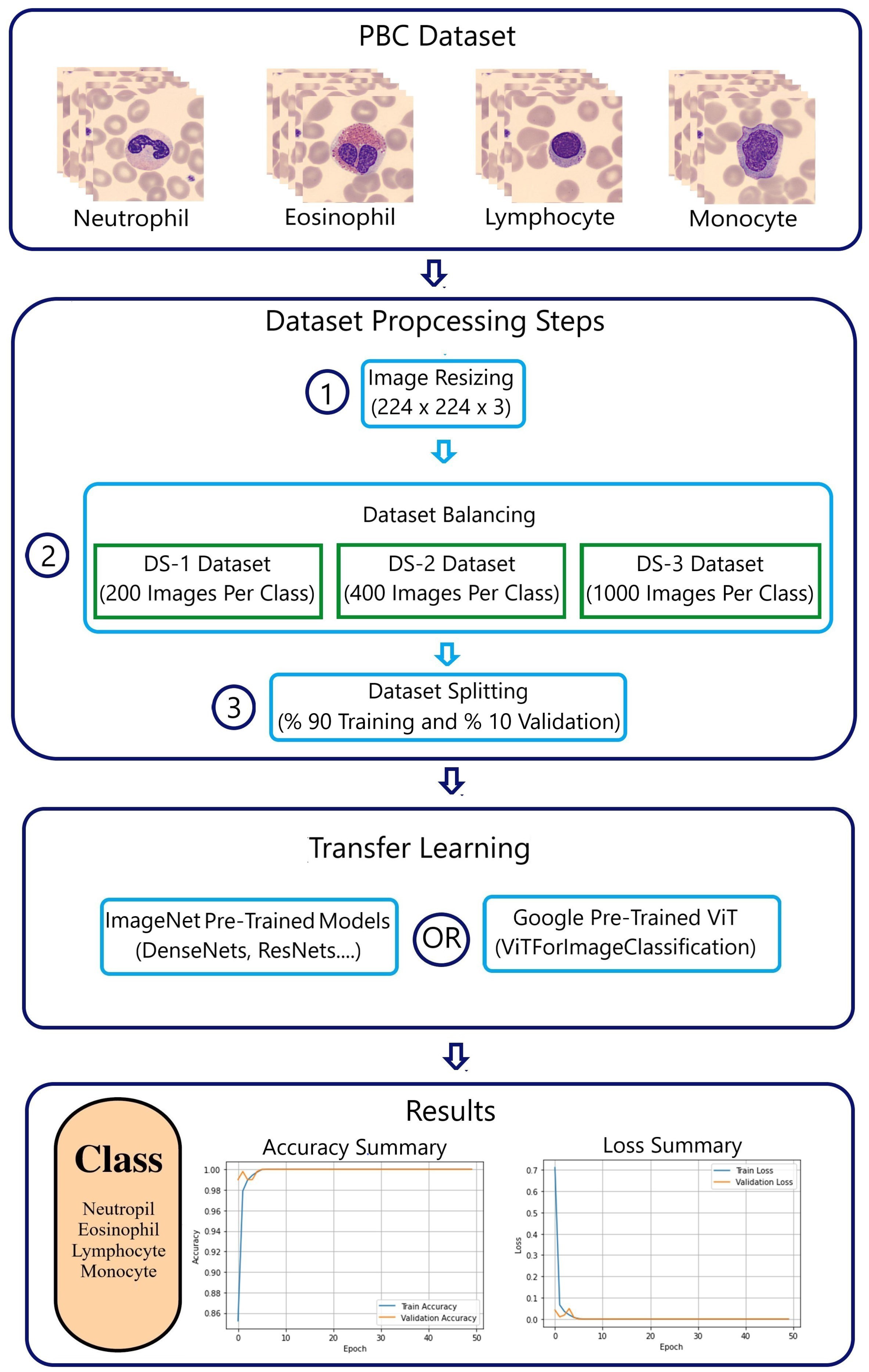
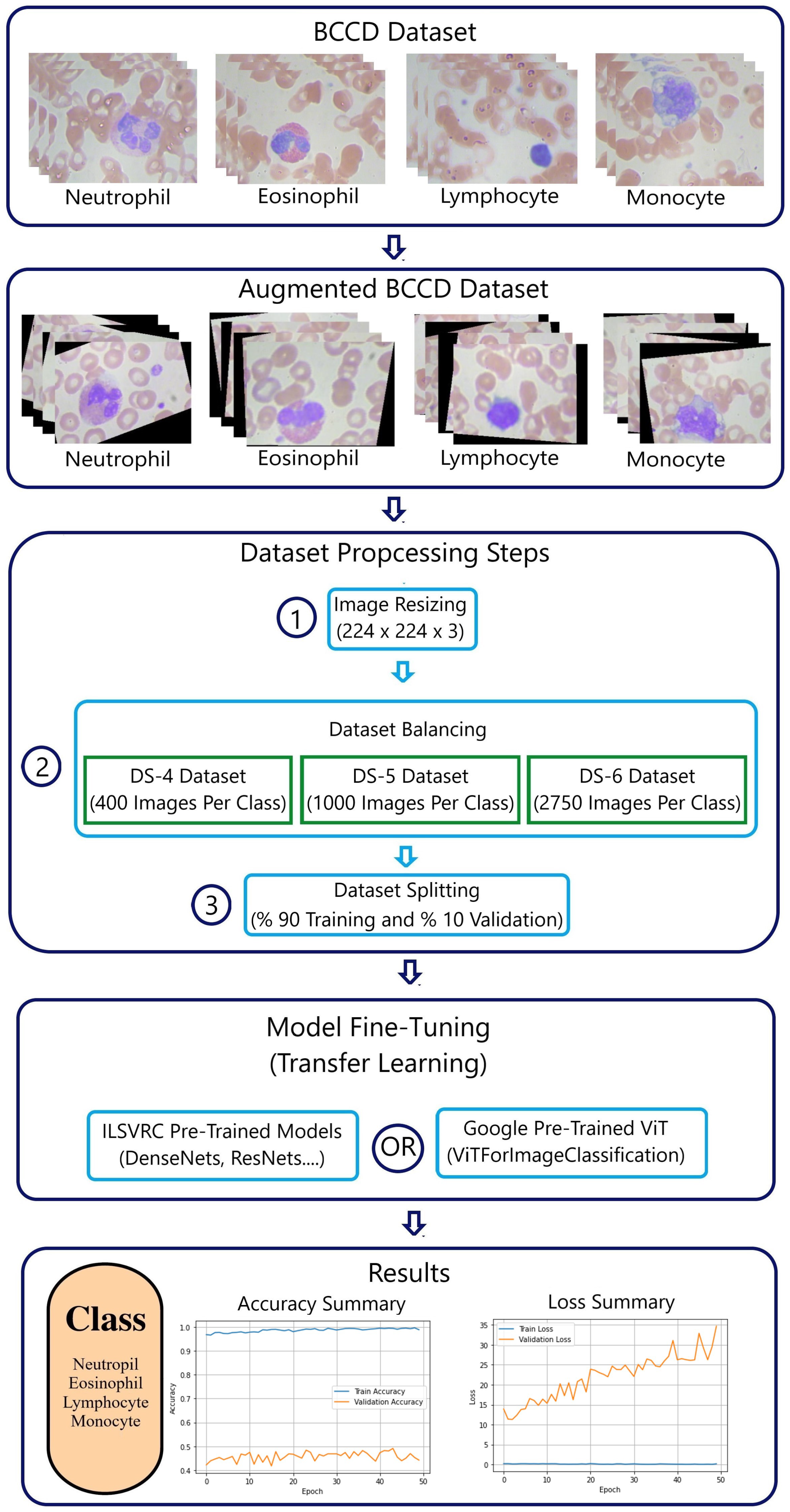
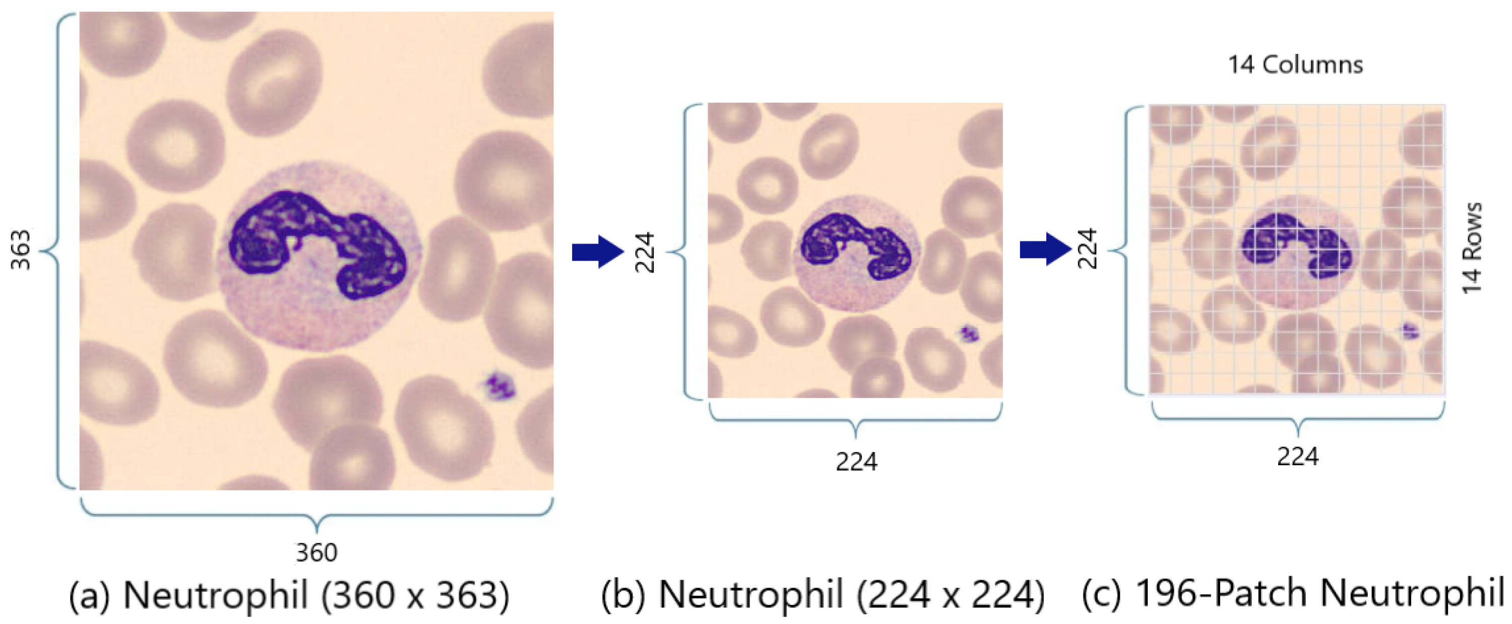
This section explains the experimental results for classifying WBC cells using the seven pre-trained ImageNet ILSVRC models and the Google ViTForImageClassification. The experiments were conducted on both the online peripheral blood smear PBC and BCCD datasets. The PBC dataset is characterized by being a large imbalanced dataset with standardized consistent high-quality images that are full of details, whereas the BCCD dataset is a small imbalanced dataset with blurred and noisy images due to the fact that the samples were manually prepared, stained, and captured.
In these experiments, the imbalanced PBC dataset was represented by three balanced datasets: DS-1 (200 images per class), DS-2 (400 images per class), and DS-3 (1000 images per class). Due to the small size of the BCCD dataset, data augmentation techniques were applied to increase the amount of data. Thus, the imbalanced BCCD dataset was embodied by three balanced datasets: DS-4 (400 images per class), DS-5 (1000 images per class), and DS-6 (2750 images per class). The dataset balancing was aimed at evaluating the ImageNet CNNs and Google ViT based on minimal metrics, namely accuracy and loss.

4.1. PBC Dataset Results

Table 6 shows the tenth-epoch validation accuracy and loss (VA and VL) values of the seven pre-trained ImageNet ILSVRC models versus the Google ViT. The Google ViT exhibited exceptionally stable performance compared to all ImageNet ILSVRC models. The Google ViT had a validation accuracy of 100 percent and a validation loss close to zero when fitted with the three PBC datasets (DS-1, DS-2, and DS-3).
As shown in Table 7, the Google ViT again outperformed all ILSVRC models, with an accuracy difference (AD) value of zero, representing the difference between the training and validating accuracies (TA and VA).
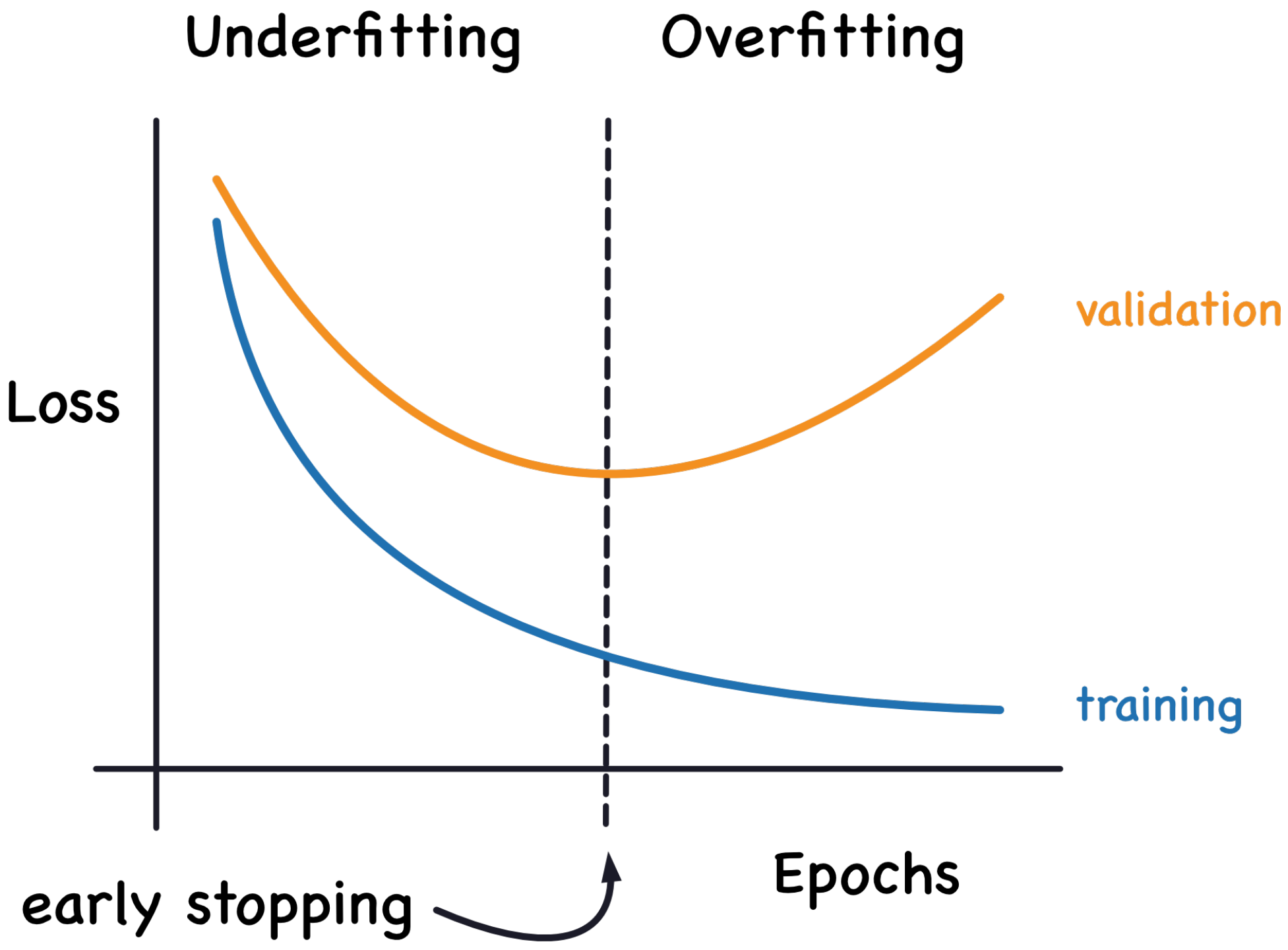
Table 8 clearly shows the development of an overfitting problem in all ILSVRC models due to the high variances caused by the high LD values when fitted using the DS-1 and DS-1 datasets. However, the size of the small and medium datasets DS-1 and DS-2 had no impact on the behavior of the Google ViT, which showed great results in such cases.
Finally, the larger number of trainable parameters for Google ViT compared to all ILSVRC models during the transfer learning process explained its need for additional computational resources and a longer training and validating time.

4.2. BCCD Dataset Results

Table 9 shows the tenth-epoch validation accuracy and loss (VA and VL) values of the seven pre-trained ImageNet ILSVRC models versus the Google ViT. The models were fitted with the three BCCD datasets (DS-4, DS-5, and DS-6). The Google ViT demonstrated better performance than all ImageNet ILSVRC models.
The Google ViT reached an 88.6% validation accuracy and a validation loss close to one when fitted with the BCCD DS-6 dataset. By comparison, when fitted with the DS-6 dataset, all ImageNet ILSVRC models displayed poor optimization learning and performance. This was due to the great amount of noise caused by the overuse of data augmentation and the poor quality of the original BCCD dataset images.
As shown in Table 10, the Google ViT fitted with the DS-6 dataset again outperformed the other models, reaching a +11.64% accuracy difference (AD) value, which was far better than any AD achieved by the ILSVRC models.
Table 11 clearly demonstrates that the Google ViT fitted with the DS-6 dataset again outperformed the other models, achieving a loss difference (LD) of around 1%, which was lower than any LD attained by the ILSVRC models.
Thus, Table 10 and Table 11 stress the same facts and conclusions supported by Table 9.

5. Discussion

The experimental results presented in this study provide valuable insights into the performance of the pre-trained ImageNet ILSVRC models and the Google ViT (vision transformer) when applied to the classification of white blood cells (WBCs). In this section, we discuss the key findings, implications, and limitations and provide a summary based on the results obtained from the PBC and BCCD datasets.

5.1. PBC Dataset Results

The results obtained from the PBC datasets demonstrated a stark contrast in the performance of the pre-trained ImageNet ILSVRC models and the Google ViT. The Google ViT consistently outperformed all ImageNet models across all three PBC datasets (DS-1, DS-2, and DS-3) in terms of both validation accuracy (VA) and validation loss (VL). It achieved a remarkable 100% validation accuracy and a validation loss close to zero. This exceptional performance suggests that the Google ViT is well-suited for handling imbalanced datasets with high-quality, detailed images.
Furthermore, when we analyzed the accuracy difference (AD) values, it was evident that the Google ViT maintained a constant 0% AD across all three PBC datasets. In contrast, the ImageNet models exhibited positive AD values, indicating overfitting issues, especially when working with the DS-1 dataset. This overfitting was likely due to the high variances caused by the presence of limited data in DS-1. The Google ViT’s consistent performance regardless of dataset size suggested its robustness in dealing with small and medium-sized datasets.
The LD (loss difference) values further emphasized the Google ViT’s superiority. While the ImageNet models displayed varying degrees of loss difference as the dataset size increased, the Google ViT consistently maintained minimal loss differences, once again highlighting its stability.
Overall, the performance of the Google ViT on the PBC datasets indicated its effectiveness in handling large, imbalanced, and high-quality image datasets while mitigating overfitting issues.

5.2. BCCD Dataset Results

In contrast to the PBC datasets, the BCCD datasets presented a more challenging scenario due to their small size, noise, and poor image quality. The Google ViT continued to demonstrate its superior performance, achieving an 88.36% validation accuracy and a validation loss close to one when fitted with the BCCD DS-6 dataset. This exceptional performance, especially when handling the most challenging dataset, DS-6, is a testament to the robustness of the Google ViT.
When compared to the ImageNet models, the Google ViT was consistently superior across all three BCCD datasets (DS-4, DS-5, and DS-6) in terms of the accuracy difference (AD) and loss difference (LD) values. The AD values for the Google ViT were consistently lower, indicating its ability to maintain a higher accuracy. In addition, the LD values for the Google ViT remained minimal, underscoring its stability even when dealing with small, noisy, and low-quality image datasets.
The superior performance of the Google ViT on the BCCD datasets, especially the DS-6 dataset, highlights its resilience in the face of challenging data conditions and noise. This makes it a promising choice for applications where image quality is a concern or where the dataset size is limited.

5.3. Score-CAM

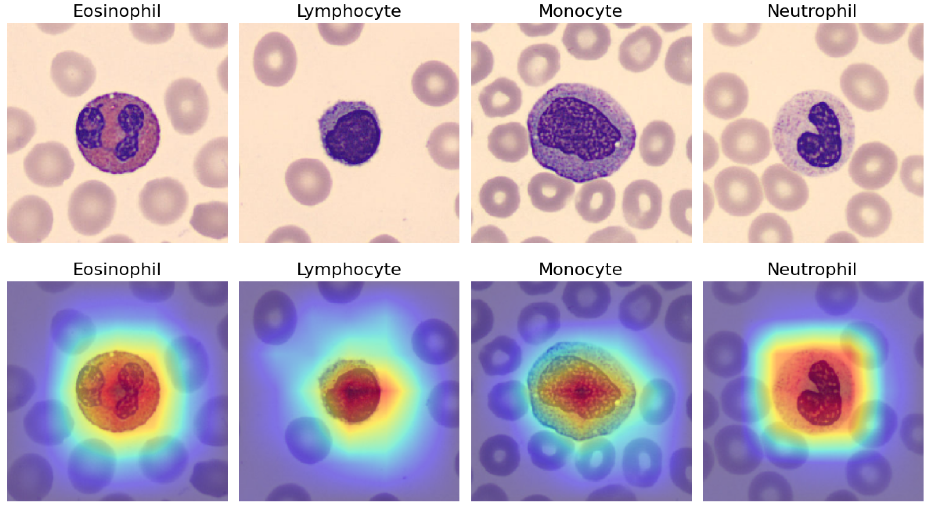
These findings received additional support from the utilization of Score-CAM, as depicted in Figure 8, which offers a visual representation of the fitted pre-trained DenseNet-169 model’s performance using the DS-3 PBC dataset. In Figure 8, four selected WBCs, namely an eosinophil, lymphocyte, monocyte, and neutrophil, randomly taken from the DS-3 PBC dataset, are presented in the upper section. Meanwhile, the lower section of Figure 8 displays their corresponding Score-CAM images, highlighting the specific areas of focus detected by the DenseNet-169 model.

5.4. Implications and Limitations

The findings in this study have significant implications for the field of deep learning and computer vision. The Google ViT’s consistent and exceptional performance, even on challenging datasets, suggests its potential for a wide range of medical image analysis and diagnostic applications. Its robustness to dataset size and quality could lead to more accurate and reliable results in various healthcare settings, providing valuable support for medical professionals.
One of the strengths of this study was its focus on key metrics such as accuracy, loss, accuracy difference (AD), and loss difference (LD), which provided a comprehensive evaluation of the models’ performance. The results were clear and consistent across all datasets, supporting the conclusion that the Google ViT is a powerful choice for medical image classification tasks.
This work featured many novel aspects and perspectives when compared to the previously cited works [7,8,9,10,11,12,13,14].
Firstly, it utilized the Google ViT for the first time and proved its superiority in performance and stability compared to the ImageNet CNNs under the same circumstances and conditions. The Google ViT achieved superior performance, with an average 100% accuracy. Secondly, this work shed light on and stressed the significance of data processing techniques, such as data balancing, in order to achieve better performance and a higher accuracy. Additionally, it demonstrated the negative impacts of poor data processing habits, such as the overuse of data augmentation methods without considering the preservation of an acceptable ratio between the original data and their augmented versions. Finally, it clearly showed how such a case could be exaggerated in the event of unclean noisy image data.
One limitation of our study lay in its exclusive focus on the classification of four mature WBC types. This raises the question of whether our findings would hold true if additional blood cell classes, such as basophils; segmented/banded neutrophils; immature granulocytes (pro-myelocytes, myelocytes, meta-myelocytes); and erythroblasts, were included. The inclusion of these additional cell classes could significantly increase the complexity of the classification task due to their numerous similarities, presenting a challenging avenue for future research.

5.5. Summary

In summary, the experimental results from this study demonstrated that the Google ViT consistently outperformed the pre-trained ImageNet ILSVRC models when classifying white blood cells (WBCs), even when dealing with challenging datasets. Its exceptional stability, regardless of dataset size or image quality, highlights its potential for various medical image analysis tasks. Researchers and practitioners in the field of medical imaging should consider the Google ViT as a reliable and robust tool for image classification tasks, particularly in healthcare applications. This study emphasizes the importance of selecting the right deep learning model to achieve high performance in medical image analysis and paves the way for further advancements in the field.

6. Conclusions

In conclusion, this study thoroughly assessed the performance of the Google ViT when classifying four types of WBCs using peripheral blood smear images from two online datasets, the PBC and BCCD datasets. To address data scarcity, the study employed three balanced datasets (DS-1, DS-2, and DS-3) from the PBC dataset, which contained high-quality images of various blood cell groups. The Google ViT exhibited superior performance compared to the ImageNet CNNs when dealing with data shortages. Furthermore, the study applied data augmentation techniques to create three balanced datasets (DS-4, DS-5, and DS-6) from the low-quality BCCD dataset, introducing noise to the data. In this scenario, the Google ViT demonstrated its robustness and resilience to noisy data, in contrast to the ImageNet CNNs. In summary, this work underscored the effectiveness of ViTs in scenarios of data insufficiency and the presence of unclean data.
In future research, we will expand the scope of this study to encompass additional blood cell classes, including basophils; segmented/banded neutrophils; immature granulocytes (pro-myelocytes, myelocytes, meta-myelocytes); erythroblasts; and other related cell types. These additional classes exhibit notable similarities among themselves. Additionally, our study will aim to augment the number of images within each class to provide a more challenging task for both ViTs and pre-trained CNNs.

Author Contributions

Conceptualization, M.A.A. and F.D.; methodology, M.A.A. and F.D.; software, M.A.A.; validation, M.A.A.; formal analysis, M.A.A., F.D. and I.A.-C.; investigation, M.A.A.; resources, M.A.A. and F.D.; data curation, M.A.A.; writing—original draft preparation, M.A.A. and F.D.; writing—review and editing, M.A.A., F.D. and I.A.-C.; supervision, F.D. and I.A.-C.; project administration, F.D. and I.A.-C.; funding acquisition, F.D. and I.A.-C. All authors have read and agreed to the published version of the manuscript.

Funding

This work is supported by grant PID2021-126701OB-I00 funded by MCIN/AEI/10.13039/501100011033 and by “ERDF A way of making Europe”, and by grant GIU19/027 funded by the University of the Basque Country UPV/EHU.

Data Availability Statement

The data used in this paper are publicly available.

Conflicts of Interest

The authors declare that the research was conducted in the absence of any commercial or financial relationships that could be construed as a potential conflict of interest.

References

  1. Mishra, C.; Gupta, D.L. Deep machine learning and neural networks: An overview. IAES Int. J. Artif. Intell. (IJ-AI) 2017, 6, 66. [Google Scholar] [CrossRef]
  2. Sadoon, T.A.; Ali, M.H.R. An Overview of Medical Images Classification based on CNN. Int. J. Curr. Eng. Technol. 2020, 10, 900–905. [Google Scholar] [CrossRef]
  3. Russakovsky, O.; Deng, J.; Su, H.; Krause, J.; Satheesh, S.; Ma, S.; Huang, Z.; Karpathy, A.; Khosla, A.; Bernstein, M. ImageNet large scale visual recognition challenge. Int. J. Comput. Vis. 2015, 115, 211–252. [Google Scholar] [CrossRef]
  4. Dosovitskiy, A.; Beyer, L.; Kolesnikov, A.; Weissenborn, D.; Zhai, X.; Unterthiner, T.; Dehghani, M.; Minderer, M.; Heigold, G.; Gelly, S. An image is worth 16 × 16 words: Transformers for image recognition at scale. arXiv 2020, arXiv:2010.11929. [Google Scholar]
  5. Acevedo, A.; Merino, A.; Alférez, S.; Molina, Á.; Boldú, L.; Rodellar, J. A dataset of microscopic peripheral blood cell images for development of automatic recognition systems. Data Brief 2020, 30, 105474. [Google Scholar] [CrossRef]
  6. Cheng, S. BCCD Dataset: BCCD (Blood Cell Count and Detection) Dataset Is a Small-Scale Dataset for Blood Cells Detection. Available online: https://github.com/shenggan/bccd_dataset (accessed on 2 November 2023).
  7. Sharma, M.; Bhave, A.; Janghel, R.R. White blood cell classification using convolutional neural network. In Advances in Intelligent Systems and Computing; Springer: Singapore, 2019; pp. 135–143. [Google Scholar] [CrossRef]
  8. Alam, M.M.; Islam, M.T. Machine learning approach of automatic identification and counting of blood cells. Healthc. Technol. Lett. 2019, 6, 103–108. [Google Scholar] [CrossRef]
  9. Acevedo, A.; Alférez, S.; Merino, A.; Puigví, L.; Rodellar, J. Recognition of peripheral blood cell images using convolutional neural networks. Comput. Methods Programs Biomed. 2019, 180, 105020. [Google Scholar] [CrossRef]
  10. Jung, C.; Abuhamad, M.; Alikhanov, J.; Mohaisen, A.; Han, K.; Nyang, D. W-Net: A CNN-based architecture for white blood cells image classification. arXiv 2019, arXiv:1910.01091. [Google Scholar] [CrossRef]
  11. Sharma, S.; Gupta, S.; Gupta, D.; Juneja, S.; Gupta, P.; Dhiman, G.; Kautish, S. Deep learning model for the automatic classification of white blood cells. Comput. Intell. Neurosci. 2022, 2022, 1–13. [Google Scholar] [CrossRef]
  12. El-Seoud, S.A.; Siala, M.H.; McKee, G. Detection and classification of white blood cells through deep learning techniques. Int. J. Online Eng. 2020, 16, 94. [Google Scholar] [CrossRef]
  13. Sahlol, A.T.; Kollmannsberger, P.; Ewees, A.A. Efficient classification of white Blood Cell Leukemia with improved swarm optimization of deep features. Sci. Rep. 2020, 10, 2536. [Google Scholar] [CrossRef]
  14. Almezhghwi, K.; Serte, S. Improved classification of white blood cells with the generative adversarial network and deep convolutional neural network. Comput. Intell. Neurosci. 2020, 2020, 6490479. [Google Scholar] [CrossRef] [PubMed]
  15. Puigcerver, J.; Riquelme, C.; Mustafa, B.; Renggli, C.; Pinto, A.S.; Gelly, S.; Keysers, D.; Houlsby, N. Scalable transfer learning with expert models. arXiv 2020, arXiv:2009.13239. [Google Scholar] [CrossRef]
  16. Kim, H.E.; Cosa-Linan, A.; Santhanam, N.; Jannesari, M.; Maros, M.E.; Ganslandt, T. Transfer learning for medical image classification: A literature review. BMC Med. Imaging 2022, 22, 69. [Google Scholar] [CrossRef]
  17. Weiss, K.; Khoshgoftaar, T.M.; Wang, D. A survey of transfer learning. J. Big Data 2016, 3, 1. [Google Scholar] [CrossRef]
  18. Huang, G.; Liu, Z.; Van Der Maaten, L.; Weinberger, K.Q. Densely Connected Convolutional Networks. In Proceedings of the 2017 IEEE Conference on Computer Vision and Pattern Recognition (CVPR), Honolulu, HI, USA, 21–26 July 2017; pp. 2261–2269. [Google Scholar] [CrossRef]
  19. Szegedy, C.; Vanhoucke, V.; Ioffe, S.; Shlens, J.; Wojna, Z. Rethinking the Inception Architecture for Computer Vision. In Proceedings of the 2016 IEEE Conference on Computer Vision and Pattern Recognition (CVPR), Las Vegas, NV, USA, 27–30 June 2016; pp. 2818–2826. [Google Scholar] [CrossRef]
  20. He, K.; Zhang, X.; Ren, S.; Sun, J. Deep residual learning for image recognition. In Proceedings of the 2016 IEEE Conference on Computer Vision and Pattern Recognition (CVPR), Las Vegas, NV, USA, 27–30 June 2016. [Google Scholar] [CrossRef]
  21. Simonyan, K.; Zisserman, A. Very deep convolutional networks for large-scale image recognition. arXiv 2014, arXiv:1409.1556. [Google Scholar] [CrossRef]
  22. Bisong, E. Google Colaboratory. In Building Machine Learning and Deep Learning Models on Google Cloud Platform; Apress: Berkeley, CA, USA, 2019; pp. 59–64. [Google Scholar] [CrossRef]
  23. Li, P.; He, X.; Song, D.; Ding, Z.; Qiao, M.; Cheng, X. Improved categorical cross-entropy loss for training deep neural networks with noisy labels. In Pattern Recognition and Computer Vision; Springer International Publishing: Cham, Switzerland, 2021; pp. 78–89. [Google Scholar] [CrossRef]
  24. Mehta, P.; Bukov, M.; Wang, C.-H.; Day, A.G.R.; Richardson, C.; Fisher, C.K.; Schwab, D.J. A high-bias, low-variance introduction to Machine Learning for physicists. Phys. Rep. 2019, 810, 1–124. [Google Scholar] [CrossRef]
  25. Doroudi, S. The bias-variance tradeoff: How data science can inform educational debates. AERA Open 2020, 6, 233285842097720. [Google Scholar] [CrossRef]
  26. Dar, Y.; Muthukumar, V.; Baraniuk, R.G. A farewell to the bias-variance tradeoff? An overview of the theory of overparameterized machine learning. arXiv 2021, arXiv:2109.02355. [Google Scholar] [CrossRef]
  27. Holbrook, R.; Overfitting and Underfitting: Improve Performance with Extra Capacity or Early Stopping. Kaggle. Available online: https://www.kaggle.com/code/ryanholbrook/overfitting-and-underfitting (accessed on 1 October 2023).
  28. Alzubaidi, L.; Zhang, J.; Humaidi, A.J.; Al-Dujaili, A.; Duan, Y.; Al-Shamma, O.; Santamaría, J.; Fadhel, M.A.; Al-Amidie, M.; Farhan, L. Review of deep learning: Concepts, CNN architectures, challenges, applications, future directions. J. Big Data 2021, 8, 53. [Google Scholar] [CrossRef]
  29. Wang, H.; Wang, Z.; Du, M.; Yang, F.; Zhang, Z.; Ding, S.; Mardziel, P.; Hu, X. Score-CAM: Score-weighted visual explanations for convolutional neural networks. arXiv 2019, arXiv:1910.01279. [Google Scholar] [CrossRef]
Figure 1. Methodology workflow using the PBC dataset.
Algorithms 16 00525 g001
Figure 2. Methodology workflow using the BCCD dataset.
Algorithms 16 00525 g002
Figure 3. Eosinophil sample images taken from the PBC and BCCD datasets.
Algorithms 16 00525 g003
Figure 4. Architecture of VGG-16 model classifying a neutrophil.
Algorithms 16 00525 g004
Figure 5. PBC neutrophil image resizing and splitting.
Algorithms 16 00525 g005
Figure 6. Architecture of ViT classifying a neutrophil.
Algorithms 16 00525 g006
Figure 7. Underfitting and overfitting.
Algorithms 16 00525 g007
Figure 8. Score-CAM for DenseNet-169 model fitted with the DS-3 PBC dataset.
Algorithms 16 00525 g008
Table 1. Summary of references.
ReferenceModelDatasetTraining/TestingAugmentationAccuracy
[7]LeNet-5, VGG, Inception, and XceptionAugmented BCCD80%/20%30 times87% (average)
[8]Tiny YOLO, VGG-16, ResNet-50, Inception V3, and MobileNetBCCD82%/18%Not augmentedVaried for different cell types
[9]VGG-16 and Inceptionv3PBC80%/20%Not augmented96.20%
[10]W-Net (CNN) and ResNetCUK and LISC90%/10%Not augmented97%
[11]DenseNet121Augmented BCCD80%/20%30 times98.84%
[12]5-layer CNNAugmented BCCD80%/20%30 times96.78%
[13]VGG-19 feature extractor and SESSA classifierALL-IDB and C-NMC80%/20%Not specified96.11%
[14]ResNet, DenseNet, VGGLISC90%/10%8 times98.80%
Table 2. Summary of PBC dataset.
NumberCell TypeTotal Images by TypePercent
1Neutrophils332919.48
2Eosinophils311718.24
3Basophils12187.13
4Lymphocytes12147.10
5Monocytes14208.31
6Immature cells289516.94
7Erythroblasts15519.07
8Platelets (thrombocytes)234813.74
9Total17,092100
Table 3. Summary of BCCD dataset.
NumberCell TypeTotal Images by TypePercent
1Neutrophils8825.2
2Eosinophils20759.3
3Lymphocytes339.5
4Monocytes216.0
9Total349100
Table 4. New balanced PBC datasets: DS-1, DS-2, and DS-3.
Cell TypeDS-1DS-2DS-3
Neutrophils2004001000
Eosinophils2004001000
Basophils2004001000
Lymphocytes2004001000
Monocytes2004001000
Total number100020005000
Training90018004500
Validation100200500
Table 5. New balanced BCCD datasets: DS-4, DS-5, and DS-6.
Cell TypeDS-1DS-2DS-3
Neutrophils40010002750
Eosinophils40010002750
Lymphocytes40010002750
Monocytes40010002750
Total number1600400011,000
Training144036009900
Validation1604001100
Table 6. PBC dataset: Tenth-epoch VA/VL values of Google ViT versus ILSVRC models.
Pre-Trained ModelsVA (Epoch = 10)VL (Epoch = 10)
DS-1DS-2DS-3DS-1DS-2DS-3
ImageNet Models
DenseNet-12196.0095.501001000.1130.1860.000
DenseNet-16999.0096.001001000.0330.2270.000
DenseNet-20199.0096.5099.2099.200.0300.1620.034
Inception V398.0092.001001000.0870.3270.000
Inception-ResNet V299.0094.501001000.0300.2210.000
ResNet-50 V294.0092.001001000.2710.3200.000
ResNet-101V296.0091.501001000.1530.3930.000
ResNet-152 V297.0092.501001000.1410.2970.000
VGG-1697.0091.001001000.0970.2190.007
VGG-1998.0094.001001000.1170.2490.013
Xception96.0092.0099.4099.400.2240.4040.013
Vision Transformer (ViT)
Google ViT1001001001000.0050.0030.000
Table 7. PBC dataset: Tenth-epoch AD values of Google ViT versus ILSVRC models.
Pre-Trained ModelsAD Values (Epoch = 10)
DS-1DS-2DS-3
ImageNet Models
DenseNet-121+4%+5%0%
DenseNet-169+1%+4%0%
DenseNet-201+1%+3.5%+0.1%
Inception V3+2%+8%0%
Inception-ResNet V2+1%+5.5%0%
ResNet-50 V2+6%+8%0%
ResNet-101V2+4%+8.5%0%
ResNet-152 V2+3%+7.5%0%
VGG-16+3%+9%0%
VGG-19+2%+6%0%
Xception+4%+8%+2.2%
Vision Transformer (ViT)
Google ViT0%0%0%
Table 8. PBC dataset: Tenth-epoch LD values of Google ViT versus ILSVRC models.
Pre-Trained ModelsLD Values (Epoch = 10)
DS-1DS-2DS-3
ImageNet Models
DenseNet-1210.1110.1850.000
DenseNet-1690.0330.2270.000
DenseNet-2010.0290.1610.003
Inception V30.0870.3270.000
Inception-ResNet V20.0290.2200.000
ResNet-50 V20.2700.3200.000
ResNet-101V20.1530.3920.000
ResNet-152 V20.1410.2970.000
VGG-160.0630.2000.000
VGG-190.0630.2250.001
Xception0.2230.4040.271
Vision Transformer (ViT)
Google ViT0.0000.0000.000
Table 9. BCCD dataset: Tenth-epoch VA/VL values of Google ViT versus ILSVRC models.
Pre-Trained ModelsVA (Epoch = 10)VL (Epoch = 10)
DS-4DS-5DS-6DS-4DS-5DS-6
ImageNet Models
DenseNet-12146.8849.7554.451.7482.8204.574
DenseNet-16948.7558.501002.0343.6307.262
DenseNet-20153.7560.2559.451.7223.0246.163
Inception-ResNet V257.5060.5055.271.2721.4923.847
ResNet-50 V239.3847.7546.273.4206.31016.39
ResNet-101V244.3741.5046.823.3926.37911.76
ResNet-152 V244.3752.0053.092.4082.7908.540
VGG-1646.8855.0052.641.3471.2131.560
Vision Transformer (ViT)
Google ViT85.6287.7588.360.8320.9051.018
Table 10. BCCD dataset: Tenth-epoch AD values of Google ViT versus ILSVRC models.
Pre-Trained ModelsAD Values (Epoch = 10)
DS-4DS-5DS-6
ImageNet Models
DenseNet-121+53.12%+48.92%+41.16%
DenseNet-169+51.25%+39.50%+35.9%
DenseNet-201+46.25%+38.89%+37.13%
Inception-ResNet V2+42.50%+39.50%+40.56%
ResNet-50 V2+60.62%+47.28%+51.24%
ResNet-101V2+55.63%+54.64%+50.31%
ResNet-152 V2+55.63%+48.00%+42.56%
VGG-16+52.77%+44.86%+47.18%
Vision Transformer (ViT)
Google ViT13.28%+12.25%+11.64%
Table 11. BCCD dataset: Tenth-epoch LD values of Google ViT versus ILSVRC models.
Pre-Trained ModelsLD Values (Epoch = 10)
DS-4DS-5DS-6
ImageNet Models
DenseNet-1211.7402.7794.396
DenseNet-1692.0323.5707.015
DenseNet-2011.7203.0005.947
Inception-ResNet V21.2541.4823.716
ResNet-50 V23.4206.11316.18
ResNet-101V23.3926.21011.58
ResNet-152 V22.4082.7908.271
VGG-161.2341.1401.521
Vision Transformer (ViT)
Google ViT0.8290.9041.018
Disclaimer/Publisher’s Note: The statements, opinions and data contained in all publications are solely those of the individual author(s) and contributor(s) and not of MDPI and/or the editor(s). MDPI and/or the editor(s) disclaim responsibility for any injury to people or property resulting from any ideas, methods, instructions or products referred to in the content.

