Article

Comparison of Machine Learning Classifiers for the Detection of Breast Cancer in an Electrical Impedance Tomography Setup

Helmholtz Institute for Biomedical Engineering, RWTH Aachen University, 52074 Aachen, Germany
*
Authors to whom correspondence should be addressed.
Algorithms 2023, 16(11), 517; https://doi.org/10.3390/a16110517
Submission received: 23 August 2023 / Revised: 31 October 2023 / Accepted: 9 November 2023 / Published: 13 November 2023
(This article belongs to the Special Issue Artificial Intelligence for Medical Imaging)

Abstract

:
Breast cancer is the leading cause of cancer-related death among women. Early prediction is crucial as it severely increases the survival rate. Although classical X-ray mammography is an established technique for screening, many eligible women do not consider this due to concerns about pain from breast compression. Electrical Impedance Tomography (EIT) is a technique that aims to visualize the conductivity distribution within the human body. As cancer has a greater conductivity than surrounding fatty tissue, it provides a contrast for image reconstruction. However, the interpretation of EIT images is still hard, due to the low spatial resolution. In this paper, we investigated three different classification models for the detection of breast cancer. This is important as EIT is a highly non-linear inverse problem and tends to produce reconstruction artifacts, which can be misinterpreted as, e.g., tumors. To aid in the interpretation of breast cancer EIT images, we compare three different classification models for breast cancer. We found that random forests and support vector machines performed best for this task.

1. Introduction

Electrical Impedance Tomography (EIT) is the only imaging modality that allows for visualization of the conductivity distribution inside the human body. When it is compared to other modalities such as magnetic resonance imaging (MRI) and computed tomography scan (CT), it has several benefits. First, the cost of hardware is comparatively cheap, as the system is less complex than MRI and CT scan systems. Second, it is long-term applicable on the bedside, as there is no need for X-ray radiation or strong magnetic fields [1]. Third, it is not harmful, as the currents injected into the body are very small.
An EIT measurement is performed as follows. Electrodes are placed on the boundary of the domain. Small alternating currents are injected into the electrodes, while the resulting potential difference at the other electrode pairs is measured one after the other. From these measurements, the conductivity distribution can be calculated through various approaches.
EIT has a wide range of medical applications as a non-invasive imaging technique. One of its most important applications is lung monitoring. It can be used to observe regional lung ventilation and perfusion [2], which can provide valuable information to healthcare professionals. Moreover, it can also help doctors assess the health of a patient’s lungs by monitoring lung recruitment and collapse [3]. In addition, EIT can be used to estimate the size and volume of the bladder [4]. EIT can even be used to track 3D brain activity [5] and has potential applications in breast cancer imaging [6]. Outside the medical context, EIT can be used, e.g., monitoring the production of semiconductors [7] and for detecting cracks in concrete damage in concrete [8].
As EIT belongs to the class of ill-posed non-linear inverse problems, it has tremendous limitations in its spatial resolution. This is due to several facts, the main reason is that EIT belongs to the class of soft-field tomography. This means that the path of the current changes with the conductivity distribution itself. Also, the fact that the voltages on the boundary do not depend continuously on the conductivity inside the human body. Thus, a big change in conductivity does not necessarily correspond to a big change in the voltage measurements. Inversion of this leads to problems during reconstruction. Also, numerical implementations of various algorithms pose problems in terms of stability and accuracy. This wide range of problems makes reconstruction challenging.
In general, there are two modes of reconstruction, time-dependent and time-independent. Time-dependent reconstruction provides a difference image from one time step to another. This process makes the reconstruction quality better, as systematical errors cancel out. Time-independent reconstruction, in contrast, processes one voltage measurement to a conductivity distribution. This is more complex as factors like uncertainty in the exact knowledge of the geometry and other errors are not suppressed. Thus, time-independent reconstructions are typically of lower quality. The choice of reconstruction mode can have a significant impact on the accuracy and effectiveness of EIT in various applications. Some applications like breast cancer force the choice of time-independent reconstruction, as for one measurement the system behaves quasi-static. During one examination, the breast cancer will not change in such a way that a time-dependent reconstruction would be helpful.
Breast cancer has the highest mortality associated with cancer among women worldwide. In 2022, 2.3 million women around the world suffered from breast cancer, while 0.68 million died from it [9]. However, early detection of breast cancer can rapidly decrease these rates. If the cancer has not spread, the relative 5-year cancer survival rate is 99% [10]. When the cancer has spread regionally in the breast, the rate drops to 86% [10]. Only when the cancer has metastasized to far body regions, the rate drops to 27% [10]. Thus, early detection of breast cancer is vital. The gold standard for non-invasive examination of the breast region for breast cancer is X-ray mammography. However, due to pain from the compression of the breast, many eligible women avoid this opportunity for examination. In Germany, only around 50% of all eligible women participate in the screening [11]. Thus, other techniques for the detection of breast cancer would be helpful.
Electrical Impedance Tomography (EIT) has emerged as a promising alternative. This technique visualizes the conductivity distribution within the human body, exploiting the fact that cancerous tissue exhibits higher electrical conductivity than surrounding fatty tissue [12]. This contrast aids in image reconstruction and potential tumor detection.
Despite its potential, the interpretation of EIT images remains challenging due to their low spatial resolution. This issue is further compounded by the fact that EIT is a highly non-linear inverse problem, which often results in reconstruction artifacts that can be misinterpreted as tumors.
Numerous studies have addressed these challenges. For instance, Cherepenin et al. developed a 3D EIT-based breast cancer detection system [13]. Murillo-Oritzs et al. tested the “MEIK electroimpedance v.5.6” screening system [14], while Hong et al. designed an EIT screening system integrated into a bra [6]. For a more comprehensive overview of available systems and methodologies, we recommend survey papers by Zou et al. [15] and Zuluaga-Gomez et al. [16].
In this simulation study, we assess the performance of three machine learning models—Random Forest (RF), Support Vector Machine (SVM), and an Artificial Neural Network (ANN)—in interpreting EIT images. Our focus is on the auxiliary classification that these models provide, which could be instrumental in aiding any potential reconstruction process. This approach is designed to enhance the interpretability of EIT images and increase the accuracy of breast cancer detection in a simulated setting. Through this work, we aim to contribute to the ongoing efforts to advance EIT as a reliable tool for breast cancer detection.

2. Materials and Methods

Our study is structured as follows. First, we generate training data through simulation, which is explained in detail in the first subchapter. Then we elaborate on the choice of machine learning models in the following subchapter. At last, we give a motivation for our chosen evaluation score.

2.1. Generation of Training Data

Creating an extensive empirical dataset for EIT is hindered by the invasive nature of biopsy collection and ethical complexities. Obtaining real-case data is challenging due to privacy constraints and patient consent requirements. Simulations serve as a non-invasive and cost-effective alternative, allowing for the generation of diverse training data and the exploration of imaging parameters, crucial for refining EIT systems in breast cancer detection. For the training data we have used the general approach explained by Rixen et al., where they were able to produce EIT images from real-world measurements, but trained the ANN using only simulated data [17]. We used finite element method (FEM) simulation for the open source Electrical Impedance Tomography and Diffuse Optical Tomography Reconstruction Software (EIDORS) library [
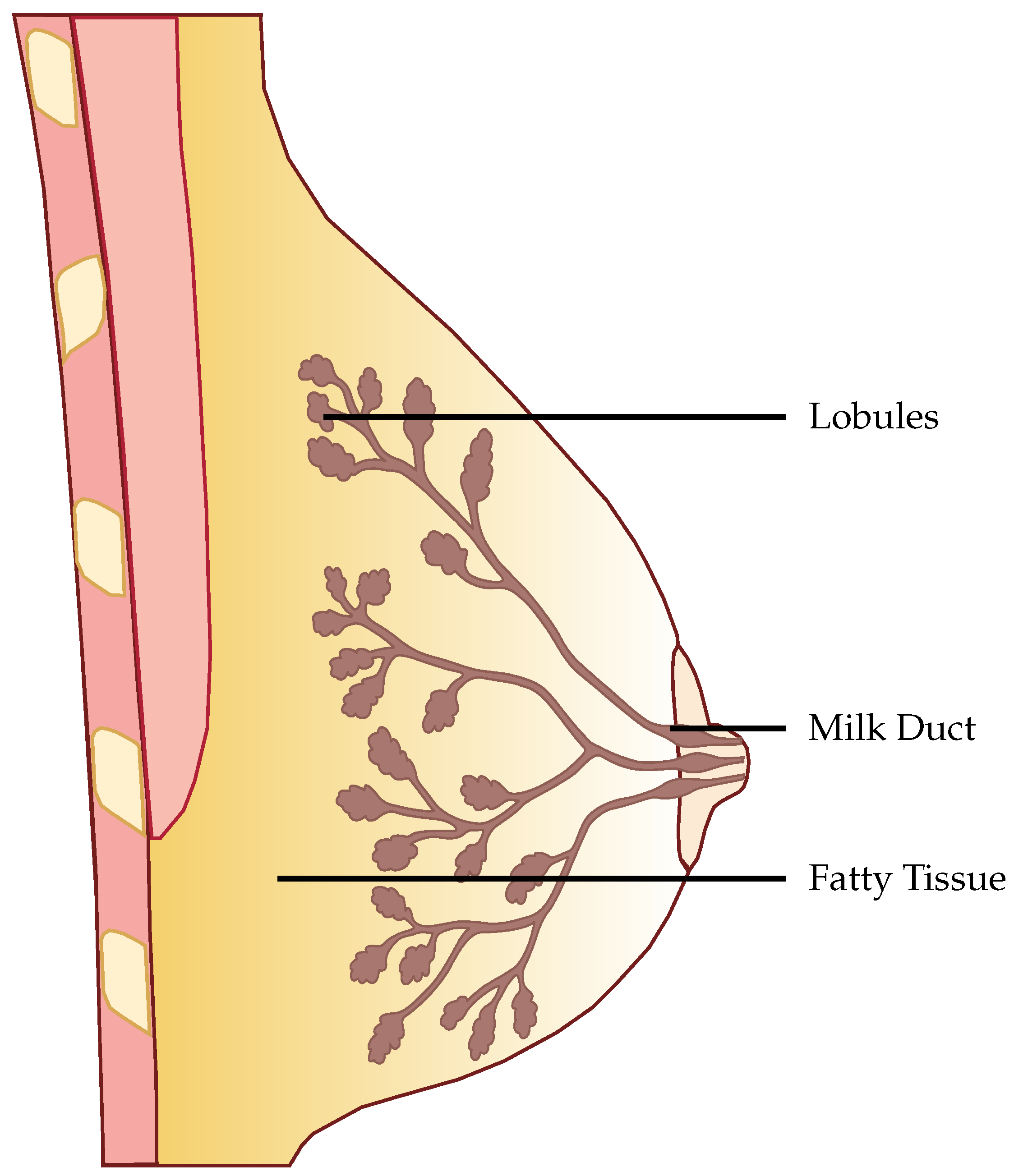
18]. EIDORS is a community-driven software package written in Matlab for FEM simulation in an EIT setting. The structure of the anatomical female breast is illustrated in Figure 1. In 
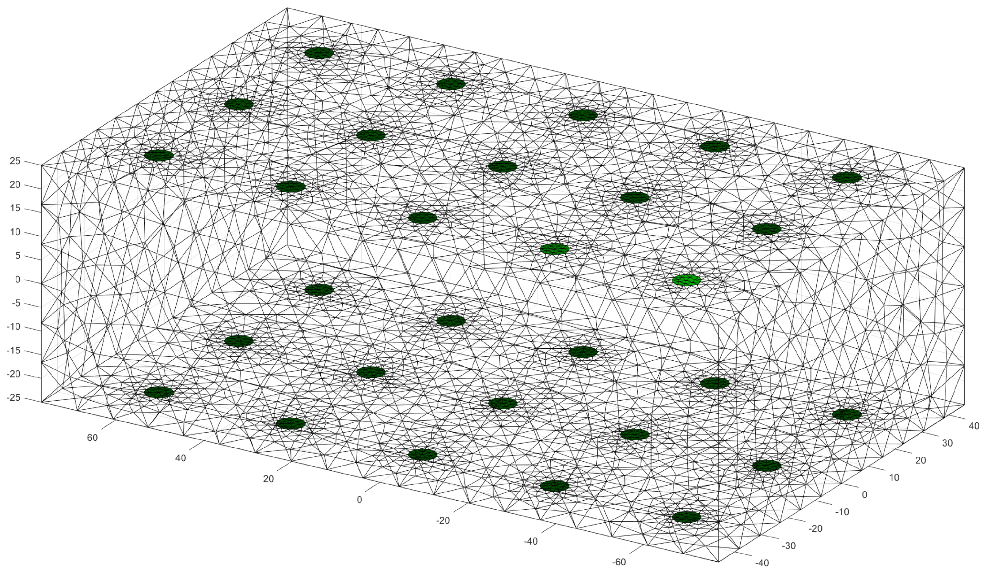
Figure 2 the used FEM model can be seen. The dimensions of the model are 50 m m × 154 m m × 92 m m . The electrodes have a radius of 2.9 m m . Fifteen electrodes are placed on each side of the model, thus, a total of 30 electrodes are involved in the model. The mesh size of the model was set to 2 m m , as this allows for a trade-off between the spatial resolution of the model and computation time. To avoid overfitting, 7500 different models were created. Each realization of the model was constructed according to the following rules.
To simulate the contact between electrode and breast, the contact impedance
Z c o n t a c t = 25 k Ω ( 1 + λ c o n t a c t · n ) ,
where Z c o n t a c t is the contact impedance, λ c o n t a c t is a weighting factor which, weights the contribution of the random sampling and n is sampled from a normal distribution N ( 0 , 1 ) . λ c o n t a c t was set to 1. This allows for modeling the variety in contact impedance.
We incorporated four different tissues into the model. On 5 sides of the model, a 2 m m thick layer of skin was introduced.
The glandular tissue was positioned within the domain, forming a truncated cone. The wider end of the cone was placed on the side without skin tissue and tapered towards the opposite end. This provided boundaries for the placement of the gland lobes. Within the cone, the lobes were placed randomly. Due to the inability to measure individual lobes, they were approximated as larger lobes [19]. These larger lobes had radii in all three spatial axes r sampled from a normal distribution N ( 3 , 0.513 ) with 1.46 m m r 4.64 m m , as reported in [19]. The orientation of these larger lobes was determined randomly by sampling all three Euler angles from 0 to 2 π 
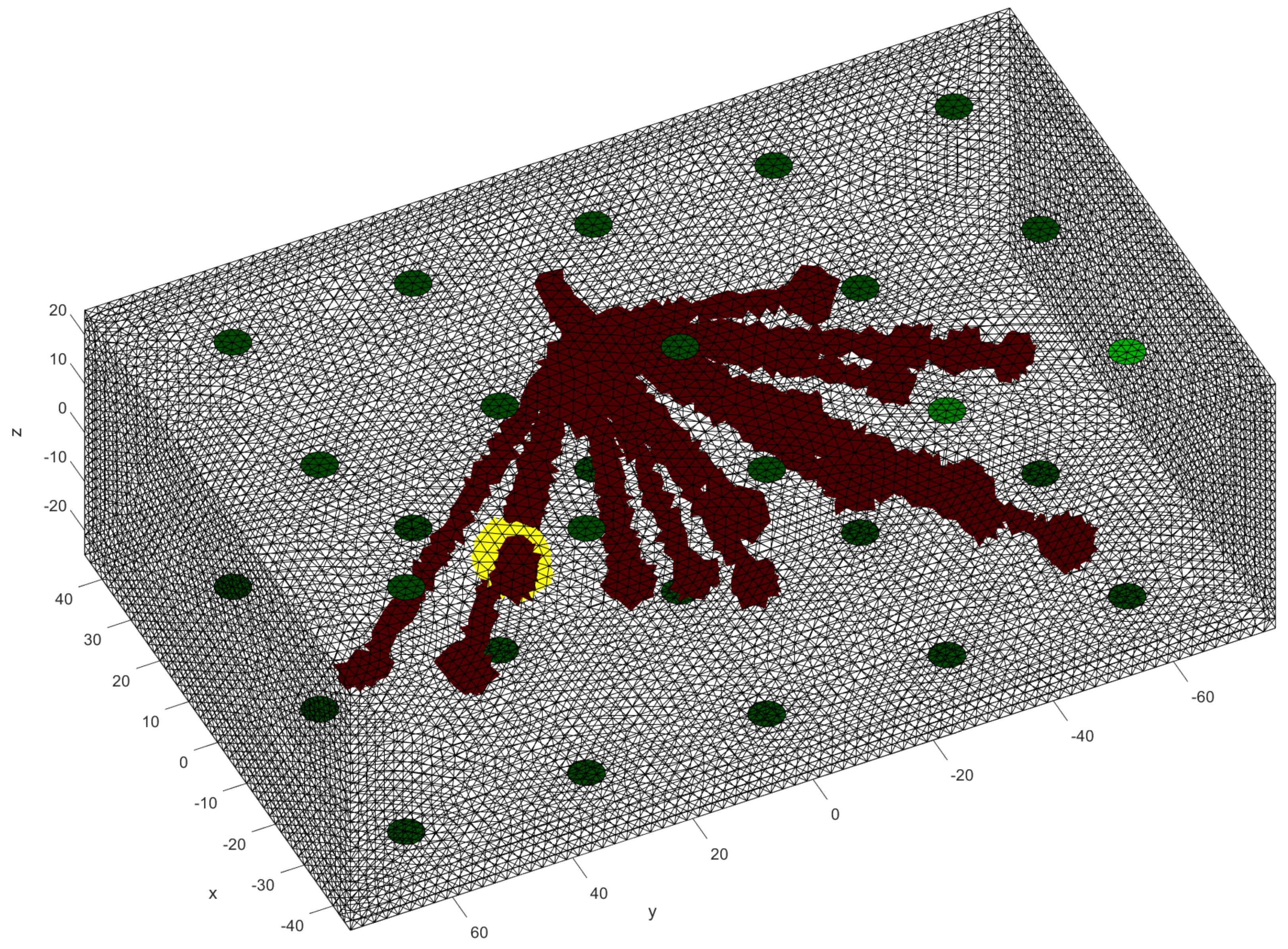
. A total of 20 larger lobes were positioned within the domain. From these larger lobes, a chain of ellipsoids or spheres with a radius of 1.5 m m extended towards the center of the truncated cone, as shown in Figure 3.
Just like big lobes in the glandular structure, the tumors are not perfect spheres and are distorted in all three spatial directions. The radii followed a normal distribution with the mean depending on the dataset created and a fixed standard deviation of 1 m m . We analyzed different mean values of radii from 6 m m up to 13 m m . The tumor was placed randomly, however, it was guaranteed that they always had contact with the glandular structure. An example of a tumor placement can be found in Figure 3, where the tumor is marked in yellow. Space that is not filled with any other tissue is assigned to fatty tissue.
The values for the conductivities of skin, fat, tumor, and glandular tissue are sampled as follows. In the literature, the values of all these tissue types are not fixed and have variations. For skin, the biggest conductivity value found is 2.93 × 10 3 S / m , the minimum value is 205 × 10 6 S / m , while the mean is 1.56 × 10 3 S / m [20]. Fatty tissue ranges from 12 × 10 3 S / m to 112 × 10 3 S / m with a mean of 52 × 10 3 S / m [12]. Glandular tissue ranges from 524 × 10 3 to 537 × 10 3 S / m with a mean of 530 × 10 3 S / m [21]. The conductivities were sampled such that they follow a normal distribution with a mean value given by the literature and a standard deviation σ , such that the 3 σ -interval lies within the minimum and maximum range. After a value is sampled, each mesh element is varied 5 % around the value, to model inhomogeneities inside the tissue [20].
The injection-measurement pattern was set to adjacent-adjacent for each electrode plane. In our set-up, we have 3 planes of 10 electrodes each.
When the voltages were simulated, white Gaussian noise was added to the voltages with the help of the EIDORS function add_noise(). The magnitude of the noise was set regarding the characteristics of the dataset.
From this general structure of the data set, we can vary the following attributes:
  • Noise of the voltages
  • average size of the included tumors
In Section 3, we give the parameters for all performed analyses. Note that every data set had a 50/50 split of healthy and carcinogenic breast tissue. Furthermore, we note that this was done on purpose, to provide a balanced dataset for proper training. If we had a data set containing a realistic proportion of tumors, the models would get good results by simply guessing non-tumor every time.

2.2. Choice of Models

We have chosen RF, SVM and ANN as the basic models for our comparison, each with different underlying principles. SVMs, as linear models, define a boundary through linear algebra, while RFs, as ensemble learning models, generate multiple decision trees during training and combine these decisions to make predictions, providing valuable insight into the origins of their output. On the other hand, ANNs, due to their non-linear nature, are able to capture intricate relationships between data points, potentially offering superior performance in dealing with the inherently ill-posed and non-linear problem of identifying conductive enclosures, particularly tumours in our context. Detailed explanations of these models are given in the following sections.

2.3. Random Forests

The RF model is based on an ensemble of single decision trees first developed by Breiman [22]. A decision tree is a type of model used for classification and regression. It operates by using the values of the input features to recursively partition the data into subsets. For every division, select the feature that divides the data most effectively. The tree continues to grow until all the data in a subset belong to the same class, or until a stopping criterion has been met. The final tree can be used to classify new data by following the splits from the root to a leaf node. The class label is assigned to the leaf node. The subdivisions in a decision tree are chosen to maximize the reduction in impurity. Either Gini impurity or entropy is commonly used to measure this reduction in impurity based on the training data. The impurity gives insight into the separability of the data. For more information about the Gini impurity and entropy in RFs, we recommend the PhD thesis from Gilles [23]. If only one decision tree is used, the process is prone to overfitting, as it will be specifically fit to the dataset. To tackle this issue, an ensemble of decision trees called random forest is used.
For the implementation of the model, we used the scikitlearn-library [24].
For a given dataset, the hyperparameters of RFs were optimized through grid search. The inputs to the RF classifier wee:
1.
n_estimators: number of trees in the forest varied from 15 to 350.
2.
max_features: number of features looked at for the best split (we tested “sqrt” and “log2”).
3.
max_depth: maximum depth of a single tree, varied from 15 to 150.
4.
bootstrap: the whole dataset used for a single tree, either “True” or “False”.

2.4. Support Vector Machines

SVMs take a different approach to classification, employing linear algebra to find a separation between the classes. This is done by fitting a hyperplane that best separates the clusters, such that the margin between the closest data point from each class and the hyperplane is maximized. These closest points are called support vectors. If a direct separation in the dimensionality of the data is not possible, the data is transformed to a higher dimension, where the fitting is carried out. This is done through the kernel-trick. A commonly used kernel is the radial basis function (RBF) kernel [25].
We also used the scikitlearn-library for the implementation of the model [24].
Just like in the case of RFs, for SVMs we also performed a grid search for the optimal parameters for a given data set. As a kernel, we used the RBF kernel. We performed a grid search on the following inputs to determine the best-performing SVM:
1.
C: regularization parameter for the L 2 -regularization.
2.
gamma: controls the shape of the decision boundary.

2.5. Artificial Neural Networks

ANNs model the structure of our brain, in order to approximate (non-linear) functions. They consist of synapses that have multiple inputs and multiple outputs, the inputs are connected through a linear function and is made non-linear through a non-linear activation function. The synapses are modeled as matrix multiplications with the input, while the result is fed through an activation. The training is done in a supervised manner, which means that the input data and the appropriate output data is provided during training. The parameters of the ANN are then altered such that they maximize the user-specified loss function.
For the implementation of our ANN, we used Keras Tensorflow [26].
In our case, the implemented ANN had nine fully connected layers, which decreased from 680 neurons in the first layer down to 15 in the last hidden layer. For all but the last layer, Rectified Linear Units (ReLUs) were used as activation functions. The last layer used sigmoid as an activation function to bind the classification between 0 and 1.

2.6. Evaluation Score

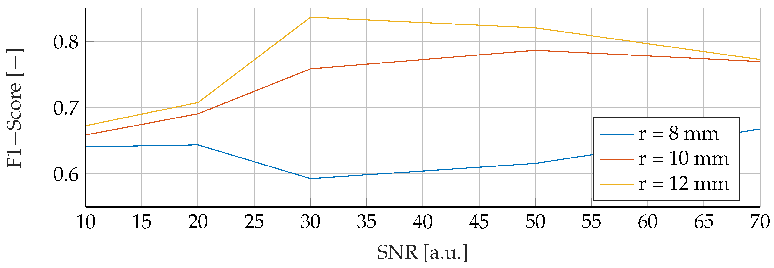
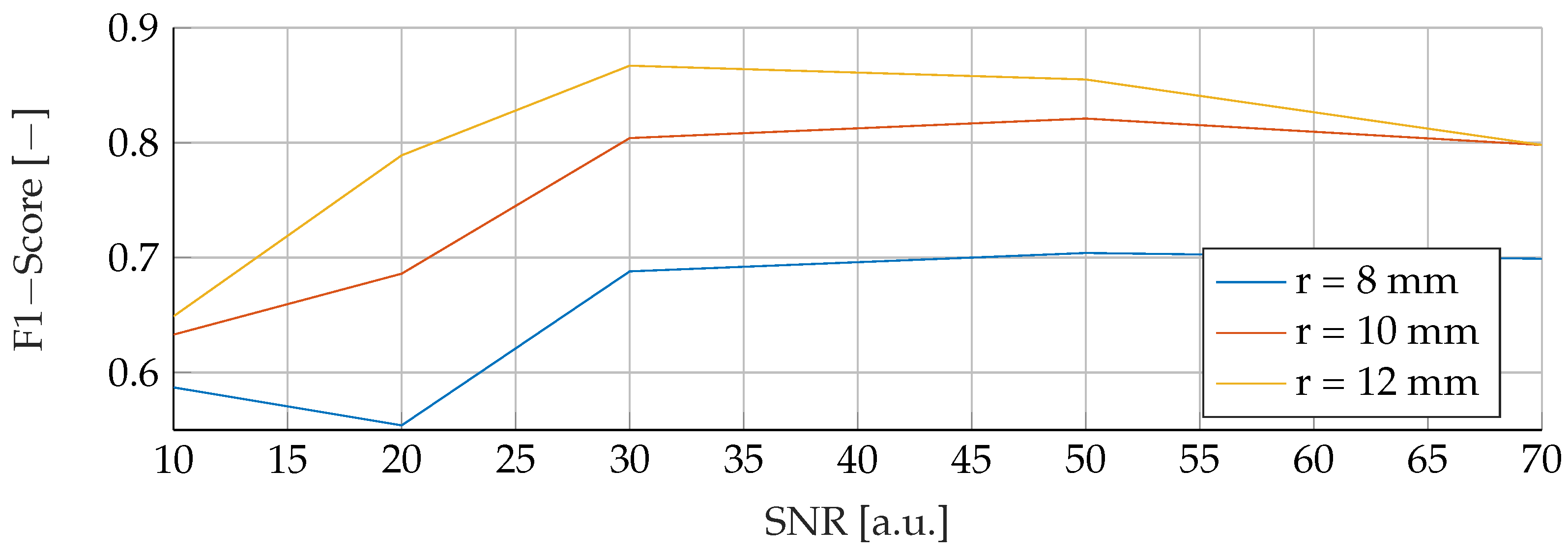
For the evaluation of the different models and data combinations, the F1-Score was chosen. In a real-world setting, it is utterly important to not miss any cases of breast cancer. Further, avoidance of false positives is also really important, as the patient might undergo unnecessary stress.
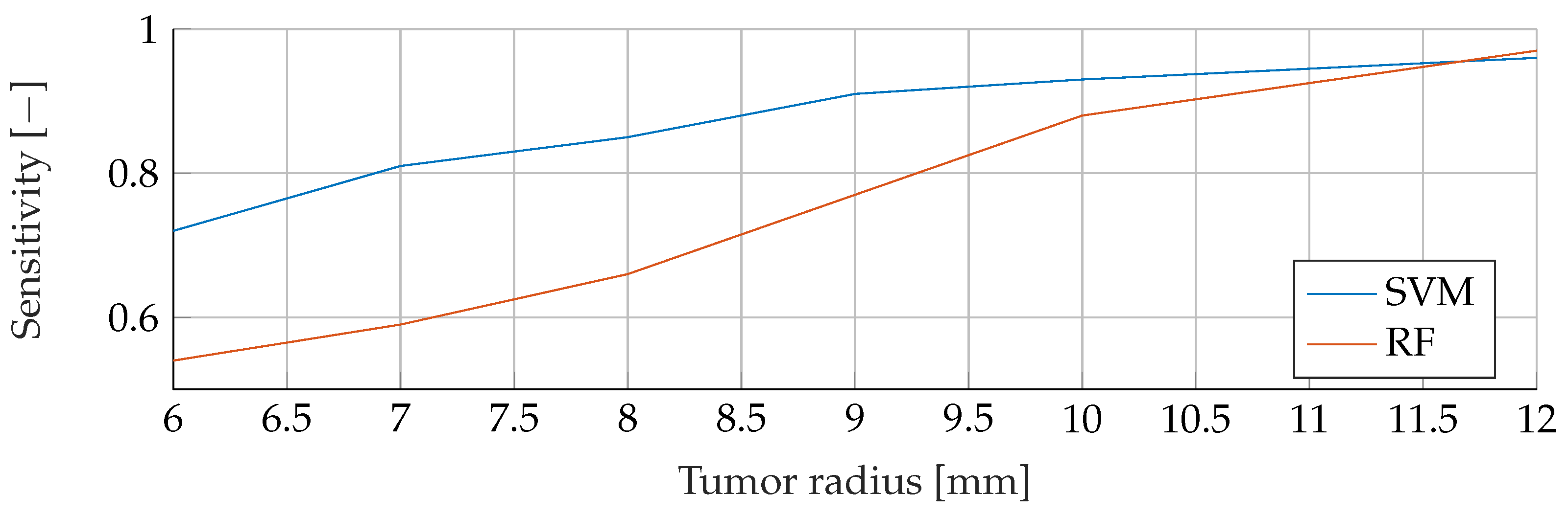
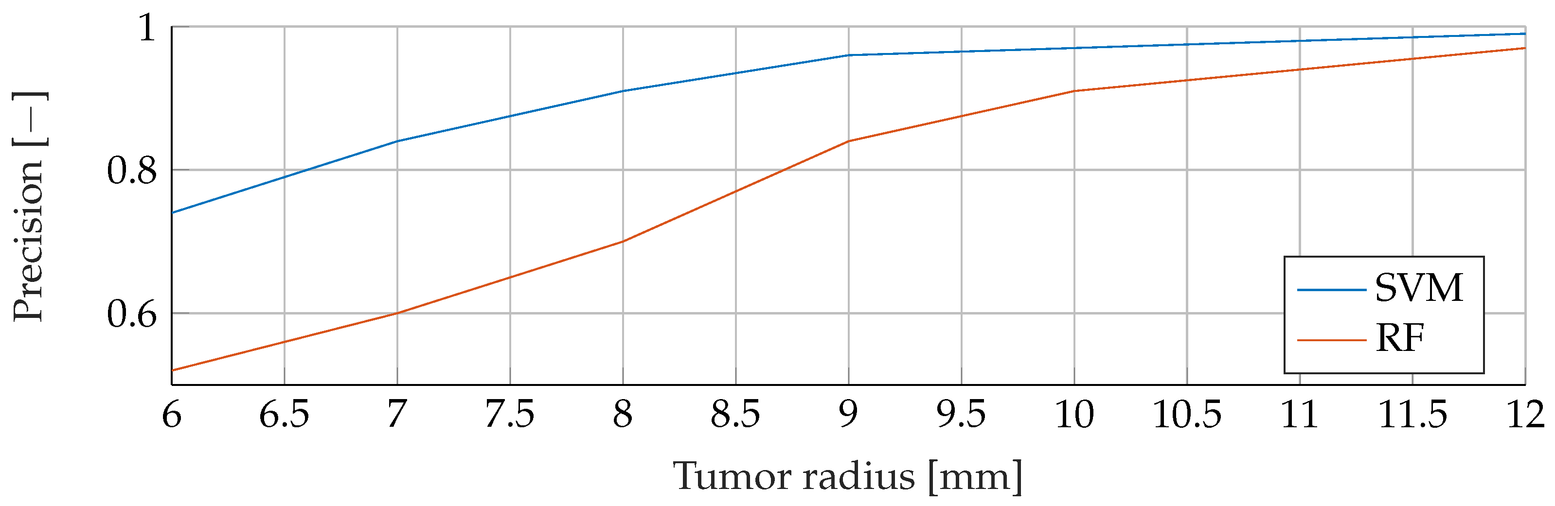
The F1-Score is calculated from 2 metrics [27]. First, the Precision, measures how many positive predictions by the model were correct. Second, the Sensitivity, which measures how many of the positive samples out of the dataset were correctly predicted. Thus, it takes into account wrongly identified as positive. Positive, in this case, means a tumor is present. The F1-Score takes not only into account how many tumors the model classified rightfully as a tumor, but also how many predictions were falsely identified as a tumor.
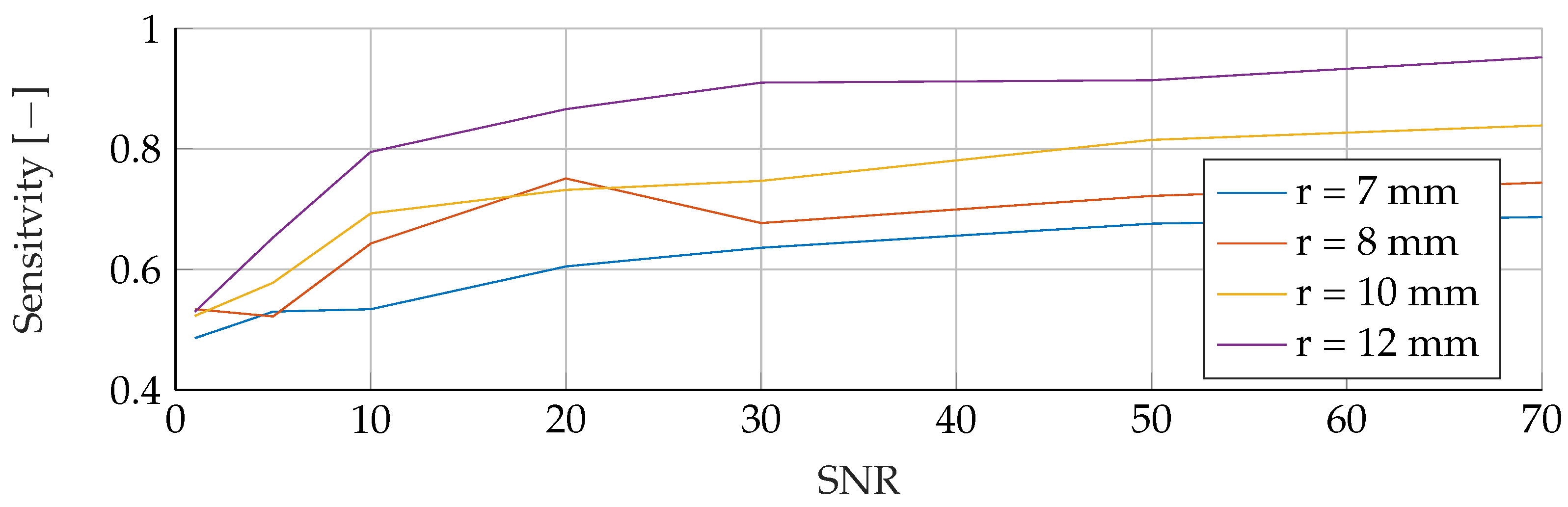
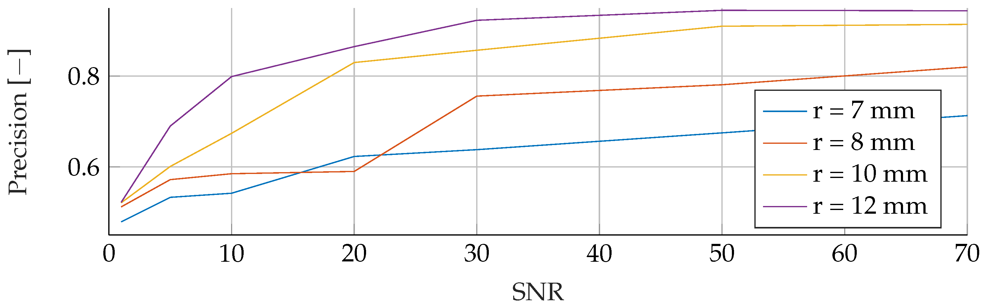
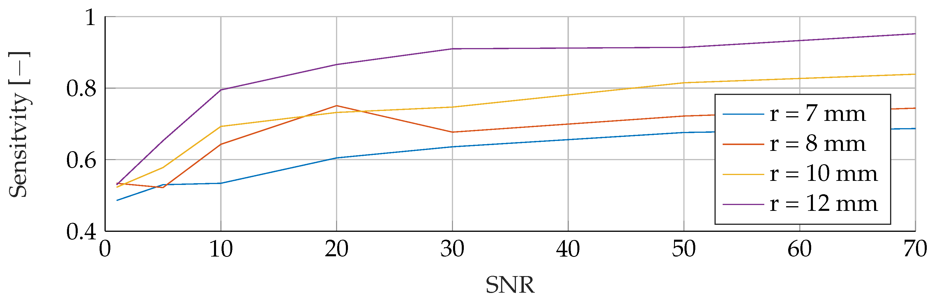
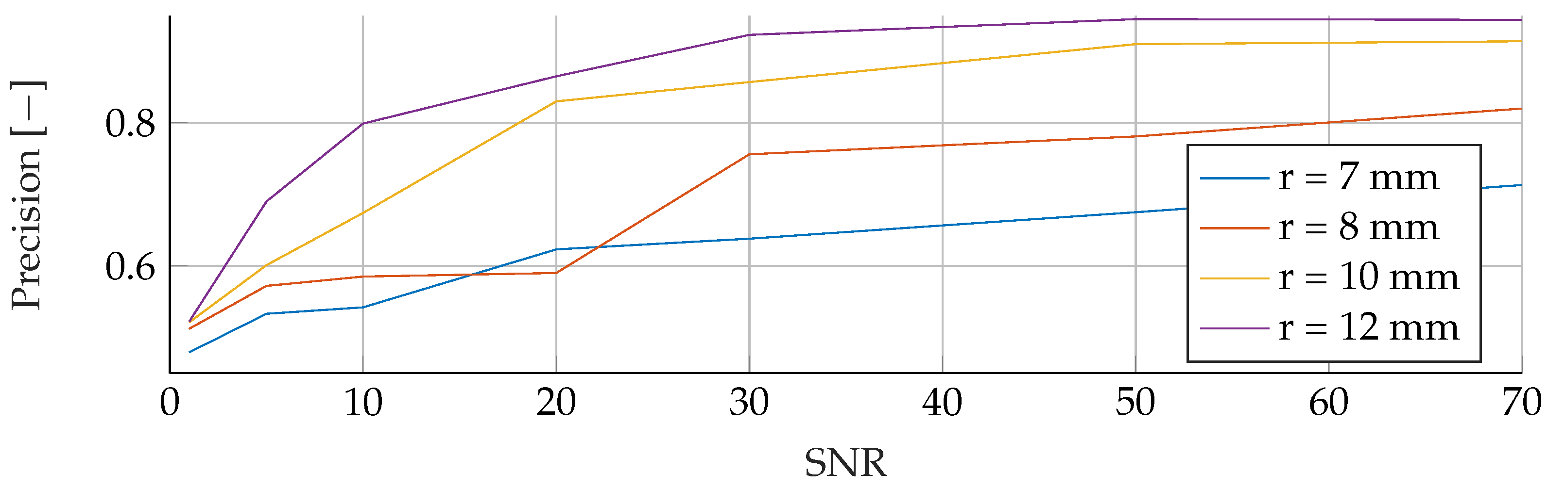
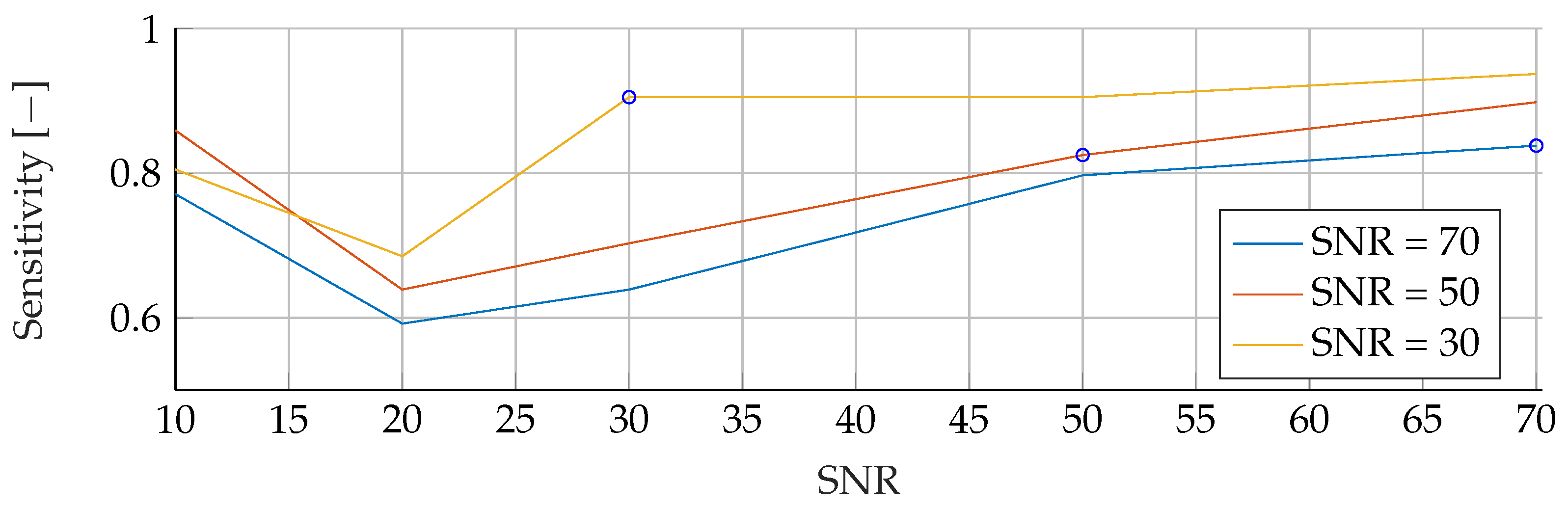
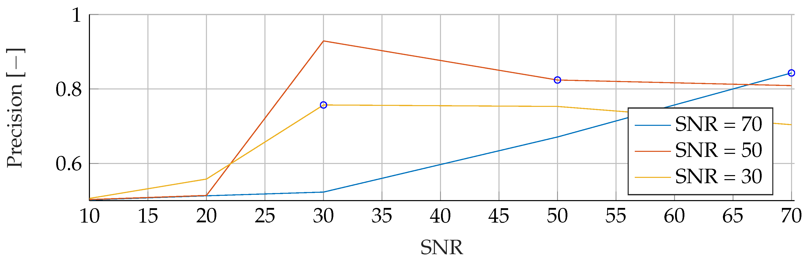
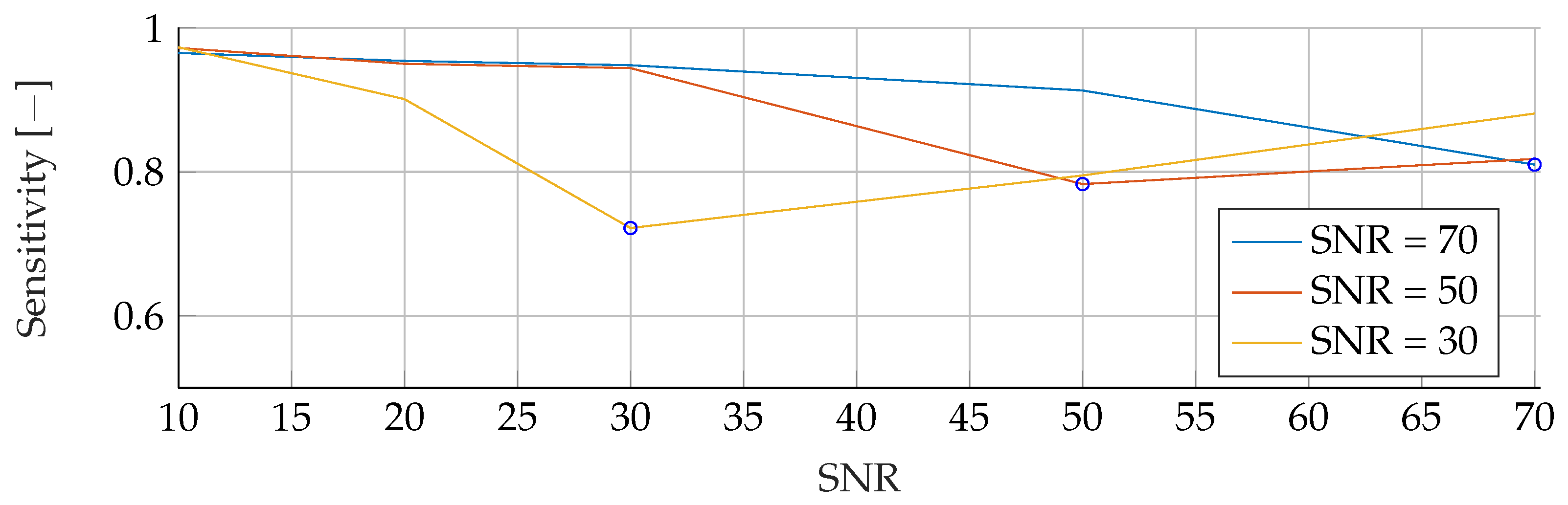
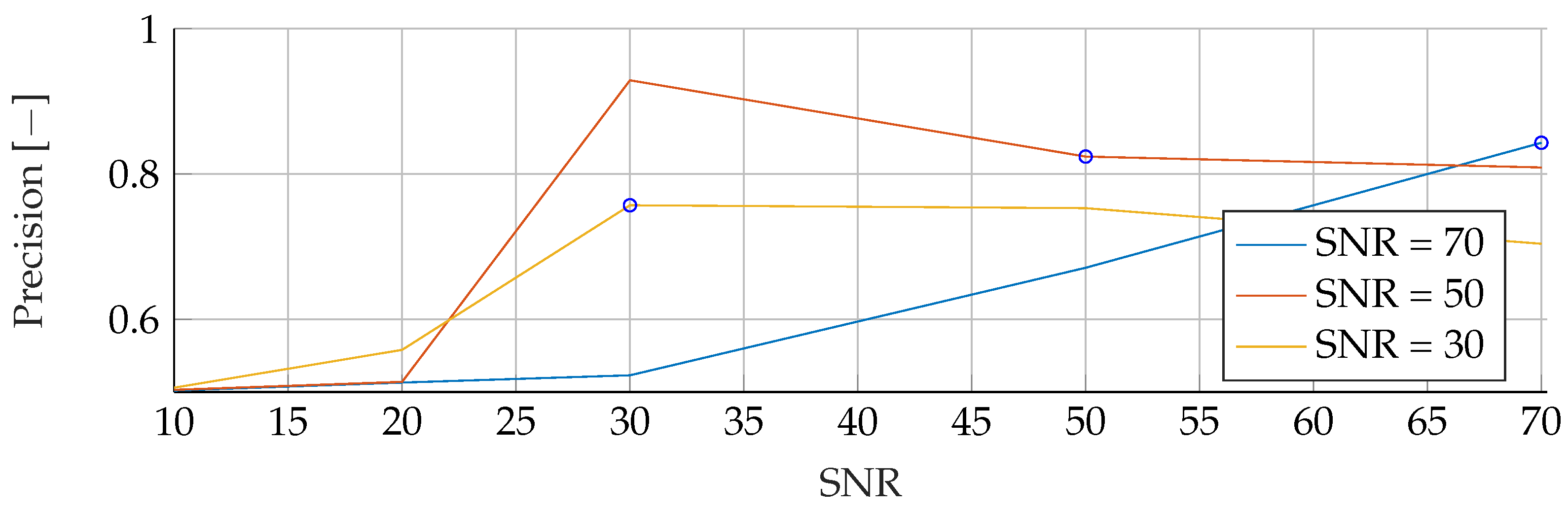
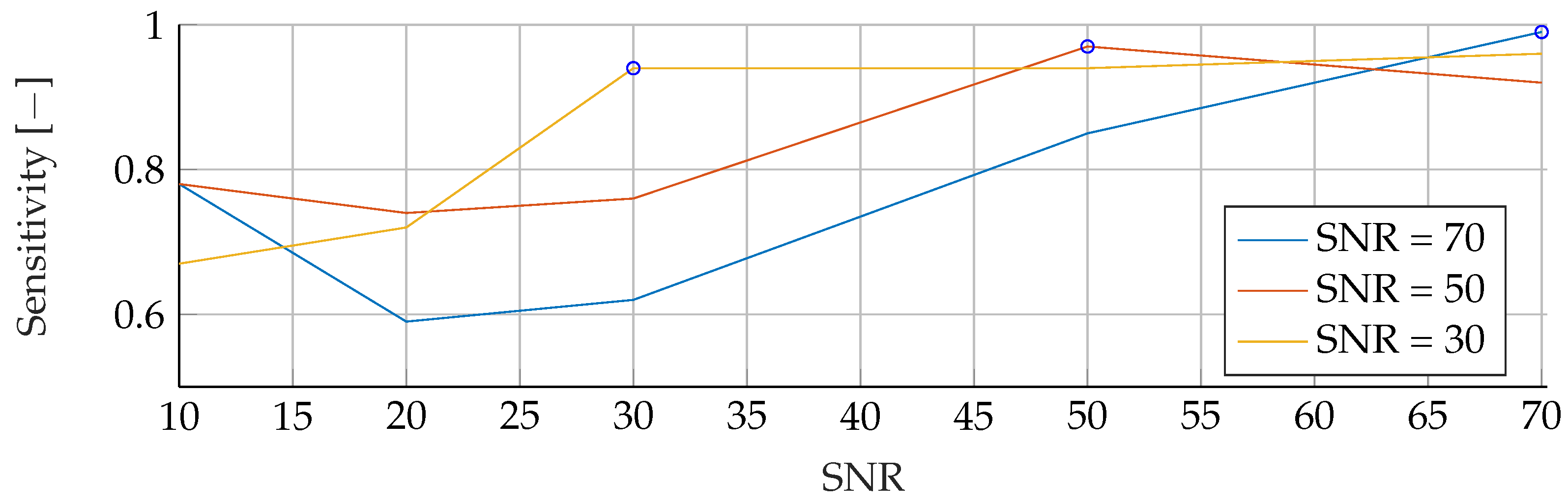
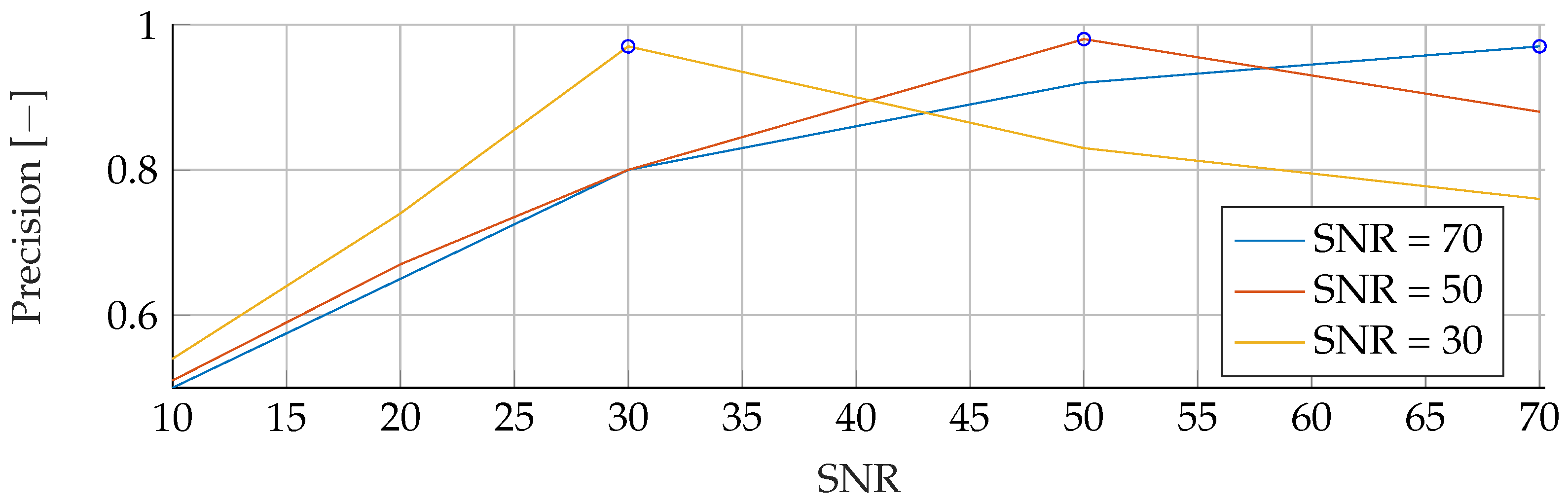
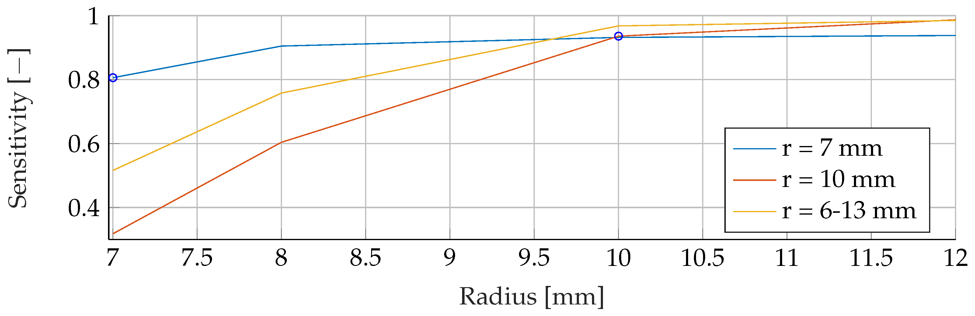
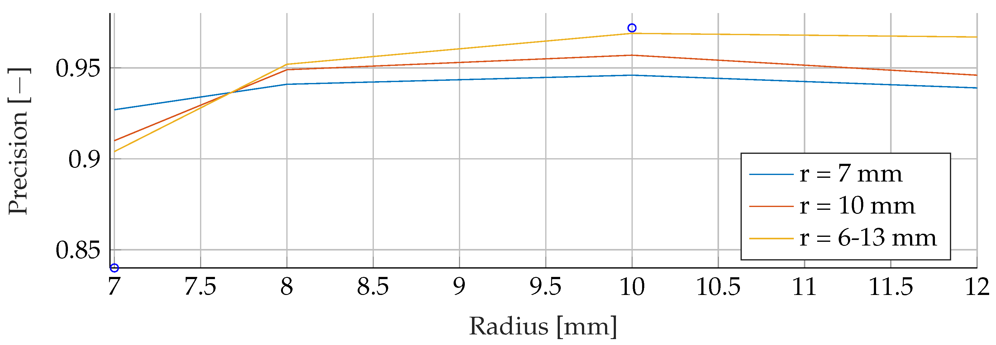
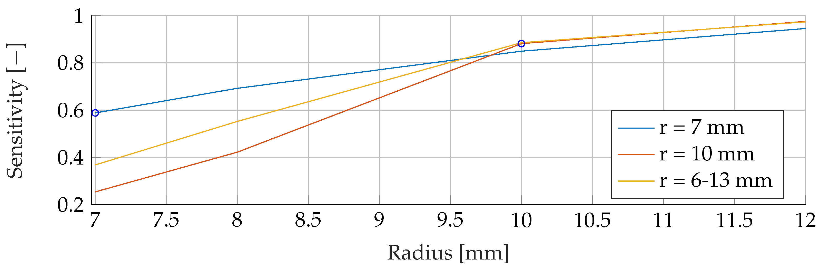
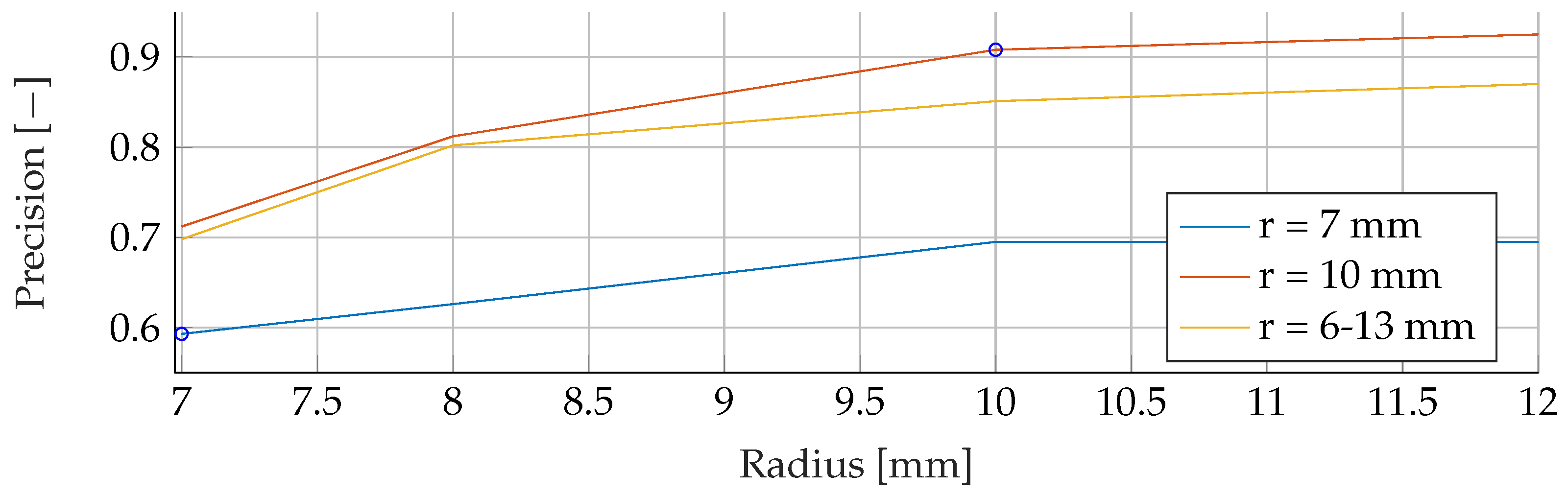
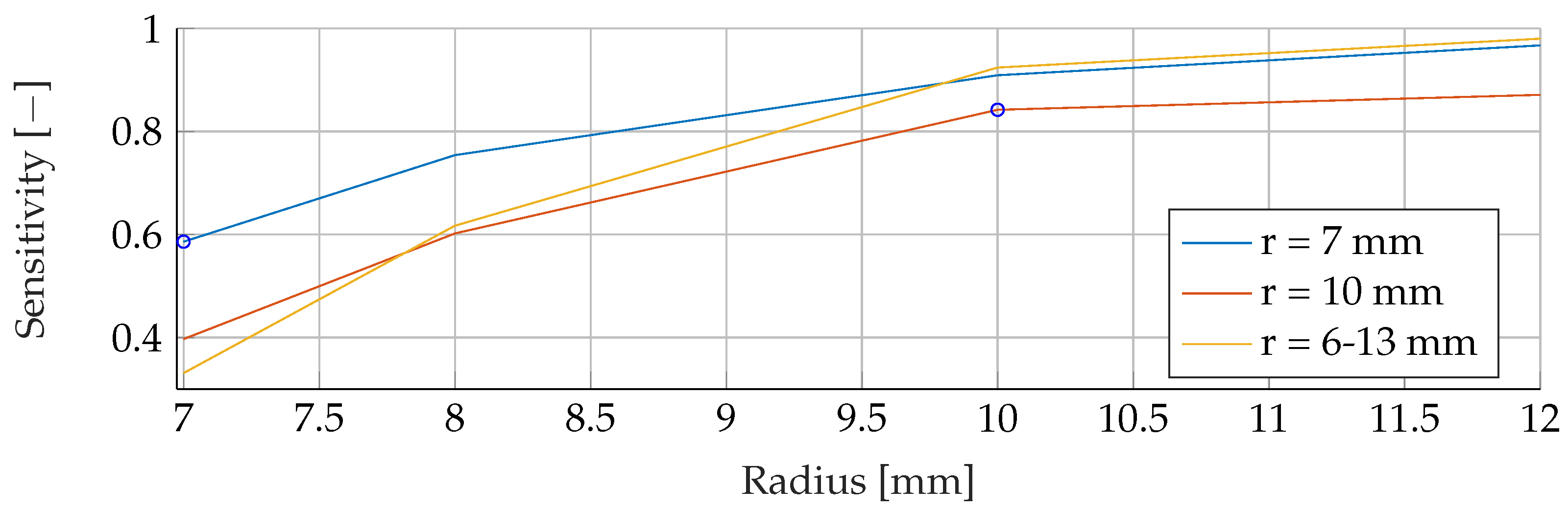
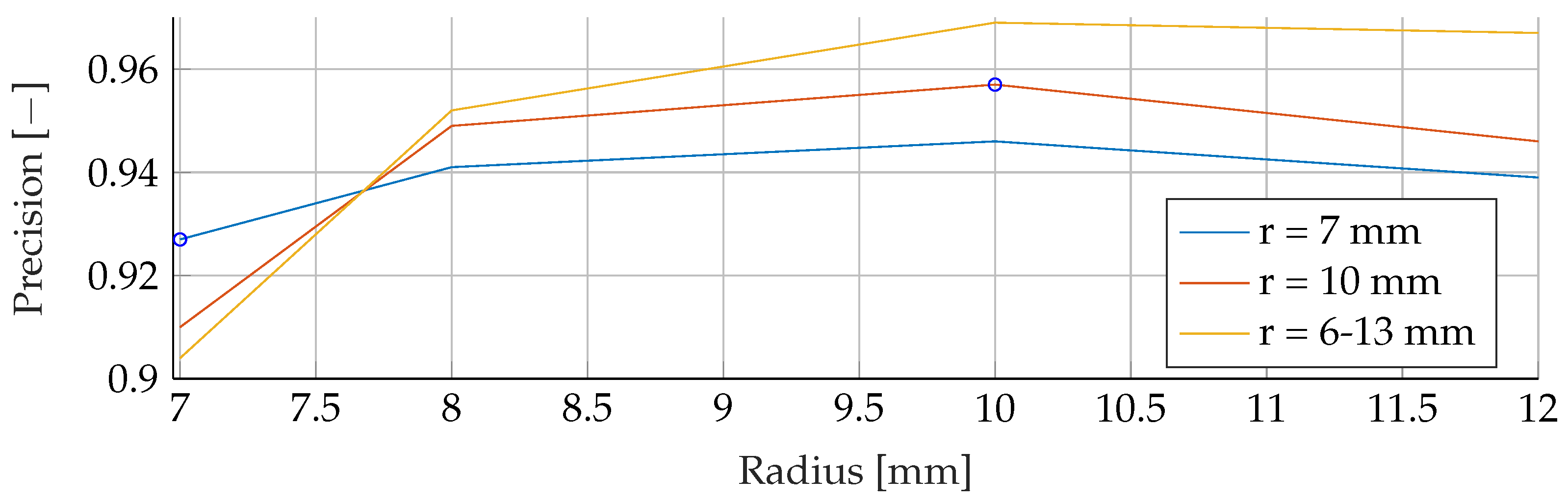
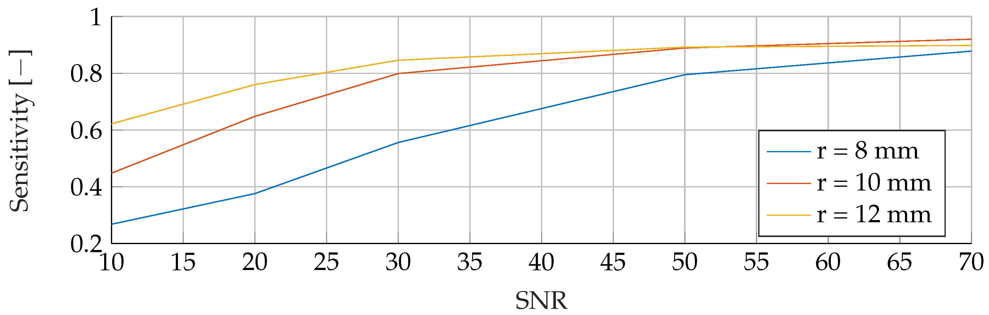
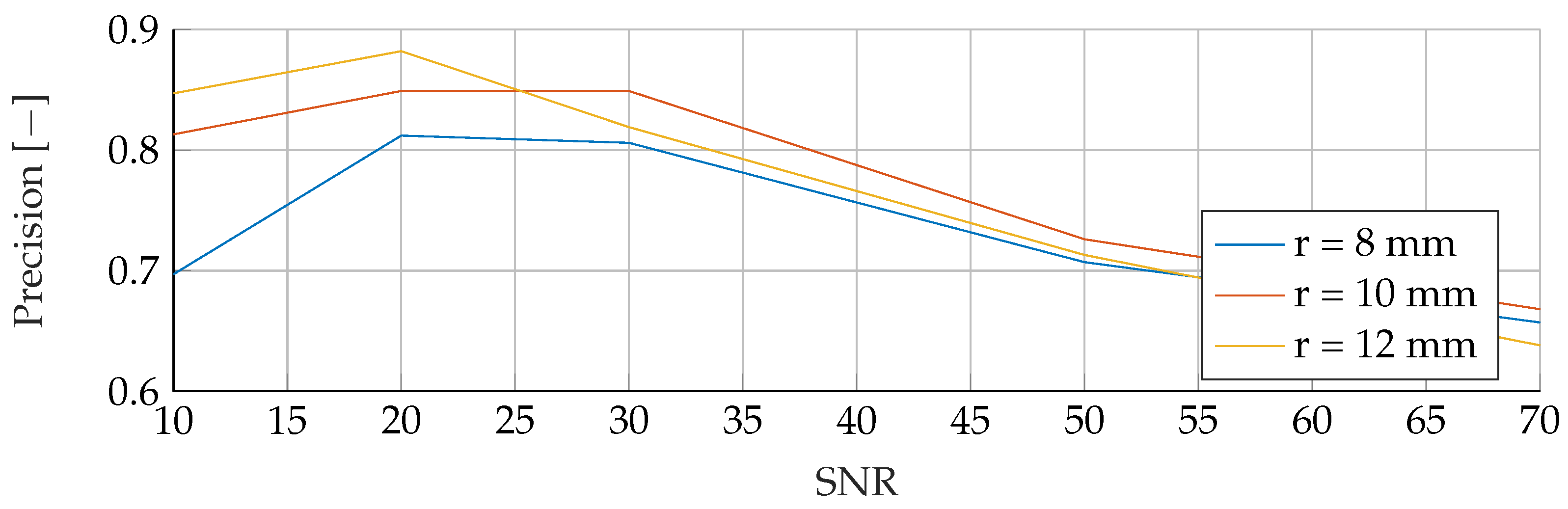
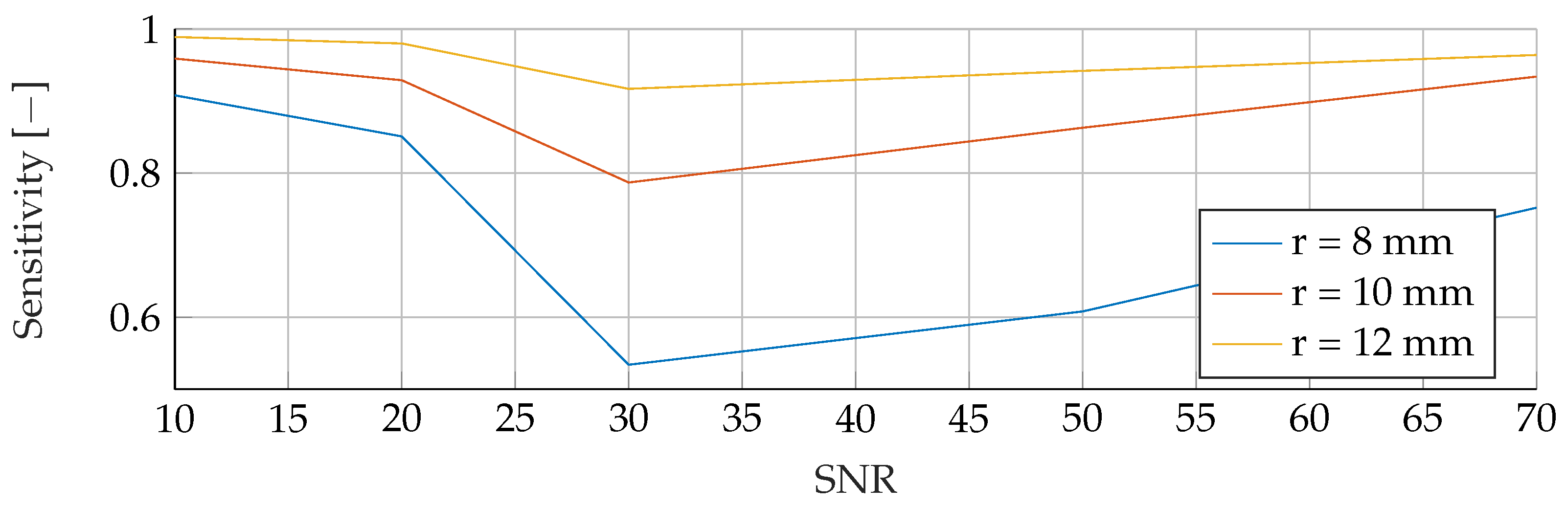
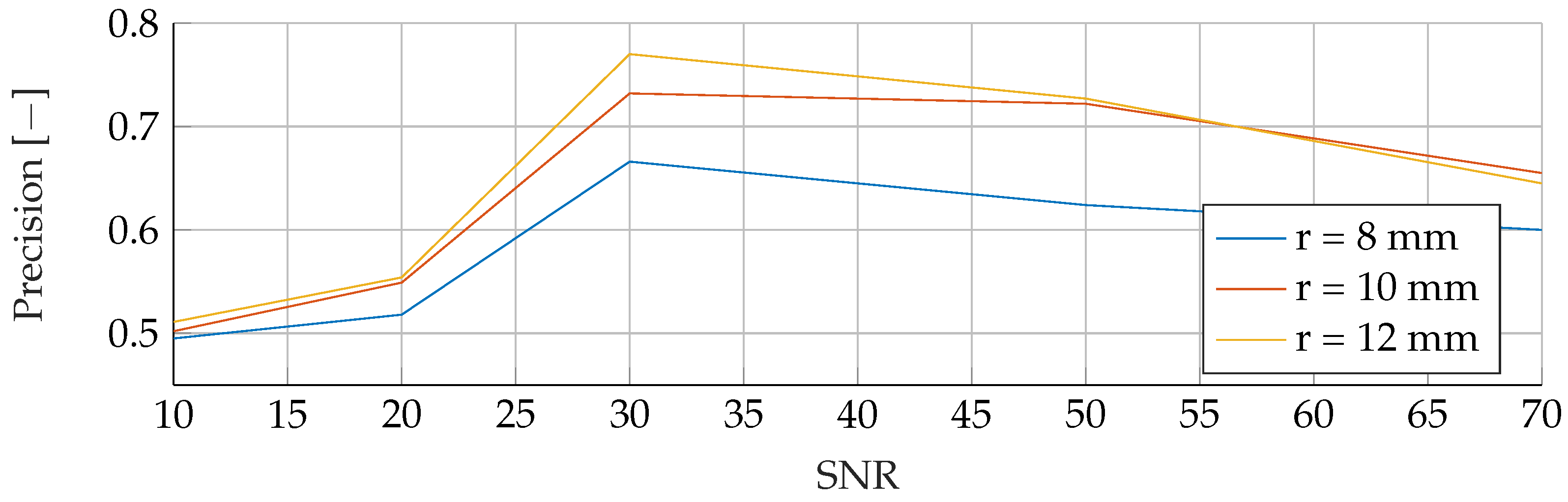
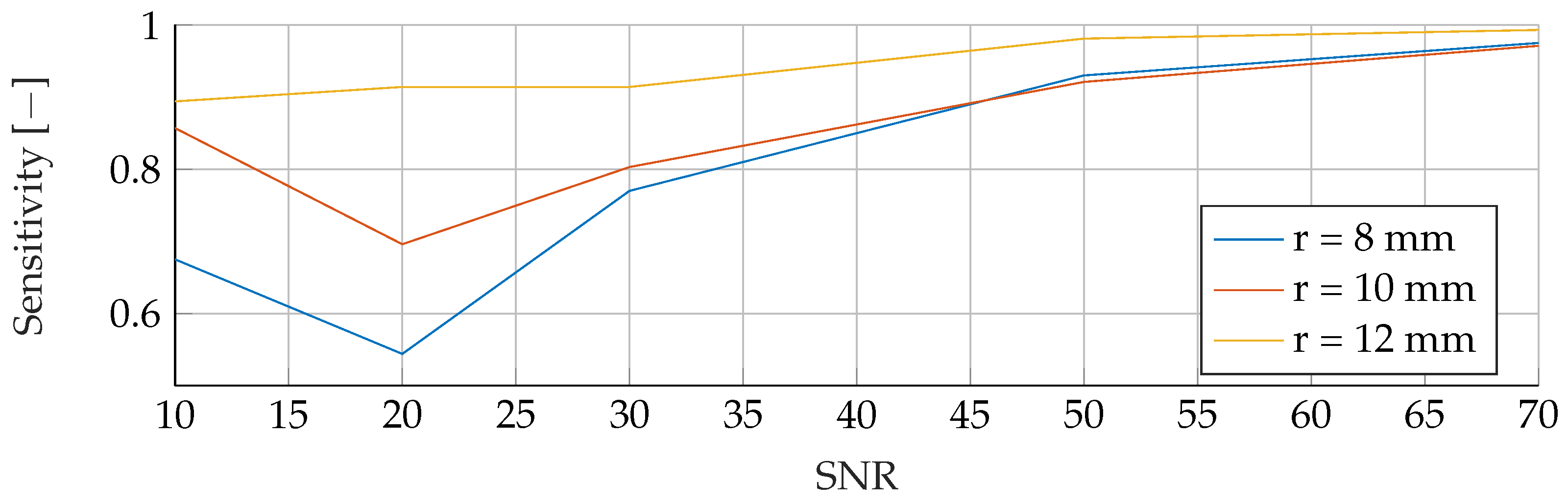
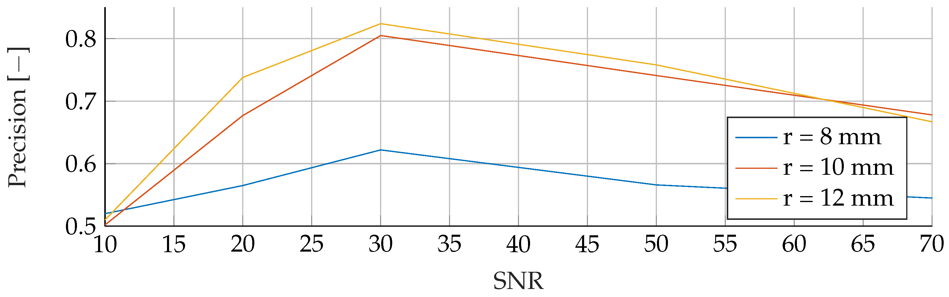
In the Appendix A, we have provided the Precision and Sensitivity for each figure in the results section of the paper. Readers who are interested in further understanding are kindly asked to see the Appendix A for further details. We have limited our analysis to the F1-Score, as it is useful for avoiding false positives in the real world. the second reason is that adding additional metrics would increase the length of the paper even further, as we provide combinatorial analysis for different noise setups and tumor radii.

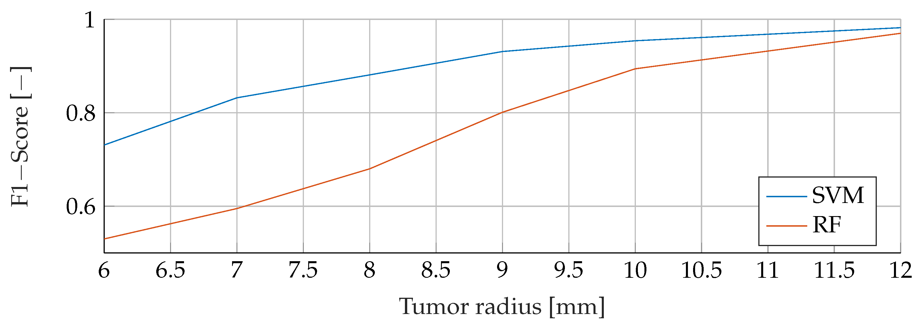
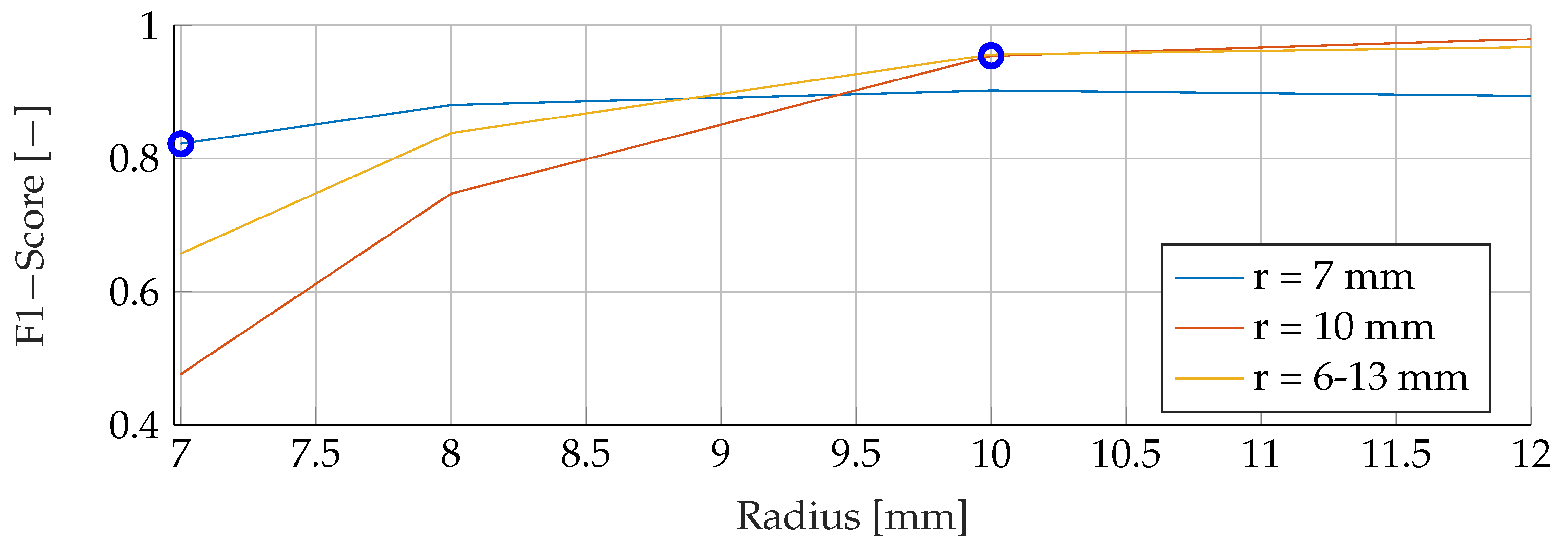
2.7. Evaluation Methodology

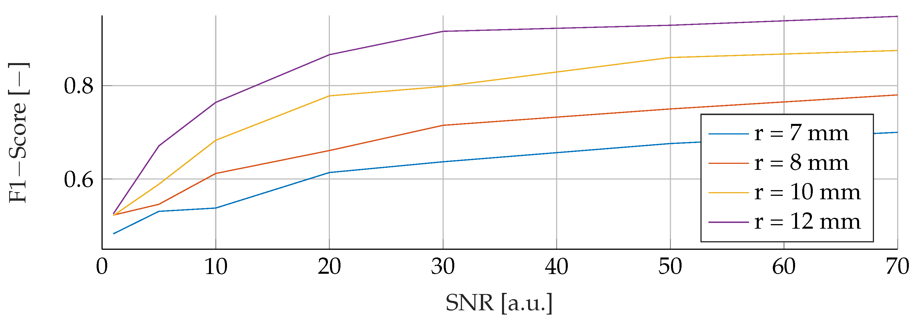
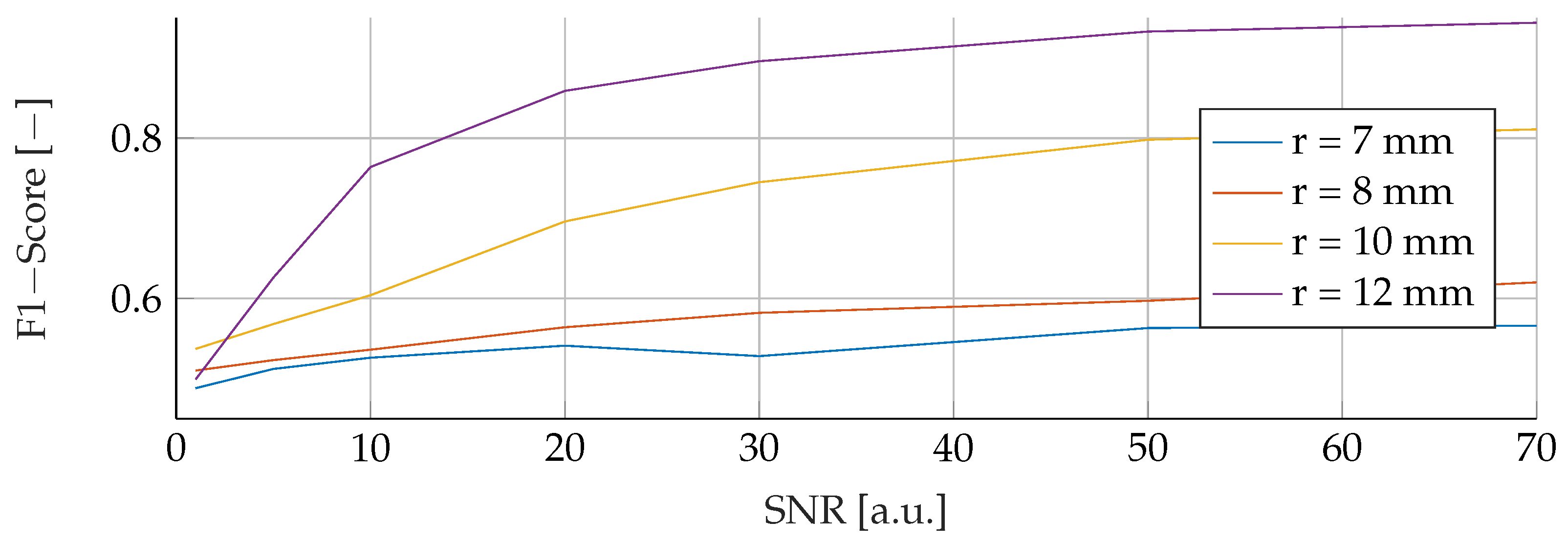
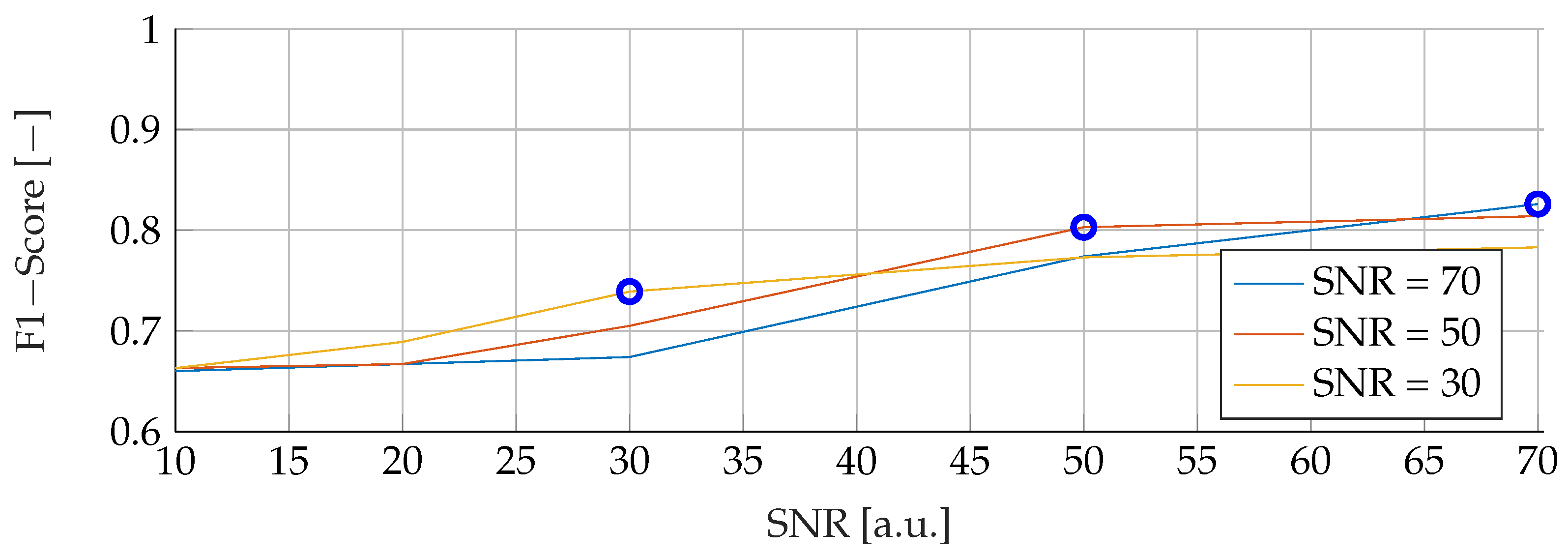
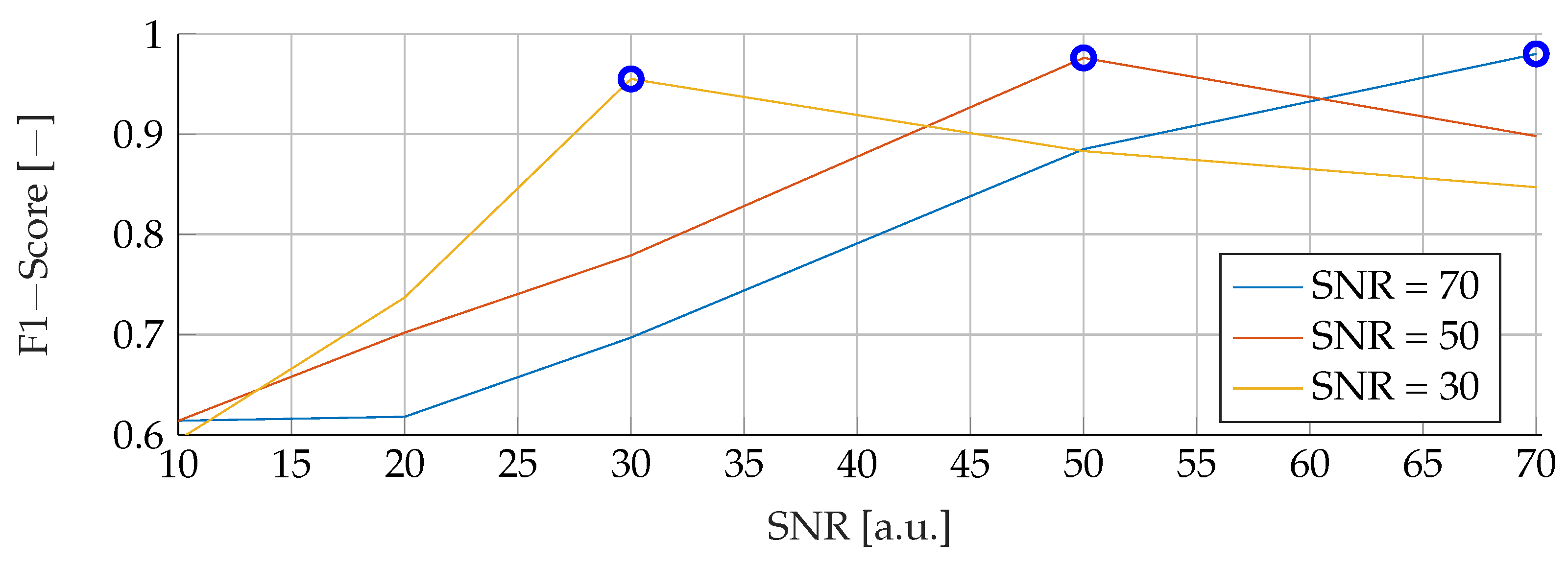
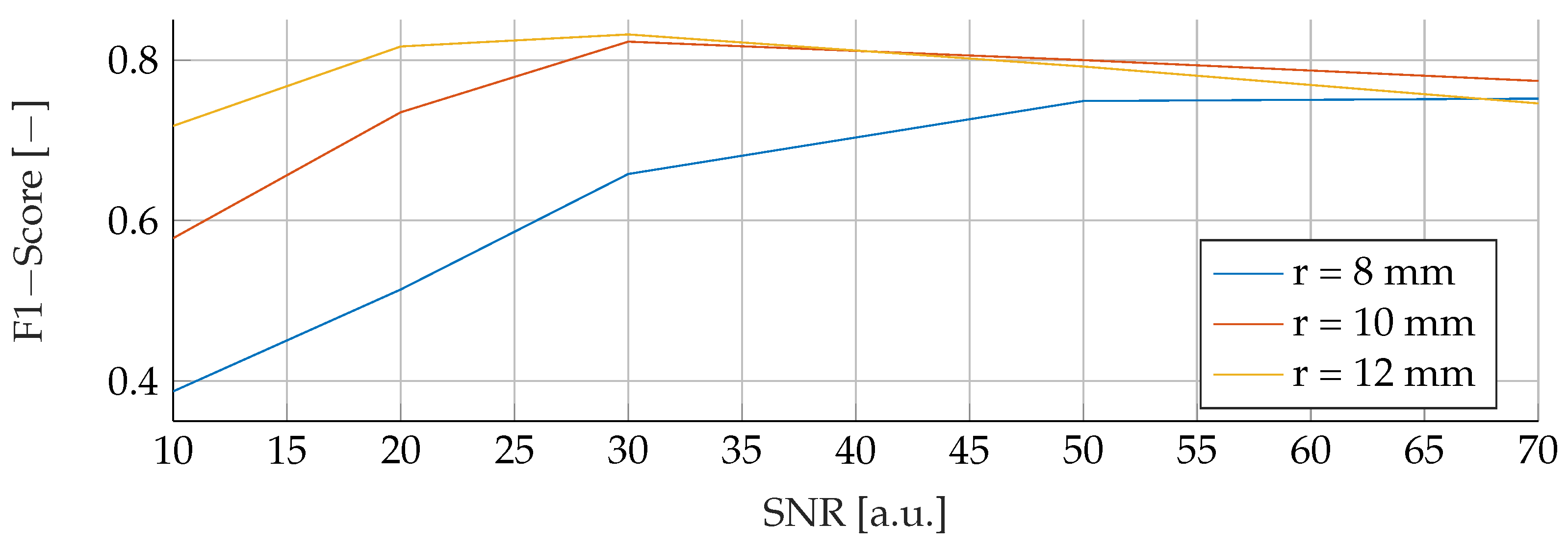
Our proposed models were subjected to a thorough evaluation process across a variety of carefully crafted simulated scenarios. We began by examining the models’ performance in noise-free conditions, focusing on the relationship between tumor radii variations and the resultant F1-Score. To mimic real-world conditions, we introduced noise at various signal-to-noise ratios (SNRs) and assessed the models’ robustness against these perturbations. We also evaluated the stability of the models by training them at specific SNRs and testing them under different noise levels, revealing valuable insights into their adaptability. Furthermore, we conducted an in-depth investigation into the models’ performance when trained with a wide range of mean tumor radii. Finally, we put the models to the test under stringent conditions involving a broad range of tumor radii and an SNR of 30. This rigorous evaluation process aimed to provide a detailed understanding of the models’ capabilities and constraints, thereby presenting a holistic view of their performance across diverse simulated scenarios.

3. Results

3.1. Noise-Free Basis Data

To conduct an initial analysis, we undertook a comparative study of the Support Vector Machine (SVM) and Random Forest (RF) models. Our investigation utilized a meticulously curated dataset, featuring samples devoid of noise and encompassing tumor radii spanning the range of 6 m m to 12 m m . This preliminary assessment aimed to verify the integrity of the data and validate the robustness of our approach. The outcomes of this evaluation, illustrated in Figure 4, unveiled a notable trend: as the tumor radius increased, the F1-Score exhibited a corresponding upward trajectory. Specifically, when considering a tumor radius of 6 m m , the RF model yielded an F1-Score of 0.52, while for a radius of 12 m m , this score ascended to 0.97 . In comparison, the SVM model achieved an F1-Score of 0.73 for a 6 m m radius, which soared to 0.98 for a 12 m m radius. Consequently, it became apparent that as the tumor size expanded, the discernible disparities between the performances of the SVM and RF models diminished.

3.2. Noisy Basis Data

In the subsequent analysis, we delved into a comprehensive comparison between SVM and RF under the influence of noisy training data spanning the spectrum from 7 m m to 12 m m . Throughout this investigation, the noise levels were carefully manipulated, varying between an SNR of 0 and 70, while maintaining consistent test conditions for each corresponding noise level and tumor radius. Figure 5 vividly illustrates the SVM model’s performance nuances amidst fluctuations in noise and tumor radius, while Figure 6 similarly shows the subtle response of the RF model under the same varying conditions. Notably, both figures exhibit a strikingly similar pattern across all curves. A notable trend in the results is the inverse relationship between F1 score and SNR. This trend is further reflected in relation to the tumor radius, showing that as the SNR decreases, the F1-Score decreases proportionally. For example, for a tumor radius of 7 m m and 8 m m , the F1-Score for the RF model escalates from 0.48 to 0.56 and 0.51 to 0.62 , respectively, with increasing SNR. In contrast, the F1-Score for the SVM experiences a larger increase, rising from 0.48 to 0.7 and 0.52 to 0.78 , respectively, for the corresponding radii. The peak performance for both the SVM and RF models was achieved at the highest levels of SNR and tumor radius, culminating in an F1 score of 0.94 for both models.

3.3. Stability under Different Noise Levels

Our subsequent analysis focused on analyzing the noise stability of the SVM, RF and ANN models. Each model was meticulously trained on noisy data at varying SNRs of 30, 50 and 70, followed by testing with noise levels ranging from 10 to 70. The resulting data is visually illustrated in Figure 7, Figure 8 and Figure 9 for SVM, RBF and ANN, respectively. For all models, it is apparent that lower SNRs during testing, compared to the SNR during training, lead to a significant reduction in the corresponding F1-Score. Notably, the F1 score showed a consistent downward trend as the SNR decreased. In particular, during training with an SNR of 30, the SVM model reached its peak performance when tested with the same noise level in the test data. Deviations from this optimal SNR resulted in a subsequent decrease in the F1 score. Meanwhile, at an SNR of 50, the SVM model showed a slight increase in F1-Score when applied to higher SNRs, reaching values of 0.85 and 0.87 , respectively. However, training datasets with an SNR of 70 showed a deterioration in F1-Score when subjected to higher noise levels, dropping from its peak value of 0.87 . Conversely, the RF model performed consistently better at higher SNRs, regardless of the level of noise present in the training data. Despite minor variations, the F1 scores remained closely distributed, with a maximum deviation of 0.07 However, it is worth noting that the overall F1 scores for the RF model were relatively lower compared to the other models considered. In contrast, the ANN model proved to be highly sensitive to any deviations in the unseen data, despite showing the highest overall scores of all the models. An increase or decrease in the trained SNR resulted in a substantial decrease in the F1 score. Specifically, when the SNR of the test and training data were equivalent, F1 scores of 0.95 , 0.97 , and 0.98 were found for training data noise levels of 30, 50, and 70, respectively.

3.4. Stability under Different Tumor Radii

This section provides a comprehensive analysis of the results obtained for different tumor radii. The models were trained using mean tumor radii of 7 m m and 10 m m , with a wide range of tumor radii from 6 m m to 13 m m . The evaluation focused on examining F1 scores across the range of tumour radii from 7 m m to 12 m m . Notably, both the training and evaluation datasets were free of noise, allowing a comprehensive analysis of the sole effect of tumor radii on the performance of the model. The F1 scores for the different combinations of training and evaluation radii are shown in Figure 10, Figure 11 and Figure 12. The observations revealed a remarkable trend, indicating that when the models were trained with a mean tumor radius of 7 m m , the best performance was consistently associated with smaller radii, with a marginal increase noted for larger tumor sizes. Specifically, for training and testing with a mean radius of 7 m m , the RF model showed the lowest performance, achieving an F1 score of 0.59 , while the SVM achieved the highest score of 0.82 and the ANN an intermediate score of 0.72 . Notably, an increased F1 score was observed for the ANN when tested with higher radii ( 0.95 ), while the SVM showed a more modest increase, reaching 0.89 , and the RF reached a score of 0.8 . However, when trained with a mean radius of 10 m m , the F1 scores did not show significant differences, with the SVM, RF and ANN models achieving scores of 0.95 , 0.89 and 0.89 , respectively. Conversely, when testing with a lower mean tumor radius of 7 m m , the F1 scores experienced a significant reduction, dropping to 0.47 for the SVM, 0.37 for the RF and 0.55 for the ANN. Strikingly, training the models with a wide range of mean tumor radii yielded the most optimal performance for all models except the ANN. In contrast, training with a small mean tumor radius significantly favored the performance of the ANN model.

3.5. Stability under Different Tumor Radii and Noise Levels

In the final phase of analysis, training was performed with parameters emphasizing a range of tumor radii from 6 m m to 13 m m , coupled with a carefully maintained noise level of 30. The testing phase was conducted on data sets with different noise levels ranging from 10 to 70, using mean tumor radii of 8 , m m , 10 m m and 12 m m . The detailed results of this assessment can be seen in Figure 13, Figure 14 and Figure 15. The analysis underscores the significant difficulties associated with accurate classification for smaller tumor radii and SNR levels below 30. Notably, the average F1 score for all three models remained below 0.63 in this specific context. While the SVM model showed relatively stable performance with no significant drop in F1-Score compared to the other two models, certain patterns observed in the previous comparative analyses were again evident. For example, the average F1 scores for the SVM, RF and ANN models were 0.14 , 0.1 and 0.11 , respectively, for test radii of at least 10 m m .

4. Discussion and Outlook

In this study, we evaluated three different classification models for breast cancer detection using EIT images. We found that all three models were able to produce meaningful results for data outside the trained distributions.
RFs were a robust choice under varying noise conditions, as they showed exceptional resistance to variations in SNR. On the other hand, SVMs showed resilience to changes in tumor size, indicating their potential for the detection of tumors of different sizes.
However, it is important to note that when the SNR drops too low, all models become unreliable in their predictions. This underlines the fact that for accurate and reliable predictions, a certain level of SNR must be maintained.
Solely based on score, SVMs would be the choice for the prediction of breast cancer. They consistently achieved the best F1 scores in all tests, indicating their superior performance in terms of precision and recall. Furthermore, SVMs performed well even in scenarios involving small tumors, which is critical for detecting breast cancer at an early stage.
Furthermore, when considering real-world applications, the adoption of RFs may be favored due to their enhanced interpretability, allowing clinicians to better understand the model’s decisions and incorporate their own expertise. RFs provide feature importance analysis and transparency by examining decision boundaries, which are critical for promoting trust and informed decision-making in the medical domain. However, further research is needed to comprehensively evaluate the interpretability of RFs compared to SVMs and ANNs in different clinical contexts.
Despite these promising results, our study has some limitations. One such limitation is the fixed breast size used in our simulations. In reality, the size of the breast varies considerably from person to person, and this variation could potentially affect the potentials at the electrodes. Future research should consider including differently shaped breasts in the simulations to account for this variability.
Another area for improvement is the pre-processing of the voltages. Our study suggests that reducing dimensionality can improve the performance of prediction models by making them more robust and requiring fewer parameters for training. This may be an important consideration for future studies aimed at optimizing the performance of models used to interpret EIT images.
As of now, an EIT-based setup is behind in minimal size compared to classical screening techniques like mammography [28].
In conclusion, our study provides valuable insights into the use of classification models for the interpretation of EIT images in the detection of breast cancer. Although further research is needed to address the identified limitations, our findings represent a step forward in improving early detection and ultimately survival rates for breast cancer patients.

Author Contributions

Conceptualization, J.R. and S.L. (Simon Lyra); methodology, J.R.; software, N.B.; validation, J.R. and S.L. (Simon Lyra); formal analysis, J.R.; investigation, J.R., N.B. and S.L. (Simon Lyra); resources, S.L. (Steffen Leonhardt); data curation, N.B.; writing—original draft preparation, J.R.; writing—review and editing, J.R.; visualization, N.B.; supervision, J.R.; project administration, S.L. (Steffen Leonhardt); funding acquisition, S.L. (Steffen Leonhardt). All authors have read and agreed to the published version of the manuscript.

Funding

The authors gratefully acknowledge financial support provided by the project InDiThera (13GW0361E) through the Federal Ministry of Education and Research.

Institutional Review Board Statement

Not applicable.

Informed Consent Statement

Not applicable.

Data Availability Statement

The data itself can be simulated with the explained simulation strategy.

Conflicts of Interest

The authors declare no conflict of interest.

Appendix A. Additional Metrics

Here we provide Sensitivity and Precision as a metric alongside the given F1-Score in the main text. The ordering is just as in the main text.

Appendix A.1. Noise Free Basis Data

Figure A1. Comparison of the Sensitivity between SVM and RF for noiseless data with tumor radii from 6 m m to 12 m m .
Algorithms 16 00517 g0a1
Figure A2. Comparison of the Precision between SVM and RF for noiseless data with tumor radii from 6 m m to 12 m m .
Algorithms 16 00517 g0a2

Appendix A.2. Noisy Basis Data

Figure A3. Influence of noise for different tumor radii on the SVM’s Sensitivity.
Algorithms 16 00517 g0a3
Figure A4. Influence of noise for different tumor radii on the SVM’s Precision.
Algorithms 16 00517 g0a4
Figure A5. Influence of noise for different tumor radii on the RF’s Sensitivity.
Algorithms 16 00517 g0a5
Figure A6. Influence of noise for different tumor radii on the RF’s Precision.
Algorithms 16 00517 g0a6

Appendix A.3. Stability under Different Noise Levels

Figure A7. Performance of the SVM’s Sensitivity for fixed noise levels on different test data. The blue circular markers indicate a match in noise level between test and training data.
Algorithms 16 00517 g0a7
Figure A8. Performance of the SVM’s Precision for fixed noise levels on different test data. The blue circular markers indicate a match in noise level between test and training data.
Algorithms 16 00517 g0a8
Figure A9. Performance of the RF’s Sensitivity for fixed noise levels on different test data. The blue circular markers indicate a match in noise level between test and training data.
Algorithms 16 00517 g0a9
Figure A10. Performance of the RF’s Precision for fixed noise levels on different test data. The blue circular markers indicate a match in noise level between test and training data.
Algorithms 16 00517 g0a10
Figure A11. Performance of the ANN’s Sensitivity for fixed noise levels on different test data. The blue circular markers indicate a match in noise level between test and training data.
Algorithms 16 00517 g0a11
Figure A12. Performance of the ANN’s Precision for fixed noise levels on different test data. The blue circular markers indicate a match in noise level between test and training data.
Algorithms 16 00517 g0a12

Appendix A.4. Stability under Different Tumor Radii

Figure A13. Performance of the SVM’s Sensitivity for a fixed tumor radii ranges, while testing was done on the whole range of tumor radii.
Algorithms 16 00517 g0a13
Figure A14. Performance of the SVM’s Precision for a fixed tumor radii ranges, while testing was done on the whole range of tumor radii.
Algorithms 16 00517 g0a14
Figure A15. Performance of the RF’s Sensitivity for a fixed tumor radii ranges, while testing was done on the whole range of tumor radii.
Algorithms 16 00517 g0a15
Figure A16. Performance of the RF’s Precision for a fixed tumor radii ranges, while testing was done on the whole range of tumor radii.
Algorithms 16 00517 g0a16
Figure A17. Performance of the ANN’s Sensitivity for a fixed tumor radii ranges, while testing was done on the whole range of tumor radii.
Algorithms 16 00517 g0a17
Figure A18. Performance of the ANN’s Precision for a fixed tumor radii ranges, while testing was done on the whole range of tumor radii.
Algorithms 16 00517 g0a18

Appendix A.5. Stability under Different Tumor Radii and Noise Levels

Figure A19. Performance of the SVM’s Sensitivity for a tumor radius range of 6 m m to 13 m m and an SNR of 30, while testing was done different radii and SNR levels.
Algorithms 16 00517 g0a19
Figure A20. Performance of the SVM’s Precision for a tumor radius range of 6 m m to 13 m m and an SNR of 30, while testing was done different radii and SNR levels.
Algorithms 16 00517 g0a20
Figure A21. Performance of the RF’s Sensitivity for a tumor radius range of 6 m m to 13 m m and an SNR of 30, while testing was done different radii and SNR levels.
Algorithms 16 00517 g0a21
Figure A22. Performance of the RF’s Precision for a tumor radius range of 6 m m to 13 m m and an SNR of 30, while testing was done different radii and SNR levels.
Algorithms 16 00517 g0a22
Figure A23. Performance of the ANN’s Sensitivity for a tumor radius range of 6 m m to 13 m m and an SNR of 30, while testing was done different radii and SNR levels.
Algorithms 16 00517 g0a23
Figure A24. Performance of the ANN’s Precision for a tumor radius range of 6 m m to 13 m m and an SNR of 30, while testing was done different radii and SNR levels.
Algorithms 16 00517 g0a24

References

  1. Zhu, Q.; Lionheart, W.; Lidgey, F.; McLeod, C.; Paulson, K.; Pidcock, M. An adaptive current tomograph using voltage sources. IEEE Trans. Biomed. Eng. 1993, 40, 163–168. [Google Scholar] [CrossRef] [PubMed]
  2. Xu, M.; He, H.; Long, Y. Lung perfusion assessment by bedside electrical impedance tomography in critically ill patients. Front. Physiol. 2021, 12, 748724. [Google Scholar] [CrossRef] [PubMed]
  3. Costa, E.L.V.; Borges, J.B.; Melo, A.; Suarez-Sipmann, F.; Toufen, C.; Bohm, S.H.; Amato, M.B.P. Bedside estimation of recruitable alveolar collapse and hyperdistension by electrical impedance tomography. Intensive Care Med. 2012, 35, 165–170. [Google Scholar]
  4. Rosa, B.M.G.; Yang, G.Z. Bladder volume monitoring using electrical impedance tomography with simultaneous multi-tone tissue stimulation and DFT-based impedance calculation inside an FPGA. IEEE Trans. Biomed. Circuits Syst. 2020, 14, 775–786. [Google Scholar] [CrossRef] [PubMed]
  5. Abascal, J.F.P.; Arridge, S.R.; Atkinson, D.; Horesh, R.; Fabrizi, L.; DeLucia, M.; Horesh, L.; Bayford, R.H.; Holder, D.S. Use of anisotropic modelling in electrical impedance tomography; Description of method and preliminary assessment of utility in imaging brain function in the adult human head. Neuroimage 2008, 43, 258–268. [Google Scholar] [CrossRef] [PubMed]
  6. Hong, S.; Lee, K.; Ha, U.; Kim, H.; Lee, Y.; Kim, Y.; Yoo, H.J. A 4.9 mΩ-sensitivity mobile electrical impedance tomography IC for early breast-cancer detection system. IEEE J. Solid-State Circuits 2014, 50, 245–257. [Google Scholar] [CrossRef]
  7. Kruger, M.; Poolla, K.; Spanos, C.J. A class of impedance tomography based sensors for semiconductor manufacturing. In Proceedings of the 2004 American Control Conference, Boston, MA, USA, 30 June–2 July 2004; Volume 3, pp. 2178–2183. [Google Scholar]
  8. Hallaji, M.; Seppänen, A.; Pour-Ghaz, M. Electrical impedance tomography-based sensing skin for quantitative imaging of damage in concrete. Smart Mater. Struct. 2014, 23, 085001. [Google Scholar] [CrossRef]
  9. Arnold, M.; Morgan, E.; Rumgay, H.; Mafra, A.; Singh, D.; Laversanne, M.; Vignat, J.; Gralow, J.R.; Cardoso, F.; Siesling, S.; et al. Current and future burden of breast cancer: Global statistics for 2020 and 2040. Breast 2022, 66, 15–23. [Google Scholar] [CrossRef] [PubMed]
  10. American Cancer Society. Breast Cancer Survival Rates. Available online: https://www.cancer.org/cancer/types/breast-cancer/understanding-a-breast-cancer-diagnosis/breast-cancer-survival-rates.html (accessed on 1 November 2023).
  11. Klusendick, M.; Diener, J. Inanspruchnahme des Qualitätsgesicherten Mammographie-Screenings–Follow-Up Studie 2012. Bundesgesundheitsministerium. Available online: https://www.bundesgesundheitsministerium.de/fileadmin/Dateien/5_Publikationen/Forschungsberichte/2012/2012_4/Abschlussbericht_Mammographie-Screening_Follow-Up_Studie_2012.pdf (accessed on 1 November 2023).
  12. Surowiec, A.J.; Stuchly, S.S.; Barr, J.R.; Swarup, A. Dielectric properties of breast carcinoma and the surrounding tissues. IEEE Trans. Biomed. Eng. 1988, 35, 257–263. [Google Scholar] [CrossRef] [PubMed]
  13. Cherepenin, V.; Karpov, A.; Korjenevsky, A.; Kornienko, V.; Mazaletskaya, A.; Mazourov, D.; Meister, D. A 3D electrical impedance tomography (EIT) system for breast cancer detection. Physiol. Meas. 2001, 22, 9. [Google Scholar] [CrossRef] [PubMed]
  14. Murillo-Ortiz, B.; Hernández-Ramírez, A.; Rivera-Villanueva, T.; Suárez-García, D.; Murguía-Pérez, M.; Martínez-Garza, S.; Rodríguez-Penin, A.; Romero-Coripuna, R.; López-Partida, X.M. Monofrequency electrical impedance mammography (EIM) diagnostic system in breast cancer screening. BMC Cancer 2020, 20, 876. [Google Scholar] [CrossRef] [PubMed]
  15. Zou, Y.; Guo, Z. A review of electrical impedance techniques for breast cancer detection. Med. Eng. Phys. 2003, 25, 79–90. [Google Scholar] [CrossRef] [PubMed]
  16. Zuluaga-Gomez, J.; Zerhouni, N.; Al Masry, Z.; Devalland, C.; Varnier, C. A survey of breast cancer screening techniques: Thermography and electrical impedance tomography. J. Med. Eng. Technol. 2019, 43, 305–322. [Google Scholar] [CrossRef] [PubMed]
  17. Rixen, J.; Eliasson, B.; Hentze, B.; Muders, T.; Putensen, C.; Leonhardt, S.; Ngo, C. A rotational invariant neural network for electrical impedance tomography imaging without reference voltage: RF-REIM-NET. Diagnostics 2022, 12, 777. [Google Scholar] [CrossRef] [PubMed]
  18. Adler, A.; Lionheart, W.R. Uses and abuses of EIDORS: An extensible software base for EIT. Physiol. Meas. 2006, 27, S25. [Google Scholar] [CrossRef] [PubMed]
  19. Hassiotou, F.; Geddes, D. Anatomy of the human mammary gland: Current status of knowledge. Clin. Anat. 2013, 26, 29–48. [Google Scholar] [CrossRef] [PubMed]
  20. Gabriel, S.; Lau, R.; Gabriel, C. The dielectric properties of biological tissues: III. Parametric models for the dielectric spectrum of tissues. Phys. Med. Biol. 1996, 41, 2271. [Google Scholar] [CrossRef] [PubMed]
  21. Andreuccetti, D. An Internet Resource for the Calculation of the Dielectric Properties of Body Tissues in the Frequency Range 10 Hz–100 GHz. 2012. Available online: http://niremf.ifac.cnr.it/tissprop/ (accessed on 1 November 2023).
  22. Breiman, L. Random forests. Mach. Learn. 2001, 45, 5–32. [Google Scholar] [CrossRef]
  23. Louppe, G. Understanding Random Forests: From Theory to Practice. Ph.D. Thesis, ULiège-Université de Liège, Liège, Belgium, October 2014. [Google Scholar]
  24. Pedregosa, F.; Varoquaux, G.; Gramfort, A.; Michel, V.; Thirion, B.; Grisel, O.; Blondel, M.; Prettenhofer, P.; Weiss, R.; Dubourg, V.; et al. Scikit-learn: Machine learning in Python. J. Mach. Learn. Res. 2011, 12, 2825–2830. [Google Scholar]
  25. Cristianini, N.; Ricci, E. Support vector machines. In Encyclopedia of Algorithms; Springer: Berlin/Heidelberg, Germany, 2008; pp. 928–932. [Google Scholar]
  26. Abadi, M.; Agarwal, A.; Barham, P.; Brevdo, E.; Chen, Z.; Citro, C.; Corrado, G.S.; Davis, A.; Dean, J.; Devin, M.; et al. TensorFlow: Large-Scale Machine Learning on Heterogeneous Systems. 2016. Available online: https://www.tensorflow.org/about/bib (accessed on 1 November 2023).
  27. Goutte, C.; Gaussier, E. A probabilistic interpretation of precision, recall and F-score, with implication for evaluation. In Proceedings of the European Conference on Information Retrieval, Santiago de Compostela, Spain, 21–23 March 2005; pp. 345–359. [Google Scholar]
  28. Wang, J.; Gottschal, P.; Ding, L.; van Veldhuizen, D.A.; Lu, W.; Houssami, N.; Greuter, M.J.; de Bock, G.H. Mammographic sensitivity as a function of tumor size: A novel estimation based on population-based screening data. Breast 2021, 55, 69–74. [Google Scholar] [CrossRef] [PubMed]
Figure 1. Structure of the female breast.
Algorithms 16 00517 g001
Figure 2. Visualization of the used FEM model with the electrodes placed in green. The values on the axes are given in m m .
Algorithms 16 00517 g002
Figure 3. Visualization of the glandular tissue structure with a tumor visible in yellow.
Algorithms 16 00517 g003
Figure 4. Comparison of the F1-Score between SVM and RF for noiseless data with tumor radii from 6 m m to 12 m m .
Algorithms 16 00517 g004
Figure 5. Influence of noise for different tumor radii on the SVM.
Algorithms 16 00517 g005
Figure 6. Influence of noise for different tumor radii on the RF.
Algorithms 16 00517 g006
Figure 7. Performance of the SVM for fixed noise levels on different test data. The blue circular markers indicate a match in noise level between test and training data.
Algorithms 16 00517 g007
Figure 8. Performance of the RF for fixed noise levels on different test data. The blue circular markers indicate a match in noise level between test and training data.
Algorithms 16 00517 g008
Figure 9. Performance of the ANN for fixed noise levels on different test data. The blue circular markers indicate a match in noise level between test and training data.
Algorithms 16 00517 g009
Figure 10. Performance of the SVM for a fixed tumor radii ranges, while testing was done on the whole range of tumor radii.
Algorithms 16 00517 g010
Figure 11. Performance of the RF for a fixed tumor radii ranges, while testing was done on the whole range of tumor radii.
Algorithms 16 00517 g011
Figure 12. Performance of the ANN for a fixed tumor radii ranges, while testing was done on the whole range of tumor radii.
Algorithms 16 00517 g012
Figure 13. Performance of the SVM for a tumor radius range of 6 m m to 13 m m and an SNR of 30, while testing was done different radii and SNR levels.
Algorithms 16 00517 g013
Figure 14. Performance of the RF for a tumor radius range of 6 m m to 13 m m and an SNR of 30, while testing was done different radii and SNR levels.
Algorithms 16 00517 g014
Figure 15. Performance of the ANN for a tumor radius range of 6 m m to 13 m m and an SNR of 30, while testing was done different radii and SNR levels.
Algorithms 16 00517 g015
Disclaimer/Publisher’s Note: The statements, opinions and data contained in all publications are solely those of the individual author(s) and contributor(s) and not of MDPI and/or the editor(s). MDPI and/or the editor(s) disclaim responsibility for any injury to people or property resulting from any ideas, methods, instructions or products referred to in the content.

