Article

Automatic Segmentation of Histological Images of Mouse Brains

1
IFTIM, ICMUB Laboratory, CNRS UMR 6302, University of Burgundy, 21078 Dijon, France
2
NeuroGeMM Laboratory, INSERM Unit 1231, University of Burgundy, 21078 Dijon, France
3
Department of Medical Imaging, University Hospital of Dijon, 21078 Dijon, France
*
Author to whom correspondence should be addressed.
Algorithms 2023, 16(12), 553; https://doi.org/10.3390/a16120553
Submission received: 5 September 2023 / Revised: 28 November 2023 / Accepted: 29 November 2023 / Published: 1 December 2023
(This article belongs to the Special Issue Artificial Intelligence for Medical Imaging)

Abstract

:
Using a high-throughput neuroanatomical screen of histological brain sections developed in collaboration with the International Mouse Phenotyping Consortium, we previously reported a list of 198 genes whose inactivation leads to neuroanatomical phenotypes. To achieve this milestone, tens of thousands of hours of manual image segmentation were necessary. The present work involved developing a full pipeline to automate the application of deep learning methods for the automated segmentation of 24 anatomical regions used in the aforementioned screen. The dataset includes 2000 annotated parasagittal slides (24,000 × 14,000 pixels). Our approach consists of three main parts: the conversion of images (.ROI to .PNG), the training of the deep learning approach on the compressed images (512 × 256 and 2048 × 1024 pixels of the deep learning approach) to extract the regions of interest using either the U-Net or Attention U-Net architectures, and finally the transformation of the identified regions (.PNG to .ROI), enabling visualization and editing within the Fiji/ImageJ 1.54 software environment. With an image resolution of 2048 × 1024, the Attention U-Net provided the best results with an overall Dice Similarity Coefficient (DSC) of 0.90 ± 0.01 for all 24 regions. Using one command line, the end-user is now able to pre-analyze images automatically, then runs the existing analytical pipeline made of ImageJ macros to validate the automatically generated regions of interest resulting. Even for regions with low DSC, expert neuroanatomists rarely correct the results. We estimate a time savings of 6 to 10 times.

1. Introduction

A major goal of neuroscience is to understand the complex functions of the brain. One approach is to study brain anatomy. Anatomical phenotypes involve observable and measurable structural traits influenced by both genetics and the environment. These traits include macroscopic characteristics like brain region size and shape, as well as microscopic features such as neuron organization and connectivity. The integration of anatomy and function enhances our understanding of how the brain develops.
The study of neuroanatomical phenotypes offers valuable insights into how variations in brain structure relate to differences in development, function and behavior. This is particularly suited in animal models where the brain can be easily accessed. Furthermore, the mouse model provides powerful tools to establish connections between phenotypes and genotypes, especially since the environment can be controlled and manipulating the mouse genome is relatively straightforward. This enables researchers to study pathogenicity at the molecular, cellular, physiological, and behavioral levels [1]. Historically, to tap into the potential of mouse models, global scientific communities recognized the need for a cohesive effort to explore gene function on a vast scale. The International Mouse Consortium was born out of this recognition [2], aiming to undertake a systematic study of the mouse genome. This endeavor laid the groundwork for the subsequent formation of the International Mouse Phenotyping Consortium (IMPC) [3], which expanded upon the initial efforts by developing large-scale phenotyping pipelines such as the DMDD program. These pipelines facilitated an exhaustive examination of gene-phenotype relationships.
The NeuroGeMM laboratory of the University of Burgundy (France) developed a high throughput precision histology pipeline to characterize neuroanatomical phenotypes (NAPs) from mice generated by the IMPC. NAPs are used as endophenotypes of neurological disorders to detect specific genes influencing brain susceptibility to developmental disorders. A first list of 198 genes affecting brain morphogenesis through a high-throughput screen of 1500 knock out lines was published in 2019 (mouse lines where a specific gene has been inactivated) [4]. And, more recently, the characterization of 20 genes out of 30 autism candidate genes at the 16p11.2 locus enabled us to highlight, for the first time, MVP as a key morphogene and candidate [5]. The evaluation of anatomical abnormalities was typically performed on high resolution histological images (24,000 pixels × 14,000 pixel sizes at ∼0.45 micrometer/pixel resolution), and this task was carried out using manual annotation of the different regions of the mouse brain with manual contouring or semi-automatic software assisted methods.
Manual segmentation of medical images involves a human expert manually delineating structures or regions of interest on the images. Experience and precision are required to accurately delineate the boundaries of anatomical structures or lesions using computational software (e.g., Fiji 1.54, ITKsnap 4.0.2, 3D slicer 5.6, etc.). This approach is an absolute prerequisite for evaluating automated or semi-automated methods. It is considered as the gold standard in cases requiring high precision and accurate delineation, such as radiation therapy, disease diagnosis or image-guided interventions.
Semi-automatic segmentation of medical images has served as a valuable intermediate step between manual and automatic approaches. It has allowed for user interaction and guidance to refine segmentation results while reducing the manual effort required. However, the field is continuously advancing towards fully automatic segmentation methods. The goal is to minimize user involvement and rely on advanced computational algorithms, such as deep learning, for accurate and efficient segmentation of medical images.
New advances continuously enable the development of systems designed to assist in the analysis of histological images. For instance, Groeneboom et al. developed Nutil, a pre- and post-processing toolbox for histological rodent brain section images [6]. Nutil is notable for its user-friendly interface and efficient handling of very large images, optimizing speed, memory usage, and parallel processing. Despite the amount of benefits we find in this tool, it has a lack of customization and management by the user when it comes to sectioning. Xu et al. introduced an unsupervised method for histological image segmentation based no tissue cluster level graph cup, particularly useful in unsupervised learning scenarios for initial segmentation, especially in the context of cancer detection [7]. Yates et al. presented a workflow for quantification and spatial analysis of features in histological images from mouse brain [8]. They start with a first step of registration of the brain image series to the Allen Mouse Brain Atlas to produce customized atlas maps adapted to match the cutting plane and proportions of the sections with QuickNII software v1 [9]. For the segmentation task, the labeling was segmented from the original images by the Random Forest Algorithm for supervised classification from the ilastik software 1.4.0 [10]. Similarly, Xu et al. worked on an automated brain region segmentation for histological images with single cell resolution [11]. They proposed an hierarchical Markov random field (MRF) algorithm where a MRF is applied to the down-sampled low-resolution images and the result is used to initialize another MRF for the original high-resolution images. A fuzzy entropy criterion is used to fine-tune the boundary from the hierarchical MRF model.
While these are examples of automated segmentation methods for histological studies that are likely to multiply in the future, histology-based mouse brain studies were found.
Mesejo et al. [12] developed a two-step automated method for hippocampus segmentation, showing an average segmentation accuracy of 92.25% and 92.11% on real and synthetic test sets, respectively. This method employs a unique combination of Deformable Models and Random Forrest, providing high accuracy. However, it relies on manually identified landmarks, which could introduce variability in results.
More recently, Barzekar et al. [13] using a U-Net-based architecture, efficiently segmented two subregions on histological slides: the Substantia Reticular part (SNr) and Substantia Nigra Compacta, dorsal tier (SNCD). achieving Dice coefficient of 86.78% and 79.28%, respectively. Their approach, which combines U-Net with EfficientNet as an encoder, excels in detecting specific brain regions despite limited training data. However, the model’s dependence on the quality and diversity of annotated images could be limitation in broader applications.
This demonstrates significant lack of model over the more than 10 years separating the methods proposed by Mesejo et al. [12] and Barzekar et al. [13], reflecting the little advancements in automated image analysis in the field of automated mouse histology.

Objective

The primary objective of this study is to optimize rodent brain segmentation by evaluating the efficacy of U-Net-based architectures and devising a pipeline to significantly reduce the time neuroanatomists spend on this task. Building upon the foundational U-Net architecture proposed by Ronneberger et al. [14]—a gold standard in medical image segmentation—we also integrated the advancements from Hamida et al.’s [15] weakly supervised method, which employs Attention U-Net for colon cancer image segmentation. The inclusion of attention blocks enables the network to dynamically prioritize crucial image regions, thereby augmenting the precision of segmentation. Collectively, our method offers a comprehensive approach to accurately annotate 24 specific mouse brain regions on a parasagittal plane, encapsulating its practical implementation.
The key contributions of our work can be summarized as follows:
  • Management of high resolution histological images (up to 1.5 Gb each).
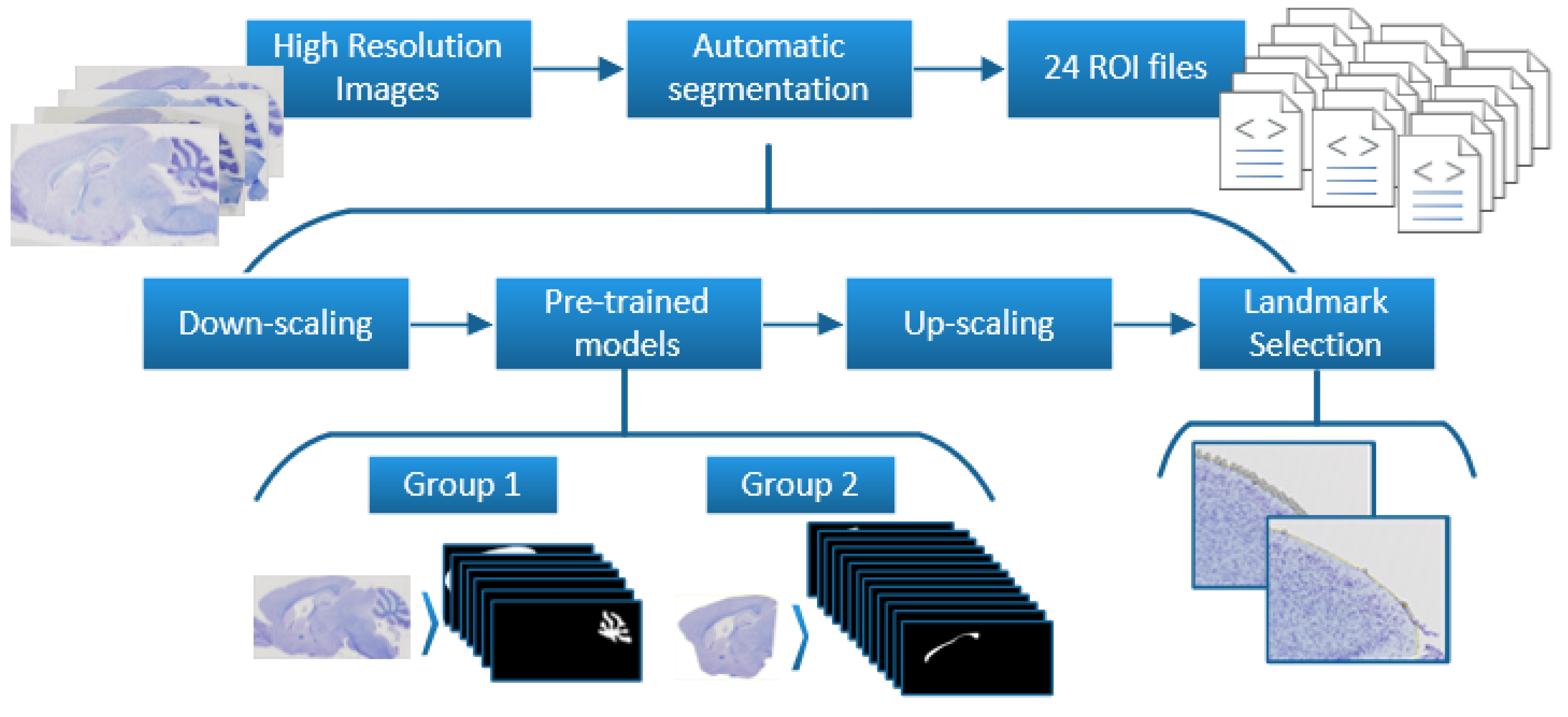
  • Image treatment (up/down-scaling, re-sampling, curve approximation) and conversion (ROI to PNG formats and vice versa) for initial and final steps of the training pipeline.
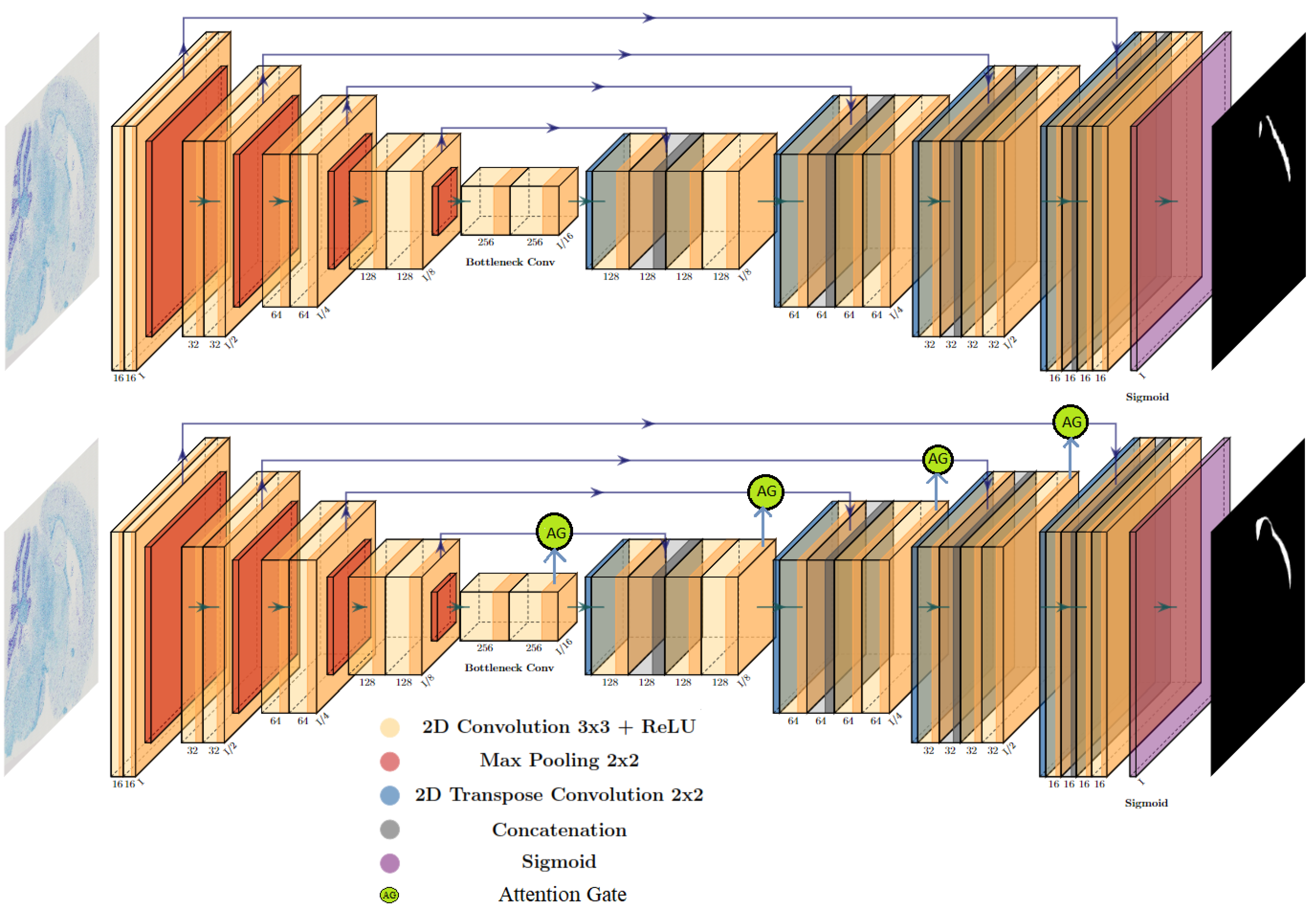
  • Training and test U-Net and Attention U-Net architectures with two different size of the images as input for the segmentation task.
  • Creation and deploy of a usable tool to automatically segment histological mouse brain images for 24 regions of interest, which would be significantly faster than human annotators.

2. Materials and Methods

The proposed automatic segmentation for the different regions of the mouse brain was divided into three main parts: dataset preparation, deep learning model, and image post-processing.

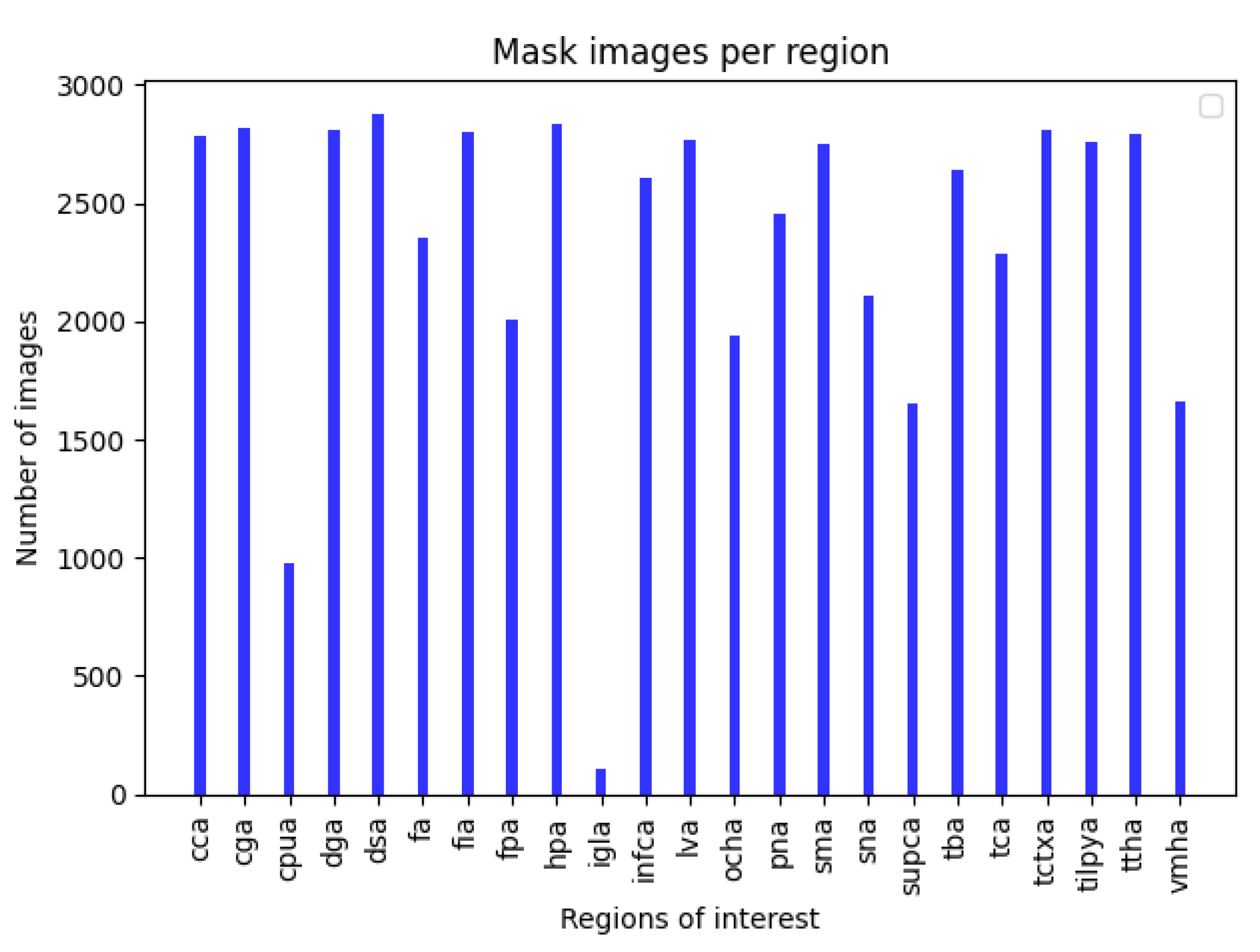
2.1. Dataset Preparation

The NeuroGEMM laboratory (INSERM Unit 1231, University of Burgundy, Dijon, France) currently hosts a database of 22,353 histological scanned 2D sections (parasagittal and coronal) of mouse brain samples manually curated and segmented. In our laboratory, over 75% of the brains included in the dataset were processed by two technicians (handling sectioning and staining). Additionally, 29 students, all trained by a single senior neuroanatomist, performed segmentation. This approach was designed to minimize inter-annotator variability in the training dataset.
In brief, brains from 14 to 16-week-old wild-type or mutant mice (knock-out or knock-in) were collected, fixed in paraformaldehyde, and embedded in paraffin. Sections of 5 μ m thickness were collected using a microtome, either in three coronal (Bregma +0.98, −1.34, −5.80 mm) or one parasagittal (Lat +0.6 mm) plane +/− 60 μ m. Sections were deparaffinized and stained with fast luxol blue revealing axons through labeling of myelin and cresyl violet which revealed cells via staining of Nissl bodies. High-resolution scanning of histological slides was performed using a dedicated scanner (NanoZoomer 2.0HT, Hamamatsu, Hamamatsu City, Japan) to obtain digitized slides with enough resolution to visualize individual cells. Quality control was conducted to assess critical section variation, symmetry, staining, and image quality. Brain anatomical parameters were measured using standard operating procedures using plug-ins developed in the ImageJ/Fiji software [16]. Measurements of surface areas and distances were manually annotated and saved in ROI format, which stores region-specific information. Figure 1 shows an example of visualization of the landmarks stored in the cerebellum annotation. Since the overarching goal of the data analysis is to identify morphogenes, all the analysis is performed genotype-blind until this step to avoid bias. Data were also checked for human error and outliers using a database and routines allowing automated outliers detection using the interquartile boundaries (1.2*IQR). Outliers due to plane asymmetries (asymmetrical sectioning relative to specific coordinates) or non-critical sectioning (plane selected before or after the critical plane) were removed. Extremes with no obvious reason were left as they may result from genetic mutations. A genotype “deblind” is then carried out to group brain samples based on genotype and identify novel morphogenes affecting brain structure [4]. Hence, the final dataset consists of images from normal and abnormal brains.
In this segmentation project, we worked with a parasagittal plane that is currently the main section used by the laboratory and the 24 regions of interest presented in Figure 2 and listed in Table 1.
The first step was the preparation of the dataset that was used to train several deep learning models. Due to the large size of the image files, a minimum workable resolution was evaluated as a trade-off between calculation time for training and annotation accuracy.

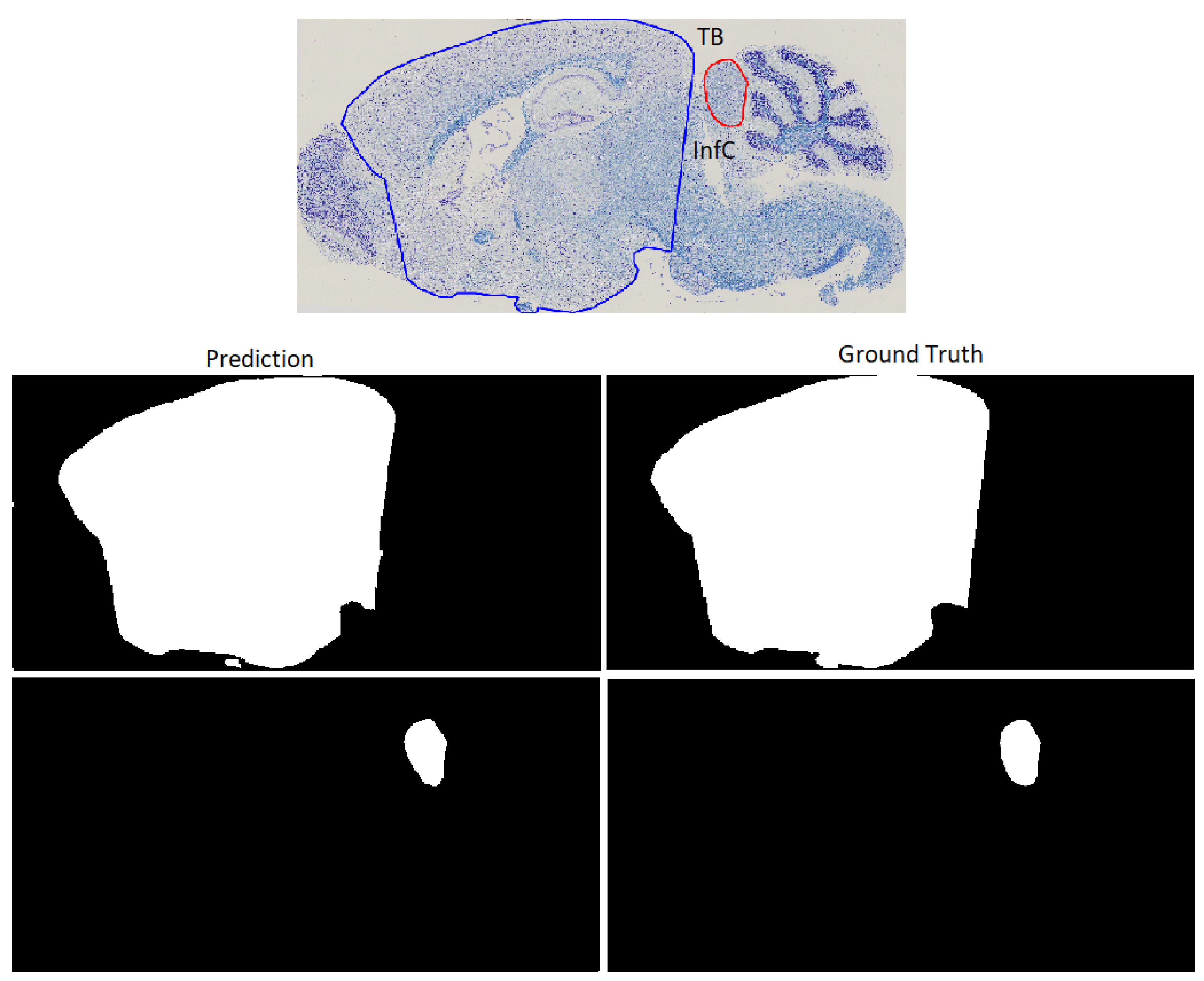
2.1.1. Landmarks to Binary Masks

The database was cross-checked for existence of both images and ROI files. With an initial amount of more than 2000 images in sagittal view, images and landmarks defined by the ROI file were then checked if they overlapped properly and matched in size. Regions were binarized, and their size reduced from high resolution (e.g., 24,000 pixels × 14,000 pixels) to 512 × 256 and 2048 × 1024 in order to fit scaled images using a bilinear interpolation algorithm at identical resolution.

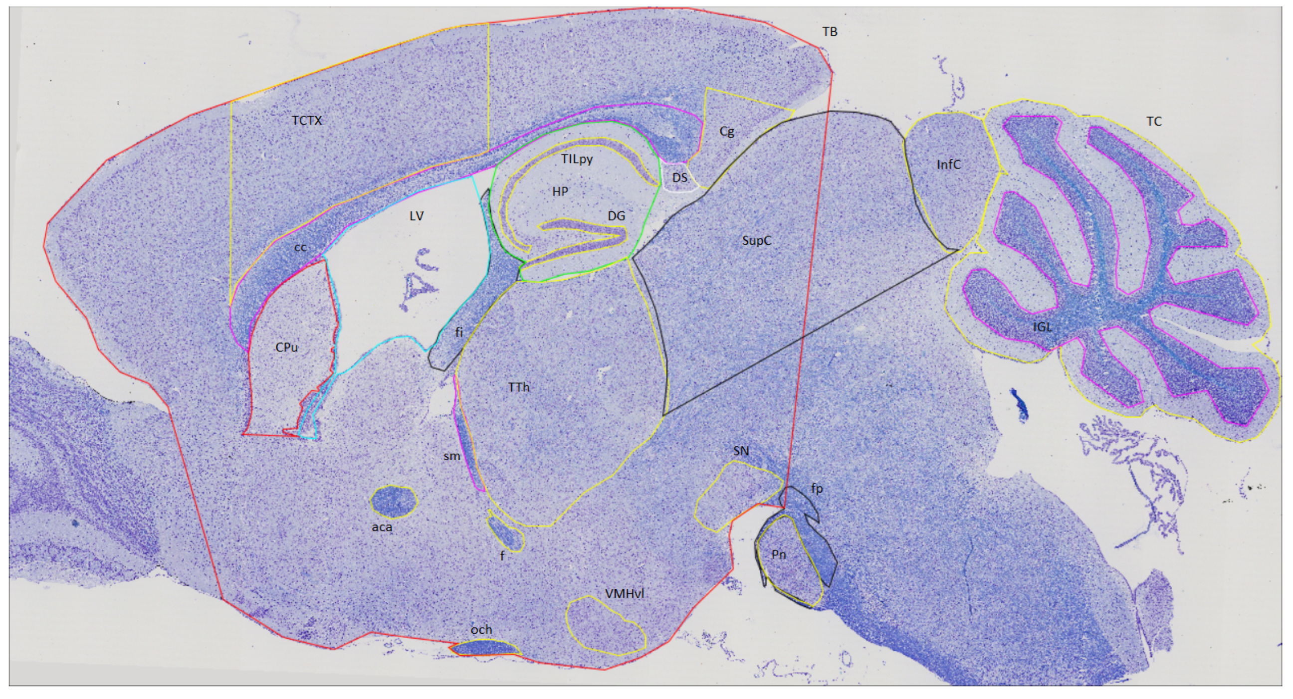
2.1.2. Brain Division

Brain regions of interest were then divided into two groups. The first group consisted of regions where the entire image were used as input to train the model. Meanwhile, for the second group, the total brain area (TB) was used as the working boundary area and only the regions within this area were localized. The division of all the neuroanatomical features is shown in Table 1.

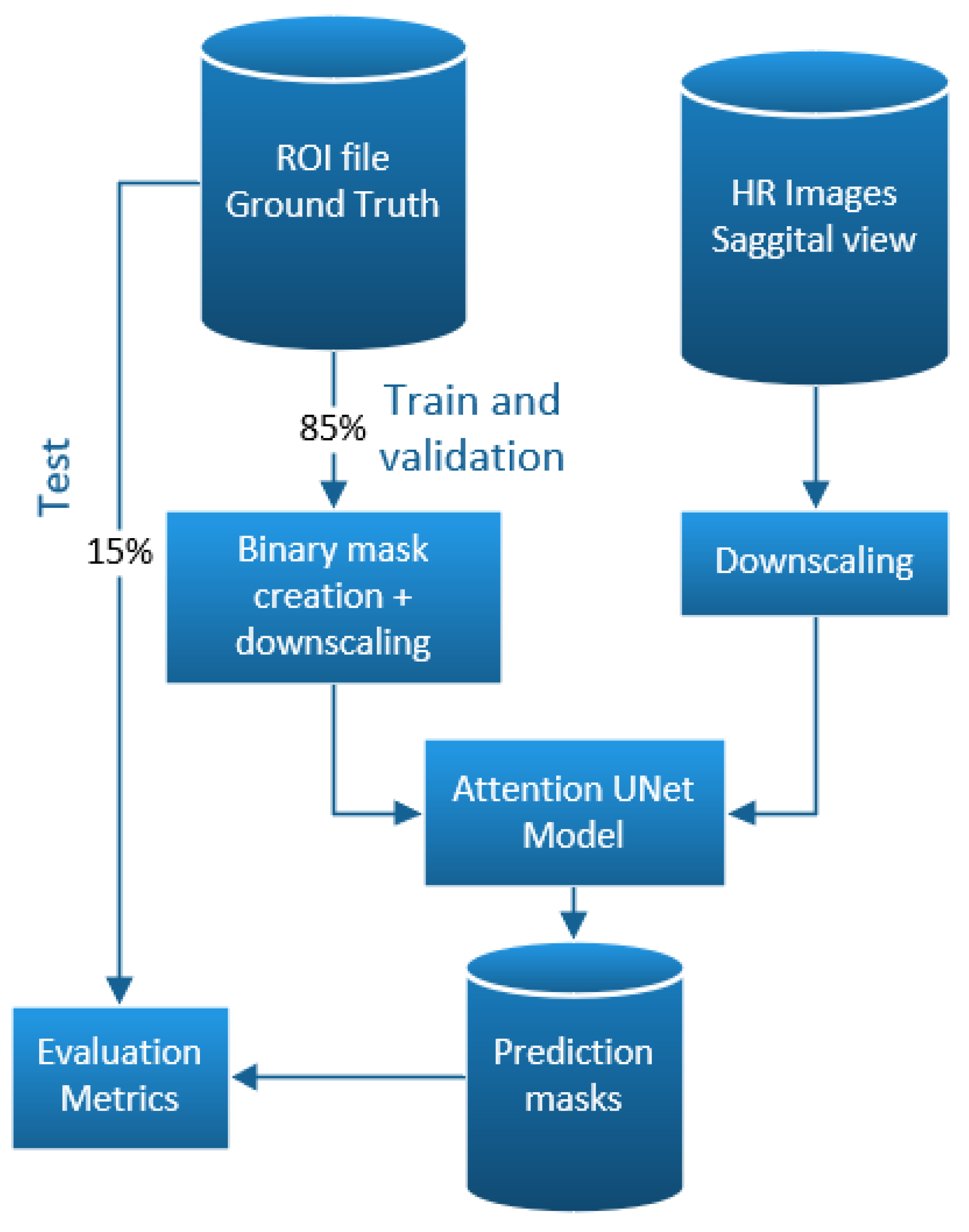
2.2. Deep Learning Models

Several deep learning models were tested. Initially, we chose to work and test these models at low resolution (512 × 256) to verify their ability to capture important features in the mouse brain.
The first tested model, U-Net, proposed by Ronneberger et al. [14], was used as a starting point to segment brain regions, since this architecture is considered as the method of reference in medical image segmentation. We chose to work with a depth of 5 levels and with feature maps in the encoder of 3, 16, 32, 64 and 128; and 256, 128, 64, 32 and 16 for the decoder, being the initial configuration of the architecture.
Each experiment was trained for 100 epochs with a minibatch size of 32 images. An Adam optimization was performed and weights were saved for the epoch that produced the last train iteration. A starting learning rate was fixed at 0.01 with a scheduler function that reduces the learning rate by a factor of 10 after 15 consecutive epochs. An early stopping function was implemented to make the model training process time efficient. The model was trained with the Pytorch framework using a NVIDIA A100 GPU.
Two different loss functions were tested, binary cross entropy with logits loss (BCE) and Dice loss. The Dice loss function was chosen because it offers better performance in the chosen evaluation metric (Dice Score Coefficient, DSC). Moreover, at the end of this round, using low definition images, it was concluded that the U-Net architecture was not able to acquire enough information to adequately delimit the regions of interest. Indeed, it was necessary to apply extensive post-processing of the images to improve segmentation. This model was thus discarded from the next round of testing which used low (521 × 256) and medium (2048 × 1024) resolutions.
The second tested model is based on the work of Hamida et al. [15], who proposed a weakly supervised method using Attention U-Net for colon cancer image segmentation. The addition of attention blocks dynamically weighs the importance of different image regions during the segmentation process. This enables the network to focus on relevant features and enhances the accuracy of the segmentation results. Initially, the same depth and features map as the previous architecture were maintained. Figure 3 presents a visual comparison between both architectures. Given the promising segmentation results, we decided to use an encoder/decoder feature maps consisting of 3, 64, 128, 256 and 512; and 1024, 512, 256, 128 and 64, respectively.
However, increasing the number of levels from 5 to 7 (encoder, 3, 64, 126, 256, 512, 1024, 2048 and decoder, 4096, 2048, 1024, 512, 256, 128, 64) gave better segmentation results while increasing the image resolution to 2048 × 1024.
In order to train and test the models, the database of all masks and images was divided into 3 groups. We used 70%, 15% and 15% for training, validation and testing, respectively. Once the training was finished, performances of the models were tested in the different regions and for the different resolutions previously established.

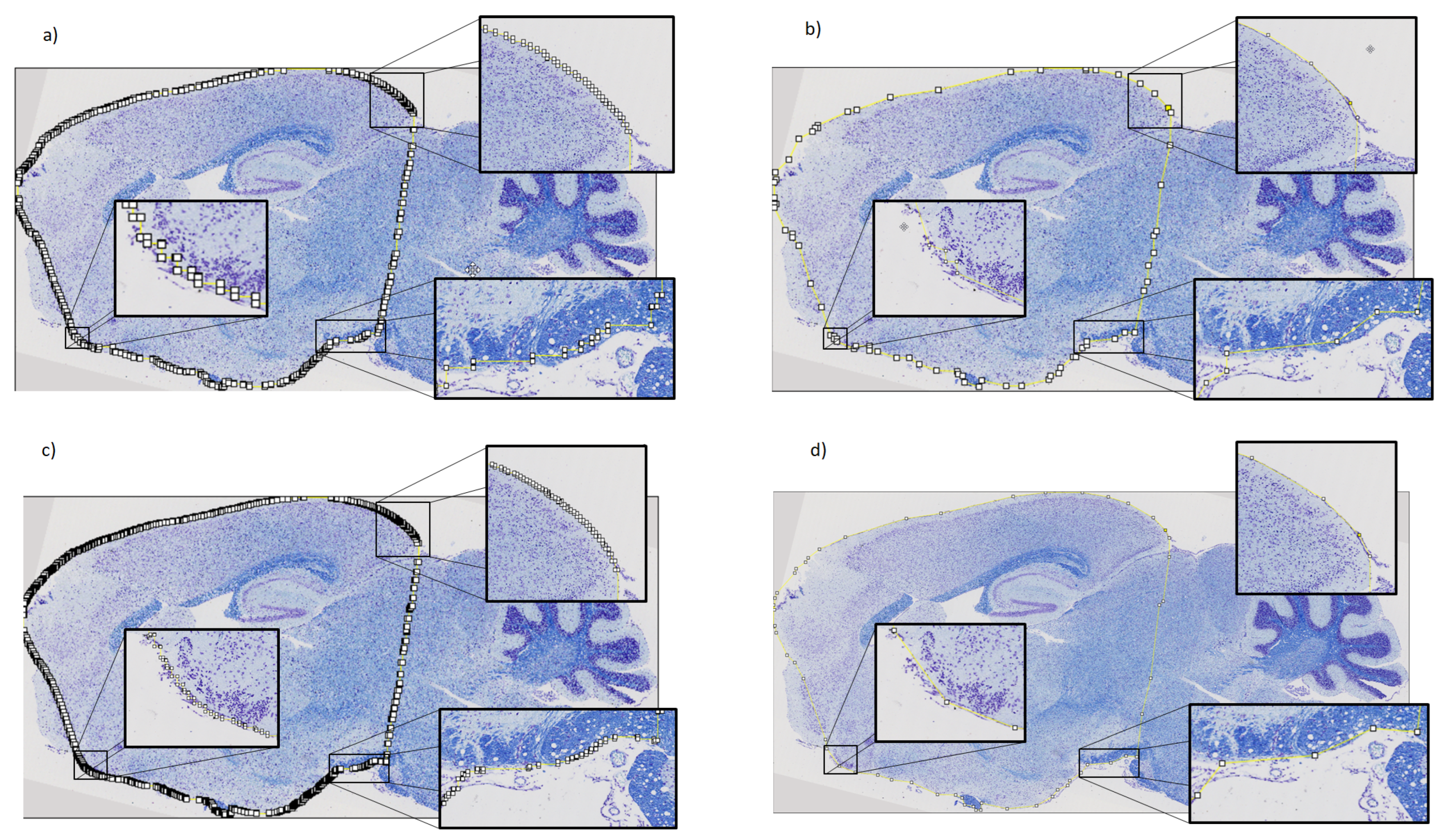
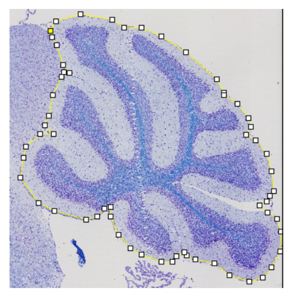
2.3. Refinement and Landmarks

After training the deep learning models for the two considered resolutions, resulting segmentations needed to be scaled back to the original size of the images. A bicubic interpolation algorithm was used but irregularities remained in the fine definition of the contour.
The Douglas–Peucker algorithm [17] was used to solve this problem. By iteratively calculating distances and selecting the point with the maximum distance from a line segment, the algorithm removes redundant points and simplifies the contour while retaining its essential characteristics. For example, Bimanjaya et al. used the same approach of refinement for the extraction of road network in urban area [18]. Several tests were performed to achieve a balance between the number of points delivered by the polygon contour from the binary mask, and the required accuracy in annotating the contour of the region of interest.
The final result consists of a set of landmarks grouped into a region of interest as an .ROI file usable by ImageJ for each of the 24 regions of interest. The number of landmarks can be different according to the size and the shape of the area.

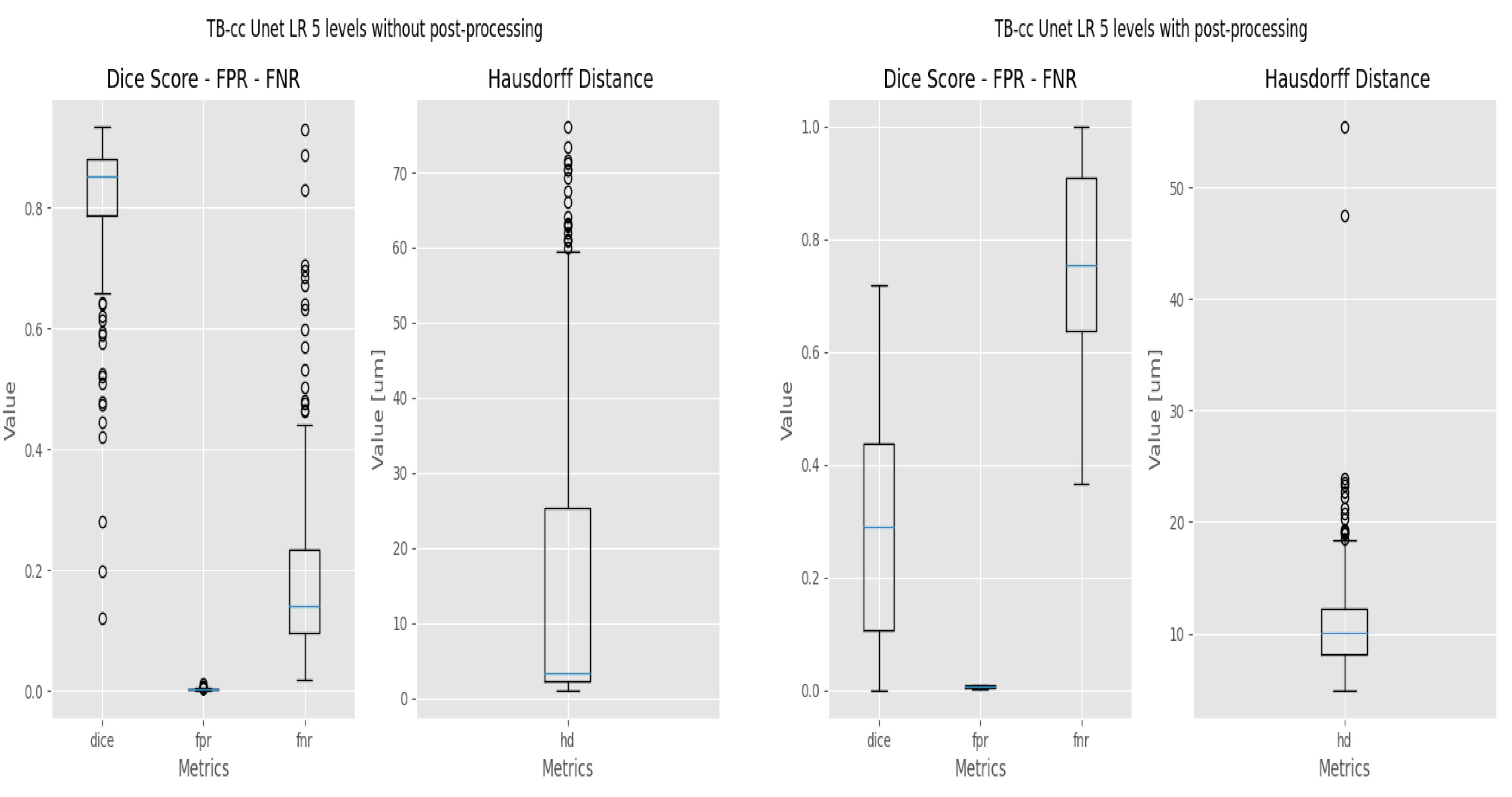
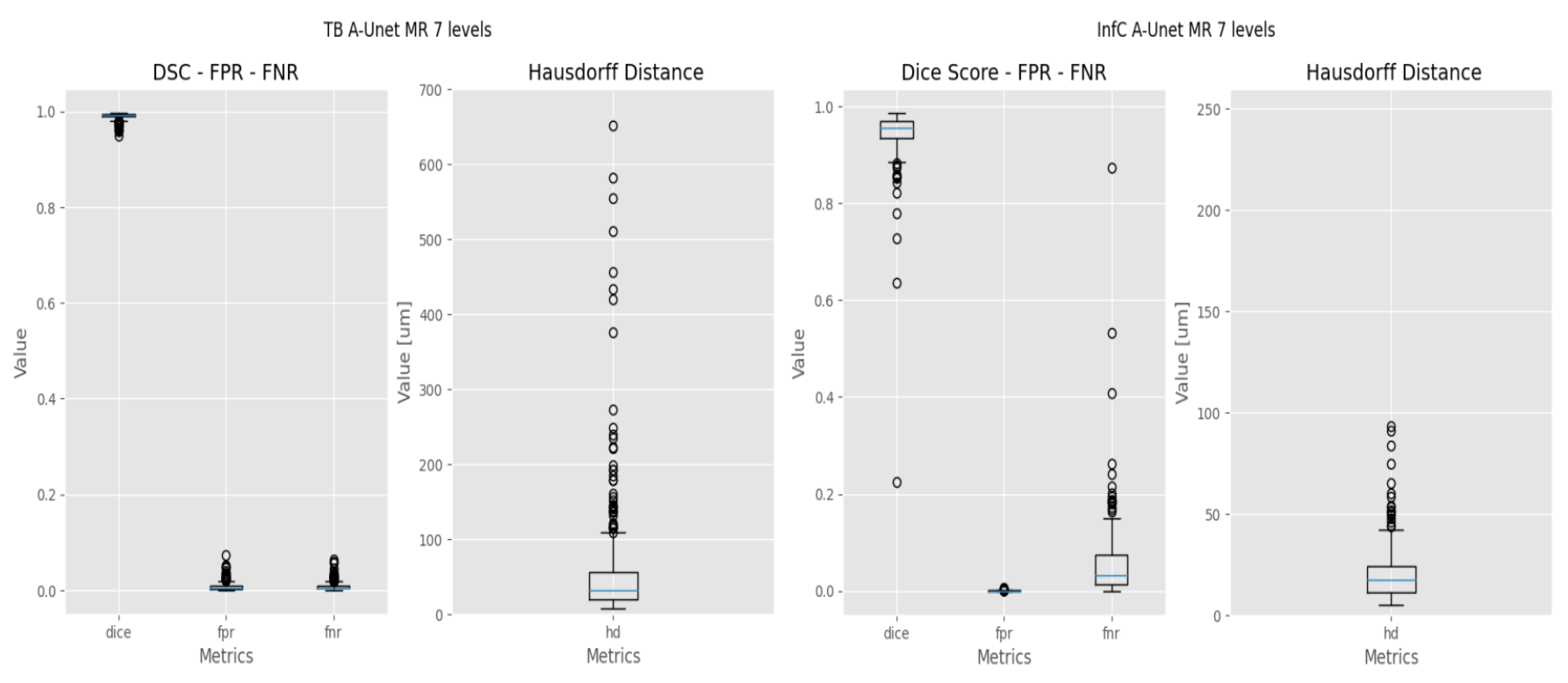
2.4. Evaluation Metrics

  • The Dice coefficient, or Dice similarity coefficient [19], is a metric commonly used to evaluate the accuracy of segmentation results (Equation (1)). It measures the overlap between the predicted segmentation and the ground truth by calculating the ratio of twice the intersection of the two regions to the sum of their sizes.
    Dice   coefficient = 2 I n t e r s e c t i o n P r e d i c t i o n + G r o u n d T r u t h
  • The False Positive Rate (FPR) [20] is a metric that measures the proportion of incorrect positive predictions made by the model (Equation (2)). A lower False Positive Rate indicates better performance, as it indicates a lower rate of false alarms or incorrect positive predictions.
    F P R = F P F P + T N
    where FP = False Positive, TN = True Negative.
  • The False Negative Rate (FNR). Ref. [20] measures the proportion of missed positive predictions by the model (Equation (3)). A lower False Negative Rate is desired as it signifies a lower rate of missed detections or incorrectly classified negatives, indicating better sensitivity and accuracy in capturing the target structure or region.
    F N R = F N F N + T P
    where TP = True Positive, FN = False Negative.
    Both FPR and FNR will be used to evaluate the response of the models at pixel level.
  • The Hausdorff Distance (HD) [21] measures the dissimilarity between two sets of points or contours (Equation (4)). It quantifies the maximum distance between any point in one set to the closest point in the other set.
    H D ( A , B ) = m a x ( m a x ( d ( a , B ) ) , m a x ( d ( b , A ) ) )
    where:
    • d(a, B) represents the minimum distance between a point a in set A and the closest point in set B.
    • d(b, A) represents the minimum distance between a point b in set B and the closest point in set A.

2.5. Implementation

The proposed method was integrated into existing analytical pipelines to allow neuroanatomists to continue annotating regions of interest in the mouse brain albeit more efficiently. Using a command line, the end user is now able to pre-analyze the images automatically and then run the existing analytical pipeline made of ImageJ macros to validate or edit the deep-learning generated regions of interest. For the end user, this results in faster (6 to 10X) image annotation times. Figure 4 shows the final pipeline of the model.
In Figure 5, an example of standard workflow for all the regions within the mouse brain is shown. As inputs we have, on the one hand, the masks of each of the regions of interest (up to 24 per brain), and on the other hand, about 2000 histological images of the mouse brain associated with these masks. Of the total number of target images, 85% are used for training and validation tasks. The remaining 15% were destined for testing. The regions of interest are converted to a format that can be used in the deep learning model (ROI format to PNG format) and then reduced in size to the size set for the study. In the same way, the size of the histological images is reduced. Afterwards, with both images reduced in size, we proceed to train the deep learning model (in this case, an Attention U-Net architecture). Once the model has been trained, the predicted masks are then stored and evaluated with the aforementioned evaluation metrics.
Once the network is correctly trained and with favorable responses for the segmentation of the regions of the mouse brain, we proceed to the implementation of the system that will be put into operation in the NeuroGeMM laboratory. Figure 4 shows the final pipeline implemented to segment 24 region of interest within the mouse brain. This system accepts high-definition histological images as input and delivers up to 24 regions of interest found in the input image as output. This process is performed by the automatic segmentation of the regions thanks to the previous trained network. The main constituent parts to fulfill this purpose are: size reduction, region prediction, size increase, and finally the selection of points of interest for storage in ROI format.

3. Results

3.1. Data Preparation

Database checks identified a small number of mislabeled regions of interest but the vast majority of missing ROIs were down to asymmetries, histological artifacts or non critical sectioning. Figure 6 shows the number of mask images per area of interest. Based on the binary masks created for all the regions, it was found that several regions overlapped due to the sub-accuracy of the manual segmentation. Thus, it was proposed to create individual segmentation models for each the region of interest instead of a multi-class approach.

3.2. Deep Learning

Training results with the U-Net architecture are presented for three different regions of the mouse brain in Figure 7. The input images have a size of 512 pixels by 256 pixels.
Morphological operations such as dilation and erosion were applied to fill in incomplete areas and in some cases to eliminate erroneously segmented pixels. Figure 8 presents the results of post-processing for corpus callosum segmentation with the same U-Net architecture.
The evaluation metrics obtained following these morphological operations decrease and needed to be tailored to each image. And anyways, the poor performance of the U-Net is evident. The switch to an Attention U-Net, where gates focus the training on the regions of interest [15]m yielded better results even with low resolution images (512 × 256 pixels) and an architecture depth of five levels. With a higher input resolution images of 2048 × 1024 pixel and an architecture depth of seven levels, the best results were obtained (see Figure 9), even without post-processing.
In Figure 10, the output evaluations metrics for the training with Attention U-Net for TB and InfC is shown.
Results for the Attention U-Net with seven levels and 2048 × 1024 image resolution are presented in Table 2. Highest DSC (Equation (1)) were obtained for the TB (total brain) with 99.14% whilst worst performance was obtained for the fp (fibers of the pons) with (70.47%). This model reaches an overall DSC of 0.90 ± 0.01.

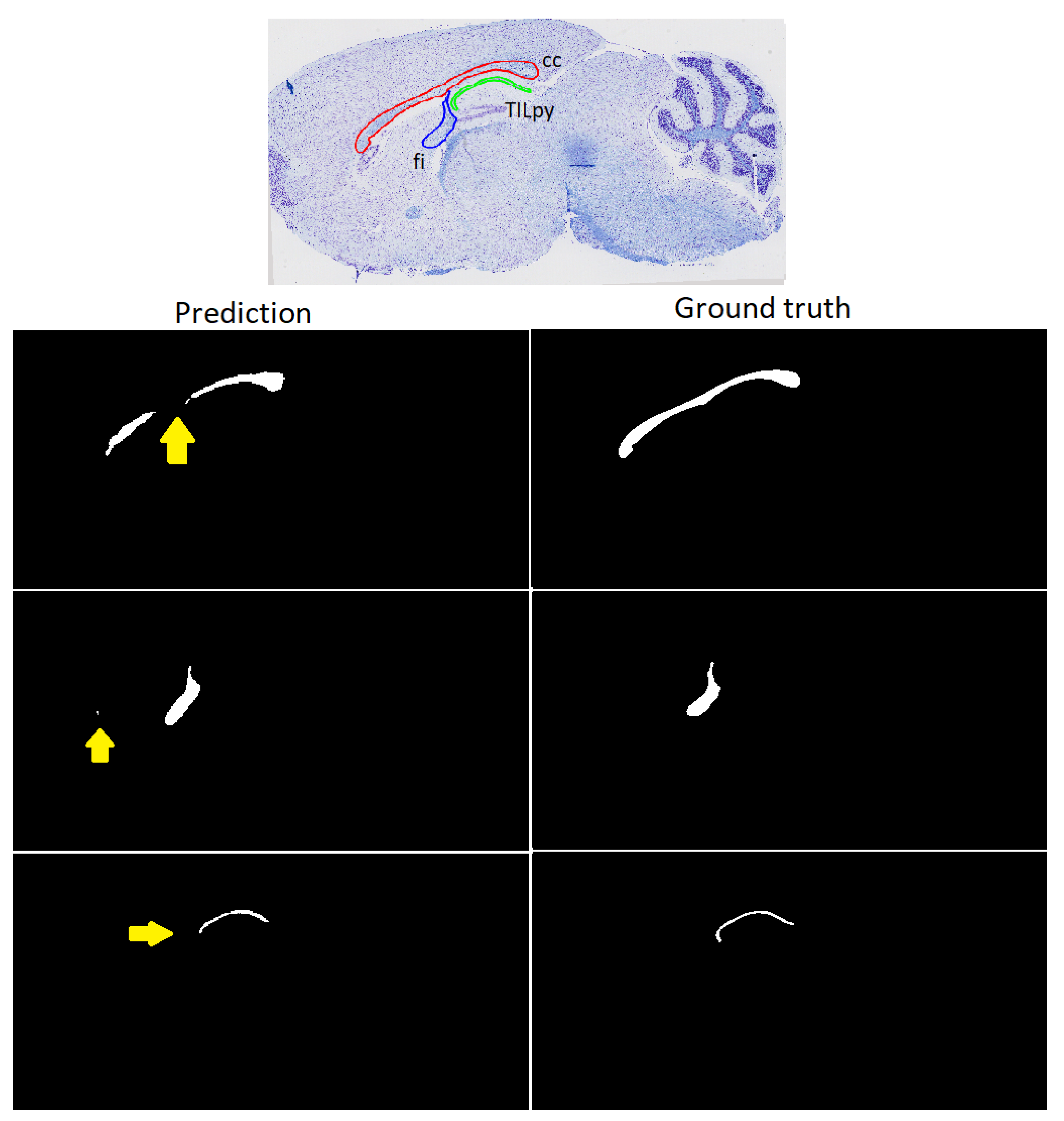
3.3. Refinement and Landmark

As a last step, the masks are converted from binary images to point vectors so that they can be visualized/edited using the Fiji/ImageJ software. Figure 11 compares the post-processing performance with the two different resolutions (512 × 256 and 2048 × 1028). For the TBA, working with 2048 × 1028 images resulted in landmarks at near equal distance from each other than what would have been chosen by a human user making edits possible. In the end, the time to compile an image takes approximately 5 min, although this task is completely automated and was scripted to process folders containing many images.

4. Discussion

In this article, we introduce a versatile approach for the automatic segmentation of mouse brain histological samples, addressing the time-intensive challenge of manual annotation. This is particularly valuable for high-throughput projects, where implementing efficient segmentation strategies is crucial.
Our work presents advances in the resolution time of the segmentation task, reducing the segmentation period to 5–7 min per image in comparison with Yates et al. [8], which performs 60 images in less than 24 h. Similarly, in the accuracy in segmenting rodent brain regions, Xu et al. provided a DSC close to 90% on average as for the hippocampus [11], while our proposal reaches 98% DSC on average.
Our proposed approach establishes a robust foundation for generating accurate mouse brain landmarks, emphasizing the strategic choice of models. We prioritized achieving high-quality, human-comparable segmentation with simpler, well-established architectures like U-Net and its attention-augmented variant over more complex models such as EfficientNet. This decision aligns with making advanced segmentation techniques more accessible to the broader research community.
In their respective projects, Mesejo et al. [12] and Barzekar et al. [13] developed tools to segment a maximum of two regions of interest, separated by a decade of technological advancements. Remarkably, Mesejo et al.’s system was introduced 11 years ago, a time when computational resources were limited. Comparatively, their model achieved a 92.25% accuracy in hippocampus segmentation, while our approach reached a DSC of 98.48%. Similarly, Barzekar et al. reported DSCs of 86.78% and 79.28% for specific brain regions, while our model achieved 76.47% for the substantia nigra. These comparisons indicate modest improvements in accuracy and highlight that some brain regions are more easily segmented than others, and that more advanced models do not always yield higher DSCs.
Our comparison of U-Net and Attention U-Net architectures reveals that the incorporation of attention gates significantly improves segmentation tasks. For example, segmentation of the corpus callosum with U-Net achieved a DSC of 80%, which improved to approximately 94% with Attention U-Net. This underscores the importance of attention mechanisms, particularly for intricate brain structures. The efficacy of attention gates is further demonstrated by our model’s consistent focus on the right regions, evidenced by low false positive ratio values, and achieving a 99.14% DSC for the total brain area.
However, regions like the caudate putamen and fibers of the pons posed greater challenges due to factors such as cellular-level grouping, genetic variation, and inconsistencies across specimens. Despite these difficulties, our model attained DSCs of 79.18% and 70.47% for these regions. Notably, deep-learning segmentation of the VMH was successful despite the belief that cell shapes are critical for manual segmentation. This suggests that ultra-high-resolution imaging, typically a significant challenge for deep learning, is not always essential for accurate segmentation.
Our model’s modular design allows each part to be substituted or improved, enhancing its versatility. We have implemented this model in our laboratory to annotate up to 24 brain regions, streamlining user interaction through a single command line. The training dataset was sourced from studies examining data structure drifts [4]. The model is also suitable for interobserver studies to assess variability among regions and anatomists. One of the limitations of our work is that the study was performed only on sagittal view images; work is currently being performed on the coronal view. On the other hand, the variability that exists among the different annotators made it difficult to correctly automatically recognize regions of interest such as the caudate putamen. Future work to be performed is how to take the inter-annotatator variability into account.
Our study demonstrates that strategic model choices and augmentations like attention mechanisms facilitate high-quality segmentation on histological images without relying on the most complex deep learning architectures. Moreover, these tools are becoming increasingly accessible to most laboratories. Paradoxically, while new technological advances are flourishing in 3D histology [22], they bring challenges in data analysis akin to those in other modalities like MRI and microCT. Our laboratory is now embracing these advancements by processing brains in 3D using block face serial imaging. While the voxel resolution in this method is ten times higher than what current MRI technologies offer for rodent brains [23], it is clear that much of the groundwork in automated segmentation will likely stem from these studies since they have long established that manually segmenting 3D volumes poses even greater challenges.

5. Conclusions

In this work, we proposed an automatic solution to automatically segment 24 regions of interest sagittal histological images of mouse brains. The proposed model produces excellent results for all of the areas, and provides a starting point for the investigation of more accurate histological image segmentation systems. The model, apart from being easy to manage, does not require any additional software or training of the laboratory staff to use it. The system accepts as input a given type of histological images and automatically converts them into landmarks of the regions of interest of the mouse brain. It takes as little as 5 min to correctly determine 24 regions, mainly due to validation and correction if necessary, as opposed to an average of 1 h to perform the same task manually. The final results are ROI files of the analyzed regions, which can be used by classical medical image software to perform the different neuroanatomical studies.

Author Contributions

Conceptualization, A.L., F.M. and S.C.; methodology, J.C., A.L., F.M. and S.C.; software, J.C., A.L. and F.M.; validation, J.C., A.L., F.M. and S.C.; formal analysis, A.L., F.M. and S.C.; investigation, J.C., A.L., F.M. and S.C.; resources, A.L., S.C. and B.Y.; data curation, S.C. and B.Y.; writing—original draft preparation, J.C., A.L., F.M. and S.C.; writing—review and editing, A.L., F.M. and S.C.; supervision, A.L., F.M. and S.C. All authors have read and agree to the published version of the manuscript.

Funding

This research received no external funding.

Data Availability Statement

Belonging to the NeuroGeMM laboratory (Dijon, France), data cannot be shared publicly without the permission of this center. However, they are available upon request.

Conflicts of Interest

The authors declare no conflict of interest.

References

  1. Bossert, L.; Hagendorff, T. Animals and AI. The role of animals in AI research and application—An overview and ethical evaluation. Technol. Soc. 2021, 67, 101678. [Google Scholar] [CrossRef]
  2. Collins, F.S.; Rossant, J.; Wurst, W. A mouse for all reasons. Cell 2007, 128, 9–13. [Google Scholar] [PubMed]
  3. Mohun, T.; Adams, D.J.; Baldock, R.; Bhattacharya, S.; Copp, A.J.; Hemberger, M.; Houart, C.; Hurles, M.E.; Robertson, E.; Smith, J.C.; et al. Deciphering the Mechanisms of Developmental Disorders (DMDD): A new programme for phenotyping embryonic lethal mice. Dis. Model. Mech. 2013, 6, 562–566. [Google Scholar] [CrossRef] [PubMed]
  4. Collins, S.; Mikhaleva, A.; Vrcelj, K.; Vancollie, V.; Wagner, C.; Demeure, N.; Whitley, H.; Kannan, M.; Balz, R.; Anthony, L.; et al. Large-scale neuroanatomical study uncovers 198 gene associations in mouse brain morphogenesis. Nat. Commun. 2019, 10, 3465. [Google Scholar] [CrossRef] [PubMed]
  5. Kretz, P.F.; Wagner, C.; Montillot, C.; Hugel, S.; Morella, I.; Kannan, M.; Mikhaleva, A.; Fischer, M.C.; Milhau, M.; Brambilla, R.; et al. Dissecting the autism-associated 16p11. 2 locus identifies multiple drivers in brain phenotypes and unveils a new role for the major vault protein. Genome Biol. 2023, in press. [Google Scholar]
  6. Groeneboom, N.E.; Yates, S.C.; Puchades, M.A.; Bjaalie, J.G. Nutil: A pre-and post-processing toolbox for histological rodent brain section images. Front. Neuroinform. 2020, 14, 37. [Google Scholar] [CrossRef] [PubMed]
  7. Xu, H.; Liu, L.; Lei, X.; Mandal, M.; Lu, C. An unsupervised method for histological image segmentation based on tissue cluster level graph cut. Comput. Med. Imaging Graph. 2021, 93, 101974. [Google Scholar] [CrossRef] [PubMed]
  8. Yates, S.C.; Groeneboom, N.E.; Coello, C.; Lichtenthaler, S.F.; Kuhn, P.H.; Demuth, H.U.; Hartlage-Rübsamen, M.; Roßner, S.; Leergaard, T.; Kreshuk, A.; et al. QUINT: Workflow for quantification and spatial analysis of features in histological images from rodent brain. Front. Neuroinform. 2019, 13, 75. [Google Scholar] [CrossRef] [PubMed]
  9. Puchades, M.A.; Csucs, G.; Ledergerber, D.; Leergaard, T.B.; Bjaalie, J.G. Spatial registration of serial microscopic brain images to three-dimensional reference atlases with the QuickNII tool. PLoS ONE 2019, 14, e0216796. [Google Scholar] [CrossRef] [PubMed]
  10. Sommer, C.; Straehle, C.; Koethe, U.; Hamprecht, F.A. Ilastik: Interactive learning and segmentation toolkit. In Proceedings of the 2011 IEEE International Symposium on Biomedical Imaging: From Nano to Macro, Chicago, IL, USA, 30 March–2 April 2011; pp. 230–233. [Google Scholar]
  11. Xu, X.; Guan, Y.; Gong, H.; Feng, Z.; Shi, W.; Li, A.; Ren, M.; Yuan, J.; Luo, Q. Automated brain region segmentation for single cell resolution histological images based on Markov random field. Neuroinformatics 2020, 18, 181–197. [Google Scholar] [CrossRef] [PubMed]
  12. Mesejo, P.; Ugolotti, R.; Cagnoni, S.; Di Cunto, F.; Giacobini, M. Automatic segmentation of hippocampus in histological images of mouse brains using deformable models and random forest. In Proceedings of the 2012 25th IEEE International Symposium on Computer-Based Medical Systems (CBMS), Rome, Italy, 20–22 June 2012; pp. 1–4. [Google Scholar]
  13. Barzekar, H.; Ngu, H.; Lin, H.H.; Hejrati, M.; Valdespino, S.R.; Chu, S.; Bingol, B.; Hashemifar, S.; Ghosh, S. Multiclass Semantic Segmentation to Identify Anatomical Sub-Regions of Brain and Measure Neuronal Health in Parkinson’s Disease. arXiv 2023, arXiv:2301.02925. [Google Scholar]
  14. Ronneberger, O.; Fischer, P.; Brox, T. U-Net: Convolutional Networks for Biomedical Image Segmentation. In Proceedings of the Medical Image Computing and Computer-Assisted Intervention–MICCAI 2015: 18th International Conference, Munich, Germany, 5–9 October 2015; Proceedings, Part III. pp. 234–241. [Google Scholar]
  15. Hamida, A.B.; Devanne, M.; Weber, J.; Truntzer, C.; Derangère, V.; Ghiringhelli, F.; Forestier, G.; Wemmert, C. Weakly Supervised Learning using Attention gates for colon cancer histopathological image segmentation. Artif. Intell. Med. 2022, 133, 102407. [Google Scholar] [CrossRef] [PubMed]
  16. Collins, S.C.; Wagner, C.; Gagliardi, L.; Kretz, P.F.; Fischer, M.C.; Kessler, P.; Kannan, M.; Yalcin, B. A method for parasagittal sectioning for neuroanatomical quantification of brain structures in the adult mouse. Curr. Protoc. Mouse Biol. 2018, 8, e48. [Google Scholar] [CrossRef] [PubMed]
  17. Visvalingam, M.; Whyatt, J.D. The Douglas-Peucker algorithm for line simplification: Re-evaluation through visualization. In Computer Graphics Forum; Wiley Online Library: Hoboken, NJ, USA, 1990; Volume 9, pp. 213–225. [Google Scholar]
  18. Bimanjaya, A.; Handayani, H.H.; Rachmadi, R.F. Extraction of Road Network in Urban Area from Orthophoto Using Deep Learning and Douglas-Peucker Post-Processing Algorithm. In IOP Conference Series: Earth and Environmental Science; IOP Publishing: Bristol, UK, 2023; Volume 1127, p. 012047. [Google Scholar]
  19. Zou, K.H.; Warfield, S.K.; Bharatha, A.; Tempany, C.M.; Kaus, M.R.; Haker, S.J.; Wells, W.M., III; Jolesz, F.A.; Kikinis, R. Statistical validation of image segmentation quality based on a spatial overlap index1: Scientific reports. Acad. Radiol. 2004, 11, 178–189. [Google Scholar] [CrossRef] [PubMed]
  20. Fernandez-Moral, E.; Martins, R.; Wolf, D.; Rives, P. A new metric for evaluating semantic segmentation: Leveraging global and contour accuracy. In Proceedings of the 2018 IEEE Intelligent Vehicles Symposium (iv), Changshu, China, 26–30 June 2018; pp. 1051–1056. [Google Scholar]
  21. Sudha, N. Robust Hausdorff distance measure for face recognition. Pattern Recognit. 2007, 40, 431–442. [Google Scholar]
  22. Walsh, C.; Holroyd, N.A.; Finnerty, E.; Ryan, S.G.; Sweeney, P.W.; Shipley, R.J.; Walker-Samuel, S. Multifluorescence high-resolution episcopic microscopy for 3D imaging of adult murine organs. Adv. Photonics Res. 2021, 2, 2100110. [Google Scholar] [CrossRef]
  23. Scharrenberg, R.; Richter, M.; Johanns, O.; Meka, D.P.; Rücker, T.; Murtaza, N.; Lindenmaier, Z.; Ellegood, J.; Naumann, A.; Zhao, B.; et al. TAOK2 rescues autism-linked developmental deficits in a 16p11. 2 microdeletion mouse model. Mol. Psychiatry 2022, 27, 4707–4721. [Google Scholar] [CrossRef] [PubMed]
Figure 1. Landmarks, manually taken, for the Cerebellum (TC).
Algorithms 16 00553 g001
Figure 2. Regions of interest taken by human user within the mouse brain in parasagittal view at Lateral +0.60 mm.
Algorithms 16 00553 g002
Figure 3. Comparison between U-Net (top) vs. Attention U-Net (bottom) architectures for training corpus callosum segmentation as an example. Inputs are high-resolution images and outputs are 24 regions of interest (ROIs) generated by the deep learning model.
Algorithms 16 00553 g003
Figure 4. Overall pipeline of the proposed method. Top: Input (high-resolution images) and Output (24 regions of interest, ROIs) used or generated by the deep learning model. The process of automated segmentation is delineated into several steps: downscaling of images, pretraining based on the specific group to which each ROI belongs, upscaling of the mask, and conversion of the mask to landmarks.
Algorithms 16 00553 g004
Figure 5. Workflow proposed to evaluate the accuracy of the training of a specific network. This example is for Attention U-Net in medium resolution 2048 × 1024.
Algorithms 16 00553 g005
Figure 6. Number of mask images per area of interest.
Algorithms 16 00553 g006
Figure 7. Left to right: prediction of the regions from U-Net architecture and ground truth masks for (top) corpus callosum, (middle) fimbria, (bottom) pyramidal cell layer TILpy. Yellow arrows show the areas where there is the greatest difference with respect to ground truth.
Algorithms 16 00553 g007
Figure 8. Results before and after applying morphological operations (as post-processing) for the segmentation of the corpus callosum using U-Net.
Algorithms 16 00553 g008
Figure 9. Left to right: predictions for (top) total brain area TB and (bottom) inferior colliculus InfC with a 7 levels Attention U-Net.
Algorithms 16 00553 g009
Figure 10. Results for TB (left) and InfC (right) while training with the images with resolution of 2048 × 1028 and with a 7-level Attention U-Net.
Algorithms 16 00553 g010
Figure 11. Example of converting contours to landmarks for the total brain area. (a) Original number of points (805) in 512 × 256 resolution. (b) Output landmarks (76) with resolution images in (a). (c) Original number of points (1501) with 2048 × 1024 resolution images. (d) Final landmarks (56) with resolution images in (c).
Algorithms 16 00553 g011
Table 1. Neuroanatomical features. To train the deep learning model for images in group 1, the entire image was used as input. Meanwhile, for images in group 2, the total brain region was used as input.
GROUP 1GROUP 2
NameTagNameTagNameTag
Inferior ColliculusInfCanterior commisureacaHippocampusHP
Superior ColliculusSupCcorpus callosumccLateral VentricleLV
Intra Granular LayerIGLCingulate cortexCgoptic chiasmoch
Total CerebellumTCCaudate PutamenCPustria medularissm
Substancia NigraSNDentate GyrusDGTotal Cortical areaTCTX
Pontine nucleusPnDorsal SubiculumDSpyramidal cell layerTILpy
fibers of the ponsfpfornixfThalamusTTH
Total BrainTBfimbriafiVentro Median HypothalamusVMHvl
Table 2. Results after image post-processing with an Attention U-Net with 7 levels and 2048 × 1024 resolution images. Evaluation metrics: DSC, Dice score coefficient; FPN, False Positive rate; FNR, False Negative rate; HD, Hausdorff distance; all of them with their standard deviation (STD). The best values are highlighted in bold and the worst values are emphasized in bold italics.
TAGDSCFPRFNRHD μ m
aca0.9660 ± 0.03940.0001 ± 0.00010.0276 ± 0.0573 5.2889 ± 11.0271
cc0.9365 ± 0.03470.0012 ± 0.00070.0421 ± 0.046315.1756 ± 14.8965
f0.8828 ± 0.09570.0001 ± 0.00020.0822 ± 0.116112.686 ± 40.1613
fi0.9179 ± 0.0810.0004 ± 0.00040.0798 ± 0.103527.9981 ± 28.0597
fp0.7047 ± 0.17580.0013 ± 0.00150.2383 ± 0.218466.8368 ± 52.7969
och0.9214 ± 0.08010.0001 ± 0.00020.0613 ± 0.102112.8222 ± 22.2288
sm0.8775 ± 0.09270.0003 ± 0.00040.0997 ± 0.125631.4965 ± 52.4748
TB0.9914 ± 0.00620.0079 ± 0.00850.0078 ± 0.00842.9213 ± 42.1242
TCTX0.978 ± 0.0280.0010 ± 0.00080.0205 ± 0.038720.3151 ± 28.2891
TC0.9902 ± 0.00530.001 ± 0.00060.0087 ± 0.008324.1482 ± 23.9261
IGL0.9267 ± 0.08650.0036 ± 0.00420.0546 ± 0.12433.7096 ± 43.5162
LV0.9452 ± 0.10690.0005 ± 0.0010.0493 ± 0.105841.9781 ± 64.002
TTh0.9515 ± 0.02680.0021 ± 0.00170.0492 ± 0.043534.1868 ± 16.472
CPu0.7918 ± 0.26140.001 ± 0.00130.1846 ± 0.265443.735 ± 42.5232
HP0.9848 ± 0.00680.0004 ± 0.00020.0122 ± 0.010912.6344 ± 7.6397
TILpy0.8852 ± 0.08120.0003 ± 0.00010.0814 ± 0.10518.8284 ± 24.7633
DG0.9302 ± 0.0770.0002 ± 0.00020.0465 ± 0.08628.0014 ± 11.5809
Pn0.9500 ± 0.0600.0002 ± 0.00020.0391 ± 0.06679.2620 ± 8.7277
SN0.7647 ± 0.19580.0006 ± 0.00070.2014 ± 0.218428.2791 ± 20.1335
Cg0.9087 ± 0.06120.0007 ± 0.00060.0817 ± 0.087323.341 ± 19.6141
DS0.8842 ± 0.07840.0001 ± 0.00010.1012 ± 0.110310.8247 ± 6.6032
InfC0.9442 ± 0.06130.0006 ± 0.00050.0542 ± 0.078419.608 ± 13.8624
SupC0.9483 ± 0.02490.0035 ± 0.00320.0479 ± 0.036411.7670 ± 6.0383
VMHvl0.8039 ± 0.17540.0005 ± 0.00040.1797 ± 0.209523.7869 ± 23.7924
Disclaimer/Publisher’s Note: The statements, opinions and data contained in all publications are solely those of the individual author(s) and contributor(s) and not of MDPI and/or the editor(s). MDPI and/or the editor(s) disclaim responsibility for any injury to people or property resulting from any ideas, methods, instructions or products referred to in the content.

