Dynamic Demand-Responsive Feeder Bus Network Design for a Short Headway Trunk Line

Abstract

Recent advancements in technology have increased the potential for demand-responsive feeder transit services to enhance mobility in areas with limited public transit access. For long rail headways, feeder bus network algorithms are straightforward, as the maximum feeder service cycle time is determined by rail headway, and bus–train matching is unnecessary. However, for short rail headways, the algorithm must address both passenger–feeder-bus and feeder-bus–train matching. This study presents a simulated annealing (SA) algorithm for flexible feeder bus routing, accommodating short headway trunk lines and multiple bus relocations for various stations and trains. A 5 min headway rail trunk line example was utilized to test the algorithm. The algorithm effectively managed bus relocations when optimal routes were infeasible at specific stations. Additionally, the algorithm minimized total costs, accounting for vehicle operating expenses and passenger in-vehicle travel time costs, while considering multiple vehicle relocations.

1. Introduction

The modal share for ridesharing has been in decline over the past few decades; however, it still has played an important role in mobility as one of the influencing travel modes in the United States [1]. There has been significant consideration given to on-demand ride services in recent years from federal and state governments and private sectors for improving on-demand transit services, especially in areas with limited accessibility to public transit services. Fewer mobility options are available in suburban areas because of weaker production/attraction centers of trips in a relatively large area and unpredictable travel demand based on low population density [2]. The flexible demand-responsive transit system (DRT), as an on-demand ride service, has been considered as an efficient mobility option in urban and suburban areas in many studies; however, the efficiency of these systems is open to discussion because of the different approaches and perspectives toward considering passengers and operator costs [3,4]. Generally, DRT systems have been proved in past studies as transit systems capable of satisfying even large transit demands and as a complementary transit mode that supports conventional transit systems [5]. Considering the advancement of new communication and computational technologies in transportation and transit systems such as automation and connectivity of vehicles, the demand-responsive transit systems with time windows (DRTTW) can take advantage of these technologies to improve the quality of service and maximize serving demands.

The proposed DRT feeder system in the current study performs as a complementary transit system with a rail system. A feeder system should follow routes and timetables to match demand requests to maximize demand coverage while improving the quality of service by maximizing fleet efficiency [6]. However, the perspectives of passengers and operators using a DRT system are different. From users’ perspective, their in-vehicle travel time should be minimized; therefore, direct routes are preferable for them because this will decrease their travel time and consequently the total passengers’ travel cost. On the other hand, the operator seeks to minimize vehicles’ traveled distances because that will decrease vehicle travel time and consequently the total transit operational costs. This problem should consider both user and operator costs at the same time as total costs, and therefore, it has a complex structure. In past studies, it has been introduced as an NP-Hard problem that should be solved by heuristics and metaheuristic methods [7].

Previously, an algorithm for a feeder bus routing problem was developed which accommodated multiple stations and feeder buses while allowing relocations of feeder buses [8]. For that research, it was assumed that the headway of the rail service is long enough for the feeder buses to come back by the next train. Because the maximum feeder service cycle time is determined by the rail headway, matching between feeder buses and the trains is not necessary. However, if the headway of the rail service is not long enough for the feeder buses to return before the next train, then the algorithm should find not only matching between passengers and feeder buses but also matching between feeder buses and trains, which makes the problem much more complicated and distinguishes this research from the previous research. In this research, using the previously developed algorithm and the model network, the headway of trains is decreased from 20 min to 5 min, making the problem more realistic and usable not only for suburban areas but also for the higher-frequency rail lines serving urban areas. Transportation network companies (TNCs) such as Uber and Lyft have actively expanded their services in the U.S. in recent years; more realistic and optimized routing algorithms for these companies can remarkably decrease their operating costs and resources while increasing the satisfaction of time-sensitive origin-to-destination passengers in urban areas. The results of this study could be utilized by transportation authorities, transport investment agencies, and collaborators in urban and suburban transportation systems. The remainder of this contribution is structured as follows: the literature review is presented in Section 2, the methodology of the research is proposed in Section 3, the hypothetical network is explained in Section 4, the results and analysis are provided in Section 5, and the discussion and conclusion are stated in Section 6. The references are presented in the last section of this manuscript.

2. Literature Review

The subject of feeder bus transit systems has been considered in past studies from various perspectives. Most of these studies have considered developing vehicle routing and scheduling algorithms by considering relevant time windows. This study categorizes the subject into four areas: last-mile transportation (LMT) problems, demand-response transit, dial-a-ride problems, and coordinated feeder bus transit systems. The following literature review concentrates on past studies related to proposing or developing routing and scheduling algorithms.

2.1. Last-Mile Transportation Problem

LMT issues generally relate to delivering passengers from mass transit systems to their destinations when those destinations are not within walking distance. In recent years, some studies focused on both shared and private LMT transit systems. LMT services have been widely used in industry, especially for goods transportation services.

Some studies addressed LMT transit systems as personal rapid transit (PRT) systems [9,10]; however, a few studies focused on the operating issues of LMTs. Wang [11] focused on last-mile transportation system (LMTS) constraints in proposing an algorithm for a DRT system. The proposed model considered a DRT system coordinated with a rail system and also minimization of passengers’ total travel time including waiting and in-vehicle travel times. Raghunathan, Bergman [12] improved the model of Wang [11] by using a constructive heuristic and local search procedure to find better-quality solutions. Ma, Rasulkhani [13] proposed an integrated dynamic dispatch and idle vehicle relocation algorithm to improve multimodal aspects of LMTSs by considering a range of door-to-door service options including ridesharing, rideshare–transit–rideshare, and rideshare–transit–walking. They believed the proposed algorithm could save costs for both passengers and the operator.

2.2. Demand-Responsive Transit

The flexible demand-responsive transport services have been considered both theoretically and practically [14,15,16,17,18]. Shuttle vans, dial-and-ride services, and dial-up buses are examples of shared demand-response transport services in urban and suburban areas. Past studies proved that these systems potentially could improve mobility efficiency in urban and suburban areas not only for general travelers but also for those with special issues, e.g., the elderly or disabled [3,19].

LMT could be considered as one branch of DRT problems; however, DRT studies have concentrated mainly on developing and proposing routing and scheduling of vehicles, while LMT studies focused on optimizing passenger allocation to designated destinations. Balancing travel demand and service supply to find the desired level of flexibility in mode choice was the main goal of the earliest studies, the majority of which focused on the single-vehicle pickup and delivery problem [20,21]. Recently, most studies tried to propose more realistic and complicated algorithms by considering multiple passengers and multiple vehicles [22,23]. A range of attempts to find optimal solution methods have been implemented in past studies: metaheuristics methods [24,25], fuzzy logic approaches [26], integer programming (exact solution) [27], and classification methods [28].

The main weakness of reviewed studies regarding DRT problems was the relocation of vehicles between designated origins/destinations. Recent studies mainly have focused on the dynamic nature of demand-responsive services considering the use of emerging technologies that provide real-time spatial-temporal information about passengers and vehicles. Okulewicz and Mańdziuk [29] applied a continuous search space approach to solve a dynamic VRP. They proved that this approach provides optimal solutions with better qualities and stabilities compared with the use of a discrete space. Also, the dynamic approaches are mainly applied in the re-optimization of routing and disruption management after perturbations [30,31]. Vansteenwegen, Melis [32] conducted an extensive literature review on the demand-responsive public bus systems.

2.3. The Dial-a-Ride Problem

Dial-a-ride problems (DARPs) have been considered as a variant of DRT problems; however, in a DARP problem, the focus is on pickup and delivering passengers from the exact points to defined points in an allowed time window [33,34]. The pickup and delivery problem with time windows (PDPTW) and dial-a-ride problems with time windows (DARPTWs), which are both a generalization of the vehicle routing problem (VRP), are similar to DRT and DARP problems. All these problems involve providing point-to-point transportation services while considering spatial-temporal information about passengers.

The main goal of these problems is creating the best routes for vehicles where both vehicles’ and passengers’ traveling costs are minimized. PDPTWs and DARPTWs are essentially linear models; however, in recent years, by considering new variable and more realistic circumstance factors these models turned out to be dynamic and nonlinear [35]. Ayadi, Chabchoub [36] proposed a metaheuristic method to solve a single-depot DRT problem by minimizing the operator’s cost. They considered a static DRT problem which considered fixed demands and routes. However, this model could only be implemented in small networks. Osaba, Diaz [37] solved a DRT algorithm that was modeled as a rich traveling salesman problem (RTSP). Although the proposed model aimed to minimize the sum of the costs from all routes and a Golden Ball metaheuristics was implemented as a solution, the model did not coordinate with another transit system. van Engelen, Cats [38] developed an online dynamic insertion algorithm with demand forecasts, aiming to minimize passengers’ travel costs. The results of their model showed that the proposed model could reduce passenger travel and waiting times at the same time. The issue they needed to address in future studies was the possibility of relocating shared vehicles when there is a high volume at a certain station. Recently, Paradiso, Roberti [39] formulated an exact solution framework to address the capacitated multi-trip vehicle routing problem with time windows. In this approach, they established two computationally efficient lower bounds. These bounds were utilized within the framework to produce a condensed set of columns encompassing any optimal multi-trip vehicle routing solution. Subsequently, a branch-and-cut method was employed to identify the optimal solution.

2.4. Coordinated Feeder Bus Transit Systems (CFBT)

The issue of integrating trunk service and its feeder bus service has been considered in many studies [38,40,41,42]. Kuah and Perl [43] conducted the first study in this regard by considering metro rail as a trunk service; however, they did not consider the coordination of feeder bus and mass transit systems. More studies tried to develop this model, but most of them assumed that there are always enough vehicles to respond to the passengers’ demand. Therefore, the two issues of relocating vehicles and waiting times of passengers due to possible queues have been neglected in most of the past studies. Also, considering a specific case when the headway of coordinated mass transit is too short was one of the main weaknesses of the past studies.

Although these reviewed studies have provided useful results that can minimize passenger or operator costs, there are still limitations in implementing these approaches in urban and suburban areas. The current study has two main innovations that distinguish it from previous studies. The first is considering the benefits of the user and the operator of a short headway transit service simultaneously in a model. Most of the reviewed studies considered increased operator revenues by scheduling vehicles on optimal routes even though individual passengers’ travel time and traveler preferences are important variables that can change travel behavior, specifically when it comes to the use of a mass transit system with short headway. The second is considering the relocation of feeder buses between train stations while the headway of trains is short. There is little knowledge about considering the relocation of fleet service despite the fact that in short-headway and high-demand conditions, fleet relocation might be required.

Table 1. A summary of selected reviewed related studies.

Study	Type	Approach	Objective Function	Constraints	Relocation of Vehicles	Multiple Trains	Individual Passenger Travel Time	Short Headway
Horn [16]	DRT	Heuristic methods	Min. total vehicle travel time and max. ridership	Serving service, the time window			×
Diana, Dessouky [15]	DRT	Analytical modeling	The optimal number of vehicles for DRT	Serving service, the time window			×
Cordeau and Laporte [25]	DARP	Branch-and-cut algorithm	Min. total routing cost	Fleet size, vehicle capacity, the time window
Pavone, Frazzoli [34]	DARP	Heuristic methods	Min. average time demands spend	Passenger demand, fleet size
Arbex and da Cunha [14]	DRT	Genetic algorithm	Min. total operator and users’ costs	Route length, number of routes, fleet size, bus capacity			×
Mahéo, Kilby [17]	DRT	Bender decomposition	Min. trips’ traveling cost and cost of opening the bus legs	Trip connectivity, flow conservation			×
Wang [11]	DRT	Tabu search	Min. waiting and in-vehicle travel times of passengers	Unserved passengers, fleet size, bus capacity		×
Dou, Gong [40]	CFBT	Genetic algorithm and Frank–Wolfe algorithms	Min. sum of passenger transfer and bus operating costs	Bus capacity, passenger demand		×	×
Raghunathan, Bergman [12]	DARP	Constructive heuristic and local search procedure	Min. passengers’ transit time	Fleet availability, fleet size, time windows
Lee, Meskar [8]	DRTTW	Simulated annealing	Min. total vehicle and passenger travel time	Bus capacity, passengers’ demand, time window, fleet size, route length	×	×	×
Zhao, Sun [44]	DRT	Genetic algorithm	Min. total fleet size and passenger travel time	Bus capacity, passengers’ demand, time window, fleet size, overcrowding		×	×
The current study	DRTTW	Simulated annealing	Min. total vehicle and passenger travel time	Bus capacity, passengers’ demand, time window, fleet size, route length	×	×	×	×

shows a summary of selected studies related to designing routing algorithms for demand-responsive feeder transit services.

3. Methodology

The authors previously developed an algorithm for demand-responsive feeder transit services for a long headway trunk line [8]. The previous research aimed to find an optimal routing solution for feeder buses assigned to train stations, where they were supposed to pick up and drop off passengers from and to train stations. The objective function of the algorithm was minimizing total costs, including vehicle operating costs and passenger travel time, while limiting individual passengers’ maximum travel times. This differentiated the algorithm from typical delivery–pickup algorithms, which do not consider individual passengers’ travel times. Furthermore, the study’s other innovations included accommodating the relocation of buses and the dynamic nature of the operation involving multiple stations and trains.

While the previous algorithm was developed based on a long headway for a trunk line (20 min), this study reduces the headway of trains from 20 min to 5 min. Like the algorithm for the previous research, this algorithm minimizes the total cost, including vehicle operating costs and passenger travel time, while individual passengers’ maximum travel times are limited within given maximum travel times. The main challenge of the model lies in the short headway of trains while considering passengers’ time windows. When the rail service’s headway is long enough for feeder buses to return before the next train arrives, the feeder network algorithm is relatively simple because the maximum feeder service cycle time is determined by the rail headway, and matching between feeder buses and trains is unnecessary. However, if the rail service’s headway is not long enough for the feeder buses to return before the next train, the algorithm must find matches not only between passengers and feeder buses but also between feeder buses and trains.

This algorithm applies the simulated annealing (SA) algorithm to solve the proposed model. Figure 1 represents a conceptual operating framework of the proposed demand-responsive feeder transit in our study.

3.1. Mathematical Formulation

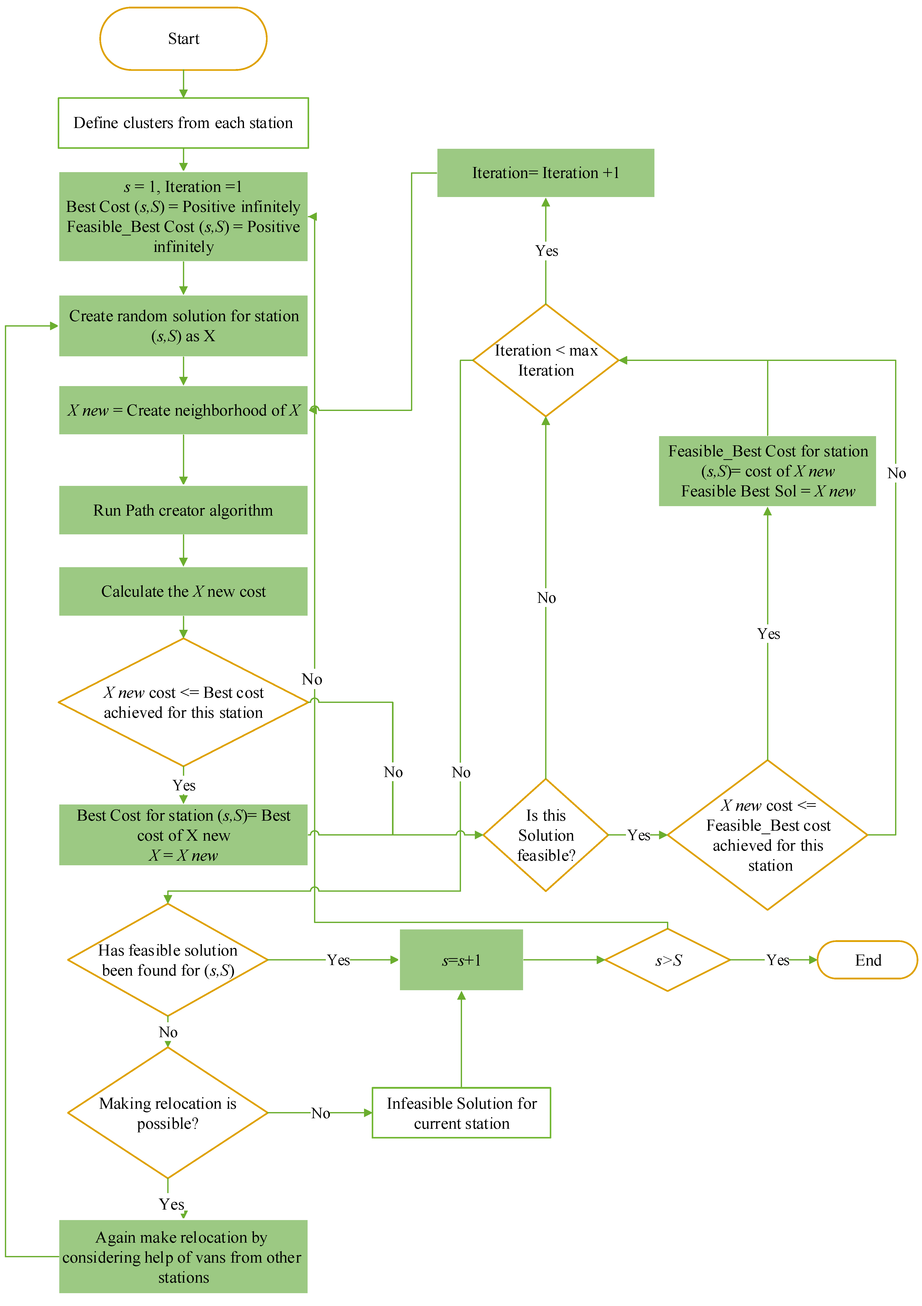
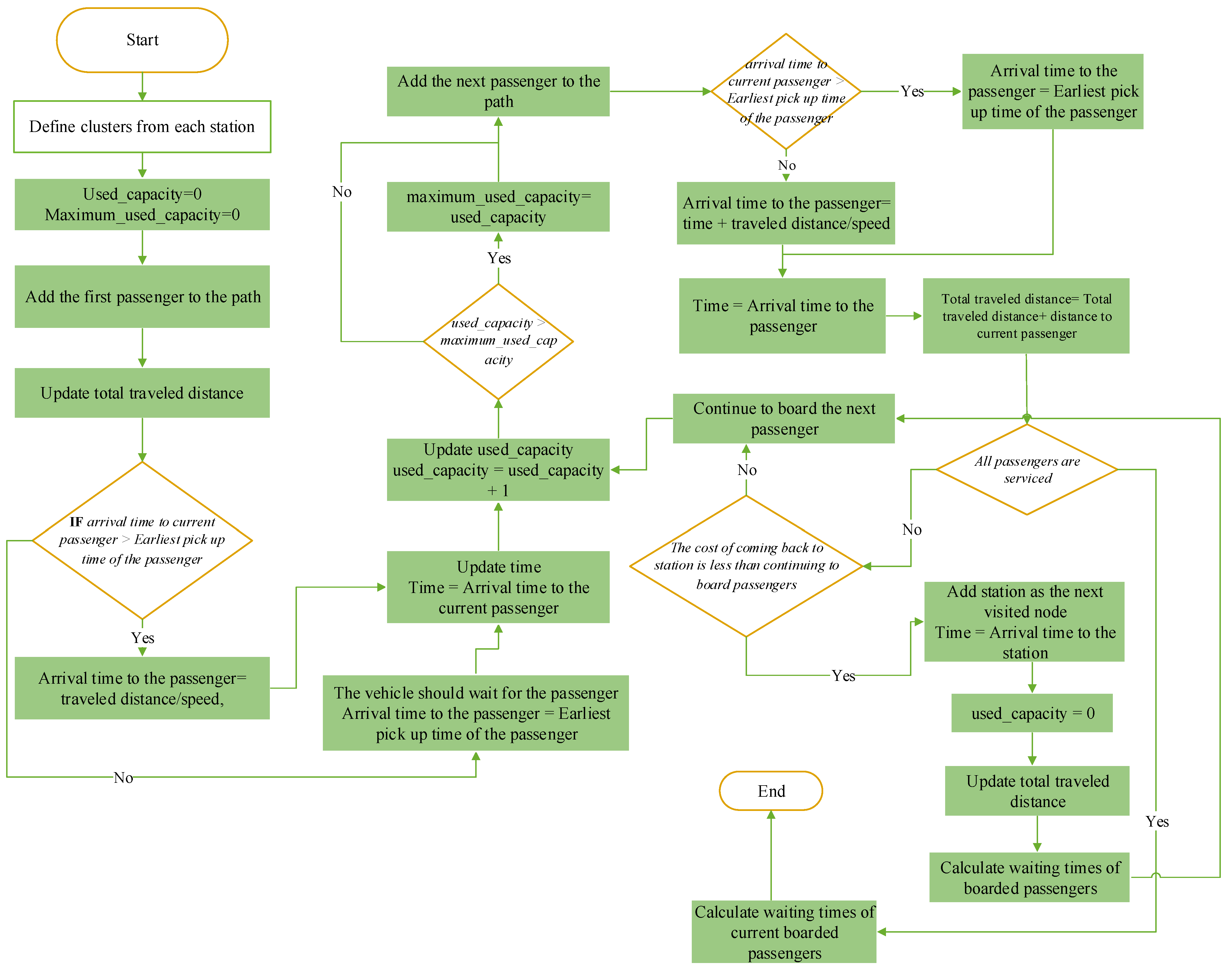
The problem consists of three main parameters: S as the number of train stations, K as the number of available feeder buses at the station s, and $I^s$ as the number of passengers in station s. In this model, $(i,j)$ represents passengers around the train stations who can be alighted/boarded to/from stations where $i\ne j=\{1,2,\dots ,I^s\}$. Each station of s has the total number of ${TV}_s$ available at the beginning. The generated routes by the algorithm can be defined as $d_{ij}^s$ which is the direct distance between passengers i and j of station s and also $d_{i0}^s$ that represents the direct distance between passenger i and station s. $R{T}_i^s$ is defined as the requested time of passenger i at station s. The speed of vehicles is defined by the speed parameter and capacity by the parameter of C. The following is the mathematical formulation. The parameter $C_T$ represents the time value of passengers per hour, and $C_O$ represents the unit operating cost of vehicles per kilometer.

Objective Function:

$$z=\min \sum _s\sum _{i=1}^{I^s}{C}_T·W{T}_i^s+\sum _{k=1}^K{C}_O· {TotalD}_k$$

(1)

Variables:

$$v_k^s=\left\{\begin{array}{c}1 \mathrm{vehicle} k \mathrm{is} \mathrm{used} \mathrm{in} \mathrm{station} s \\ 0 \mathrm{otherwise} \end{array} \right.$$

$$y_{ik}^s=\left\{\begin{array}{c}1 \mathrm{passenger} i \mathrm{in} \mathrm{station} s \mathrm{is} \mathrm{served} \mathrm{with} \mathrm{vehicle} k \\ 0 \mathrm{otherwise} \end{array}\right.$$

$${\alpha }_{ijk}^s=\left\{\begin{array}{c}1 \mathrm{passenger} j \mathrm{is} \mathrm{served} \mathrm{right} \mathrm{after} \mathrm{passenger} i \mathrm{with} \mathrm{vehicle} k (\mathrm{station} s)\\ 0 \mathrm{otherwise} \end{array}\right.$$

$$D_{ik}^s=\mathrm{d}\mathrm{i}\mathrm{s}\mathrm{t}\mathrm{a}\mathrm{n}\mathrm{c}\mathrm{e} \mathrm{t}\mathrm{r}\mathrm{a}\mathrm{v}\mathrm{e}\mathrm{l}\mathrm{e}\mathrm{d} \mathrm{u}\mathrm{p} \mathrm{t}\mathrm{o} \mathrm{p}\mathrm{a}\mathrm{s}\mathrm{s}\mathrm{e}\mathrm{n}\mathrm{g}\mathrm{e}\mathrm{r} i \mathrm{a}\mathrm{t} \mathrm{s}\mathrm{t}\mathrm{a}\mathrm{t}\mathrm{i}\mathrm{o}\mathrm{n} s \mathrm{b}\mathrm{y} \mathrm{v}\mathrm{e}\mathrm{h}\mathrm{i}\mathrm{c}\mathrm{l}\mathrm{e} k$$

$$Total{D}_k=\mathrm{t}\mathrm{o}\mathrm{t}\mathrm{a}\mathrm{l} \mathrm{d}\mathrm{i}\mathrm{s}\mathrm{t}\mathrm{a}\mathrm{n}\mathrm{c}\mathrm{e} \mathrm{t}\mathrm{r}\mathrm{a}\mathrm{v}\mathrm{e}\mathrm{l}\mathrm{e}\mathrm{d} \mathrm{b}\mathrm{y} \mathrm{v}\mathrm{e}\mathrm{h}\mathrm{i}\mathrm{c}\mathrm{l}\mathrm{e} k$$

$$A{T}_i^s=\mathrm{p}\mathrm{i}\mathrm{c}\mathrm{k} \mathrm{u}\mathrm{p} \mathrm{t}\mathrm{i}\mathrm{m}\mathrm{e} \mathrm{o}\mathrm{f} \mathrm{p}\mathrm{a}\mathrm{s}\mathrm{s}\mathrm{e}\mathrm{n}\mathrm{g}\mathrm{e}\mathrm{r} i \mathrm{i}\mathrm{n} \mathrm{s}\mathrm{t}\mathrm{a}\mathrm{t}\mathrm{i}\mathrm{o}\mathrm{n} s$$

$$C{T}_i^s=\mathrm{a}\mathrm{r}\mathrm{r}\mathrm{i}\mathrm{v}\mathrm{a}\mathrm{l} \mathrm{t}\mathrm{i}\mathrm{m}\mathrm{e} \mathrm{o}\mathrm{f} \mathrm{p}\mathrm{a}\mathrm{s}\mathrm{s}\mathrm{e}\mathrm{n}\mathrm{g}\mathrm{e}\mathrm{r} i \mathrm{t}\mathrm{o} \mathrm{s}\mathrm{t}\mathrm{a}\mathrm{t}\mathrm{i}\mathrm{o}\mathrm{n} s$$

$$W{T}_i^s=\mathrm{i}\mathrm{n} \mathrm{v}\mathrm{e}\mathrm{h}\mathrm{i}\mathrm{c}\mathrm{l}\mathrm{e} \mathrm{t}\mathrm{r}\mathrm{a}\mathrm{v}\mathrm{e}\mathrm{l} \mathrm{t}\mathrm{i}\mathrm{m}\mathrm{e} \mathrm{o}\mathrm{f} \mathrm{p}\mathrm{a}\mathrm{s}\mathrm{s}\mathrm{e}\mathrm{n}\mathrm{g}\mathrm{e}\mathrm{r} i \mathrm{o}\mathrm{f} \mathrm{s}\mathrm{t}\mathrm{a}\mathrm{t}\mathrm{i}\mathrm{o}\mathrm{n} s$$

$$U{C}_i^s=\mathrm{u}\mathrm{s}\mathrm{e}\mathrm{d} \mathrm{c}\mathrm{a}\mathrm{p}\mathrm{a}\mathrm{c}\mathrm{i}\mathrm{t}\mathrm{y} \mathrm{o}\mathrm{f} \mathrm{v}\mathrm{e}\mathrm{h}\mathrm{i}\mathrm{c}\mathrm{l}\mathrm{e} \mathrm{a}\mathrm{f}\mathrm{t}\mathrm{e}\mathrm{r} \mathrm{p}\mathrm{i}\mathrm{c}\mathrm{k}\mathrm{i}\mathrm{n}\mathrm{g} \mathrm{u}\mathrm{p} \mathrm{p}\mathrm{a}\mathrm{s}\mathrm{s}\mathrm{e}\mathrm{n}\mathrm{g}\mathrm{e}\mathrm{r} i \mathrm{o}\mathrm{f} \mathrm{s}\mathrm{t}\mathrm{a}\mathrm{t}\mathrm{i}\mathrm{o}\mathrm{n} s$$

$${\mathrm{R}\mathrm{V}}_{s{s}^{\prime }}=\mathrm{n}\mathrm{u}\mathrm{m}\mathrm{b}\mathrm{e}\mathrm{r} \mathrm{o}\mathrm{f} \mathrm{r}\mathrm{e}\mathrm{l}\mathrm{o}\mathrm{c}\mathrm{a}\mathrm{t}\mathrm{e}\mathrm{d} \mathrm{v}\mathrm{e}\mathrm{h}\mathrm{i}\mathrm{c}\mathrm{l}\mathrm{e}\mathrm{s} \mathrm{f}\mathrm{r}\mathrm{o}\mathrm{m} \mathrm{s}\mathrm{t}\mathrm{a}\mathrm{t}\mathrm{i}\mathrm{o}\mathrm{n} s \mathrm{t}\mathrm{o} s$$

$$n_{ik}^s=\mathrm{p}\mathrm{a}\mathrm{s}\mathrm{s}\mathrm{e}\mathrm{n}\mathrm{g}\mathrm{e}\mathrm{r} i \mathrm{o}\mathrm{f} \mathrm{s}\mathrm{t}\mathrm{a}\mathrm{t}\mathrm{i}\mathrm{o}\mathrm{n} s \mathrm{i}\mathrm{s} \mathrm{s}\mathrm{e}\mathrm{r}\mathrm{v}\mathrm{e}\mathrm{d} \mathrm{w}\mathrm{i}\mathrm{t}\mathrm{h} \mathrm{v}\mathrm{e}\mathrm{h}\mathrm{i}\mathrm{c}\mathrm{l}\mathrm{e} k \mathrm{i}\mathrm{n} \mathrm{t}\mathrm{h}\mathrm{e} n_{ik}^s trip from station$$

$$T{V}_s=\mathrm{t}\mathrm{h}\mathrm{e} \mathrm{t}\mathrm{o}\mathrm{t}\mathrm{a}\mathrm{l} \mathrm{n}\mathrm{u}\mathrm{m}\mathrm{b}\mathrm{e}\mathrm{r} \mathrm{o}\mathrm{f} \mathrm{v}\mathrm{e}\mathrm{h}\mathrm{i}\mathrm{c}\mathrm{l}\mathrm{e}\mathrm{s} \mathrm{a}\mathrm{v}\mathrm{a}\mathrm{i}\mathrm{l}\mathrm{a}\mathrm{b}\mathrm{l}\mathrm{e} \mathrm{a}\mathrm{t} \mathrm{s}\mathrm{t}\mathrm{a}\mathrm{t}\mathrm{i}\mathrm{o}\mathrm{n} s \mathrm{a}\mathrm{t} \mathrm{t}\mathrm{h}\mathrm{e} \mathrm{b}\mathrm{e}\mathrm{g}\mathrm{i}\mathrm{n}\mathrm{i}\mathrm{n}\mathrm{n}\mathrm{g}$$

Constraints:

$${\sum }_{k=1}^K{y}_{ik}^s=1\hspace{1em}\hspace{1em}\hspace{1em}\hspace{1em}\hspace{1em}i=1, 2,\dots ,I^s ; \forall s$$

(2)

$${\sum }_{i=1}^I{y}_{ik}^s\le M·v_k^s\hspace{1em}\hspace{1em}\hspace{1em}\hspace{1em}\hspace{1em}\forall k; \forall s$$

(3)

$${\sum }_{\mathrm{s}=1}^S{v}_k^s\le 1\hspace{1em}\hspace{1em}\hspace{1em}\hspace{1em}\hspace{1em}\hspace{1em}\forall k$$

(4)

$${\sum }_{k=1}^K{v}_k^s\le T{V}_s+{{\sum }_{s^{\prime }\ne s} (\mathrm{R}\mathrm{V}}_{s^{\prime }s}-{\mathrm{R}\mathrm{V}}_{s{s}^{\prime }})\hspace{1em}\hspace{1em}\hspace{1em}\hspace{1em}\forall s$$

(5)

$$2·{\alpha }_{ijk}^s\le (y_{ik}^s+y_{jk}^s)\hspace{1em}\hspace{1em}\hspace{1em}\hspace{1em}i,j=1,2,\dots ,I^s;i\ne j; \forall k; \forall s$$

(6)

$${\sum }_{k=1}^K{(\alpha }_{ijk}^s+{\alpha }_{jik}^s)\le 1\hspace{1em}\hspace{1em}\hspace{1em}\hspace{1em}\hspace{1em}\hspace{1em}\hspace{1em}i,j=1,2,\dots ,I^s;i\ne j; \forall s$$

(7)

$${\sum }_{k=1}^K{\sum }_{j=1}^{I^s}{\alpha }_{ijk}^s+{\sum }_{k=1}^K{\alpha }_{i0k}^s\ge 1\hspace{1em}\hspace{1em}\hspace{1em}\hspace{1em}\hspace{1em}i=1,2,\dots ,I^s ;\forall s$$

(8)

$${\sum }_{k=1}^K{\sum }_{i=1}^I{\alpha }_{ijk}^s+{\sum }_{k=1}^K{\alpha }_{0jk}^s\ge 1\hspace{1em}\hspace{1em}\hspace{1em}j=1,2,\dots ,I^s ;\forall s$$

(9)

$$D_{jk}^s\ge D_{ik}^s-M\left(1-{\alpha }_{ijk}^s\right)+\left(1-{\alpha }_{i0k}^s\right)d_{ij}^s+{\alpha }_{i0k}^s{d}_{io}^s+{\alpha }_{0jk}^s{d}_{jo}^s\hspace{1em}\hspace{1em}\hspace{1em}\hspace{1em}\hspace{1em}i,j=1,2,\dots ,I^s;i\ne j; \forall k; \forall s$$

(10)

$$D_{ik}^s\ge d_{i0}^s{y}_{ik}^s\hspace{1em}\hspace{1em}\hspace{1em}\hspace{1em}\hspace{1em}\hspace{1em}\hspace{1em}\hspace{1em}\hspace{1em}i=1,2,\dots ,I^s, k=1,2,\dots , T{V}_s; \forall s$$

(11)

$$D_{ik}^s\ge d_{i0}^{s\prime }{y}_{ik}^s\hspace{1em}\hspace{1em}\hspace{1em}\hspace{1em}\hspace{1em}\hspace{1em}\hspace{1em}\hspace{1em}\hspace{1em}i=1,2,\dots ,I^s, k=T{V}_s+1,\dots ,T{V}_s+{{\sum }_{s^{\prime }\ne s} ;\mathrm{R}\mathrm{V}}_{s^{\prime }s};\forall s$$

(12)

$$A{T}_i^s={\sum }_{k=1}^K\frac{D_{ik}^s}{speed}\hspace{1em}\hspace{1em}\hspace{1em}\hspace{1em}\hspace{1em}\hspace{1em}\hspace{1em}\hspace{1em}\hspace{1em}\hspace{1em}\hspace{1em}\hspace{1em}\hspace{1em}\hspace{1em}\hspace{1em}\hspace{1em}\hspace{1em}\hspace{1em}i=1,2,\dots ,I^s ; \forall s$$

(13)

$$W{T}_i^s=R{T}_i^s-A{T}_i^s\hspace{1em}\hspace{1em}\hspace{1em}\hspace{1em}\hspace{1em}\hspace{1em}\hspace{1em}\hspace{1em}\hspace{1em}i=1,2,\dots ,I^s; \forall s$$

(14)

$$W{T}_i^s\le Timeratio · \frac{d_{i0}^s}{speed}\hspace{1em}\hspace{1em}\hspace{1em}\hspace{1em}\hspace{1em}\hspace{1em}\hspace{1em}\hspace{1em}\hspace{1em}\hspace{1em}\hspace{1em}\hspace{1em}\hspace{1em}\hspace{1em}\hspace{1em}\hspace{1em}\hspace{1em}\hspace{1em}i=1,2,\dots ,I^s ; \forall s$$

(15)

$${\alpha }_{ijk}^s{n}_{jk}^s\ge {\alpha }_{ijk}^s \left(n_{ik}^s+{\alpha }_{i0k}^s\right)\hspace{1em}\hspace{1em}\hspace{1em}\hspace{1em}\hspace{1em}\hspace{1em}\hspace{1em}\hspace{1em}\hspace{1em}i,j=1,2,\dots ,I^s; \forall k; \forall s$$

(16)

$$M\left|n_{ik}^s-n_{jk}^s\right|+C{T}_i^s\ge {\alpha }_{j0k}^s·y_{ik}^s·y_{jk}^s·\frac{D_{jk}^s+d_{jo}^s}{speed}\hspace{1em}\hspace{1em}\hspace{1em}\hspace{1em}\hspace{1em}\hspace{1em}\hspace{1em}\hspace{1em}i,j=1,2,\dots ,I^s; \forall k; \forall s$$

(17)

$$C{T}_i^s\le R{T}_i^s\hspace{1em}\hspace{1em}\hspace{1em}\hspace{1em}\hspace{1em}\hspace{1em}\hspace{1em}\hspace{1em}\hspace{1em}\hspace{1em}\hspace{1em}\hspace{1em}\hspace{1em}\hspace{1em}\hspace{1em}\hspace{1em}i=1,2,\dots ,I^s ; \forall s$$

(18)

$${\alpha }_{ijk}^s\left(U{C}_j^s-U{C}_i^s-1\right)+M{\alpha }_{i0k}^s\ge 0\hspace{1em}\hspace{1em}\hspace{1em}\hspace{1em}\hspace{1em}\hspace{1em}\hspace{1em}\hspace{1em}i,j=1,2,\dots ,I^s ; \forall s$$

(19)

$$U{C}_i^s\le C\hspace{1em}\hspace{1em}\hspace{1em}\hspace{1em}\hspace{1em}\hspace{1em}\hspace{1em}\hspace{1em} i=1,2,\dots ,I^s; \forall s$$

(20)

$${\mathrm{T}\mathrm{o}\mathrm{t}\mathrm{a}\mathrm{l}\mathrm{D}}_{\mathrm{k}}\ge {\sum }_{s=1}^S{(D}_{ik}^s+d_{i0}^s{y}_{ik}^s )\hspace{1em}\hspace{1em}\hspace{1em}\hspace{1em}\hspace{1em}\hspace{1em}\hspace{1em}i=1,2,\dots ,I^s ; \forall k$$

(21)

$$v_k^s=(0,1), {\alpha }_{ijk}^s=(0,1), y_{ik}^s=(0,1)$$

(22)

$$D_{ik}^s\ge 0. Total{D}_k\ge 0. A{T}_i^s\ge 0. W{T}_i^s\ge 0. U{C}_i^s\ge 0. I{C}_k^{ }\ge 0. n_{ik}^s\ge 1 and integer$$

(23)

Formula (1) is the objective function of the problem. Constraint (2) specifies that each passenger is served by exactly one vehicle in that M is a big enough number used for modeling the expression. Constraint (3) ensures that if a passenger is assigned to a vehicle, it is considered as a used vehicle. Constraint (4) ensures that each vehicle starts and ends its trip from/to a station. Equation (5) makes sure that the total number of used vehicles does not exceed the total number of available vehicles. Equations (6) and (7) define each vehicle’s path. Equations (8) and (9) make sure that each passenger is assigned to a path. (Also, zero is the index used for depot.)

Equations (10)–(12) calculate the total traveled distance up to passenger i. When having relocated vehicles, Equation (12) calculates the distance to the first passenger based on the relocated vehicle’s station. Equation (13) defines the arrival time of vehicles to passengers where speed defines the vehicle’s speed. Equation (14) calculates waiting time for passengers, and Equation (15) is an additional time ratio constraint that ensures passengers will be delivered within the required time window. Equation (16) specifies in which trip of each vehicle the passenger is picked up. Equations (17) and (18) ensure that passenger arrival time at the station is scheduled before their requested time. Constraint (18) is the cycle time constraint. Equations (19) and (20) are capacity constraints. Equation (19) ensures that if passenger j is served after passenger i in station s, the used capacity of the vehicle after picking up passenger j of station s is higher unless the vehicle comes back to the station. The total traveled distance is defined by Equation (21).

3.2. Algorithm

The DRTTW problems are combinatorial, and encountering multiple local optima is expected. This study employs the SA algorithm due to its capability to escape local optima by accepting sub-optimal solutions. Moreover, given the problem’s nature, the SA algorithm can efficiently navigate a vast solution space, offering flexibility to explore and, through iterative refinements, achieve a near-optimal solution within a reasonable timeframe. The SA algorithm starts with a random solution and an initial high temperature. As iterations progress, the temperature decreases according to a cooling schedule. Convergence is determined by a set number of iterations and when temperature drops below a threshold. A cooling rate of 0.99 was chosen to ensure a gradual reduction in temperature, allowing the algorithm an extended exploration period before becoming more exploitative. Furthermore, the initial temperature was set at a sufficiently high value, enabling the algorithm to explore a broad spectrum of solutions from the outset. This strategy allows the SA algorithm to start with a more explorative approach, accepting even some suboptimal solutions to ensure it does not become trapped in local minima.

When there are many passengers with different arrival time requests, meeting the exact train may not be so necessary, which means feeder buses can deliver the passengers any time as long as it is no later than their requested time. Although feeder buses can deliver passengers any time before the requested time, waiting time due to the early arrival should be included in the total travel time, and the maximum travel time ratio constraint should be met. Also, passengers cannot be picked up before their available departure time. To generate the initial solution, a random permutation with the length of “number of passengers at the related station plus number of feeder buses minus one” is produced. Then, depending on the location of greater numbers, the assignment of passengers to feeder buses is determined. For instance, in the presence of two feeder buses and 10 passengers, a permutation with length 11 is produced. Suppose that the generated permutation is as follows: Path = [10, 1, 3, 4, 8, 11, 2, 9, 5, 7, 6]. The path creator section was included in the model as a sub-algorithm.

The next step is to define the routes of feeder buses. The feeder bus first picks up the first assigned passenger and continues picking up the others in turn. However, it would return to the station if its capacity is full. Also, it makes a comparison and returns to the station if the cost of the trip when returning to the station is less than the cost of continuing the route and picking up the next passenger. The feeder bus can also wait for the passenger to reach the passenger’s allowed time to pick up based on the maximum acceptable time ratio. Furthermore, the feeder bus tries to return to the station before the requested times of its passengers. In each iteration, the algorithm tries to improve the solution by searching its neighborhoods. For this purpose, common swap, insertion, and reversion methods were used.

The algorithm calculates the earliest and latest possible alighting/boarding time for each passenger. The latest alighting/boarding time is simply equal to the difference between arrival/departure time request and direct travel time (arrival/departure time request-direct travel time). In this stage, the algorithm assumes the feeder bus goes directly to the station right after alighting/boarding the passenger. In the next step, a series of passengers would be assigned to each vehicle, and new variables named “updated latest alighting/boarding time” would be introduced which are the latest possible alighting/boarding time for each passenger according to the defined series of passengers. This variable helps determine what series of passengers after serving a certain series should be served. Obviously, the updated latest alighting/boarding time will be equal to the latest alighting/boarding time for the last passenger. If we indicate a series of passengers with i, then the updated latest alighting/boarding time can be expressed as

$$\begin{array}{l}\mathrm{U}\mathrm{p}\mathrm{d}\mathrm{a}\mathrm{t}\mathrm{e}\mathrm{d} \mathrm{l}\mathrm{a}\mathrm{t}\mathrm{e}\mathrm{s}\mathrm{t} \mathrm{p}\mathrm{i}\mathrm{c}\mathrm{k} \mathrm{u}\mathrm{p} \mathrm{t}\mathrm{i}\mathrm{m}\mathrm{e} \left(i\right)\\ = \mathrm{m}\mathrm{i}\mathrm{n} (\mathrm{U}\mathrm{p}\mathrm{d}\mathrm{a}\mathrm{t}\mathrm{e}\mathrm{d} \mathrm{l}\mathrm{a}\mathrm{t}\mathrm{e}\mathrm{s}\mathrm{t} \mathrm{p}\mathrm{i}\mathrm{c}\mathrm{k} \mathrm{u}\mathrm{p} \mathrm{t}\mathrm{i}\mathrm{m}\mathrm{e} (i+1)-\mathrm{d}\mathrm{i}\mathrm{r}\mathrm{e}\mathrm{c}\mathrm{t} \mathrm{t}\mathrm{r}\mathrm{a}\mathrm{v}\mathrm{e}\mathrm{l} \mathrm{t}\mathrm{i}\mathrm{m}\mathrm{e} \mathrm{f}\mathrm{r}\mathrm{o}\mathrm{m} i \mathrm{t}\mathrm{o}\\ (i+1), \mathrm{l}\mathrm{a}\mathrm{t}\mathrm{e}\mathrm{s}\mathrm{t} \mathrm{p}\mathrm{i}\mathrm{c}\mathrm{k} \mathrm{u}\mathrm{p} \mathrm{t}\mathrm{i}\mathrm{m}\mathrm{e} \left(i\right))\end{array}$$

In the previous algorithm, after assigning a series of passengers to each vehicle, the algorithm tries to make a route for each vehicle. However, in the developed algorithm, the introduced variable of updated latest alighting/boarding time decides whether vehicles return to the station or continue the trip. In this case, when the cost (both vehicle and passenger traveling costs) of going back to the station is less than continuing the trip, the vehicles return to the station only if there is a feasible solution for that. In other words, the updated latest alighting/boarding time must be bigger than the arrival/departure time. Therefore, the variable of the updated latest alighting/boarding time ensures reaching a feasible solution.

The cost of each new solution (Z’) is calculated based on the passengers’ travel time and the cost of consumed fuel. The travel time of passengers picked up at stations and getting off at destinations is equal to the destination arrival time minus feeder bus departure time. The travel time of passengers getting off at train stations is equal to the arrival time at the train station minus the arrival time of the feeder bus to passengers. To model constraints, penalties were used in the objective function. The value of the objective function (Z’) for each generated solution was calculated. Then, based on the feasibility of the solution, the hypothesized objective function (Z) was defined, in which the penalties were also added to the value of the original objective function value. The algorithm attempts to reduce the value of the hypothesized objective function. The original and hypothetical objective functions are calculated as follows:

$$\begin{gathered} Z^{\prime }=vehicle travel cost per\frac{km}{h}·Total vehicles traveled distance \\ +the value of passenger{s}^{\prime }time per hr \\ ·Total passengers in vehicle travel time \end{gathered}$$

$$\begin{gathered} Z=Z\prime ·(1+0.5· number of passengers not served in time window+5 \\ ·maximum number of passengers in excess of feeder bus capacity) \end{gathered}$$

The maximum capacity of the feeder bus was assumed to be 12, and the related constraint was considered as a penalty in the objective function. The penalty was equal to half of the maximum number of passengers in excess of feeder bus capacity. The algorithm saves the best solution and the best feasible solution (considering time ratios), and ultimately presents the best feasible solution as the final solution. The best infeasible solutions, which are unacceptable in terms of the maximum time ratio, are accepted, since the algorithm may produce a feasible solution for their neighborhoods. For this reason, the best infeasible solutions were accepted to expand the search space and reach the optimal global solution. If more buses are needed in a certain station and none of the stations have a surplus, serving all the passengers would become impossible with this number of buses. In order to validate the obtained results, the authors ran the algorithm 10 times, and the best solution was selected. The framework of the developed algorithm is shown in Figure 2 and Figure 3. This framework comprises two algorithms: Algorithm 1, which is designed to solve the model, and Algorithm 2, the developed SA path creator.

Algorithm 1: Pseudocode for the developed SA algorithm to solve the model

Step 0: Initialization:

Set s=1,   Best Cost=positive infinite,   T=T0,   alpha=0.99,   previous station help=0,   next station help=0,   vehicle (s; s: 1 to S)=4,   min vehicle(s; s: 1 to S) = 0

Step 1: Clustering: Define passenger’s cluster

Step 2: Create random solution

Considering the length of trip (number of passengers (s) +vehicles(s)-1)

Step 3: Sort the initial solution based of desired departure time of passengers for each feeder bus

set x as a random solution

Step 4: Find optimal solution:

IF It1<It1max, THEN

go to step 5, otherwise go to step 7

END IF

Step 5: IF It2< It2max, THEN

go to step 5.1, otherwise go to step 6

END IF

Step 5.1: Creating neighborhood:

set xnew = a neighborhood of x

Step 5.2: Run Path Creator Algorithm

Step 5.3: IF best cost for x< best cost for xnew, THEN

set x=xnew and go to step 5.6, otherwise go to step 5.4

END IF

Step 5.4: p= exp-(cost xnew – cost x)/T·Cost x

Step 5.5: Accept x= xnew by p -probability and reject- and x= xnew by (1-p) and go to step 5.6

Step 5.6: Cost calculation for xnew

Step 5.7: IF best cost for xnew > best cost, THEN

set bestsol= xnew

END IF

Step 5.8: IF xnew is feasible (considering time ratio), and best cost for xnew > feasible_best cost, THEN

set feasible_bestsol= xnew

END IF

Step 5.9: Reducing the temperature:

set T = alpha·T0 (0<alpha<1)

Step 5.10: set It2=It2+1 and go to step 5

Step 6: Set It1=It1+1 and go to step 4

Step 7: IF feasible_bestsol is empty, THEN

min vehicle (s)= vehicle (s)+1 and go to step 8, otherwise go to step 15

END IF

Step 8: Calculate the following proportion for stations s-1 and s+1: number of passengers (s)/vehicle(s)

Step 9: IF s-1 exists and vehicle (s-1)> min vehicle (s-1), THEN

go to step 10, otherwise go to step 12

END IF

Step 10: IF proportion for station s is $\le$ the proportion for station s+1 or vehicle (s+1) $\le$ min vehicle (s+1)

go to step 11, otherwise go to step 12

END IF

Step 11: Set previous station help (s)= previous station help (s)+1 and vehicle (s-1) = vehicle (s-1)-1, s=s-1, and go to step 2

Step 12: IF s+1 exists and vehicle (s+1)> min vehicle (s+1) THEN

go to step 13, otherwise go to step 14

END IF

Step 13: Set next station help (s)= next station help(s)+1 and vehicle (s+1) = vehicle (s+1)-1 and go to step 2

Step 14: Show “The problem is not feasible; more vehicles is needed”

Step 15: IF s<S, THEN

set s=s+1 and go to step 2, otherwise go to step 16

END IF

Step 17: END

Algorithm 2: Pseudocode for the developed SA path creator algorithm

Step 0: Initialization:

Set used_capacity=0, maximum_used_capacity =0, c

Step 1: Calculate updated latest pickup time of passengers based on the sequence of passengers

Step 2: Add the first passenger to the path

Step 3: Update total traveled distance

Total traveled distance= Distance to current passenger

Step 4: IFarrival time to current passenger > Earliest pick up time of the passenger

Arrival time to the passenger= traveled distance/speed,

else

The vehicle should wait for the passenger

Arrival time to the passenger = Earliest pick up time of the passenger

END IF

Step 5: Update time

Time = Arrival time to the current passenger

Step 6: Update used_capacity

used_capacity = used_capacity + 1

Step 7: Update maximum_used_capacity

IF used_capacity > maximum_used_capacity

maximum_used_capacity= used_capacity

END IF

Step 8: For the next passengers:

Step 7.1: Add the next passenger to the path

Step 7.2: IF arrival time to current passenger > Earliest pick up time of the passenger THEN go to step 9, otherwise go to step 10

Step 9:Arrival time to the passenger= time + traveled distance/speed

Time = Arrival time to the passenger

Step 10: The vehicle should wait for the passenger

Arrival time to the passenger = Earliest pick up time of the passenger

Time = Arrival time to the passenger

Step 11:Total traveled distance= Total traveled distance+ distance to current passenger

Step 12:Check to see if the cost of coming back to the station is better than continuing to board passengers (for the last passenger)

IF the cost of coming back to station is less than continuing to board passengers THEN go to step 13, otherwise go to step 15 Step 13: Check to see coming back to station does not makes the path infeasible

IF in case of coming back to the station the updated latest pick up time of the next passenger is accepted THEN go to step 14, otherwise go to step 15

Step 14:Add station as the next visited node

Step 14.1: Time = Arrival time to the station

Step 14.2: used_capacity = 0

Step 14.3: Update total traveled distance

Step 14.4: Calculate waiting times of boarded passengers

Step 15: Accept continue to board the next passenger

Step 15.1: Update used_capacity

used_capacity = used_capacity + 1

Step 15.2: Update maximum_used_capacity

IF used_capacity > maximum_used_capacity

maximum_used_capacity= used_capacity

END IF

Step 15.3: go to step 8

Step 16: Calculate waiting times of current boarded passengers

Step 17: END

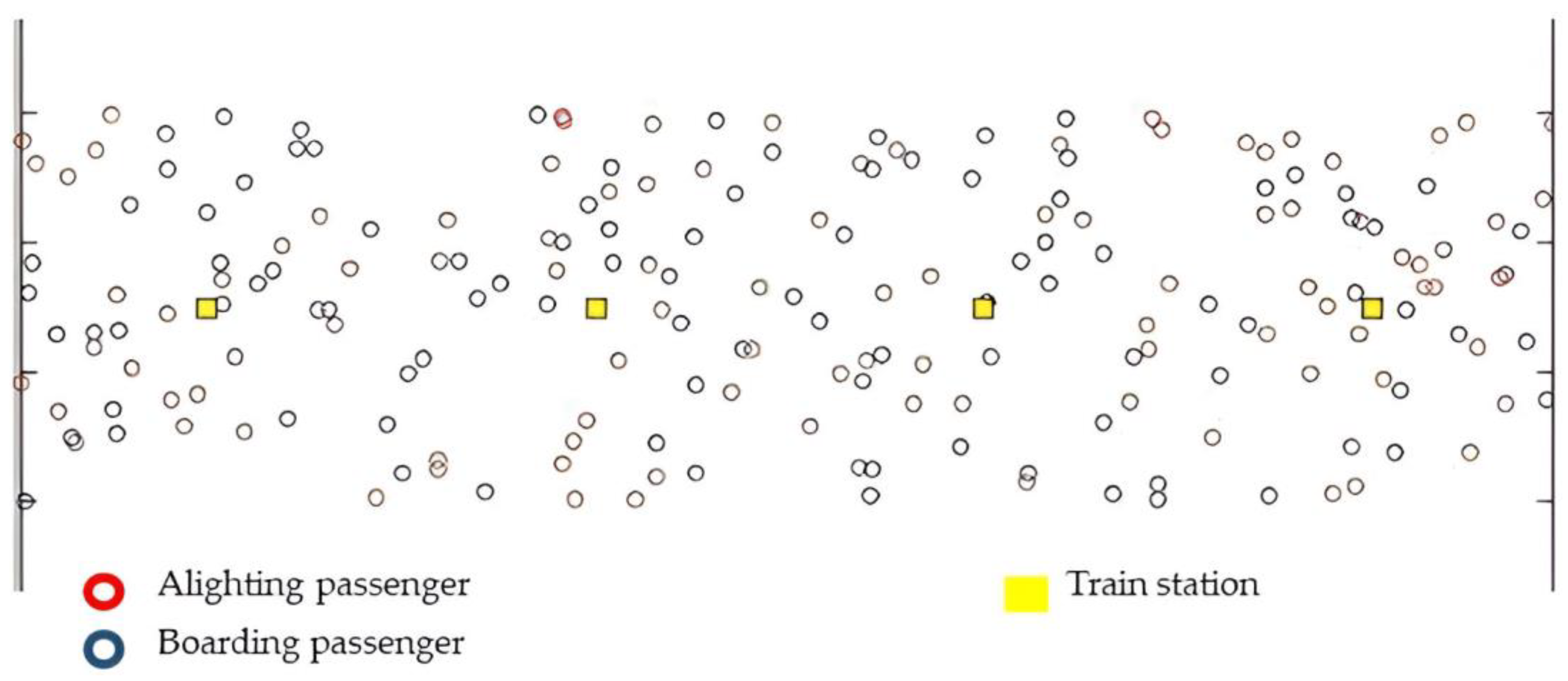
4. Hypothetical Network

A hypothetical rail transit line that has four stations fitted to urban and suburban conditions was developed to examine and evaluate the efficiency of the algorithm. In this example, the headway of the train is assumed to be 5 min, and the travel time between two stations is assumed to be 2 min. Three buses are assigned to each station initially, and a total of 12 buses are available in the model. Passengers’ boarding and alighting times at the nodes and the stations were waived in this study. Figure 4 shows the geographical distribution of the passengers in the hypothetical network where the circle points represent passengers, and the four yellow boxes are stations.

Table 2. Passenger information for each station and each train.

Train/ Station	Station A			Station B			Station C			Station D			Average Total Direct Travel Distance (km)
	B 1	A	Average Direct Travel Distance (km) 2	B	A	Average Direct Travel Distance (km)	B	A	Average Direct Travel Distance (km)	B	A	Average Direct Travel Distance (km)
Bus set 1	1	1	1.01	1	1	1.01	1	1	1.01	1	1	1.01	1.01
Bus set 2	3	1	1.01	4	2	2.02	6	1	1.01	2	3	3.03	1.77
Bus set 3	4	4	4.04	3	3	3.03	4	3	3.03	3	2	2.02	3.03
Bus set 4	3	2	2.02	2	2	2.02	4	2	2.02	2	2	2.02	2.02
Bus set 5	6	3	3.03	1	3	3.03	3	2	2.02	2	2	2.02	2.52
Bus set 6	2	3	3.03	3	1	1.01	3	3	3.03	2	2	2.02	2.27
Bus set 7	4	3	3.03	3	3	3.03	3	2	2.02	1	2	2.02	2.52
Bus set 8	3	2	2.02	2	2	2.02	4	2	2.02	1	7	7.07	3.28
Bus set 9	1	3	3.03	6	1	1.01	5	3	3.03	2	3	3.03	2.52
Bus set 10	3	3	3.03	1	1	1.01	2	1	1.01	1	1	1.01	1.51
Bus set 11	6	4	4.04	4	4	4.04	4	2	2.02	2	3	3.03	3.28
Bus set 12	0	1	1.01	0	7	7.07	1	3	3.03	1	3	3.03	3.53
Bus set 13	0	2	2.02	0	3	3.03	0	3	3.03	1	1	1.01	2.27

¹ Boarding/alighting passengers (prs). ² Average direct travel distance in kilometers (km).

represents the number of boarding and alighting (B/A) passengers for each station and each train. The origins and the destinations of the boarding and alighting passengers are randomly generated around the rail line for four trains. In this paper, it is assumed that the average speed for feeder buses is 30 km/h and for trains is 60 km/h; each bus has a 12-passenger capacity, and the distance between stations is 1 km. The duration time for the model was considered as one hour; therefore, there would be 12 train sets according to the 5 min headway of trains. The travel time monetary value for each passenger was assumed as USD 20 per hour, and USD 5 per kilometer for vehicles was used as the feeder bus operating costs. The inputs of the example are passenger locations, passenger schedules, headway for arrival trains, vehicle speed, trains’ schedules, stations’ coordination, and velocity of trains. Accordingly, the outputs would be passengers’ travel time, vehicles’ traveled distance, assigned buses in each station in each time window, relocated buses, and routes.

5. Results and Analysis

The proposed SA started with the initializing of inputs and clustering of the passengers. It is important in this algorithm that the cost calculation process includes three parameters: without relocation to other stations, considering relocated bus(es) from the previous station, and considering relocated bus(es) from the following station.

Table 3. The results of computations for the model.

Station	Total Vehicle Traveled Distance (km)	Total Passenger Travel Time (hour)	Average Passenger Distance Traveled to each Station (km)	Average Total Passenger Average Distance Traveled (km)	Average Total Passenger Travel Cost (USD)	Average Total Bus Operating Cost (USD)
#1	67.69	3.09	1.66	1.74	24.81	21.33
#2	48.31	2.51	1.47
#3	70.92	3.08	1.90
#4	64.34	3.13	1.50

shows the results of the computations for the model. Figure 5 shows the results of the feeder bus movements including relocation of the buses for stations. In this figure, the travel path is indicated by arrows, with the arrow’s beginning signifying the starting point and its end denoting the end of the trip. Each color corresponds to a distinct bus. As shown, the blue and red buses are relocated to another station.

6. Discussion and Conclusions

This study aimed to create a routing algorithm for a demand-responsive feeder transit system aligned with short headway mass transit. Building on a previous model [8] designed for long headway trunk lines in less dense areas, the new routing accommodates more frequent train services.

Developing a similar algorithm for use in more congested urban areas motivated the authors to develop a new specialized algorithm where the headway of metro trains is much shorter. Therefore, a 5 min headway was considered in the hypothetical network of this study. When the headway of the rail service is long enough for the feeder buses to come back by the next train, then the feeder network algorithm is rather easy because the maximum feeder service cycle time is determined by the rail headway, and matching between feeder buses and the trains is not necessary. However, if the headway of the rail service is not long enough for the feeder buses to return before the next train, then the algorithm should find not only matching between passengers and feeder buses but also matching between feeder buses and trains because the bus can deliver passengers any time as long as it is no later than their requested time. This makes fundamental changes in the algorithm.

In this study, a simulated annealing (SA) algorithm was developed for flexible feeder bus routing on short trunk lines, taking into account the relocation of buses across multiple stations. The objective function of the model incorporated both operating costs and passenger travel expenses. The proposed algorithm effectively managed bus relocations when optimal routing was infeasible due to bus availability constraints at specific stations.

For future research, it is recommended to develop a feeder bus routing algorithm for trains with equivalent short headways, including temporary stops for feeder buses. Furthermore, incorporating composite heuristics for the larger and real networks and exploring the use of more advanced metaheuristics within the algorithm are suggested.

References

1. Shaheen, S.; Cohen, A. Shared ride services in North America: Definitions, impacts, and the future of pooling. Transp. Rev. 2019, 39, 427–442. [Google Scholar] [CrossRef]
2. Velaga, N.R.; Rotstein, N.D.; Oren, N.; Nelson, J.D.; Norman, T.J.; Wright, S. Development of an integrated flexible transport systems platform for rural areas using argumentation theory. Res. Transp. Bus. Manag. 2012, 3, 62–70. [Google Scholar] [CrossRef]
3. Li, X.; Quadrifoglio, L. Feeder transit services: Choosing between fixed and demand responsive policy. Transp. Res. Part C Emerg. Technol. 2010, 18, 770–780. [Google Scholar] [CrossRef]
4. Mulley, C.; Nelson, J.D. Flexible transport services: A new market opportunity for public transport. Res. Transp. Econ. 2009, 25, 39–45. [Google Scholar] [CrossRef]
5. Archetti, C.; Speranza, M.G.; Weyland, D. A simulation study of an on-demand transportation system. Int. Trans. Oper. Res. 2018, 25, 1137–1161. [Google Scholar] [CrossRef]
6. Mendes, R.; Wanner, E.; Martins, F.; Sarubbi, J. Dimensionality Reduction Approach for Many-Objective Vehicle Routing Problem with Demand Responsive Transport. In Proceedings of the International Conference on Evolutionary Multi-Criterion Optimization, Münster, Germany, 19–22 March 2017; Springer: Berlin/Heidelberg, Germany, 2017. [Google Scholar]
7. Fan, L.; Mumford, C.L. A metaheuristic approach to the urban transit routing problem. J. Heuristics 2010, 16, 353–372. [Google Scholar] [CrossRef]
8. Lee, Y.-J.; Meskar, M.; Nickkar, A.; Sahebi, S. Development of an Algorithm for Optimal Demand Responsive Relocatable Feeder Transit Networks Serving Multiple Trains and Stations. Urban Rail Transit 2019, 5, 186–201. [Google Scholar] [CrossRef]
9. Berger, T.; Sallez, Y.; Raileanu, S.; Tahon, C.; Trentesaux, D.; Borangiu, T. Personal Rapid Transit in an open-control framework. Comput. Ind. Eng. 2011, 61, 300–312. [Google Scholar] [CrossRef]
10. Lees-Miller, J.; Hammersley, J.; Wilson, R. Theoretical Maximum Capacity as Benchmark for Empty Vehicle Redistribution in Personal Rapid Transit. Transp. Res. Rec. J. Transp. Res. Board 2010, 2146, 76–83. [Google Scholar] [CrossRef]
11. Wang, H. Routing and Scheduling for a Last-Mile Transportation System. Transp. Sci. 2017, 53, 1–17. [Google Scholar] [CrossRef]
12. Raghunathan, A.U.; Bergman, D.; Hooker, J.N.; Serra, T.; Kobori, S. The Integrated Last-Mile Transportation Problem (ILMTP). In Proceedings of the 28th International Conference on Automated Planning and Scheduling (ICAPS), Delft, The Netherlands, 24–29 June 2018. [Google Scholar]
13. Ma, T.-Y.; Rasulkhani, S.; Chow, J.Y.J.; Klein, S. A dynamic ridesharing dispatch and idle vehicle repositioning strategy with integrated transit transfers. Transp. Res. Part E Logist. Transp. Rev. 2019, 128, 417–442. [Google Scholar] [CrossRef]
14. Arbex, R.O.; da Cunha, C.B. Efficient transit network design and frequencies setting multi-objective optimization by alternating objective genetic algorithm. Transp. Res. Part B Methodol. 2015, 81, 355–376. [Google Scholar] [CrossRef]
15. Diana, M.; Dessouky, M.M.; Xia, N. A model for the fleet sizing of demand responsive transportation services with time windows. Transp. Res. Part B Methodol. 2006, 40, 651–666. [Google Scholar] [CrossRef]
16. Horn, M.E. Fleet scheduling and dispatching for demand-responsive passenger services. Transp. Res. Part C Emerg. Technol. 2002, 10, 35–63. [Google Scholar] [CrossRef]
17. Mahéo, A.; Kilby, P.; Van Hentenryck, P. Benders decomposition for the design of a hub and shuttle public transit system. Transp. Sci. 2017, 53, 77–88. [Google Scholar] [CrossRef]
18. Pternea, M.; Kepaptsoglou, K.; Karlaftis, M.G. Sustainable urban transit network design. Transp. Res. Part A Policy Pract. 2015, 77, 276–291. [Google Scholar] [CrossRef]
19. Sloman, L.; Hendy, P. A New Approach to Rural Public Transport; Commission for Integrated Transport (CfIT): London, UK, 2008. [Google Scholar]
20. Psaraftis, H.N. A Dynamic Programming Solution to the Single Vehicle Many-to-Many Immediate Request Dial-a-Ride Problem. Transp. Sci. 1980, 14, 130–154. [Google Scholar] [CrossRef]
21. Sexton, T.R.; Bodin, L.D. Optimizing Single Vehicle Many-to-Many Operations with Desired Delivery Times: II. Routing. Transp. Sci. 1985, 19, 411–435. [Google Scholar] [CrossRef]
22. Garaix, T.; Artigues, C.; Feillet, D.; Josselin, D. Vehicle routing problems with alternative paths: An application to on-demand transportation. Eur. J. Oper. Res. 2010, 204, 62–75. [Google Scholar] [CrossRef]
23. Garaix, T.; Artigues, C.; Feillet, D.; Josselin, D. Optimization of occupancy rate in dial-a-ride problems via linear fractional column generation. Comput. Oper. Res. 2011, 38, 1435–1442. [Google Scholar] [CrossRef]
24. Attanasio, A.; Cordeau, J.-F.; Ghiani, G.; Laporte, G. Parallel Tabu search heuristics for the dynamic multi-vehicle dial-a-ride problem. Parallel Comput. 2004, 30, 377–387. [Google Scholar] [CrossRef]
25. Cordeau, J.-F.; Laporte, G. A tabu search heuristic for the static multi-vehicle dial-a-ride problem. Transp. Res. Part B Methodol. 2003, 37, 579–594. [Google Scholar] [CrossRef]
26. Teodorovic, D.; Radivojevic, G. A fuzzy logic approach to dynamic Dial-A-Ride problem. Fuzzy Sets Syst. 2000, 116, 23–33. [Google Scholar] [CrossRef]
27. Cordeau, J.-F. A Branch-and-Cut Algorithm for the Dial-a-Ride Problem. Oper. Res. 2006, 54, 573–586. [Google Scholar] [CrossRef]
28. Gupta, A.; Hajiaghayi, M.; Nagarajan, V.; Ravi, R. Dial a Ride from k-Forest; Springer: Berlin/Heidelberg, Germany, 2007. [Google Scholar]
29. Okulewicz, M.; Mańdziuk, J. A metaheuristic approach to solve Dynamic Vehicle Routing Problem in continuous search space. Swarm Evol. Comput. 2019, 48, 44–61. [Google Scholar] [CrossRef]
30. Ozbaygin, G.; Savelsbergh, M. An iterative re-optimization framework for the dynamic vehicle routing problem with roaming delivery locations. Transp. Res. Part B Methodol. 2019, 128, 207–235. [Google Scholar] [CrossRef]
31. Respen, J.; Zufferey, N.; Potvin, J.-Y. Impact of vehicle tracking on a routing problem with dynamic travel times. RAIRO-Oper. Res. 2019, 53, 401–414. [Google Scholar] [CrossRef]
32. Vansteenwegen, P.; Melis, L.; Aktaş, D.; Montenegro, B.D.G.; Sartori Vieira, F.; Sörensen, K. A survey on demand-responsive public bus systems. Transp. Res. Part C Emerg. Technol. 2022, 137, 103573. [Google Scholar] [CrossRef]
33. Molenbruch, Y.; Braekers, K.; Hirsch, P.; Oberscheider, M. Analyzing the benefits of an integrated mobility system using a matheuristic routing algorithm. Eur. J. Oper. Res. 2021, 290, 81–98. [Google Scholar] [CrossRef]
34. Pavone, M.; Frazzoli, E.; Bullo, F. Adaptive and Distributed Algorithms for Vehicle Routing in a Stochastic and Dynamic Environment. IEEE Trans. Autom. Control 2011, 56, 1259–1274. [Google Scholar] [CrossRef]
35. Furtado, M.G.S.; Munari, P.; Morabito, R. Pickup and delivery problem with time windows: A new compact two-index formulation. Oper. Res. Lett. 2017, 45, 334–341. [Google Scholar] [CrossRef]
36. Ayadi, M.; Chabchoub, H.; Yassine, A. A new mathematical formulation for the static demand responsive transport problem. Int. J. Oper. Res. 2017, 29, 495–507. [Google Scholar] [CrossRef]
37. Osaba, E.; Diaz, F.; Onieva, E.; López-García, P.; Carballedo, R.; Perallos, A. Parallel Meta-Heuristic for Solving a Multiple Asymmetric Traveling Salesman Problem with Simulateneous Pickup and Delivery Modeling Demand Responsive Transport Problems; Springer International Publishing: Cham, Switzerland, 2015. [Google Scholar]
38. Van Engelen, M.; Cats, O.; Post, H.; Aardal, K. Demand-Anticipatory Flexible Public Transport Service. In Proceedings of the Transportation Research Board 97th Annual Meeting Transportation Research Board, Washington DC, USA, 7–11 January 2018. [Google Scholar]
39. Paradiso, R.; Roberti, R.; Laganá, D.; Dullaert, W. An Exact Solution Framework for Multitrip Vehicle-Routing Problems with Time Windows. Oper. Res. 2020, 68, 180–198. [Google Scholar] [CrossRef]
40. Dou, X.; Gong, X.; Guo, X.; Tao, T. Coordination of Feeder Bus Schedule with Train Service at Integrated Transport Hubs. Transp. Res. Rec. J. Transp. Res. Board 2017, 2648, 103–110. [Google Scholar] [CrossRef]
41. Lee, Y.-J.; Nickkar, A. Optimal Automated Demand Responsive Feeder Transit Operation and Its Impact; Urban Mobility & Equity Center, Morgan State University: Baltimore, MD, USA, 2018; pp. 16–27. [Google Scholar]
42. Yang, Y.; Jiang, X.; Fan, W.; Yan, Y.; Xia, L. Schedule Coordination Design in a Trunk-Feeder Transit Corridor with Spatially Heterogeneous Demand. IEEE Access 2020, 8, 96391–96403. [Google Scholar] [CrossRef]
43. Kuah, G.K.; Perl, J. The feeder-bus network-design problem. J. Oper. Res. Soc. 1989, 40, 751–767. [Google Scholar] [CrossRef]
44. Zhao, J.; Sun, S.; Cats, O. Joint optimisation of regular and demand-responsive transit services. Transp. A Transp. Sci. 2023, 19, 1987580. [Google Scholar] [CrossRef]
Figure 1. Conceptual operation of the proposed demand-responsive feeder transit service.
Algorithms 16 00506 g001
Figure 2. The developed SA algorithm to solve the model.
Algorithms 16 00506 g002
Figure 3. The path creator algorithm.
Algorithms 16 00506 g003
Figure 4. Geographical distributions of the passengers.
Algorithms 16 00506 g004
Figure 5. Illustration for the feeder bus schedules and movements.
Algorithms 16 00506 g005