Article

The Importance of Modeling Path Choice Behavior in the Vehicle Routing Problem

Dipartimento di Ingegneria dell’Informazione, Università degli Studi Mediterranea di Reggio Calabria, delle Infrastrutture e dell’Energia Sostenibile, 89122 Reggio Calabria, Italy
Algorithms 2023, 16(1), 47; https://doi.org/10.3390/a16010047
Submission received: 30 November 2022 / Revised: 30 December 2022 / Accepted: 4 January 2023 / Published: 10 January 2023
(This article belongs to the Special Issue Optimization for Vehicle Routing Problems)

Abstract

:
Given two pick-up and delivery points, the best path chosen does not necessarily follow the criteria of minimum travel time or generalized minimum cost evaluated with a deterministic approach. Given a criterion, the perceived cost is not deterministic for many reasons (congestion, incomplete information on the state of the system, inexact prediction of the system state, etc.). The same consideration applies to the best-chosen route, assuming that the route is an ordered list of network nodes to visit. The paths and routes perceived and chosen (drivers or companies) could follow different criteria (i.e., minizmum congested travel time for the path and minimum monetary cost for the route). In this context, the paths chosen between two pick-up and delivery points, studied with the path choice problem (PCP), influence the best route, studied with the vehicle routing problem (VRP). This paper reports some considerations on the importance of modelling the path choice behavior in the VRP; the influence of the PCP on the VRP is studied. The considerations are supported by a numerical example in a small network in which the results obtained by adopting the deterministic or probabilistic models for the PCP are compared. To validate the reported thesis, the models are applied in a small test system, and it allows the reader to follow the numerical results step by step.

1. Introduction

The transport system has an important role within smart cities (SC) and intelligent transport systems (ITS). Further details are given in Section 2. The introduction of increasingly advanced technologies and the development of smart cities has made the transport system increasingly important, and it is one of the three pillars of the smart city. Of fundamental importance is the construction of adequate reliable mathematical models to be used for the design and management of transport systems.
In this context, the problem of the path choice between a pair of points and the influence of the best sequence of paths between serial pairs of points in a transport system are studied. It can support the decision-takers and the analysts for the transport system design and management.
In this paper, considering a transport network model, the following definitions are assumed:
(1)
A path is a set of consecutive and loopless transport network links connecting two consecutive nodes of the route; between two nodes, one or more paths can be perceived; the path choice is studied with the path choice problem (PCP);
(2)
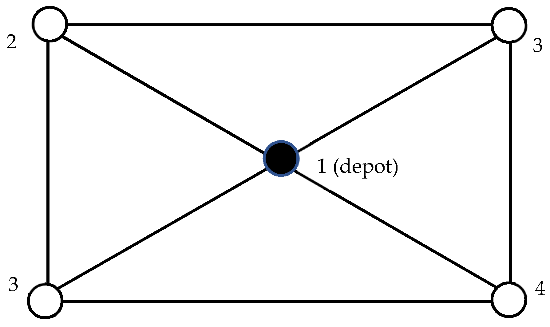
A route is an ordered list of network nodes (in the case of freight for pick-up and delivery activities) to be visited following paths; the optimal routes are studied with the vehicle routing problem (VRP).
The general objective of this work is to investigate the role of PCP in the VRP, in the transport network, in order to identify the influence of user choice. The specific objective concerns the study of the importance of the correct path choice modeling for the evaluation of the optimal routing configuration. Proper modeling and optimization can help the system manager in the context of transport system planning activities for the optimization of the entire transport system from the point of view of users, citizens and companies (i.e., freight distribution for the delivery company, dial and ride for the passenger companies), for the optimization of the routes and paths. The method proposed can support decision-takers and for this reason, this paper proposes the problem at a methodological level. This paper does not have a specific objective concerning the study of the algorithms to be adopted for the solution of the PCP and the VRP.
The literature on PCP and VRP solution models and algorithms is very extensive. Considering the objectives of this paper, some references are reported in each research area and the references reported are not exhaustive. A classification of the reported state of the art is reported in Figure 1. For further details, the references reported in the cited papers can be considered.
(1)
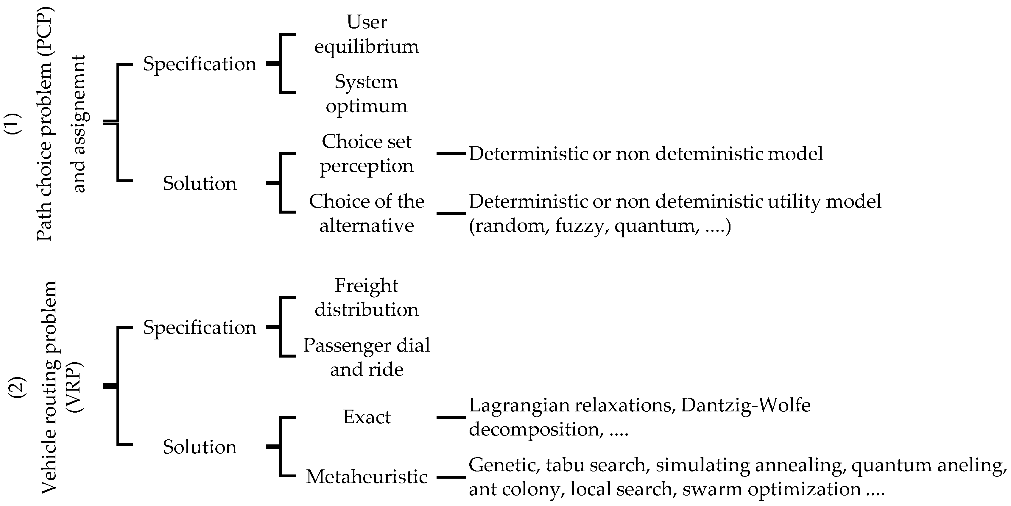
The PCP has the main objective of finding the paths taken by users, given two consecutive pick-up and delivery nodes. In the transport demand assignment to the network, the path choice follows [1] a user equilibrium approach (Wardrop’s first principle [1]) and does not follow an optimal system approach (Wardrop’s second principle [1]). The Wardrop’s first principle provides that each user moves by maximizing his utility function; the system reaches a user equilibrium condition in which no user can improve its utility by a unilateral decision. Wardrop’s second principle considers that users choose cooperatively by maximizing the sum of all users’ utilities; the system reaches the optimum system configuration. In uncongested networks, the two configurations give the same overall utility; in congested networks the optimum configuration of the system generates an overall utility for users greater than or equal to that obtained with the user equilibrium configuration. Wardrop’s first principle is applied at the network level within the assignment problem [1,2,3]. The PCP can be modeled with Mansky’s [4] formulation and two submodels are included: the perception model related to the choice set of alternatives [5] and the choice model related to each alternative [6]. The PCP output is the choice probability or rate for each path of the choice set of alternatives with deterministic or nondeterministic utility models (more details are reported in Section 3).
(2)
The VRP has the main objective of finding the best set of vehicles, routes and paths to follow in the context of transport problems (e.g., freight distribution, dial and ride for passengers, etc.). The problem specified for different transport modes, i.e., cars, buses and trucks [7], freight [8,9], dial and ride [10,11,12], and it is solved with exact or heuristic procedures [13]. Exact solutions can be applied for a small system in acceptable processing time and are based on Lagrangian relaxations or on the Dantzig–Wolfe decomposition. Some papers related to Lagrangian relaxations proposed adopting a branch-and-bound technique [14] or a branch algorithm [15]. Some papers related to the Dantzig–Wolfe decomposition proposed semisoft time windows [16] or rigid time windows [17]. The heuristic solution can be applied for real-size transport systems for the VRP solution in acceptable processing time and in most cases are based on natural metaheuristics procedures. Some papers related to the use of heuristic algorithms proposed adopting a parallel genetic approach [18,19], a tabu search algorithm [20], simulated annealing [21], quantum annealing [22], an ant colony [23], a local search [24], a swarm optimization [25].
Given two consecutive nodes in the route, the PCP cannot be considered: with fixed and predefined static cost; without congestion with specific reference to the urban area; with a deterministic and monocriterion choice (e.g., travel time). A fixed travel cost for a path in an uncongested transport system, sometimes assumed in the VRP, is equivalent to studying the PCP and the VRP separately. This paper tries to bridge the gap between the PCP and the VRP. In this paper, the importance of modelling path choice behavior in the vehicle routing problem is investigated: the routing problem must be modeled considering the path choice with probabilistic models in a congested time-dependent system with pretrip and en route choices.
Considering the objective of the paper, in Section 2, a general approach relating to the transport system analysis and some indications on the specific method proposed in this paper are introduced. Section 3 reports the PCP between two nodes; considering the objective of this paper, in Section 3, a comparison of the path choice models is reported in the consolidated area of the random utility approach. Section 4 reports path choice models in the context of the VRP and some numerical comparisons in a test system. Both Section 3 and Section 4 contain definition and notation, models and discussions subsections. Section 5 reports some conclusions and further developments.
The main contributions of this paper are:
  • The path choice models adopted to simulate a real choice are discussed from the analyst’s point of view (Section 3);
  • The effect of the path choice is considered in the more general VRP (Section 4).

2. Transport System Analysis

The transport system is one of the main components of:
  • SC and communities that is a partnership across the areas of (i.) transport, (ii.) information and communication and (iii.) energy [26];
  • ITS resulting from the integration of knowledge in the areas of (a.) decision support systems (DSS) in transport and (b.) information and communication technologies (ICT).
SC and ITS require transport systems planning that considers the sustainability components (I. economic, II. environmental, III. social), to achieve the 17 goals of the 2030 Agenda for sustainable development of the United Nations.
The VRP is a problem to be solved in a wide area of transport system planning that also requires demand management actions to be implemented in a long, medium, short and real-time time horizon by different interacting actors (Figure 2).

2.1. Actors

Considering a transport system, divided into supply and demand subsystems, three main categories of actors can be identified:
A.
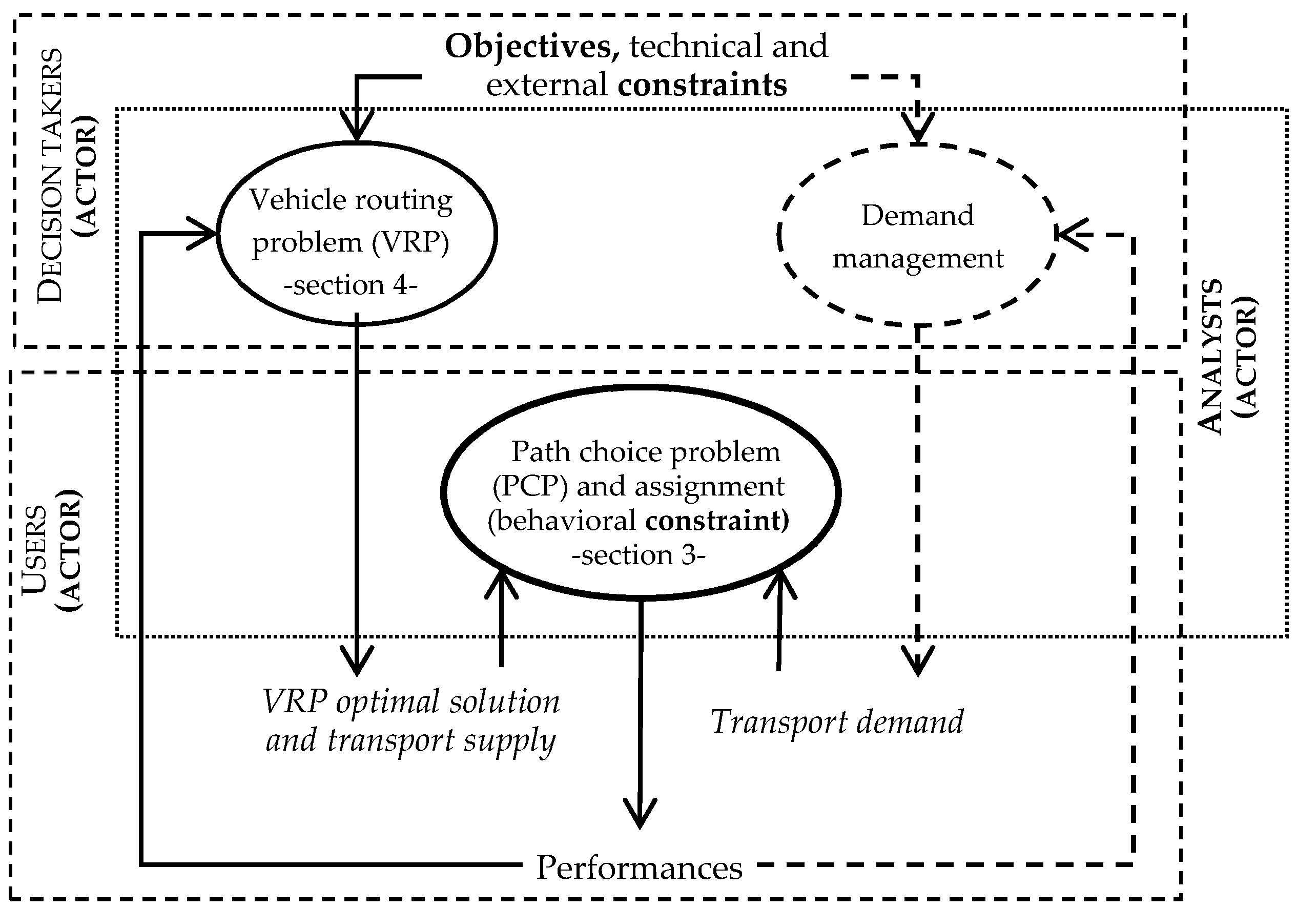
Decision-takers define the objectives to be achieved and define (or must respect) constraints of a technical or regulatory nature; they also take the policy decisions to be implemented for the vehicle routing problem and/or for demand management;
B.
Analysts specify and apply models and procedures for the analysis of the supply–demand interaction (the analysis of network performance with supply models, user behavior with demand models; interactions with supply–demand interaction models), the network design (i.e., a better configuration of the transport network in terms of topology and capacity, vehicle routing reported in this document); demand management (i.e., information on the expected status of the transport system); they also make technical decisions to support decision takers;
C.
Users (citizen) move in the transport system and make pretrip and en route decisions (user behavior) in relation to the supply performance, experience and information received on the system state; users move on the supply designed and the latter is influenced by demand management actions.
In this paper the decision takers and the analysts’ points of view are considered.

2.2. Objectives and Constraints

In a DSS, all components interact with each other, even with circular dependencies. From an operational point of view, the inputs are the objective and the constraints, and the outputs are the actions to be applied on the supply and demand transport subsystems.
(Objectives) The VRP requires the definition of objectives to be achieved in some conflicting cases (some examples could be the minimum cost and time for operators and the maximum pedestrian areas for citizens in urban areas or the maximum revenue for operators and the lowest price for end users). The VRP, considering all the components involved, must be studied with a multicriteria approach considering different types of criteria (even mixed) in different areas:
  • (i.) Transport, (ii.) information and communication and (iii.) energy when considering SC;
  • (a.) DSS and (b.) ICT when considering ITS;
  • (I.) Economic, (II.) environmental and (III.) social criteria when considering sustainability;
  • (A.) Decision-takers, (B.) analysts and (C.) users when considering the involved actors.
(Constraints) Constraints can be classified into external, technical and behavioral. The external constraints represent the quantities that must be respected and imposed for carrying out the activity, i.e., restrictions on circulation in limited traffic areas, regulatory constraints on the characteristics of vehicles that can circulate, time windows allowed for the pick-up and delivery of freight. The technical constraints represent the quantities that must be respected and internal to the problem, i.e., the number and type of vehicles available for the VRP, the contractual characteristics, the quantity of freight that must be picked up and/or delivered to each node. The behavioral constraints represent the choices of the system manager or the driver (pretrip and en route) during the journey between two nodes of the route, and they are conditioned by the state of the transport system. The first two constraints can almost always be linear constraints; the third constraint is always of a nonlinear type.

2.3. Method Proposed

The VRP depends on the PCP, and it cannot be studied by assuming an uncongested network and deterministic path choices. Figure 2 shows the dependency between the VRP and the PCP. The VRP provides the optimal solution, starting from objectives and constraints, and it is a component of the transport supply subsystem. The transport supply subsystem and the transport demand subsystem provide the input for the PCP, which takes place in the context of the assignment of travel demand to the transport networks; this interaction provides the behavioral constraint that must be respected by the VRP. There is a circular dependency between the VRP solution and the constraint provided by the PCP. Transport demand management policies, not included in this paper, also affect the behavioral constraint and it could be included in the context of the overall method.
Decision-takers and analysts are the beneficiary of the proposed method. The decision-takers and companies at the policy level can evaluate the optimal VRP solution with a more accurate methodology for the PCP. The analysist can apply established solution (exact or heuristic) algorithms for the assignment and VRP solutions. The analysts can give more realistic solutions to the decision-makers for their decisions and the solutions can be assumed as an optimal routing strategy.
Behavioral constraints assume a relevance considering the objectives of this paper. The behavioral constraint is modelled with the PCP in the assignment problem, is not linear, and is reported in Section 3. Starting from the path choice specification, in Section 4, the consolidated VRP is also specified considering the effect of the PCP within the VRP with a numerical example.

3. Path Choice Problem and Assignment (Behavioral Constraint)

Two nodes of the pick-up and delivery route are connected by one or more paths. Between two consecutive nodes one or more paths can be perceived and one of these paths is chosen with a behavioral approach. The behavioral constraints are modelled by the analyst taking into account some elements, i.e., the decision of the users and the congestion.

3.1. Definitions and Notations

The definitions and the notations are separated in relation to the path choice and the behavioral constraint.

3.1.1. Path Choice

In a transport system, given a user n (n is not shown below for simplicity) between two nodes u and v of the path, for the user and for the analyst, the following assumptions are considered in this manuscript.
  • Users:
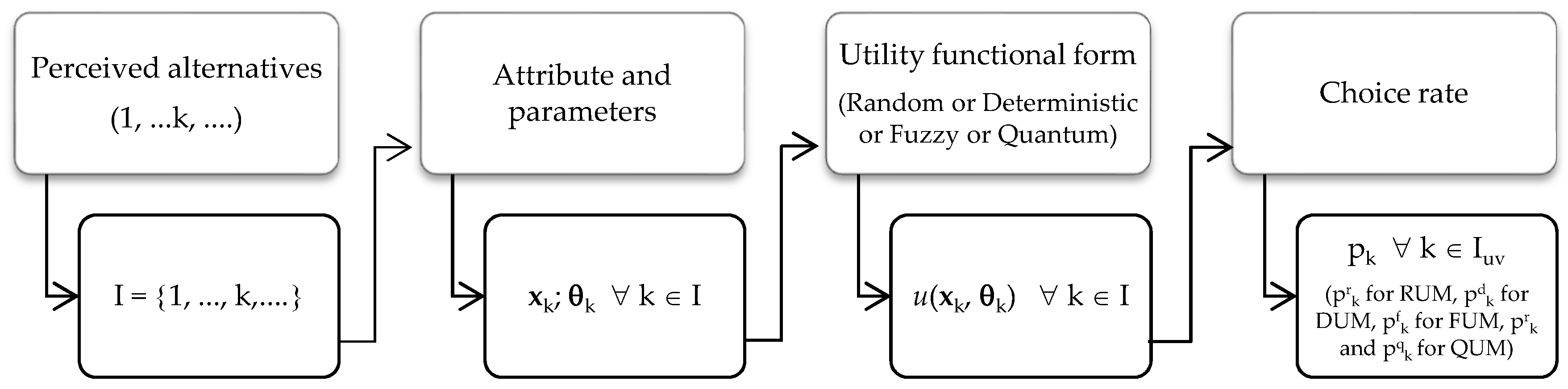
    • Perceive a set (Iuv) of alternatives (k); Iuv = {…, …, k, …} is the set of paths perceived by the decision-maker (system manager or driver) connecting nodes u and v; the entry k of the set Iuv is a perceived path;
    • Associate a perceived utility (uk) to each perceived alternative k; the perceived function (υk) depends on its functional specification, on a vector of known or estimated quantitative attributes of the alternative (xk) and on a vector of unknown parameters (θk) to be calibrated uk = υk(xk, θk);
  • Analysts:
    • Hypothesize that users’ choice among perceived paths is modelled by discrete choice and utility theories, and they evaluate the perceived choice rate vector puv = […, …., pk, …] connecting all pairs of nodes u and v as a function of the perceived utility uk = υk(xk, θk) associated to any path;
    • The perceived choice rate depends on the vector of unknown parameters (θk) to be estimated starting from the data observed with a disaggregated approach (interviews with a sample of users [27], in the state and in the revealed scenarios) or aggregated (traffic flow [27] and web sentiment [28] in the state scenario) by adopting a classic (i.e., maximum likelihood [27]) or Bayesian [28,29] estimator.

3.1.2. Behavioral Constraint

The following variables are defined for the behavioral constraint:
  • f = […, fl, …]’ the traffic flow vector of the links with entry fl, the traffic flow on the link l;
  • c = […, cl, …]’ the cost vector of the links with cl the generalized cost on the link l; it depends on the flow;
  • guv = […, gk, …]’ the generalized path cost vector perceived by the users that connects the pairs of nodes u and v;
  • g = […, guv’, …]’ the vector with all the guv;
  • d = […, duvz, …]’ the demand flow vector; the entry duvz is the demand between origin u, destination v and homogenous class z; note that the demand and the choice rate consider all classes of users, including those who do not belong to the VRP;
  • p = […, puv’, …]’ the rate choice vector (described in Section 3) of the path perceived by the decision-maker (system manager or driver) that connects all the pairs of nodes u and v.

3.2. Models

Models are separated in relation to the path choice and behavioral constraint.

3.2.1. Path Choice

The analyst hypothesizes a functional form for the perceived utility function (υk(xk,θk)). In relation to the hypothesis, the choice rate (pk) of the users who choose each alternative (k) belonging to the set of perceived alternatives is obtained from:
  • A deterministic utility model (DUM), assuming a perceived deterministic utility function; a choice percentage (pdk) is obtained;
  • A random utility model (RUM) assuming a perceived random utility function; a choice probability (prk) is obtained;
  • A fuzzy utility model (FUM) assuming a perceived fuzzy utility function; a fuzzy possibility (pfk) is obtained;
  • A quantum utility model (QUM) assuming a perceived quantum utility function; a random choice probability (prk) and an interference term (pqk) are obtained.
It should be noted that in this paper the path rate was evaluated using discrete choice models and random utility theory. The same considerations can be extended by introducing models that do not belong to the random utility class for evaluating the path rate.
Given a user n and two route nodes, the procedure for evaluating the choice rate is shown in Figure 3.
In the DUM [27], the choice rate (pk) is evaluated with the percentage pdk assigned to the alternatives with the maximum utility value. An alternative has pk = pdk = 1 (or 100%) if it is single with maximum value; the solution is not unique in the case of several alternatives with the maximum perceived utility (any division of 1 between these alternatives is allowed):
pdk ≥ 0 for the alternative of maximum utility with Σk pdk = 1
pk = pdk
In the RUM [27], the perceived utility is modelled as a continuous random utility function. The choice rate (pk) is evaluated with the probability prk that the perceived utility of the alternative is the greatest with respect to all the perceived alternatives:
prk = probability(υk(xk, θ) > υh(xh, θ), ∀ k, h ∈ Irs)
pk = prk
In the FUM [30,31], the perceived utility is modelled as a continuous fuzzy utility number; the possibility qk that the perceived utility of the alternative is greatest is:
pfk = possibility(υk(xk, θk)> υh(xh, θh), ∀ k, h ∈ Irs)
In the QUM (the theory and some applications are reported in [32,33,34]; an aggregate calibration is reported in [35]), the perceived utility is modelled as a quantum utility function with interference between alternatives. The analyst assumes an intermediate decision level with alternatives not clearly perceived by users and not directly observable by the modeler (interference). From the quantum theory, the interference term (pqk) is a function of the probability vector pr with entry prk and the vector α containing the angle in the Hilbert space relative to the interference of each pair of alternatives:
pqk = interference(pr, α)

3.2.2. Behavioral Constraint

The behavioral constraint considers the interaction between supply and demand and starts from supply and demand models. The demand model refers to the dependence of a user’s choice on service transport level indicators and socioeconomic data. The supply model relates to the dependence of the service transport level on the traffic flow.
For simplicity’s sake, before introducing the behavioral constraint, the single dependency is reported considering the dependency between link flow, link cost, path cost, path choice, demand and flow.
  • Link flow–link cost
Considering the small number of VRP vehicles designed in a real problem compared to the total number of vehicles in the transport system, it can be assumed that the output of the VRP (best route) does not affect the state of the transport system in terms of the cost of the link and flow. With this assumption, the VRP cost can be obtained from the flow on the transport system using the link cost function. In a link l, the link cost function gives the link cost from the link flow:
cl = γl(f)     in static a context
cl(t) = γl(f(t))     in dynamic a context
The time-dependent link cost functions is generally assumed as a weighted sum of the cost at the same instant (t) and the cost obtained in a previous interval (t-τ). In this specific case, a dependence on multiple time intervals should be adopted: γl(f(t), f(t-τ)). Considering the scope of this paper, the generic time-dependent function γl() is reported; in this paper, the dynamic assignment is not explored and reference is made to the specific literature for further information [36]. The static cost can be assumed as a particular case of the dynamic cost considering that it is assumed to depend on the flow, but it is constant over time. From the link cost functions, the vector of link cost functions are obtained:
c(t) = γ(f(t)) = […,γl(f(t)), …]’
  • Link cost–path cost
The path cost g is obtained as the sum of the additive (with respect to the link) path cost (gA with entry gkA) and the nonadditive path cost (gNA with entry gkNA):
gk(t) = gkA(t) + gkNA = Σl∈k γl(f(t)) + gkNA
Considering the whole path k between all nodes u and v, the path choice vector is defined as (g), dependent on the link flow vector:
g(t) = ξ(f(t))
  • Path cost–path choice
 
In the DUM, it is assumed that each user, for each alternative k, from u to v, perceives a deterministic utility given by the linear combination (vk = θk’ xk) of the attributes (xk) with respect to the parameter (θk). Users choose the alternative of greatest perceived utility. In nondeterministic models it is assumed that each user:
  • Perceives a nondeterministic utility (uk) with expected (or barycenter) value (vk=E(uk)) given by the linear combination of the attributes with respect to the parameter (vk = θk’ xk);
  • Chooses the alternative of maximum perceived utility, and the analyst can evaluate the choice rate (pk) for each alternative (k) belonging to the perceived choice set (Irs).
Note that the quantitative attributes of the alternative k include all the variables that influence the path choice. In vector xk, one element (it could also be the only one) is the cost gk of the path k. Considering all the alternative, the choice rate vector p depends on the path cost vector (g), and the path cost depends on the link flow vector (f). For this reason, the choice rate (pk) is a function of the flow vector f:
pk(t) = υuv(f(t))
Given the nodes u and v connected by the path k, the PCP defines a perceived set Iuv of alternatives and for each alternative belonging to Iuv, a choice rate pk is evaluated. Considering all the perceived path k between all nodes u and v, the rate choice vector (p = [….,puv’, …]’) is defined, depending on the link flow vector:
p(t) = υ(f(t))
More details on the PCP are given in Section 3.2.1.
  • Path cost–demand
The demand duvz is the flow of passenger and freight between u and v for the homogeneous class z. The demand model depends on the users’ choice (purpose and time of departure and/or arrival, origin and destination, mode and route). The vehicles considered in the VRP are included in the demand. The demand is also evaluated with the discrete choice and utility theory described for the PCP. The travel demand d, like p, also depends on a set of attributes, including the path cost g.
  • Demand–flow
The flow on each link l is given by the weighed sum (with weight βn) of the demand flow through the link, considering all the origins u, all the destinations v and all classes z of users:
fl(t) = Σz Σu Σv Σk_containing_l βz • pk(t) • duvz
Note that in pk, the user class must be considered, but it is omitted here for simplicity.
Behavioral constraints can be described by the circular dependency between link flows (f), link costs (c), path cost (g), path choice (p) and demand (d) that generate the flows (f).
In a dynamic context, within-day and/or day-to-day dynamic approaches can be adopted [27,36], and the flow vector has a time dependency:
f(t) = ζ(f(t))
where ζ() is the function that describes the dynamic dependency on time.
Note that, as already reported for the costs, in the dynamic models, the flow is often considered as the weighted sum of the flow obtained at the same instant t, and the flow obtained in a previous interval t-τ. In this specific case, a function further specified below should be adopted: ζ(f(t), f(t-τ), t, t-τ).
In the static context, the solution derives from a fixed-point model [27] and ξ() is the loading flow function.

3.3. Discussion

In the DUM, the deterministic perceived utility function can be viewed mathematically as a random perceived utility function with zero limiting variance. The sum of all the percentages on all the alternatives is equal to one. The assumption of a deterministic choice of the path is not possible for several reasons: the analyst does not know exactly the behavior of the system manager and the drivers; the analyst cannot accurately predict the state of the transport system; and the state of the transport system is congested and is time-dependent.
In the RUM, different distributions can be adopted for the continuous random utility function (i.e., Gumbel for the Logit class; Weibull for the Weibit class; multivariate Gauss for the Probit class; multivariate gamma for the Gammit class [37]; more than one random utility functions for the mixed class). Considering all the alternatives, the random utility function can be: identical (homoscedastic) or nonidentical (heteroscedastic) between users, alternative or time; independent or joint distributions; with deterministic θ parameters or with parameters distributed with a random function; in this case, the utility has two random effects, one relating to the entire utility and one for each random parameter; for more details see [38]. The sum of all probabilities on all alternatives is equal to one.
In the FUM, the sum of all possibilities over all alternatives can be greater than one. For this reason, the choice rate (pk) is evaluated by the possibility qk with a transformation function; one of these functions was proposed by Klir [39] to be:
pk = (pfk)γh∈I (pfh)γ
with γ a parameter greater than zero to be calibrated.
In the QUM, the interference term decreases or increases the probability evaluated with a random utility function in relation to the level of interference (unclear perception) between the alternatives. It can be demonstrated that the interference term pqk assumes values in relation to the level of interference and guarantees that the sum of all rate probability on all alternatives is one (pqk ∈ [–prk; 1−prk] and Σk pqk = 0) and the rate (pk) is evaluated with:
pk = prk + pqk
For the FUM and the QUM, in relation to the specification of the utility function, the same model described in the case of the random perceived utility can be obtained (identical or not identical distribution; homoscedastic or heteroscedastic; not jointly or jointly; deterministic or random parameters).
Note that the FUM and the QUM cannot be considered as a particular or a general case of the RUM: they are different from the RUM. The main reasons are as follows: they consider a different user’s behavior not representable by the analyst with random utility models; the fuzzy model does not evaluate a probability, it evaluates a possibility, and the sum on all the alternatives is not equal to one; the quantum model evaluates the interference deriving from considering the interference between the alternatives unobservable by the analyst and by the users; the quantum model modifies with an additive term the random probability.
A summary of the reported path choice models with a comparison of the main characteristics is reported in Table 1.

4. Vehicle Routing Problem

In the VRP, the user, the driver and/or the system manager decide which path to follow. The decision can be supported by a DSS. As reported in Section 3, the deterministic path choice assumption is not close to reality, and the effect of the route choice must be considered in the VRP.

4.1. Definitions and Notations

The VRP provides the best routes (Ω) to follow in the context of transport problems (i.e., freight distribution, dial and ride for passengers, etc.). The route to follow is constrained by external and technical constraints and behavioral constraints relating to the path (k) chosen between two consecutive nodes (r, s) of the route.
The following variables are defined in the VRP:
  • r and s are two pick-up and delivery points to be served by the VRP;
  • Ω = [[… ωv,rs…]] is the matrix of routes defined in term of sequences of nodes to be visited by a set of vehicles; the entry ωv,rs of the matrix Ω is equal to one if the vehicle v connects the nodes r and s, and it is zero otherwise;
  • g(VRP) = […, g(VRP)rs’, …]’ with g(VRP)rs = […, g(VRP)k, …]’ the generalized path cost vector perceived by the decision-maker (system manager or driver) connecting the pairs of nodes r and s to be visited for pick-up and delivery;
  • g(VRP)(t) = ξ(f(t)) with ξ() the vector of path cost functions defined in the Section 3;
  • p(VRP) = […, p(VRP)rs’, …]’ with p(VRP)rs = […, p(VRP)k, …]’ the vector of path rate connecting the pairs of nodes r and s to be visited for pick-up and delivery;
  • p(VRP)(t) = υ(f(t)) with υ(f(t)) the vector of path rate functions defined in Section 3;
  • z(f, Ω, g(VRP), p(VRP), t) = […, zb(f, Ω, g(VRP), p(VRP)), …]’ is the multicriteria objective function with entry zb() relative to the generic criteria adopted in the multicriteria optimization;
  • STE is the set of feasible technical and external constraints;
  • Sf is the set of admissible flow (i.e., non-negative, congruent with the passenger and freight demand on the routes, paths and nodes).

4.2. Models

In order to better highlight the variables that influence the VRP considering the objectives of this work, in the optimization specification reported in this section, the main variables and constraints strongly dependent on the path choice are explicitly reported (more details for the path choice are reported in Section 3). The other variables and constraints are reported with a compact specification; this is particularly evident for the set of technical and admissible constraints which require many equations, and they are important in the problem; they are considered but are not specified.
In the real problem, the number of vehicles of VRP is small compared to the total number of vehicles in the transport system. Under these conditions, it can be assumed that the equilibrium or dynamic state of the transport system is little influenced by the path and route choice of the vehicles belonging to the VRP. Therefore, it can be hypothesized that the path cost, the rate choice and the related path costs of the VRP vehicles can be evaluated by considering the flow deriving from the behavioral constraint (respectively, g(VRP) = ξ(f(t)) and p(VRP) = υ(f(t))). With this hypothesis, the VRP can be defined in the following optimization form:
minf, Ω   z(f, Ω, g(VRP)(t), p(VRP)(t), t)                          
subject to                                                                             
f(t) = ζ(f(t), f(t-τ), t-τ)   →   //behavioral constraint     
ΩSTE     →       //external and technical constraints
g(VRP)(t) = ξ(f(t))    →    //path cost evaluation for VRP
p(VRP)(t) = υ(f(t))    →    //path rate evaluation for VRP

4.3. Discussion

The first consideration concerns the multicriteria objective function. As reported in Section 2, different actors interact with each other (decision-takers, analysts, users) and objectives of different classes can be considered (e.g., transport, information and communication, energy considering the smart city; economic, environmental, social criteria considering sustainability). The objectives can also be conflicting with each other (e.g., a high speed and short travel time could conflict with the pedestrian area for citizens). For this reason, it is necessary to adopt a multicriteria optimization.
In the real case, it can be observed that the drivers do not follow the best route and do not consider the same cost estimation criterion. The results are also confirmed in [40].
The paper [40] analyzed 12 routes with more than four visited nodes in each route. In the 12 routes, 73 paths were chosen. Three criteria were adopted for the VRP and the PCP for route optimization and path generation: minimum time, minimum distance and minimum energy consumption. The paper [40] showed that there was not a single criterion adopted in the choice of routes and paths. Minimum times were frequently adopted in the VRP (about 70% of similarity); the three criteria were used in the PCP (approximately 75% of similarity). It confirmed the necessity to use a multicriteria approach in the objective function for the VRP and the need to evaluate the rate choice. The importance of path planning was also simulated in [41].
The second consideration relates to the evaluation of the path rate. Given a pick-up and delivery pair of nodes r and s (the time dependence is omitted for simplicity’s sake):
  • In the DUM, for each pair of pick-up and delivery nodes, the generalized minimum cost is:
g(VRP)minrs = minrs g(VRP)k       ∀ g(VRP)kg(VRP)rs
  • In the RUM, the FUM and the QUM, which best represent reality, a rate choice is evaluated for each perceived path and some indicators must be evaluated (i.e., the expected perceived cost for all paths or for the path with a rate choice higher than a threshold or a path that satisfies a decision criterion); if the expected cost values for all the perceived paths are considered, the generalized cost is:
g(VRP)Ers = ΣkIrs    p(VRP)k • g(VRP)k       ∀ k ∈ Irs
Note g(VRP)Ers is obtained with a convex combination of path cost g(VRP)k ≥ g(VRP)minrs and g(VRP)Ers ≥ g(VRP)minrs. It means that the VRP solved with the minimum cost for each pair of nodes is a lower bound of the real perceived cost and for this reason, the VRP solution cannot be obtained with the DUM. The DUM cannot guarantee that the best solution is the same as that obtained with the RUM, the FUM or the QUM.
These considerations were verified in a numerical application. A small network size was considered (Figure 4) to allow the reader to follow all the steps of the procedure. In the test network, one depot (number 1) and four pick-up and delivery nodes (2, 3, 4, 5) were considered. The pick-up and delivery times at each node were fixed and were not reported into the routing time because it did not affect the best sequence of nodes to visit.
The path cost was obtained with a fixed-point model in a static approach assuming a congested network or with a day-to-day and/or within-day model in a dynamic approach assuming a time-dependent network. From the state of the transport system, it was assumed that the cost in the shortest path (first, G(1)), which connects the pair of nodes in the routing problem, was equal to:
Nodes12345
1--8.22.21.46.4
29.1--9.09.56.7
G(1) =32.59.9--3.08.5
41.610.03.3--6.7
57.07.49.37.4--
It was assumed that three paths were perceived in each pair of nodes (a different number of paths perceived in each pair of nodes could also be assumed). For the pair of nodes 1–4, it was assumed that the cost in the second path was equal to the minimum cost increased by 50% and the cost in the third path was equal to the minimum cost increased by 100%. In the other pairs of nodes, it was assumed that the cost in the second path was equal to the minimum cost increased by 10% and the cost in the third path was equal to the minimum cost increased by 20%.
The costs in the second (G(2)) and in the third path (G(3)) were:
Nodes12345 Nodes12345
1--9.12.52.17.0 1--9.92.72.87.7
210.0--9.910.07.4 211.0--11.011.08.0
G(2) =32.711,0--3.39.3G(3) =33.012.0--3.610.0
41.711,03.6--7.4 41.913.04.0--8.0
57.78.110.08.1-- 58.58.911.08.9--
The cost vector gVRP specified in the paper was obtained starting from the three matrices: the pairs of nodes were reported in sequence and the three paths cost were reported for each pair:
g(VRP) = [8.2; 9.1; 9.9; 2.2; 2.5; 2.7; …; 9.3; 10.0; 11.0; 7.4; 8.1; 8.9]’
Considering the DUM for the PCP, the minimum cost for each pair of nodes was considered. The best route was with the sequence of nodes 1-4-5-2-3-1 with an expected travel cost for the route of 27.0, which was the sum of the cost in the minimum paths.
Considering the RUM for the PCP, with Logit choice with a Gumbel parameter of 2.5 [6,27], given a pair of nodes, the rate choice for path k was:
p(VRP)k = e−gk/θh e−gh/θ
The path rate vector p(VRP) was:
p(VRP) = [45%; 32%; 23%; 37%; 33%; 30%; …; 46%; 32%; 22%; 44%; 32%; 24%]’
With the RUM for the PCP, the best route was with the sequence of nodes 1-5-2-3-4-1 with 29.6 as the estimated travel cost for the route given by the weighted sum (with probability) of the cost considering three routes in each pair of nodes.
In this particular case, the optimal routing considering the DUM and the RUM for the PCP gave different results in terms of node sequences. The expected cost evaluated with the RUM was greater than the expected cost evaluated with the DUM. This case demonstrates that applying the DUM to solve the VRP can give a different solution than the case without the DUM. Considering the DUM is not a real case, it should be avoided in the VRP.

5. Conclusions

In this paper, the influence of the PCP in the VRP was investigated. Initially, the transport system analysis and the main actors involved were described, as well as the objectives considering different classifications and constraints. From this analysis emerged the need to study the problem through a multicriteria approach that considered the choice of the path within a behavioral constraint.
The behavioral nonlinear constraint can be represented by studying the state of equilibrium and the dynamic evolution of the transport system using path choice models. For path choice models, deterministic models cannot be used considering that a future state of the transport system is influenced by various factors such as congestion, incomplete information of the system, etc.
The main discrete choice models of random utility were reported together with the specifications for calculating the path rate. The expected value of the perceived cost between each pair of nodes was calculated and inserted into the general optimal model of the VRP. In real problems, the number of vehicles considered in the VRP is lower compared to the total number of vehicles in circulation. Therefore, it is possible to assume that the path choice probability of the vehicles of the VRP does not affect the state of the transport system.
The model was applied to a test network with assumptions on the cost values and choice rate. It was seen that, in the adopted test network, the best route changed by establishing a deterministic or nondeterministic path choice model.
The results obtained provide policy recommendations for analysts regarding the path choice models to be adopted for the VRP solution. Using costs for a single path could provide different VRP solutions than using all perceived paths. However, considering that the VRP refers to a future state of the system, it is not possible to solve it through deterministic and hypothetical costs, even if historical. The solution of the PCP within the VRP is recommended. Decision-makers also benefit from this model specification because it better represents user behavior.
In term of applicability, the model has limits regarding the optimization as the nonlinear behavioral constraint requires adequate procedures to find a solution in acceptable processing times. In the proposed methodology, the consolidated algorithms used for the solution of the assignment models, including the solution of the PCP, and for the solution of the VRP can be adopted. In practice, in real-size problems and for real-time solutions, it requires suitable activities for the integration of the two algorithms. The model presented requires the development of optimal procedures for the solution of real-scale problems in the future. It could start from excellent metaheuristic procedures adopted for the solution of the VRP, integrating them with the consolidated procedures that solve the behavioral constraint.

Funding

This research is partially supported by DIIES—Università di Reggio Calabria and by the project “La Mobilità per i passeggeri come Servizio–MyPasS”, Fondi PON R&I 2014–2020 e FSC, Progetti di Ricerca PNR 2015–2020, codice identificativo ARS01_01100.

Institutional Review Board Statement

Not applicable.

Informed Consent Statement

Not applicable.

Data Availability Statement

Not applicable.

Acknowledgments

The author thanks the anonymous reviewers for their useful comments and interesting suggestions.

Conflicts of Interest

The author declares no conflict of interest.

Abbreviations

DSS, decision support system; DUM, deterministic utility model; ICT, intelligent and communication technology; FUM, fuzzy utility model; PCP, path choice problem; QUM, quantum utility model; RUM, random utility model; SC, smart city; VRP, vehicle routing problem.

References

  1. Wardrop, J.G. Some Theoretical Aspects of Road Traffic Research. Proc. Inst. Civ. Eng. 1952, 1, 325–362. [Google Scholar] [CrossRef]
  2. Dial, R.B. A probabilistic multipath traffic assignment algorithm which obviates path enumeration. Transp. Res. 1971, 5, 83–111. [Google Scholar] [CrossRef]
  3. Daganzo, C.F.; Sheffi, Y. On Stochastic Models of Traffic Assignment. Transp. Sci. 1977, 11, 253–274. [Google Scholar] [CrossRef] [Green Version]
  4. Manski, C.F. The structure of random utility models. Theory Decis. 1977, 8, 229–254. [Google Scholar] [CrossRef]
  5. Ben-Akiva, M.; Bergman, M.J.; Daly, A.J.; Ramaswamy, R. Modelling inter urban route choice behaviour. In Proceedings of the Ninth International Symposium on Transportation and Traffic Theory, Delft, The Netherlands, 11–13 July 1984; Volmuller, J., Hamerslag, R., Eds.; CRC Press: Boca Raton, FL, USA, 1984; pp. 299–330. [Google Scholar]
  6. Ben-Akiva, M.E.; Lerman, S.R. Discrete Choice Analysis. Theory and Application to Travel Demand. MIT Press Series in Transportation Studies; Manheim, M., Ed.; MIT Press Ltd.: Cambridge, MA, USA, 2018. [Google Scholar]
  7. Dantzig, G.B.; Ramser, J.H. The Truck Dispatching Problem. Manag. Sci. 1959, 6, 80–91. [Google Scholar] [CrossRef]
  8. Vidal, T.; Laporte, G.; Matl, P. A concise guide to existing and emerging vehicle routing problem variants. Eur. J. Oper. Res. 2020, 286, 401–416. [Google Scholar] [CrossRef] [Green Version]
  9. Napoli, G.; Micari, S.; Dispenza, G.; Andaloro, L.; Antonucci, V.; Polimeni, A. Freight distribution with electric vehicles: A case study in Sicily. RES, infrastructures and vehicle routing. Transp. Eng. 2021, 3, 100047. [Google Scholar] [CrossRef]
  10. Cordeau, J.-F. A Branch-and-Cut Algorithm for the Dial-a-Ride Problem. Oper. Res. 2006, 54, 573–586. [Google Scholar] [CrossRef] [Green Version]
  11. Chen, L.-W.; Hu, T.-Y.; Wu, Y.-W. A bi-objective model for eco-efficient dial-a-ride problems. Asia Pac. Manag. Rev. 2022, 27, 163–172. [Google Scholar] [CrossRef]
  12. Chu, J.C.-Y.; Chen, A.Y.; Shih, H.-H. Stochastic programming model for integrating bus network design and dial-a-ride scheduling. Transp. Lett. 2020, 14, 245–257. [Google Scholar] [CrossRef]
  13. Laporte, G. What you should know about the vehicle routing problem. Nav. Res. Logist. 2007, 54, 811–819. [Google Scholar] [CrossRef]
  14. Fisher, M.L. Optimal Solution of Vehicle Routing Problems Using Minimum K-Trees. Oper. Res. 1994, 42, 626–642. [Google Scholar] [CrossRef]
  15. Kallehauge, B.; Larsen, J.; Madsen, O.B. Lagrangian duality applied to the vehicle routing problem with time windows. Comput. Oper. Res. 2006, 33, 1464–1487. [Google Scholar] [CrossRef]
  16. Qureshi, A.; Taniguchi, E.; Yamada, T. An exact solution approach for vehicle routing and scheduling problems with soft time windows. Transp. Res. Part E Logist. Transp. Rev. 2009, 45, 960–977. [Google Scholar] [CrossRef]
  17. Azi, N.; Gendreau, M.; Potvin, J.-Y. An exact algorithm for a single-vehicle routing problem with time windows and multiple routes. Eur. J. Oper. Res. 2007, 178, 755–766. [Google Scholar] [CrossRef]
  18. Allahviranloo, M.; Chow, J.Y.; Recker, W.W. Selective vehicle routing problems under uncertainty without recourse. Transp. Res. Part E Logist. Transp. Rev. 2014, 62, 68–88. [Google Scholar] [CrossRef]
  19. Abbasi, M.; Rafiee, M.; Khosravi, M.R.; Jolfaei, A.; Menon, V.G.; Koushyar, J.M. An efficient parallel genetic algorithm solution for vehicle routing problem in cloud implementation of the intelligent transportation systems. J. Cloud Comput. 2020, 9, 1–14. [Google Scholar] [CrossRef]
  20. Gribkovskaia, I.; Laporte, G.; Shyshou, A. The single vehicle routing problem with deliveries and selective pickups. Comput. Oper. Res. 2008, 35, 2908–2924. [Google Scholar] [CrossRef]
  21. Tavakkoli-Moghaddam, R.; Safaei, N.; Gholipour, Y. A hybrid simulated annealing for capacitated vehicle routing problems with the independent route length. Appl. Math. Comput. 2006, 176, 445–454. [Google Scholar] [CrossRef]
  22. Syrichas, A.; Crispin, A. Large-scale vehicle routing problems: Quantum Annealing, tunings and results. Comput. Oper. Res. 2017, 87, 52–62. [Google Scholar] [CrossRef]
  23. Dorigo, M.; Stützle, T. Ant Colony Optimization; MIT Press: Cambridge, MA, USA, 2004. [Google Scholar]
  24. Rivera, J.C.; Afsar, H.M.; Prins, C. A multistart iterated local search for the multitrip cumulative capacitated vehicle routing problem. Comput. Optim. Appl. 2014, 61, 159–187. [Google Scholar] [CrossRef]
  25. Marinaki, M.; Marinakis, Y. A Glowworm Swarm Optimization algorithm for the Vehicle Routing Problem with Stochastic Demands. Expert Syst. Appl. 2016, 46, 145–163. [Google Scholar] [CrossRef]
  26. European Commission, Smart cities and communities—European innovation partnership, Communication from the Commission, C(2012) 4701, 2012. Available online: https://digital-strategy.ec.europa.eu/en/library/smart-cities-and-communities-european-innovation-partnership-communication-commission-c2012-4701 (accessed on 3 January 2023).
  27. Cascetta, E. Transportation Systems Engineering: Theory and Methods; Springer: Berlin/Heidelberg, Germany, 2009. [Google Scholar]
  28. Vitetta, A. Sentiment Analysis Models with Bayesian Approach: A Bike Preference Application in Metropolitan Cities. J. Adv. Transp. 2022, 2022, 2499282. [Google Scholar] [CrossRef]
  29. Washington, S.; Congdon, P.; Karlaftis, M.G.; Mannering, F.L. Bayesian Multinomial Logit: Theory and Route Choice Example. Transportation Research Record. J. Transp. Res. Board 2009, 2136, 28–36. [Google Scholar] [CrossRef]
  30. Henn, V. Path choice making under uncertainty: A fuzzy logic based approach. In Fuzzy Sets-Based Heuristics for Optimization; Verdegay, J., Ed.; Springer: New York, NY, USA, 2003; pp. 277–292. [Google Scholar]
  31. Henn, V.; Ottomanelli, M. Handling uncertainty in route choice models: From probabilistic to possibilistic approaches. Eur. J. Oper. Res. 2006, 175, 1526–1538. [Google Scholar] [CrossRef]
  32. Busemeyer, J.R.; Wang, Z.; Townsend, J.T. Quantum dynamics of human decision-making. J. Math. Psychol. 2006, 50, 220–241. [Google Scholar] [CrossRef]
  33. Lipovetsky, S. Quantum paradigm of probability amplitude and complex utility in entangled discrete choice modeling. J. Choice Model. 2018, 27, 62–73. [Google Scholar] [CrossRef]
  34. Vitetta, A. A quantum utility model for route choice in transport systems. Travel Behav. Soc. 2016, 3, 29–37. [Google Scholar] [CrossRef]
  35. Di Gangi, M.; Vitetta, A. Quantum utility and random utility model for path choice modelling: Specification and aggregate calibration from traffic counts. J. Choice Model. 2021, 40, 100290. [Google Scholar] [CrossRef]
  36. Cantarella, G.E.; Watling, D.P.; de Luca, S.; Di Pace, R. Dynamics and Stochasticity in Transportation Systems; Tools for Transportation Network Modelling; Elsevier: Amsterdam, The Netherlands, 2020. [Google Scholar] [CrossRef]
  37. Cantarella, G.E.; Binetti, M.G. Stochastic Assignment with Gammit Path Choice Models. In Transportation Planning; Patriksson, M., Labbé, M., Eds.; Applied Optimization; Springer: Boston, MA, USA, 2002; Volume 64. [Google Scholar]
  38. de Luca, S. Discrete choice modelling with application to route and departure time choice. In Dynamics and Stochasticity in Transportation Systems; Tools for Transportation Network Modelling; Cantarella, G.E., Watling, D.P., de Luca, S., Di Pace, R., Eds.; Appendix A; Elsevier: Amsterdam, The Netherlands, 2020; pp. 195–263. [Google Scholar]
  39. Klir, G.J. A principle of uncertainty and information invariance*. Int. J. Gen. Syst. 1990, 17, 249–275. [Google Scholar] [CrossRef]
  40. Croce, A.I.; Musolino, G.; Rindone, C.; Vitetta, A. Route and Path Choices of Freight Vehicles: A Case Study with Floating Car Data. Sustainability 2020, 12, 8557. [Google Scholar] [CrossRef]
  41. Kong, S.; Zhong, Z.; Zhang, J. Bi-objective vehicle routing problems with path choice and variable speed. Complex Syst. Complex. Sci. 2022, 19, 74–80. [Google Scholar]
Figure 1. State of the art’s classification.
Algorithms 16 00047 g001
Figure 2. Functional architecture in a decision support system.
Algorithms 16 00047 g002
Figure 3. Path choice model: variables and parameters.
Algorithms 16 00047 g003
Figure 4. Test network.
Algorithms 16 00047 g004
Table 1. Comparison between the characteristics of the utility models.
Utility Model
(UM)
NamePerceived Utility
Function υk(xk, θk)
DUM, RUM, FUM, QUM
Evaluation
Choice Rate
pk
Starting from Random Utility
Deterministic
(DUM)
pdkDeterministic
utility function
pdk ≥ 0 for the alternative
of maximum utility
with Σk pdk = 100%
pk = pdkLimit with zero variance
Random
(RUM)
prkContinuous
random utility
function
prk = pr(υk(xk, θk) > υh(xh, θh), ∀ k,h∈I)
(pr means probability)
pk = prkSame
Fuzzy
(FUM)
pfkContinuous
fuzzy utility
number
pfk = po(υk(xk, θk) > υh(xh, θh), ∀ k,h∈I)
(po means possibility)
pk = (pfk)γh∈I(pfh)γNonlinear
transformation
(possibility
vs. probability)
Quantum
(QUM)
pqkQuantum
Utility function
with interference
pqk = interference(pr, α)
(it respects pqk ∈ [–prk; 1−prk]
and Σk pqk = 0%)
pk = prk + pqkAdditive term
(quantum
vs. probability)
Disclaimer/Publisher’s Note: The statements, opinions and data contained in all publications are solely those of the individual author(s) and contributor(s) and not of MDPI and/or the editor(s). MDPI and/or the editor(s) disclaim responsibility for any injury to people or property resulting from any ideas, methods, instructions or products referred to in the content.

