

Finding Bottlenecks in Message Passing Interface Programs by Scalable Critical Path Analysis

 , , , , , ,
Abstract
:1. Introduction
2. Related Work
- The critical path cannot contain program edges leading to receive nodes that incur a blocking wait time.
- The critical path cannot contain communication edges, which do not lead to blocking wait times.
3. Approach Overview
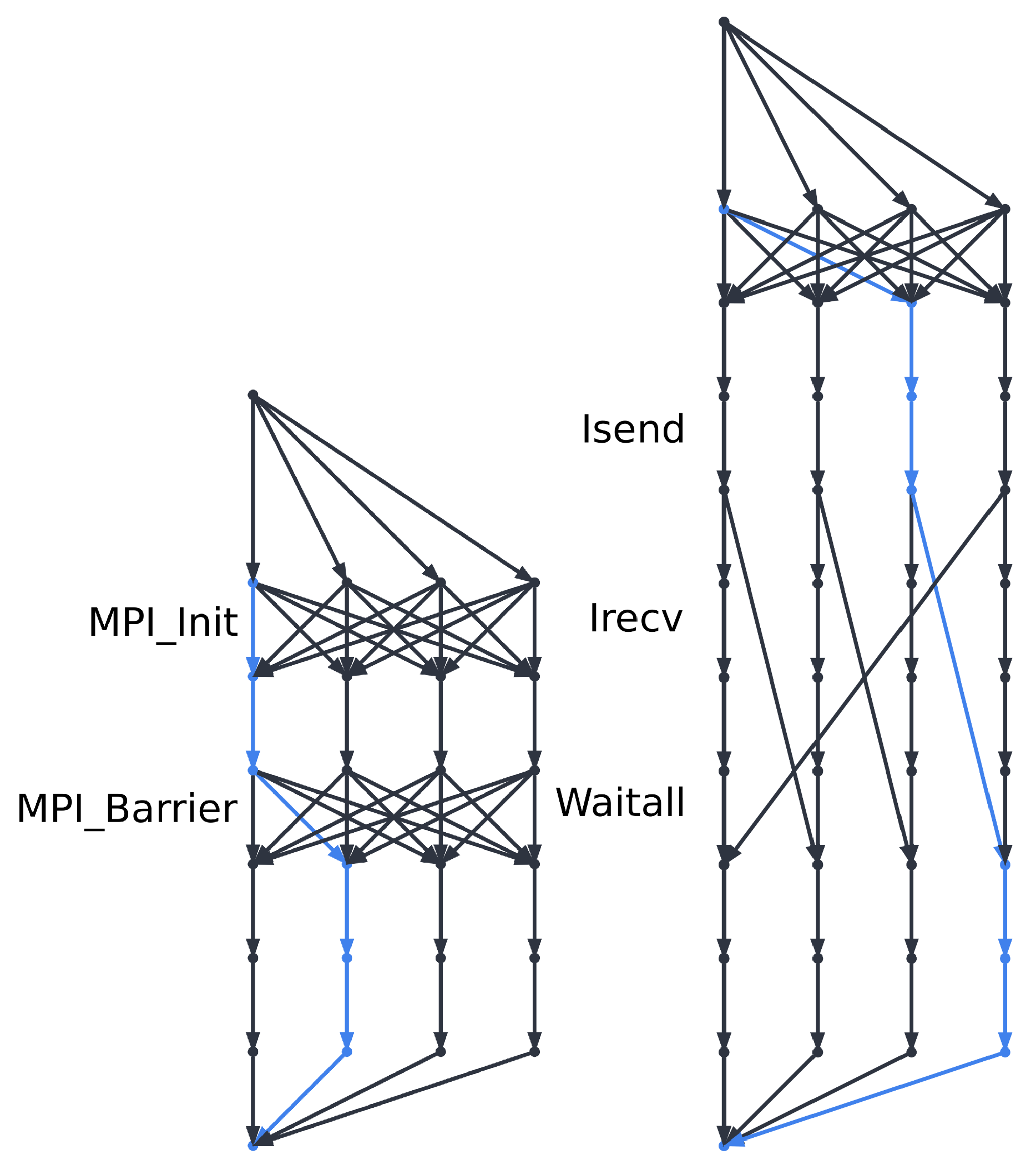
- Synchronize timestamps of all MPI processes.
- We use a monotonic clock to save timestamps and synchronize clocks using MPI_Allreduce at the start of the program (in MPI_init).
- Log relevant MPI operations with relevant arguments and start–end timestamps. Link local operations into a linear graph.
- We log every MPI call that involves process communication (e.g., MPI_Send, MPI_Recv, MPI_Reduce, MPI_Broadcast, etc.) using the MPI profiling interface.
- For each MPI call, we log the start timestamp, end timestamp, function name, and function arguments (except user data).
- Each MPI process maintains its own log-in memory.
- The log represents a linear graph: an edge connects the log record N to the log record . The weight of the edge equals the difference between the start time and the end time N.
- After MPI_Finalize, link corresponding local and remote operations (send/recv) to produce the final graph.
- After the previous step, we have the log which is distributed across all MPI processes, and we now convert it to the graph. The local log contains only the edges for the vertices of the corresponding MPI process, and we need to create edges between the different MPI processes. (For each MPI call, we have a starting and ending vertex that is connected with the edge.)
- To achieve this, each MPI process goes over all log records, and, for each MPI call, it requests information from the processes that were involved in this call. (It does not matter whether the receiver or sender obtains the information; we need to create the edges only in one MPI process not to produce duplicates.) The information is requested using the appropriate MPI calls (MPI_Send, MPI_Recv, MPI_Reduce, etc.), and the calls are different for each collective and point-to-point operation.
- We can optimize the graph during conversion using techniques from [2]. For example, for MPI_Barrier, we need only one edge that connects the starting vertex for the last process to reach the barrier with the ending vertex for the last process to leave the barrier. For other blocking collective operations, the optimizations are similar.
- Find the critical path using different algorithms and existing data distribution between nodes.
- Now, we have the final graph that is composed of local graphs, which are stored in the corresponding MPI processes. The global graph is partitioned already, and all we need is to find the critical path.
- For parallel processing, we need to map each vertex and edge of the graph to the rank of the MPI process that stores this edge or vertex. This is trivial to implement in the previous step by saving the rank of the target MPI process for each inter-process edge; all other vertices and edges are local to the node.
- There are several algorithms for parallel graph search. The most common one is Delta-stepping (see Section 4). We make all weights negative and start the search from the vertex with the largest timestamp (which can also be determined in the previous step).
4. Methods and Algorithms for Finding Critical Path
4.1. Sequential Dijkstra
4.2. Sequential Delta-Stepping
4.3. Parallel Dijkstra
- We start with the nodes and edges distributed across the MPI processes: each process stores only the nodes that correspond to the MPI calls that were made by this process and all incoming edges of these nodes. The process that contains a particular node is determined using its global identifier and simple division.
- Each process pushes the source node to its own per-process queue and the main loop begins.
- For each iteration, each process extracts the next node from the queue and finds all incoming edges of this node. Then, we group the edges by the rank of the process that stores the source node of each edge. After that, each process sends each non-empty group to the corresponding rank.
- After the communication, each process concatenates all of the groups of edges that were received from other processes. The resulting edges are scanned, and, if the new distance is smaller, then the distance is updated, and the source node of the edge is pushed into the queue with the new distance (distances are stored in the local hash table).
- The iterations continue until all per-process queues are empty. If the queue becomes empty, then the corresponding process takes part in the collective operations but does not process nodes from the queue.
- After the last iteration, the hash table that stores the path that was followed by the algorithm is gathered in the first MPI process. Then, the algorithm terminates.
4.4. Parallel Splits
- If some asynchronous MPI operations have not been completed yet, then this is not a synchronization point.
- If any edges of the collective MPI operation have a negative time, then this is not a synchronization point.
- Otherwise, it is a global synchronization point, and we can split the graph at this point.
- Run a sequential algorithm on each split sequentially.
- Run a parallel algorithm on each split sequentially.
- Run a parallel algorithm on each split in parallel.
- Run a sequential algorithm on each split in parallel.
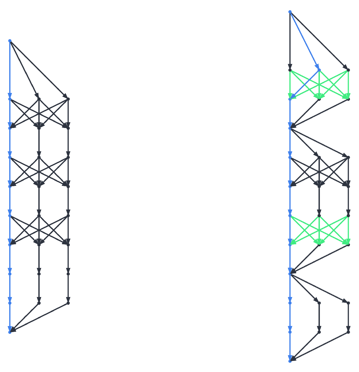
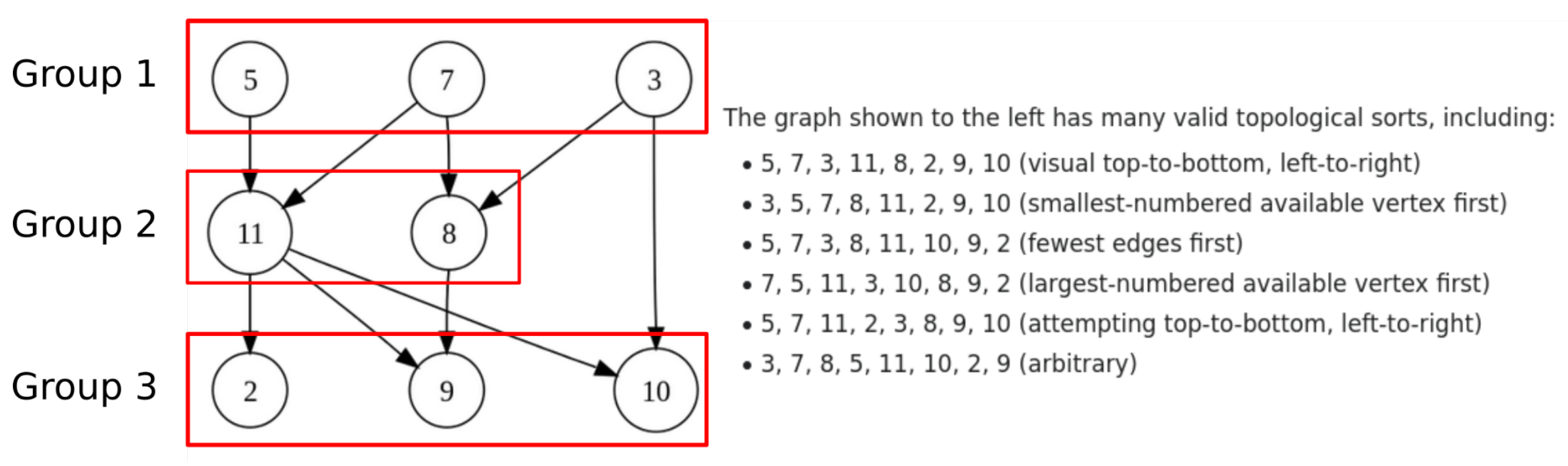
4.5. Topological Sorting
- Record intervals that denote MPI edges and program edges.
- Gather all intervals in rank 0.
- Sort them by start time (actually merge sorted arrays).
- Find overlapping program edges. In each group, the longest edge belongs to the critical path (Figure 5).
- Connect the longest program edges to each other.
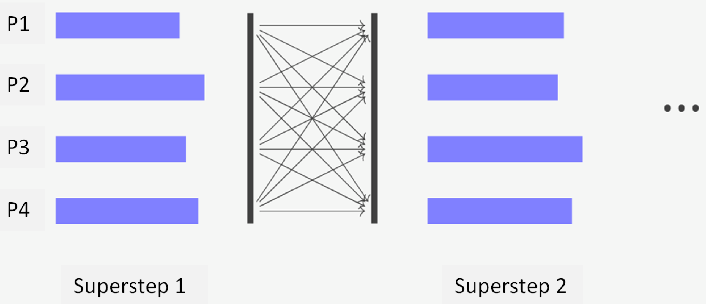
- Record intervals that denote MPI edges and program edges.
- Shuffle intervals between ranks. Each rank receives its own period of time.
- Merge shuffled arrays in each rank.
- Find overlapping program edges. In each group, the longest edge belongs to the critical path.
- Connect the longest program edges to each other.
- Gather all critical path segments in rank 0.
- Linear time O(n).
- Reliable: works even without cross-process edges.
- No graph: no graph cycles are possible, nor are infinite program loops.
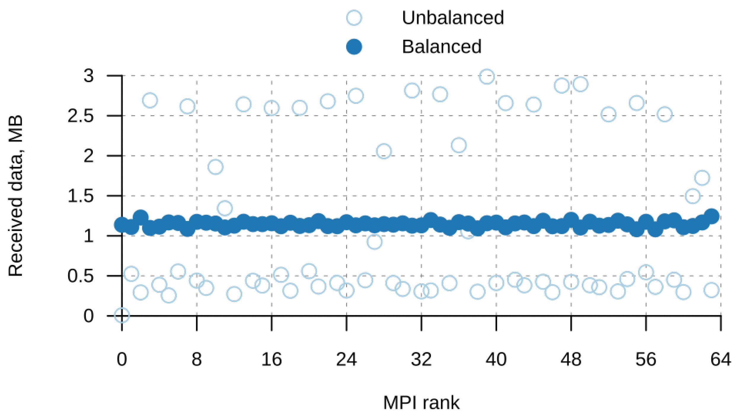
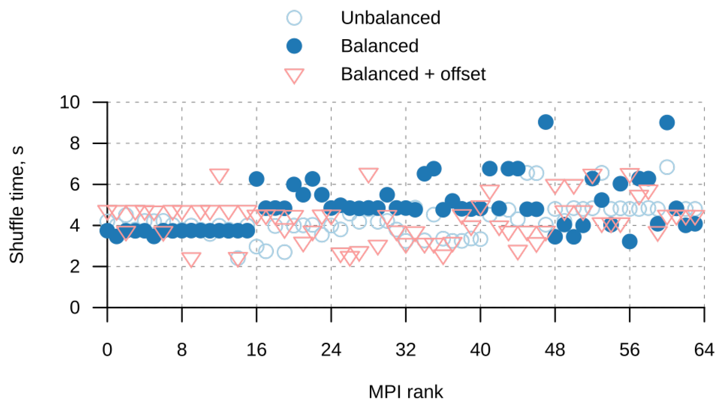
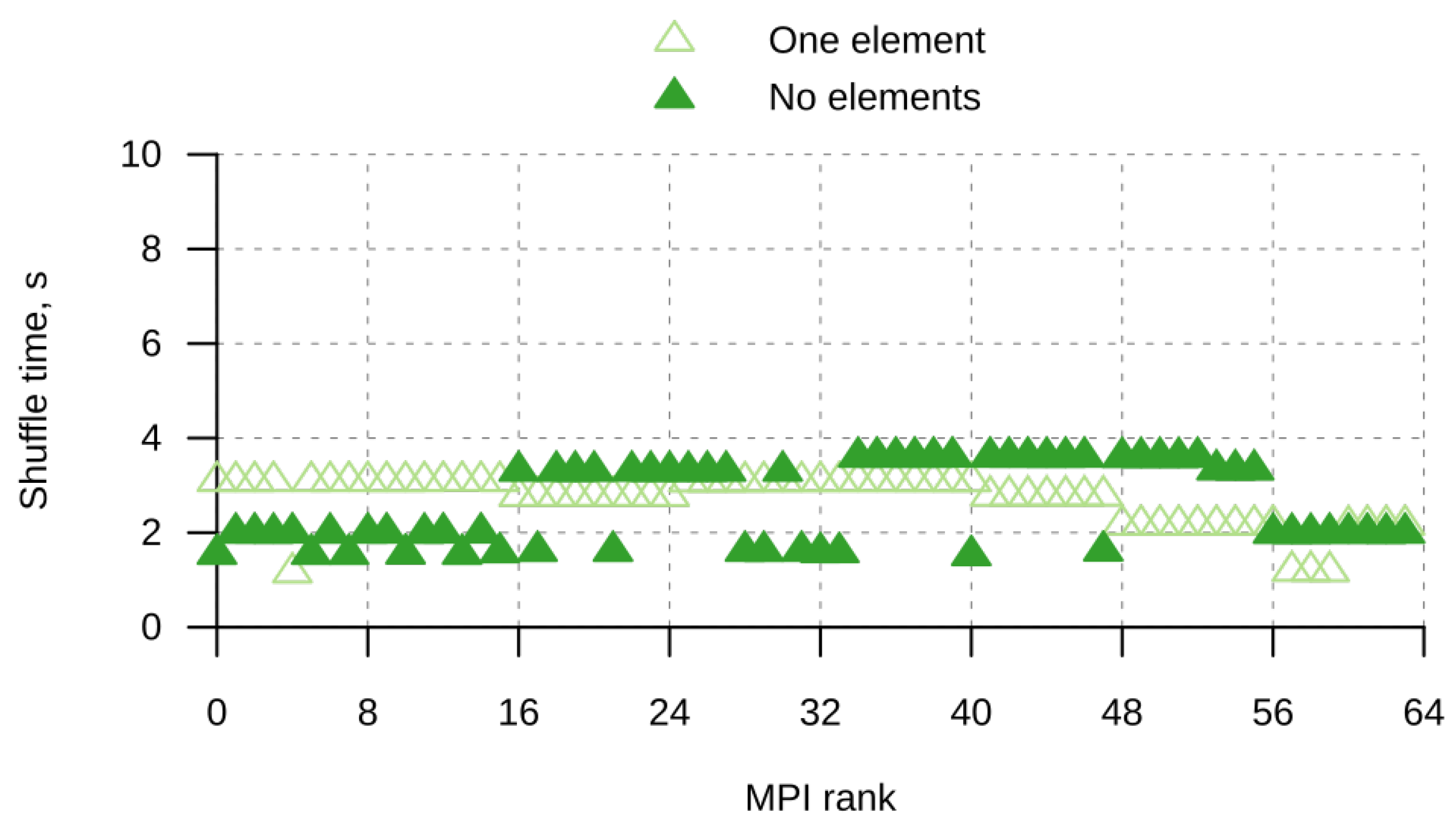
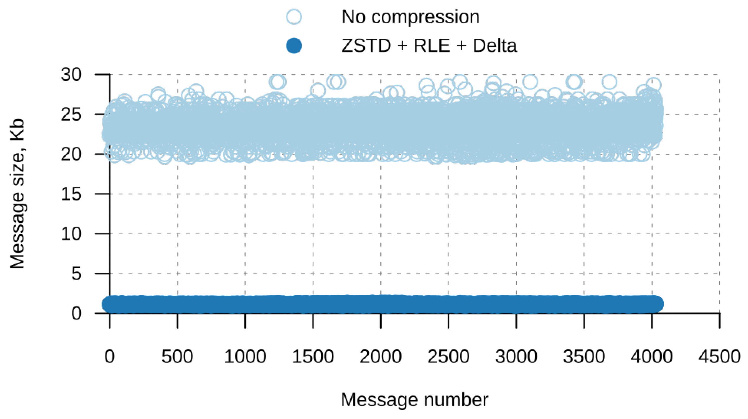
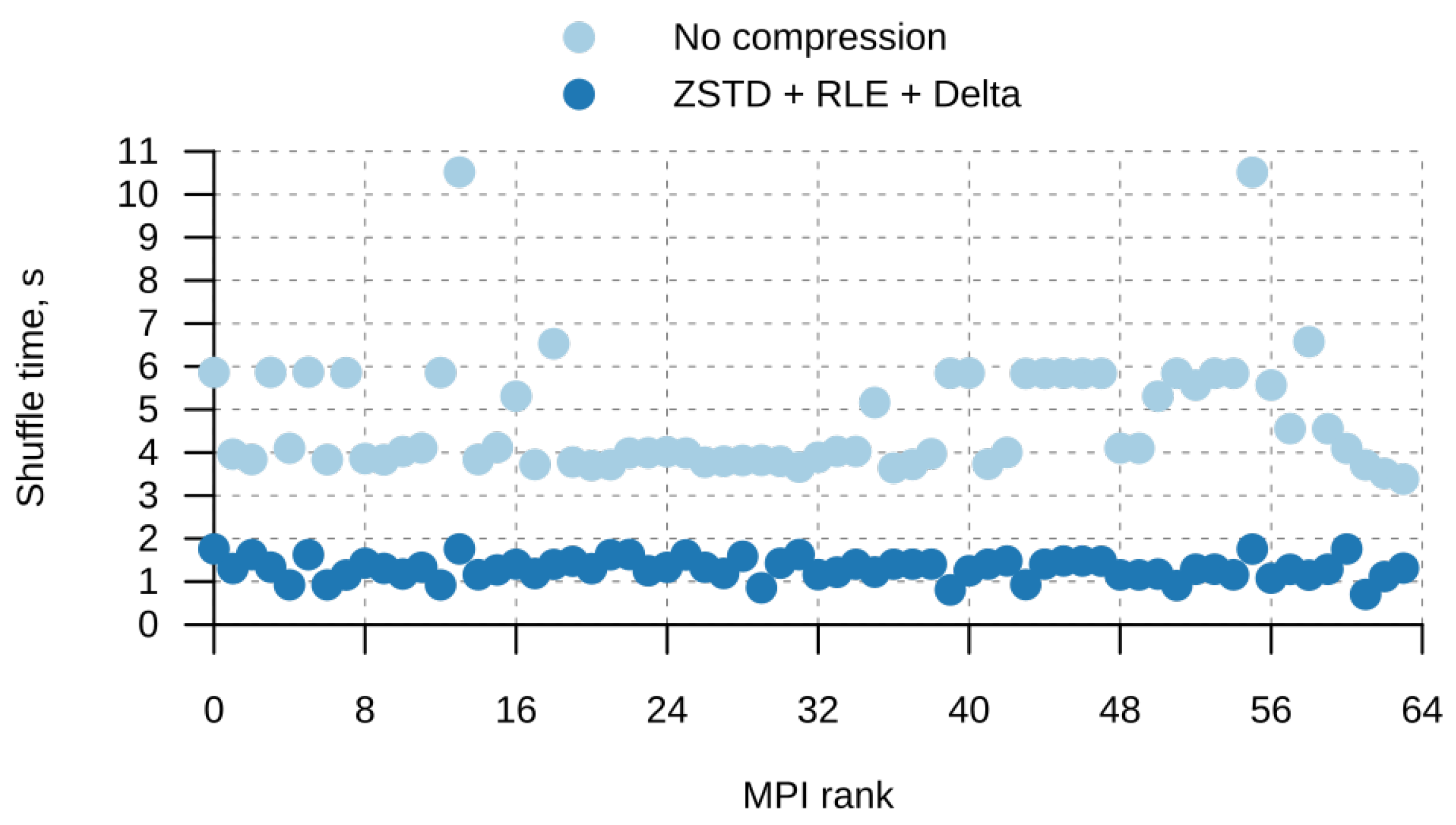
- Shuffle can be slow: need to transfer of the total size of the graph.
- Overlapping is good enough but not perfect: e.g., need to detect non-MPI_COMM_ WORLD communicators.
5. Profiling MPI Applications
5.1. Logging MPI Calls
5.2. Converting the Log Records to the Graph
- t_wait_before = t_start_max - t_start[i]
- t_wait_after = t_end[i] - t_end_min
- t_execution = t_end[i] - t_start[i] - t_wait_before - t_wait_after =
- = t_end_min - t_start_max
- imbalance = (t_wait_before + t_wait_after) / t_execution
- imbalance_call = (t_wait_before + t_wait_after) / t_execution
- imbalance_process = sum(t_wait_before + t_wait_after for each call)
- / (sum(t_execution for each call) + t_program_edges)
- imbalance_program =
- sum(t_wait_before + t_wait_after for each call and process)
- / (sum(t_execution for each call and process)
- + sum(t_program_edges for each process))
5.3. Synthetic Benchmarks
- Per-process statistics:
- rank program_time graph_time total_time total_execution_time
- 0 1.908003056 0.000988314 1.908991370 0.935452868
- 1 1.907246658 0.000208261 1.907454919 0.935452868
- 2 1.905164954 0.000214803 1.905379757 0.935452868
- 3 1.904170098 0.000349145 1.904519243 0.935452868
- rank total_wait_time imbalance num_calls num_nodes num_edges
- 0 0.018105627 0.019354932 3 8 13
- 1 1.344099347 1.436843472 3 6 13
- 2 1.335822343 1.427995347 3 6 13
- 3 1.332357843 1.424291793 3 6 13
- Total statistics:
- program_time=1.908642225
- graph_time=0.000349145
- total_time=1.908991370
- total_execution_time=3.741811472
- total_wait_time=4.030385160
- imbalance=1.077121386
- num_calls=12
- num_nodes=26
- num_edges=52
5.4. Time Synchronization
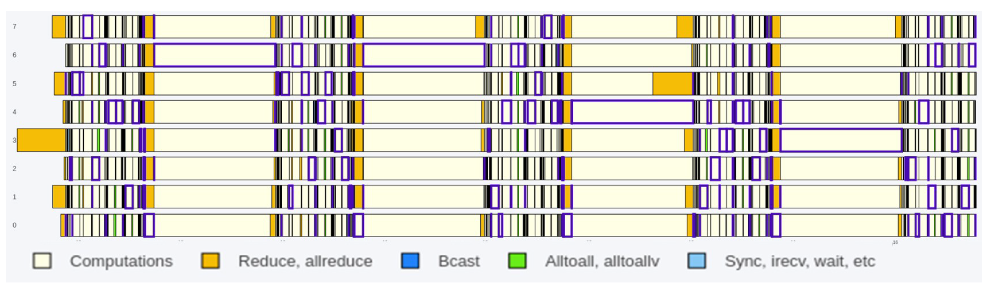
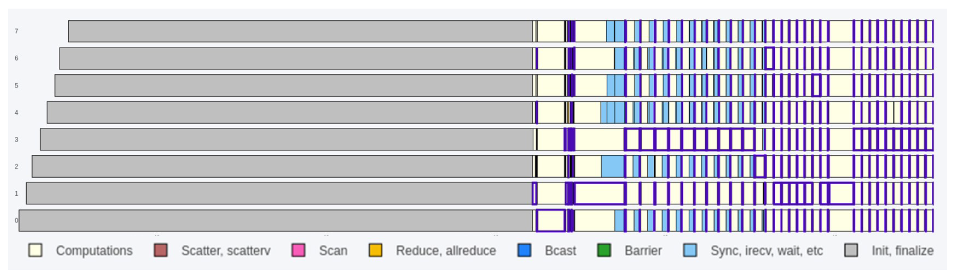
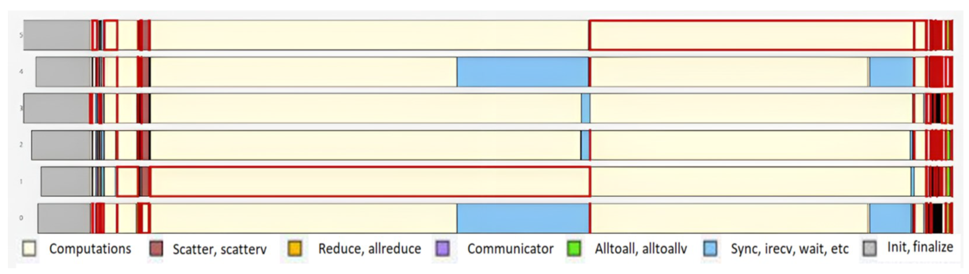
5.5. Visualization
5.6. Load Imbalance Estimation
5.6.1. Heuristic
5.6.2. Analytic
5.6.3. Pattern-Based
- Late Sender. This property refers to the amount of time lost when the MPI_Recv call is sent before the corresponding MPI_Send is executed.
- Late Receiver. This property applies to the opposite case. MPI_Send is blocked until the corresponding receive operation is called. This can happen for several reasons. Either the default implementation works in synchronous mode, or the size of the message being sent exceeds the available buffer space, and the operation is blocked until the data are transmitted to the recipient. The behavior is similar to MPI_SSend waiting for the message to be delivered. The downtime is measured, and the sum of all downtime periods is returned as a severity value.
- Messages in Wrong Order. This property concerns the problem of sending messages out of order. For example, the sender can send messages in a certain order, and the recipient can expect them to arrive in the reverse order.
- Wait at Barrier. This property corresponds to the downtime caused by the load imbalance when the barrier is called. The idle time is calculated by comparing the execution time of the process for each MPI_Barrier call. To work correctly, the implementation of this property requires the participation of all processes in each call of the collective barrier operation. The final value is simply the sum of all measured downtime periods.
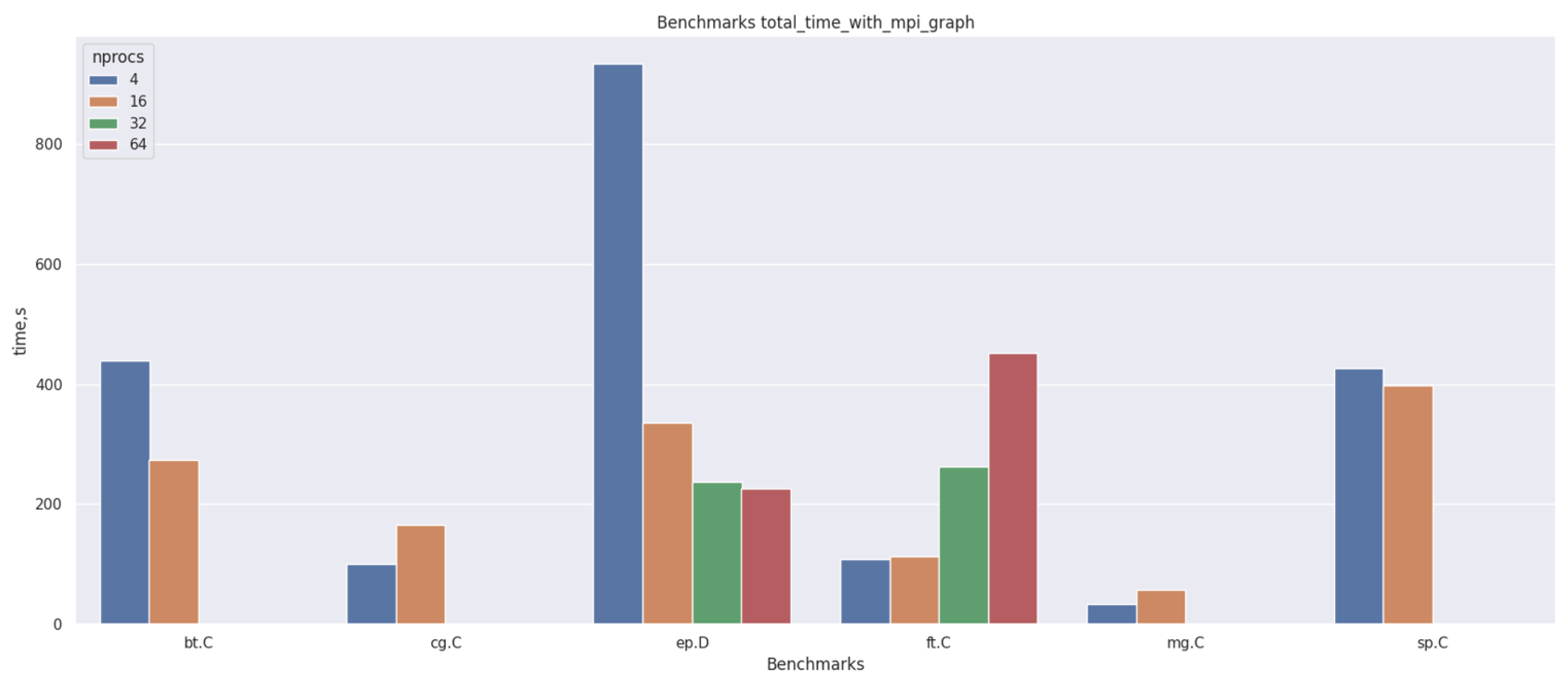
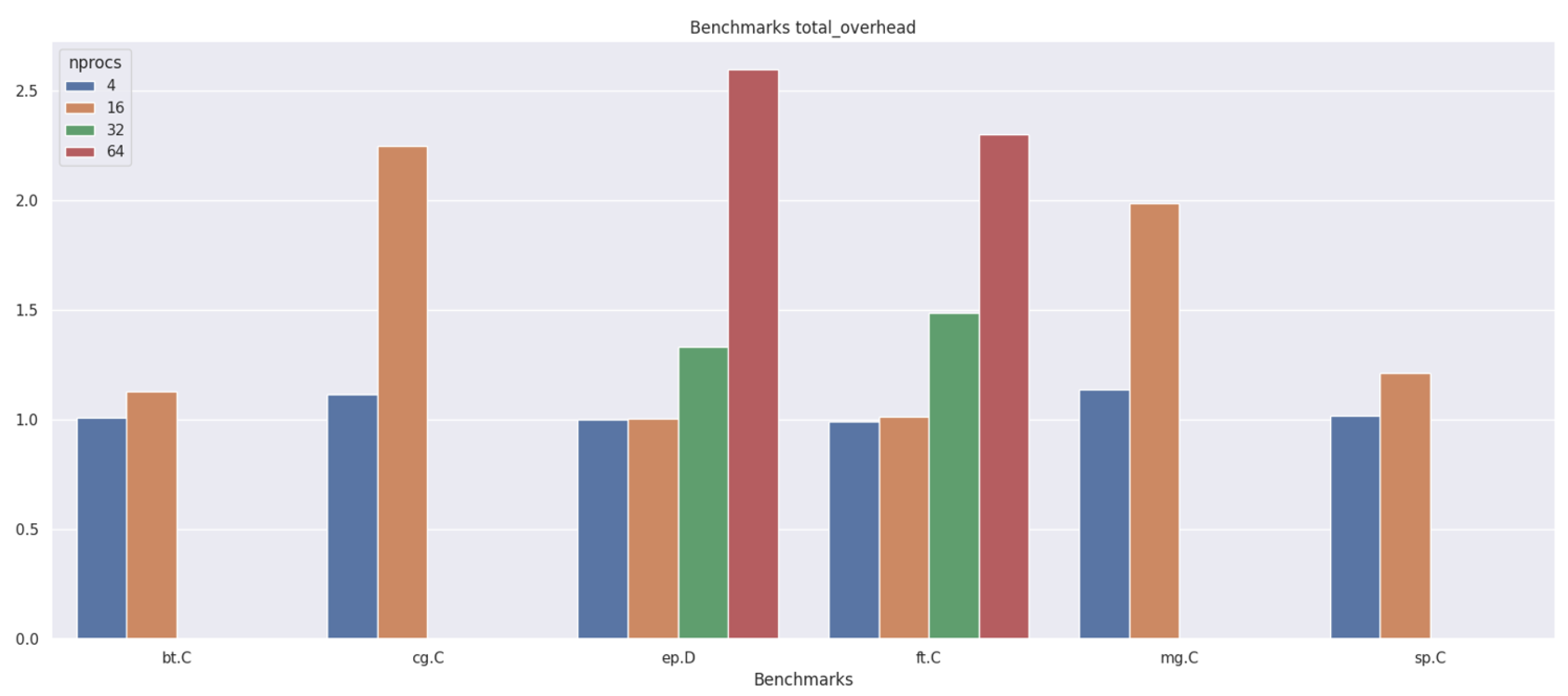
6. Benchmarking
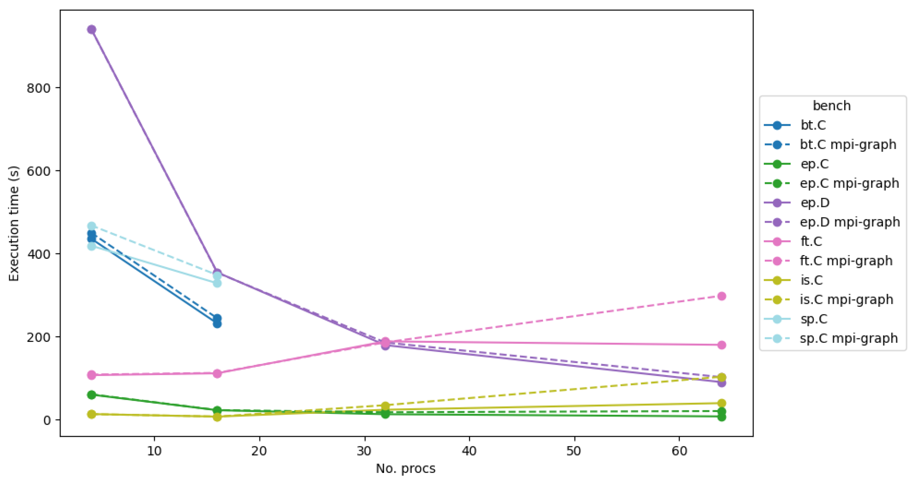
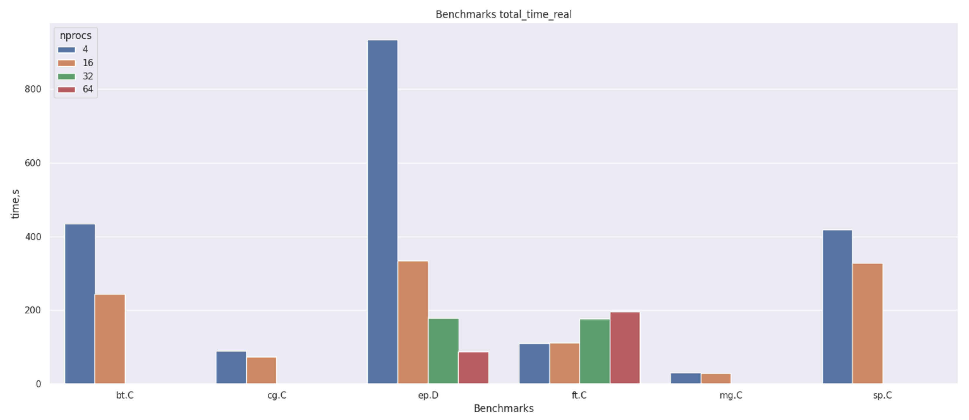
6.1. NAS Parallel Benchmarks
- Class S: small for quick test purposes;
- Class W: workstation size (a 1990s workstation; now likely too small)
- Classes A, B, and C: standard test problems; 4× size increase going from one class to the next;
- Classes D, E, and F: large test problems; 16× size increase from each of the previous classes.
- BT, SP—a square number of processes (1, 4, 9, ...);
- LU—2D (n1 × n2) process grid where n1/2 <= n2 <= n1;
- CG, FT, IS, MG—a power-of-two number of processes (1, 2, 4, ...);
- EP, DT—no special requirement.
- total run time with MPI call recording;
- total run time with MPI call recording + critical path finding;
- total run time without mpi-graph.
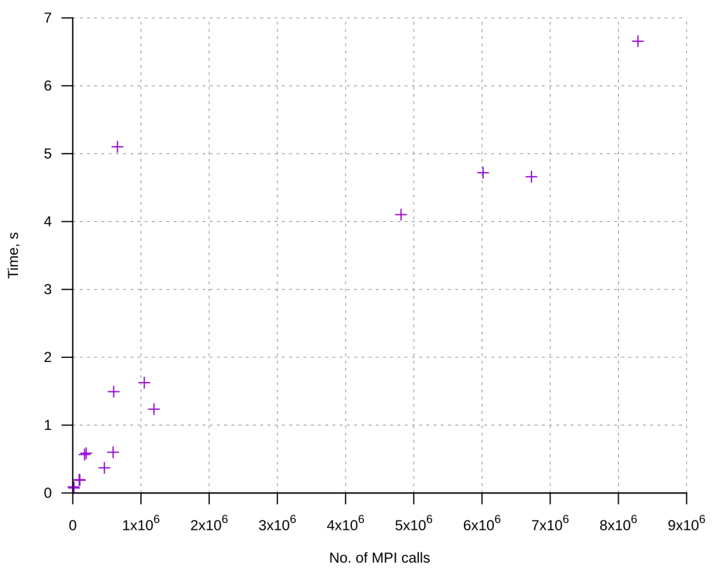
6.2. CP2K
6.3. OpenFOAM
- There are solvers, each of which is designed to solve a specific problem of continuum mechanics. Each solver has at least one tutorial that shows its use.
- There are utilities designed to perform tasks related to data manipulation. OpenFOAM comes with pre-/post-processing environments, each of which has its own utilities.
6.4. LAMMPS
6.5. MiniFE
6.6. Case Studies
7. Conclusions
Author Contributions
Funding
Data Availability Statement
Conflicts of Interest
References
- MPI Forum. Available online: https://www.mpi-forum.org/ (accessed on 18 October 2023).
- Schulz, M. Extracting Critical Path Graphs from MPI Applications. In Proceedings of the 2005 IEEE International Conference on Cluster Computing, Burlington, MA, USA, 27–30 September 2005. [Google Scholar] [CrossRef]
- Valiant, L.G. A bridging model for parallel computation. Commun. ACM 1990, 33, 103–111. [Google Scholar] [CrossRef]
- Bailey, D.H.; Schreiber, R.S.; Simon, H.D.; Venkatakrishnan, V.; Weeratunga, S.K.; Barszcz, E.; Barton, J.T.; Browning, D.S.; Carter, R.L.; Dagum, L.; et al. The NAS parallel benchmarks—Summary and preliminary results. In Proceedings of the 1991 ACM/IEEE Conference on Supercomputing—Supercomputing’91, Albuquerque, NM, USA, 18–22 November 1991; ACM Press: New York, NY, USA, 1991. [Google Scholar] [CrossRef]
- Kühne, T.D.; Iannuzzi, M.; Del Ben, M.; Rybkin, V.V.; Seewald, P.; Stein, F.; Laino, T.; Khaliullin, R.Z.; Schütt, O.; Schiffmann, F.; et al. CP2K: An electronic structure and molecular dynamics software package—Quickstep: Efficient and accurate electronic structure calculations. J. Chem. Phys. 2020, 152, 194103. [Google Scholar] [CrossRef] [PubMed]
- Thompson, A.P.; Aktulga, H.M.; Berger, R.; Bolintineanu, D.S.; Brown, W.M.; Crozier, P.S.; Veld, P.T.; Kohlmeyer, A.; Moore, S.G.; Nguyen, T.D.; et al. LAMMPS—A flexible simulation tool for particle-based materials modeling at the atomic, meso, and continuum scales. Comp. Phys. Comm. 2022, 271, 10817. [Google Scholar] [CrossRef]
- Chen, G.; Xiong, Q.; Morris, P.; Paterson, E.; Sergeev, A.; Wang, Y. OpenFOAM for computational fluid dynamics. N. Am. Math. Soc. 2014, 61, 354–363. [Google Scholar] [CrossRef]
- Lin, P.T.; Heroux, M.A.; Barrett, R.F.; Williams, A. Assessing a mini-application as a performance proxy for a finite element method engineering application. Concurr. Comput. Pract. Exp. 2015, 27, 5374–5389. [Google Scholar] [CrossRef]
- Yang, C.Q.; Miller, B.P. Critical Path Analysis for the Execution of Parallel and Distributed Programs. In Proceedings of the 8th International Conference on Distributed Computing Systems, San Jose, CA, USA, 13–17 June 1988; pp. 366–373. Available online: https://ftp.cs.wisc.edu/paradyn/papers/CritPath-ICDCS1988.pdf (accessed on 18 October 2023).
- Uehara, R.; Uno, Y. Efficient Algorithms for the Longest Path Problem. In Algorithms and Computation, Proceedings of the 15th International Symposium, ISAAC 2004, Hong Kong, China, 20–22 December 2004; Fleischer, R., Trippen, G., Eds.; Springer: Berlin/Heidelberg, Germay, 2005; Volume 15, pp. 871–883. [Google Scholar]
- Meyer, U.; Sanders, P. Δ-stepping: A parallelizable shortest path algorithm. J. Algorithms 2003, 49, 114–152. [Google Scholar] [CrossRef]
- Chakaravarthy, V.T.; Checconi, F.; Murali, P.; Petrini, F.; Sabharwal, Y. Scalable Single Source Shortest Path Algorithms for Massively Parallel Systems. IEEE Trans. Parallel Distrib. Syst. 2017, 28, 2031–2045. [Google Scholar] [CrossRef]
- Kranjvcevi’c, M.; Palossi, D.; Pintarelli, S. Parallel Delta-Stepping Algorithm for Shared Memory Architectures. arXiv 2016, arXiv:1604.02113. [Google Scholar]
- Zeng, W.; Church, R.L. Finding shortest paths on real road networks: The case for A*. Int. J. Geogr. Inf. Sci. 2009, 23, 531–543. [Google Scholar] [CrossRef]
- Alves, D.R.; Krishnakumar, M.S.; Garg, V.K. Efficient Parallel Shortest Path Algorithms. In Proceedings of the 2020 19th International Symposium on Parallel and Distributed Computing (ISPDC), Warsaw, Poland, 5–8 July 2020. [Google Scholar] [CrossRef]
- Chandy, K.M.; Misra, J. Distributed computation on graphs: Shortest path algorithms. Commun. ACM 1982, 25, 833–837. [Google Scholar] [CrossRef]
- Hollingsworth, J.K. Critical Path Profiling of Message Passing and Shared-Memory Programs. IEEE Trans. Parallel Distrib. Syst. 1998, 9, 1029–1040. [Google Scholar] [CrossRef]
- Dooley, I.; Arya, A.; Kalé, L.V. Detecting and using critical paths at runtime in message driven parallel programs. In Proceedings of the 2010 IEEE International Symposium on Parallel & Distributed Processing, Workshops and PhD Forum (IPDPSW), Atlanta, GA, USA, 19–23 April 2010; pp. 1–8. [Google Scholar]
- Böhme, D.; Wolf, F.A.; Geimer, M. Characterizing Load and Communication Imbalance in Large-Scale Parallel Applications. In Proceedings of the 2012 IEEE 26th International Parallel and Distributed Processing Symposium Workshops & PhD Forum, Shanghai, China, 21–25 May 2012; pp. 2538–2541. [Google Scholar]
- Geimer, M.; Wolf, F.; Wylie, B.; Ábrahám, E.; Becker, D.; Mohr, B. The SCALASCA performance toolset architecture. Concurr. Comput. Pract. Exp. 2010, 22, 702–719. [Google Scholar] [CrossRef]
- Grünewald, D.; Simmendinger, C. The GASPI API specification and its implementation GPI 2.0. In Proceedings of the 7th International Conference on PGAS Programming Models, Edinburgh, UK, 3–4 October 2013. [Google Scholar]
- Herold, C.; Krzikalla, O.; Knüpfer, A. Optimizing One-Sided Communication of Parallel Applications Using Critical Path Methods. In Proceedings of the 2017 IEEE International Parallel and Distributed Processing Symposium Workshops (IPDPSW), Orlando, FL, USA, 29 May–2 June 2017; pp. 567–576. [Google Scholar] [CrossRef]
- Chen, J.; Clapp, R.M. Critical-path candidates: Scalable performance modeling for MPI workloads. In Proceedings of the 2015 IEEE International Symposium on Performance Analysis of Systems and Software (ISPASS), Philadelphia, PA, USA, 29–31 March 2015; pp. 1–10. [Google Scholar]
- Nguyen, D.D.; Karavanic, K.L. Workflow Critical Path: A data-oriented critical path metric for Holistic HPC Workflows. BenchCounc. Trans. Benchmarks Stand. Eval. 2021, 1, 100001. [Google Scholar] [CrossRef]
- Shatalin, A.; Slobodskoy, V.; Fatin, M. Root Causing MPI Workloads Imbalance Issues via Scalable MPI Critical Path Analysis. In Supercomputing: 8th Russian Supercomputing Days, RuSCDays 2022, Moscow, Russia, September 26–27, 2022, Revised Selected Papers; Voevodin, V., Sobolev, S., Yakobovskiy, M., Shagaliev, R., Eds.; Springer International Publishing: Cham, Switzerland, 2022; pp. 501–521. [Google Scholar]
- Fieger, K.; Balyo, T.; Schulz, C.; Schreiber, D. Finding optimal longest paths by dynamic programming in parallel. In Proceedings of the Twelfth Annual Symposium on Combinatorial Search, Napa, CA, USA, 16–17 July 2019. [Google Scholar]
- Raggi, M. Finding long simple paths in a weighted digraph using pseudo-topological orderings. arXiv 2016, arXiv:1609.07450. [Google Scholar]
- Portugal, D.; Antunes, C.H.; Rocha, R. A study of genetic algorithms for approximating the longest path in generic graphs. In Proceedings of the 2010 IEEE International Conference on Systems, Man and Cybernetics, Istanbul, Turkey, 10–13 October 2010; pp. 2539–2544. [Google Scholar] [CrossRef]
- Pjesivac-Grbovic, J.; Angskun, T.; Bosilca, G.; Fagg, G.; Gabriel, E.; Dongarra, J. Performance Analysis of MPI Collective Operations. In Proceedings of the 19th IEEE International Parallel and Distributed Processing Symposium, Denver, CO, USA, 4–8 April 2005. [Google Scholar] [CrossRef]
- Pješivac-Grbović, J.; Angskun, T.; Bosilca, G.; Fagg, G.E.; Gabriel, E.; Dongarra, J.J. Performance analysis of MPI collective operations. Clust. Comput. 2007, 10, 127–143. [Google Scholar] [CrossRef]
- Saif, T.; Parashar, M. Understanding the Behavior and Performance of Non-blocking Communications in MPI. In Lecture Notes in Computer Science; Springer: Berlin/Heidelberg, Germany, 2004; pp. 173–182. [Google Scholar] [CrossRef]
- Hoefler, T.; Lumsdaine, A.; Rehm, W. Implementation and performance analysis of non-blocking collective operations for MPI. In Proceedings of the 2007 ACM/IEEE Conference on Supercomputing—SC’07, Reno, NV, USA, 10–16 November 2007; ACM Press: New York, NY, USA, 2007. [Google Scholar] [CrossRef]
- Ueno, K.; Suzumura, T. Highly scalable graph search for the Graph500 benchmark. In Proceedings of the 21st International Symposium on High-Performance Parallel and Distributed Computing—HPDC’12, Online, 21–25 June 2012; ACM Press: New York, NY, USA, 2012. [Google Scholar] [CrossRef]
- Dijkstra, E.W. A note on two problems in connexion with graphs. Numer. Math. 1959, 1, 269–271. [Google Scholar] [CrossRef]
- Kahn, A.B. Topological sorting of large networks. Commun. ACM 1962, 5, 558–562. [Google Scholar] [CrossRef]
- Aguilar, X. Performance Monitoring, Analysis, and Real-Time Introspection on Large-Scale Parallel Systems. Ph.D. Thesis, KTH Royal Institute of Technology, Stockholm, Sweden, 2020. [Google Scholar]
- Garcia, M.; Corbalan, J.; Labarta, J. LeWI: A runtime balancing algorithm for nested parallelism. In Proceedings of the 2009 International Conference on Parallel Processing, Vienna, Austria, 22–25 September 2009; pp. 526–533. [Google Scholar]
- Arzt, P.; Fischler, Y.; Lehr, J.P.; Bischof, C. Automatic low-overhead load-imbalance detection in MPI applications. In European Conference on Parallel Processing; Springer: Berlin/Heidelberg, Germany, 2021; pp. 19–34. [Google Scholar]
- Pearce, O.; Gamblin, T.; De Supinski, B.R.; Schulz, M.; Amato, N.M. Quantifying the effectiveness of load balance algorithms. In Proceedings of the 26th ACM International Conference on Supercomputing, Venice, Italy, 25–29 June 2012; pp. 185–194. [Google Scholar]
- Tallent, N.R.; Adhianto, L.; Mellor-Crummey, J.M. Scalable identification of load imbalance in parallel executions using call path profiles. In Proceedings of the SC’10: 2010 ACM/IEEE International Conference for High Performance Computing, Networking, Storage and Analysis, New Orleans, LA, USA, 13–19 November 2010; pp. 1–11. [Google Scholar]
- Schmitt, F.; Stolle, J.; Dietrich, R. CASITA: A tool for identifying critical optimization targets in distributed heterogeneous applications. In Proceedings of the 2014 43rd International Conference on Parallel Processing Workshops, Minneapolis, MN, USA, 9–12 September 2014; pp. 186–195. [Google Scholar]
- Wolf, F.; Mohr, B. Automatic performance analysis of MPI applications based on event traces. In European Conference on Parallel Processing; Springer: Berlin/Heidelberg, Germany, 2000; pp. 123–132. [Google Scholar]
- Wolf, F.; Mohr, B. Automatic performance analysis of hybrid MPI/OpenMP applications. J. Syst. Archit. 2003, 49, 421–439. [Google Scholar] [CrossRef]
- Schmitt, F.; Dietrich, R.; Juckeland, G. Scalable critical path analysis for hybrid MPI-CUDA applications. In Proceedings of the 2014 IEEE International Parallel & Distributed Processing Symposium Workshops, Phoenix, AZ, USA, 19–23 May 2014; pp. 908–915. [Google Scholar]
- Hermanns, M.A.; Miklosch, M.; Böhme, D.; Wolf, F. Understanding the formation of wait states in applications with one-sided communication. In Proceedings of the 20th European MPI Users’ Group Meeting, Madrid, Spain, 15–18 September 2013; pp. 73–78. [Google Scholar]
- OpenFOAM Tutorial, pitzDailyExptInlet Case Code Repository. Available online: https://github.com/OpenFOAM/OpenFOAM-9/tree/master/tutorials//incompressible/simpleFoam/pitzDailyExptInlet (accessed on 18 October 2023).
- LAMMPS Benchmarks. Available online: https://docs.lammps.org/Speed_bench.html (accessed on 18 October 2023).


| Benchmark | Name | Description | Problem Sizes and Parameters (Class C) |
|---|---|---|---|
| MG | Multi-grid on a sequence of meshes, long- and short-distance communication, memory intensive | Approximation of the solution of a three-dimensional discrete Poisson equation using the V-cycle multigrid method. | grid size: 512 × 512 × 512 no. of iterations: 20 |
| CG | Conjugate gradient, irregular memory access and communication | Approximation to the smallest eigenvalue of a large sparse, symmetric positive-definite matrix using inverse iteration together with the conjugate gradient method as a subroutine for solving linear systems of algebraic equations. | no. of rows: 150,000 no. of nonzeros: 15 no. of iterations: 75 eigenvalue shift: 110 |
| FT | Discrete 3D fast Fourier Transform all-to-all communication | Solving a three-dimensional partial differential equation using the Fast Fourier Transform (FFT). | grid size: 512 × 512 × 512 no. of iterations: 20 |
| IS | Integer sort, random memory access | Sorting small integers using pocket sorting. | no. of keys: key max. value: |
| EP | Embarrassingly Parallel | Generation of independent normally distributed random variables using Marsaglia polar method. | no. of random-number pairs: |
| BT | Block tri-diagonal solver | Solves a synthetic system of nonlinear diffs. partial differential equations (a 3-dimensional system of Navier–Stokes equations for a compressible liquid or gas) using a three-block tridiagonal scheme with the method of variable directions (BT), a scalar five-diagonal scheme (SP), and a method of symmetric sequential upper relaxation (SSOR algorithm, LU problem). | grid size: 162 × 162 × 162 no. of iterations: 200 time step: 0.0001 |
| SP | Scalar penta-diagonal solver | Solution of the heat equation taking into account diffusion and convection in a cube. The heat source is mobile, the grid is irregular, and changes every 5 steps. | grid size: 162 × 162 × 162 no. of iterations: 400 time step: 0.00067 |
| LU | Lower-upper Gauss–Seidel solver | Same problem as SP, but the method is different. | grid size: 162 × 162 × 162 no. of iterations: 250 time step: 2.0 |
| Benchmark | Nprocesses | Nnodes | Tasks-per-Node | Rel. Overhead (No Compression) | Rel. Overhead (Compression) |
|---|---|---|---|---|---|
| ep.C | 4 | 1 | 4 | 0.02 | 0.01 |
| ep.C | 16 | 2 | 8 | 0 | 0.01 |
| ep.C | 32 | 4 | 8 | 0.09 | 0.02 |
| ep.C | 64 | 8 | 8 | 0.44 | 0.05 |
| is.C | 4 | 1 | 4 | 0 | 0 |
| is.C | 16 | 2 | 8 | 0.02 | 0.001 |
| is.C | 32 | 4 | 8 | 0.19 | 0.06 |
| is.C | 64 | 8 | 8 | 0.06 | 0 |
| lu.C | 4 | 1 | 4 | 0 | 0.01 |
| lu.C | 16 | 2 | 8 | 0.06 | 0.02 |
| lu.C | 32 | 4 | 8 | 0.10 | 0.04 |
| lu.C | 64 | 8 | 8 | 0.16 | 0.09 |
| mg.C | 4 | 1 | 4 | 0 | 0.01 |
| mg.C | 16 | 2 | 8 | 0.04 | 0 |
| mg.C | 32 | 4 | 8 | 0.14 | 0.02 |
| mg.C | 64 | 8 | 8 | 0.25 | 0.06 |
| No. of Nodes | No. of Processes per Node | Program Time, s | MPI-Graph Time, s | Overhead, % |
|---|---|---|---|---|
| 2 | 2 | 432.61 | 0.024 | 0.01% |
| 4 | 4 | 150.25 | 0.21 | 0.14% |
| 8 | 8 | 100.78 | 1.52 | 1.49% |
| No. of Nodes | No. of Processes per Node | Program Time, s | MPI-Graph Time, s | Overhead, % |
|---|---|---|---|---|
| 1 | 8 | 31.51 | 0.001 | 0.00% |
| 2 | 8 | 15.89 | 0.010 | 0.06% |
| 4 | 8 | 8.07 | 0.069 | 0.85% |
| 8 | 8 | 5.19 | 0.059 | 1.14% |
| No. of Nodes | No. of Processes per Node | Program Time, s | MPI-Graph Time, s | Overhead, % |
|---|---|---|---|---|
| 1 | 8 | 7.18 | 0.16 | 2.23% |
| 2 | 8 | 16.96 | 0.17 | 1.03% |
| 4 | 8 | 18.91 | 0.11 | 0.57% |
| 8 | 8 | 26.60 | 0.13 | 0.48% |
| No. of Nodes | No. of Processes per Node | Program Time, s | MPI-Graph Time, s | Overhead, % |
|---|---|---|---|---|
| 1 | 8 | 21.56 | 0.03 | 0.14% |
| 2 | 8 | 14.82 | 0.13 | 0.89% |
| 4 | 8 | 16.81 | 0.37 | 2.14% |
| 8 | 8 | 8.43 | 0.83 | 8.94% |
| No. of Nodes | No. of Processes per Node | Program Time, s | MPI-Graph Time, s | Overhead, % |
|---|---|---|---|---|
| 2 | 2 | 198.51 | 0.09 | 0.05% |
| 4 | 4 | 113.77 | 0.38 | 0.33% |
| 8 | 8 | 105.89 | 0.24 | 0.23% |
| No. of Nodes | No. of Processes per Node | Program Time, s | MPI-Graph Time, s | Overhead, % |
|---|---|---|---|---|
| 2 | 2 | 260.86 | 0.51 | 0.19% |
| 4 | 4 | 92.11 | 1.66 | 1.77% |
| 8 | 8 | 58.76 | 5.34 | 8.33% |
| Test Case | Compression | Threshold, s |
|---|---|---|
| bt.C | no | 0 |
| ep.C | no | 0 |
| is.C | no | 0 |
| mg.C | no | 0 |
| ft.C | no | 0 |
| lu.C | yes (min. level) | 0 |
| Acronym | Meaning |
|---|---|
| ssmp | Single process + symmetric multiprocessor (OpenMP) |
| sdbg | ssmp + debug settings |
| psmp | Parallel (MPI) + symmetric multiprocessor (OpenMP) |
| popt | psmp + optimized |
| pdbg | psmp + debug settings |
| No. of Nodes | No. of Processes per Node | Program Time, s | MPI-Graph Time, s | Overhead, % |
|---|---|---|---|---|
| 2 | 2 | 12.24 | 0.011 | 0.09% |
| 4 | 4 | 24.74 | 0.027 | 0.11% |
| 8 | 8 | 121.92 | 0.371 | 0.30% |
| 10 | 8 | 142.55 | 4.162 | 2.84% |
| Test Case | No. of Iterations | Compression | Threshold, s |
|---|---|---|---|
| fayalite | 10 | yes (min level) | 0 |
| No. of Nodes | No. of Processes per Node | Program Time, s | MPI-Graph Time, s | Overhead, % |
|---|---|---|---|---|
| 2 | 2 | 70.56 | 1.47 | 2.05% |
| 4 | 4 | 104.35 | 2.98 | 2.79% |
| 8 | 8 | 219.03 | 9.62 | 4.21% |
| 10 | 8 | 230.47 | 10.02 | 4.18% |
| Test Case | No. of Iterations | Compression | Threshold, s |
|---|---|---|---|
| pitzDailyExptInlet | 1000 | yes (min level) | 0.001 |
| No. of Nodes | No. of Processes per Node | Program Time, s | MPI-Graph Time, s | Overhead, % |
|---|---|---|---|---|
| 2 | 2 | 125.92 | 0.28 | 0.22% |
| 4 | 4 | 63.52 | 0.49 | 0.76% |
| 8 | 8 | 35.31 | 1.53 | 4.16% |
| 10 | 8 | 49.33 | 2.64 | 5.08% |
| Test Case | No. of Iterations | Compression | Threshold, s |
|---|---|---|---|
| in.lj | 10,000 | yes (min level) | 0.001 |
| No. of Nodes | No. of Processes per Node | Program Time, s | MPI-Graph Time, s | Overhead, % |
|---|---|---|---|---|
| 2 | 2 | 137.73 | 0.05 | 0.03% |
| 4 | 4 | 52.43 | 0.22 | 0.42% |
| 8 | 8 | 39.78 | 1.00 | 2.44% |
| 10 | 8 | 36.38 | 2.35 | 6.06% |
| Test Case | Compression | Threshold, s |
|---|---|---|
| nx = 300 ny = 300 nz = 300 | yes (max level) | 0 |
Disclaimer/Publisher’s Note: The statements, opinions and data contained in all publications are solely those of the individual author(s) and contributor(s) and not of MDPI and/or the editor(s). MDPI and/or the editor(s) disclaim responsibility for any injury to people or property resulting from any ideas, methods, instructions or products referred to in the content. |
© 2023 by the authors. Licensee MDPI, Basel, Switzerland. This article is an open access article distributed under the terms and conditions of the Creative Commons Attribution (CC BY) license (https://creativecommons.org/licenses/by/4.0/).
Share and Cite
Korkhov, V.; Gankevich, I.; Gavrikov, A.; Mingazova, M.; Petriakov, I.; Tereshchenko, D.; Shatalin, A.; Slobodskoy, V. Finding Bottlenecks in Message Passing Interface Programs by Scalable Critical Path Analysis. Algorithms 2023, 16, 505. https://doi.org/10.3390/a16110505
Korkhov V, Gankevich I, Gavrikov A, Mingazova M, Petriakov I, Tereshchenko D, Shatalin A, Slobodskoy V. Finding Bottlenecks in Message Passing Interface Programs by Scalable Critical Path Analysis. Algorithms. 2023; 16(11):505. https://doi.org/10.3390/a16110505
Chicago/Turabian StyleKorkhov, Vladimir, Ivan Gankevich, Anton Gavrikov, Maria Mingazova, Ivan Petriakov, Dmitrii Tereshchenko, Artem Shatalin, and Vitaly Slobodskoy. 2023. "Finding Bottlenecks in Message Passing Interface Programs by Scalable Critical Path Analysis" Algorithms 16, no. 11: 505. https://doi.org/10.3390/a16110505
APA StyleKorkhov, V., Gankevich, I., Gavrikov, A., Mingazova, M., Petriakov, I., Tereshchenko, D., Shatalin, A., & Slobodskoy, V. (2023). Finding Bottlenecks in Message Passing Interface Programs by Scalable Critical Path Analysis. Algorithms, 16(11), 505. https://doi.org/10.3390/a16110505