GPU Algorithms for Structured Sparse Matrix Multiplication with Diagonal Storage Schemes ^†

Abstract

Matrix–matrix multiplication is of singular importance in linear algebra operations with a multitude of applications in scientific and engineering computing. Data structures for storing matrix elements are designed to minimize overhead information as well as to optimize the operation count. In this study, we utilize the notion of the compact diagonal storage method (CDM), which builds upon the previously developed diagonal storage—an orientation-independent uniform scheme to store the nonzero elements of a range of matrices. This study exploits both these storage schemes and presents efficient GPU-accelerated parallel implementations of matrix multiplication when the input matrices are banded and/or structured sparse. We exploit the data layouts in the diagonal storage schemes to expose a substantial amount of fine-grained parallelism and effectively utilize the GPU shared memory to improve the locality of data access for numerical calculations. Results from an extensive set of numerical experiments with the aforementioned types of matrices demonstrate orders-of-magnitude speedups compared with the sequential performance.

1. Introduction

The ubiquitous matrix multiplication operation is an essential component of many problems arising in combinatorial and scientific computing. It is considered an intermediate step in a myriad of scientific, graph, and engineering applications including computer graphics, network theory, algebraic multigrid solvers, triangle counting, multisource breadth-first searching, shortest path problems, colored intersecting, subgraph matching, and quantized neural networks [1,2,3,4,5,6]. The data structures for storing large matrices optimize the memory used for storage and the performance of the multiplication operation. However, the design and selection of storage formats for matrices depend on several issues, like intended applications, functions to be implemented, and the structures of the matrices [7].

For the multiplication of two general dense matrices, it is common to store two-dimensional matrices by rows (like row-major order used in C/C++ 20 and Java 18) or by columns (column-major order used in FORTRAN 2018 and MATLAB R2023b). There exist a wide variety of storage formats to match various features of sparse matrices [8]. In the case of general sparse matrices, a traditional triple-loop matrix multiplication algorithm employs row-wise access with Compact Row Storage (CRS) or transposed access with Compact Column Storage (CCS). However, numerical solutions to partial differential equations often give rise to a class of structured sparse matrices in engineering applications known as banded/band matrices. When exploited, the banded structures of these matrices provide some advantages, in contrast to unstructured sparse matrices, as they reduce not only the number of arithmetic operations but also the storage of and cache-friendly access to the matrix elements [9]. The storage of the subdiagonals and superdiagonals of banded matrices in consecutive memory locations supports a compact storage format, providing a trade-off between minimizing storage and enabling a cache-friendly access pattern of the matrix elements [10].

Compared to either CCS or CRS for the vectorized matrix multiplication of banded matrices, Madsen et al. [11] demonstrated that storage via diagonals and direct usage of these diagonals as vectors in matrix multiplication can be advantageous and computationally effective. Additionally, CCS/CRS does not allow transposes of matrices to be readily available for use in vector forms. Similarly, Tsao and Turnbull [12] demonstrated through numerical experiments that the algorithm developed by Madsen et al. was capable of rewriting the multiplication such that contagious elements from the diagonals were multiplied rather than the elements from rows and columns. This alleviated the problem associated with irregular access and yielded significant improvements in terms of both storage cost and computation time for the multiplication of matrices with smaller bandwidths.

Researchers [13] also focused on improving the performance of linear algebra operations on a variety of modern many-core architectures. The inherent challenging issues of linear algebra computations (e.g., load balancing, the irregular nature of the computations, and difficulty in predicting the output size) are further complicated in many-core systems’ (e.g., GPU) architectural constraints (e.g., memory access, limited shared memory, strict SIMD, and thread execution). Benner et al. [14] identified a number of reasons for the progressive adoption of modern graphics processing units (GPUs). These reasons include the following: (i) the availability of an application programming interface (e.g., CUDA [15], OpenCL [16]), (ii) affordable price, (iii) notable raw performance improvement, and (iv) favorable power–performance ratio. In particular, for dense matrix multiplication, many studies [17,18,19] demonstrated the benefits of GPU computing for achieving high efficiency.

Sparse matrices vary greatly in terms of their sizes, densities, and structures. Therefore, special storage formats were reasonably sought for matrices with certain characteristics to obtain better performance in terms of computation time. The current study utilizes a novel compact diagonal storage structure adopted from the work of Hossain and Mahmud [20]. The advantages of their approach along with efficient cache usage and reduced storage requirements, as identified in [21], are (i) a one-dimensional storage alternative without padding improving the previous storage schemes that utilized a two-dimensional array to store the diagonals, (ii) efficient scaling over the increased bandwidth of the matrices and the parallel processing of the independent diagonal calculations, and (iii) space efficiency for diagonal matrices and stride-1 access to the matrix elements avoiding any form of indirect referencing required in CRS and CCS. However, the above study did not address the multiplication operations using the transpose of dense matrices and special sparse matrices where the nonzeros are confined to diagonals while these nonzero diagonals are distributed arbitrarily in the matrix. An example of the sparsity pattern of a matrix is shown in Figure 1. We call these sparse matrices structured sparse matrices.

Note that, for the rest of this study, we refer to the compact diagonal storage structure as CDM and its predecessor, developed by Hossain and Mahmud, as the HM storage structure.

The objectives of this study are to develop GPU algorithms and explore the impact of this novel storage scheme including the aforementioned diagonal storage scheme [20] (i.e., CDM and HM, respectively) on the product of (i) banded matrices with varying bandwidth and (ii) structured sparse matrices with varying numbers of diagonals.

The contributions of the current study can be summarized as follows:

• We introduce GPU algorithms, for the first time, to multiply banded and structured sparse matrices, where the sparse matrices are stored as the CDM and HM schemes, respectively;
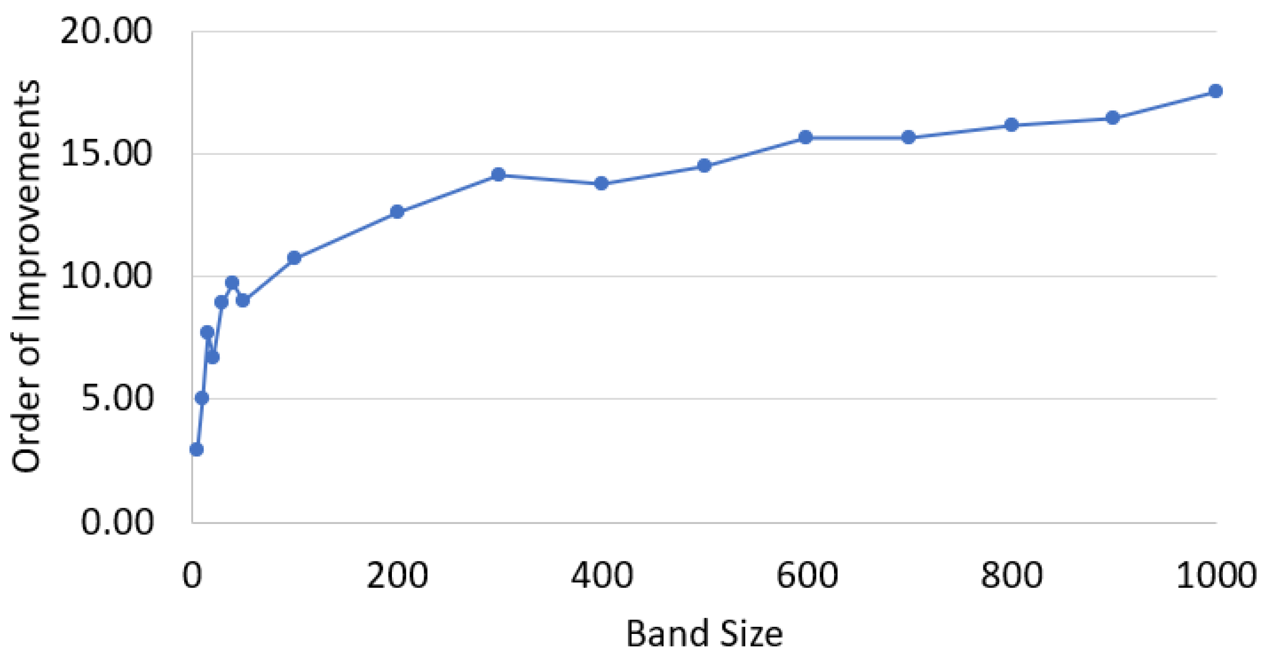
• Explore the performance of both the CDM and HM storage schemes in the multiplication of banded matrices with varying bandwidth and of structured sparse matrices with varying numbers of diagonals, respectively;
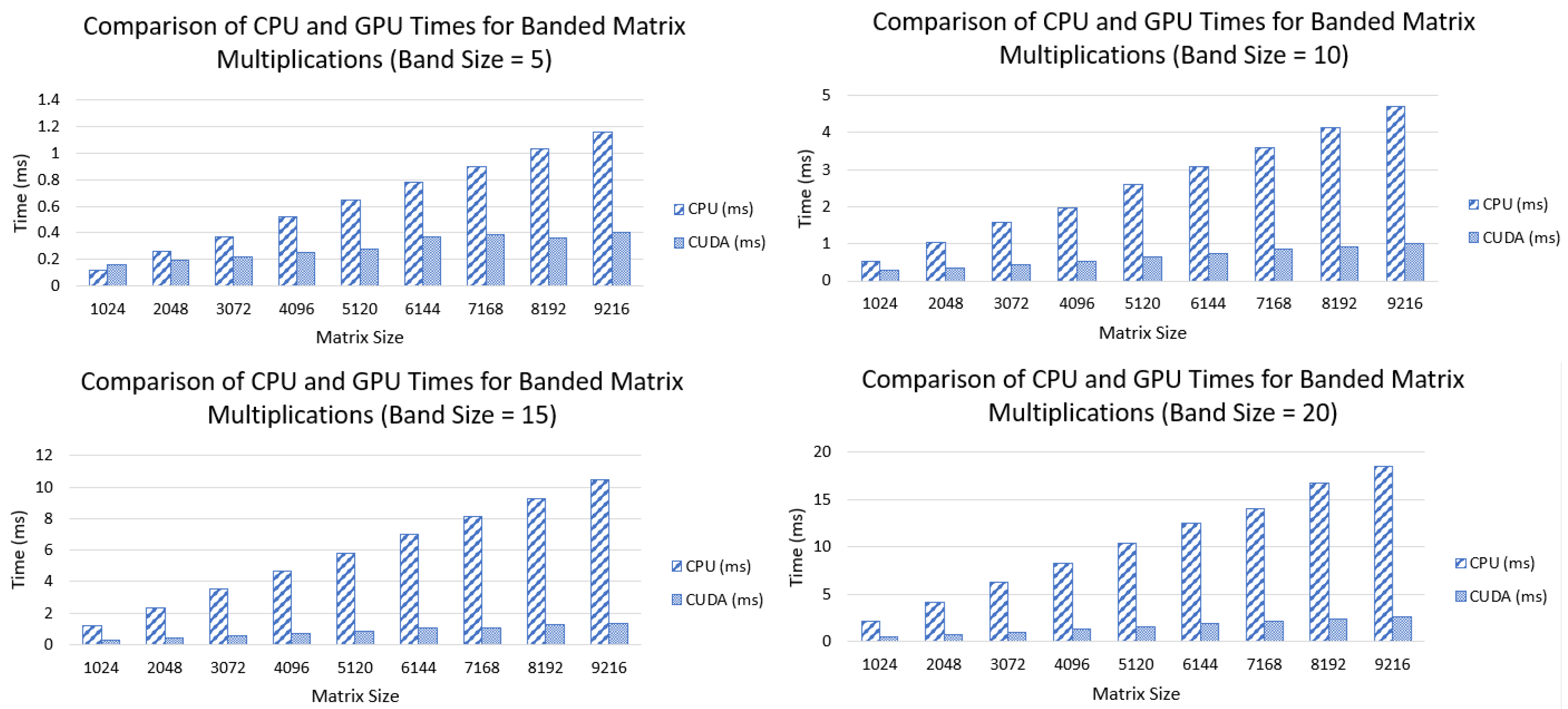
• Compare the performances of the proposed GPU algorithms with their CPU implementations.

The work presented in this paper is a significantly extended version of [22]. For ease of presentation, we borrow the central concepts of diagonal storage from [22].

The rest of the paper is organized in the following way. Section 2 presents a brief overview of the literature on the matrix multiplication problem in GPU architectures. Section 3 reviews the diagonal storage schemes HM  [20] and CDM [22], while general matrix multiplication with matrices stored in CDM is described in Section 4. With a short discussion on GPU architecture in Section 5, we provide a detailed description of the new GPU algorithms for banded and structured sparse matrix multiplication in Section 6. Section 7 presents the results of numerical experiments with the GPU algorithms. Finally, in Section 8, we give our concluding remarks.

2. Related Work

In the area of dense matrix multiplication, achieving high efficiency via GPU computing is well studied [9,23,24,25]. Early work [26] on dense matrix multiplication using GPUs framed the computation as a multitexture multiplication and blending operation. The user-programmable shared memory provided by subsequent GPU architectures enabled higher-performing data-parallel schemes via shared memory and registers [27,28]. The evolution of GPU math libraries employed more sophisticated code generation and kernel selection components to improve the performance of dense matrix multiplication. NVIDIA’s cuBLAS library provides an extended cublasGemmEx interface where carefully trained heuristics allow the caller to select from among 24 different dense matrix multiplication algorithms. For the purpose of optimization, it is common for cuBLAS to consider a wide range of data-parallel and fixed-split [29] variants implemented via these algorithms and assemble each variant into its own architecture-specific kernel program.

Unlike dense matrix multiplication, the implementation of sparse matrix multiplication in the current generic architectures is significantly more challenging. Among others, as identified by Matam et al. [30], variations in the nature of the sparsity introduce (i) load balancing problems among threads, (ii) optimization problems associated with irregular memory access patterns, and (iii) memory management problems due to the difficulties associated with the prediction of the output size. The authors also pointed out that GPU implementation poses further challenges in sparse matrix multiplication. In addition to the serious workaround required for the limited amount of shared memory available in GPU architecture, any divergence in the execution paths of a warp of threads against the single-program, multiple-data (SPMD) nature of GPU thread execution contributes to performance hindrance.

The GPU-based implementation of sparse matrix multiplication is available in CUSPARSE [31] and CUSP [32]. CUSP is termed an “expansion, sorting, and compression (ESC) method” due to the nature of its operation where it expands all values arising from scalar multiplication, sorts them, and finally compresses the entries with duplicate column indices. Consequently, the computational load is shifted to finding an efficient parallel sorting algorithm for the GPU (i.e., Radix-sort). This library routine stores the entire output on the GPU itself. Consequently, it only works on instances whose output size fits in the available global memory [33]). In addition, due to great variability in size, density, and structure, researchers [8] pointed out that it is reasonable to design special storage formats for matrices with certain characteristics to achieve better computational performance in the GPU.

3. Storage Schemes

In this section, we define the terminologies and notations used throughout the paper. Also, we discuss the storage schemes used in this work.

Let $A\in {\mathbb{R}}^{n\times n}$ be a banded matrix, where $k_l$ and $k_u$ are lower and upper bandwidths, respectively. Here, $a_{ij}=0$ if $i-j>k_l$ or $j-i>k_u$, where $a_{ij}$ refers to an element of matrix A and i, j denote the row index and column index of matrix A, respectively. Note that both indices i and j start with 0. Define $\overline{A_k}=\left\{a_{ij}|j-i=k\right\}$ and $\underline{A_k}=\left\{a_{ij}|i-j=k\right\}$ as the $k^{th}$ superdiagonal and $k^{th}$ subdiagonal of A, respectively.

Figure 2a displays a banded matrix where $k_u=2$ and $k_l=1$. Figure 2b displays the two-dimensional array representation used in BLAS (Basic Linear Algebra Subroutine), where ∗ represents a placeholder that is neither initialized nor referenced by any routine. The diagonals are placed in the following order: superdiagonals (i.e., $\overline{A_2}=[a_{02},a_{13}]$ and $\overline{A_1}=[a_{01},a_{12},a_{23}]$), main diagonal (i.e., $A_0$), and subdiagonals (i.e., $\underline{A1}=[a_{10},a_{21},a_{32}]$), preserving the column indexing. Figure 2c presents a variant of banded matrix storage by diagonals, where the nonexisting elements are pushed to the right such that the column indexing in the original matrix is not preserved.

Unless $k_l+k_u<<n$, the superfluous padding required along with the nonzero entities of super- and subdiagonals will outweigh the benefit of these compact storage schemes. Not only does the data structure become more complicated due to the additional storage needed for the nonexisting elements, but accessing the true matrix elements requires testing for sentinels, thereby fragmenting the control flow. This latter issue can become a significant performance bottleneck in contemporary many-core computer architectures.

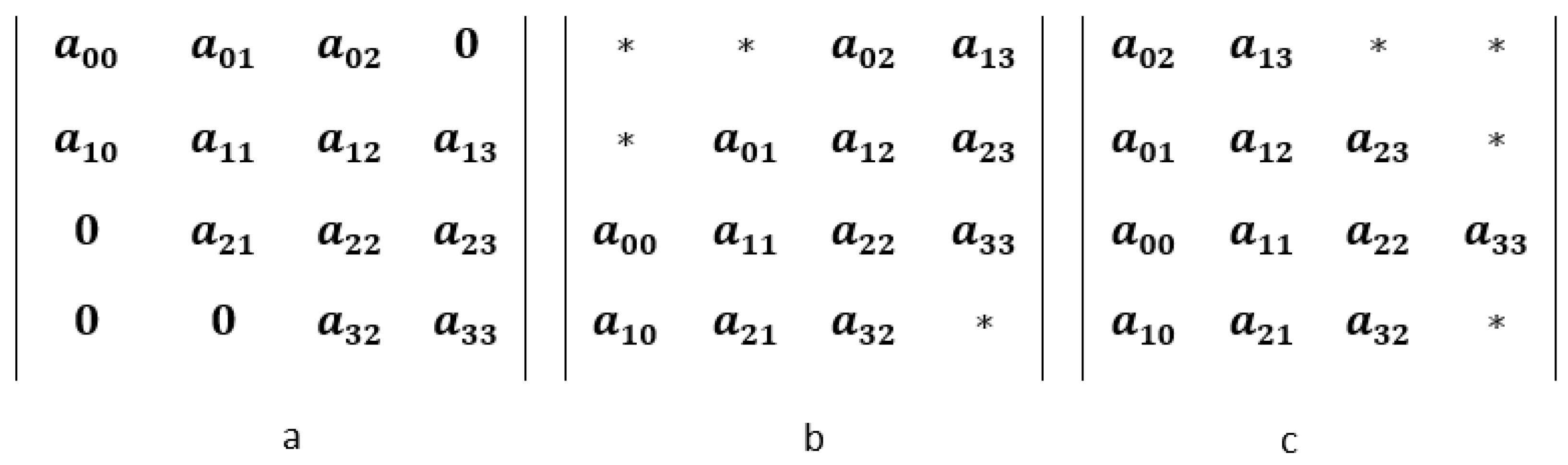
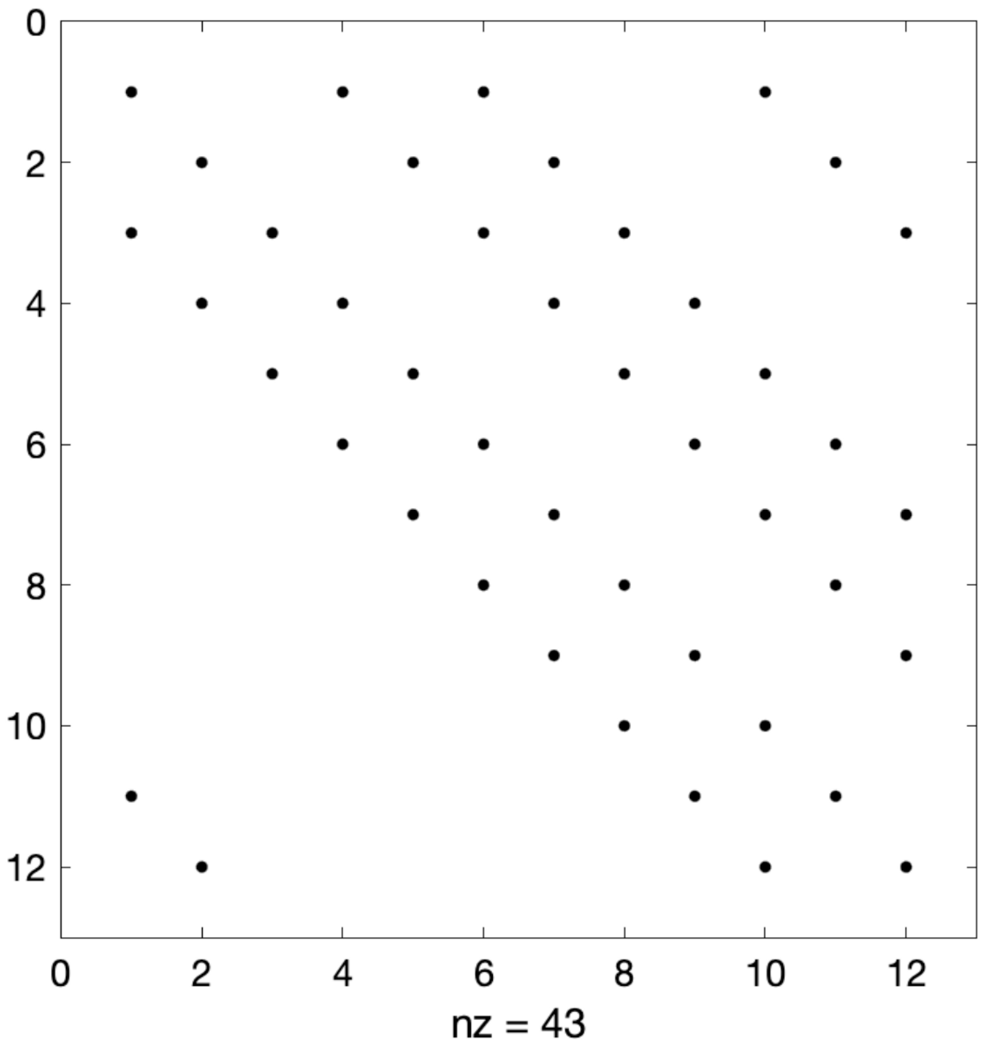
3.1. Diagonal Storage Scheme

The diagonal storage scheme proposed by Hossain and Mahmud [20] (called the HM scheme) for banded matrices is free from the aforementioned extraneous padded storage. It also supports a uniform representation of different kinds of structured matrices (e.g., diagonal, banded, triangular, symmetric, and fully dense matrices) and is independent of any orientation. In this section, we describe the diagonal storage scheme presented in [20]. From now on, we will use the terms “diagonal storage” and “HM” interchangeably to denote the storage scheme presented in [20].

For a dense matrix A, the HM diagonal storage scheme uses a one-dimensional array of size $n(k_u+k_l+1)-\frac{k_u(k_u+1)}{2}-\frac{k_l(k_l+1)}{2}.$ Note that, for a dense matrix A, $k_l=k_u=(n-1)$. Likewise, for an upper triangular matrix, we have $k_l=0$ and $k_u=n-1$, whereas for a lower triangular matrix, $k_u=0$ and $k_l=n-1$. The nonzero elements are ordered by diagonals as follows: $(A_0;\overline{A_1};\overline{A_2};\cdots \overline{A_{k_u}};\underline{A_1};\underline{A_2};\cdots \underline{A_{k_l}})$. For example, considering this storage scheme, the elements of the matrix in Figure 2a can be stored as

$$(a_{00},a_{11},a_{22},a_{33}|a_{01},a_{12},a_{23}|a_{02},a_{13}|a_{10},a_{21},a_{32})$$

where the symbol | is used to denote the boundary of the diagonals. According to the authors of [20], some elementary arithmetic calculations are required to access the elements of a specific diagonal in the HM scheme. For example, the index of the first element of the kth superdiagonal is calculated as $x+nk-\frac{k(k-1)}{2}$, where x is the starting index of the first element of the main diagonal $A_0$.

The indices of the diagonals that we follow in this paper are as follows. The index of the principle diagonal $A_0$ is 0. $\overline{A_i}$, a superdiagonal, and $\underline{A_j}$, a subdiagonal, are indexed as i and $-j$, respectively, where $i,j<n$.

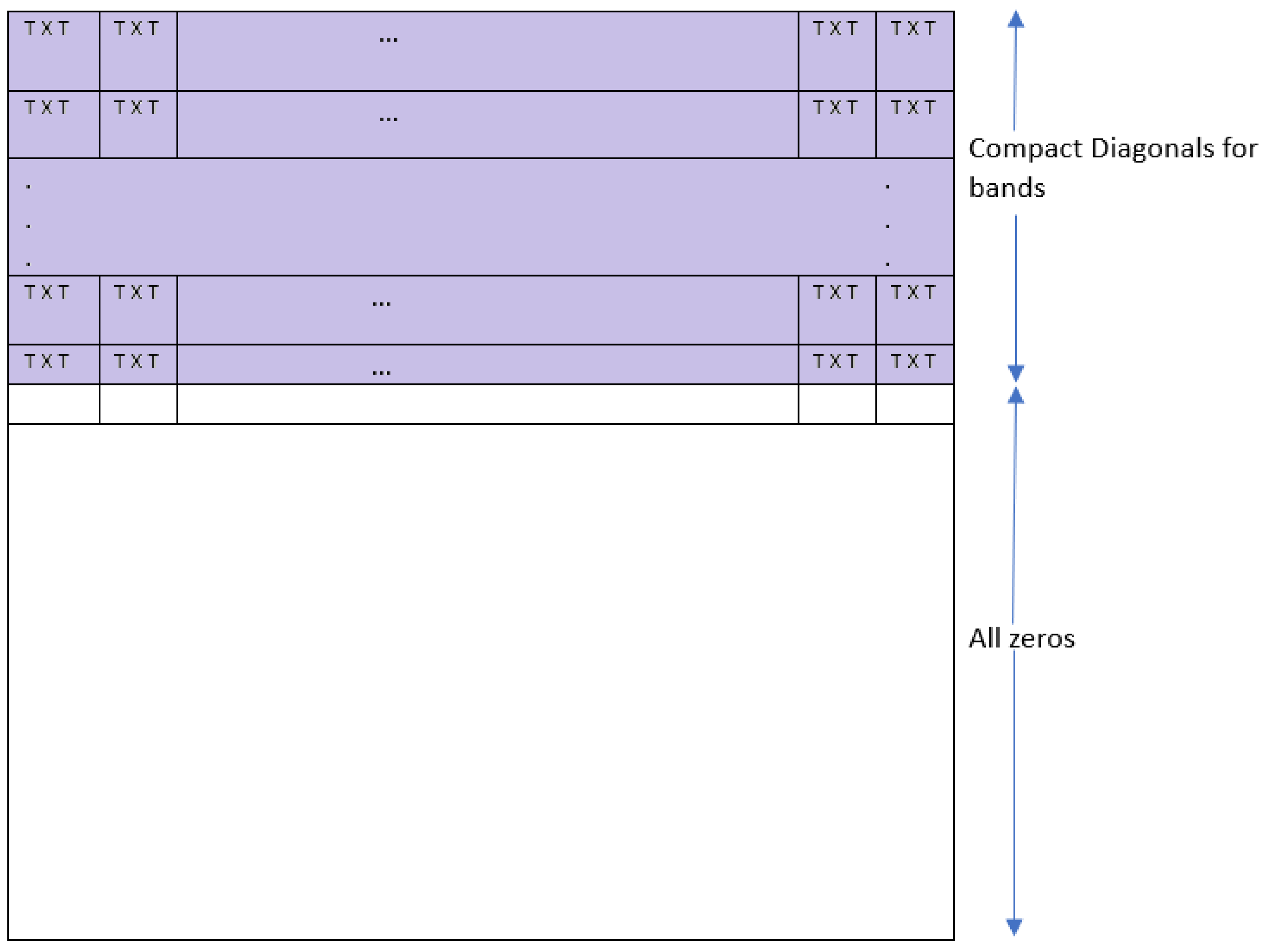
3.2. Compact Diagonal Storage Scheme

In this section, we will describe our proposed compact diagonal storage scheme. For the rest of the study, the two terms “Compact Diagonal” and “CDM” will be used interchangeably to denote our proposed storage scheme.

Rather than computing the super- and subdiagonals of the product $C=AB$ separately, we can pack compatible pairs of super- and subdiagonals in a vector of length n. The kth superdiagonal for $k=1,2,\dots ,n-1$ of matrix A is a vector $\overline{A_k}$ of length $n-k$,

$$\overline{A_k}=\left(\begin{array}{c}{a}_{0,k}\hfill \\ a_{1,k+1}\hfill \\ ⋮\hfill \\ a_{(n-k-1,n-1)}\hfill \end{array}\right).$$

Likewise, the kth subdiagonal is a vector $\underline{A_k}$ of length $n-k$,

$$\underline{A_k}=\left(\begin{array}{c}{a}_{k,0}\hfill \\ a_{k+1,1}\hfill \\ ⋮\hfill \\ a_{(n-1,n-k-1)}\hfill \end{array}\right).$$

We define the kth compact diagonal as

$$A_k=\left(\begin{array}{c}\overline{A_k}\hfill \\ \underline{A_{n-k}}\hfill \end{array}\right)$$

where the kth superdiagonal is stacked on top of the $(n-k)$th subdiagonal. In the case of dense matrices, we store each of these compact diagonals as a row of a matrix. For sparse matrices, all compact diagonals are kept in one long one-dimensional array, and we store some auxiliary arrays to represent the boundary between two diagonals.

It follows that each compact diagonal is a vector of length n. For example, the third compact diagonal (for $n=4$) is the vector $A_3$ of length 4:

$$A_3=\left(\begin{array}{c}\overline{A_3}\hfill \\ \underline{A_1}\hfill \end{array}\right)=\left(\begin{array}{c}{a}_{0,3}\hfill \\ a_{1,0}\hfill \\ a_{2,1}\hfill \\ a_{3,2}\hfill \end{array}\right)$$

where $\overline{A_3}$ is above the thick horizontal line and $\underline{A_1}$ is below it. The reverse of the kth compact diagonal is defined as

$$\widetilde{A_k}=\left(\begin{array}{c}\underline{A_k}\hfill \\ \overline{A_{n-k}}\hfill \end{array}\right)$$

by swapping the position of the superdiagonal and subdiagonal pair.

Figure 3 presents a visualization of a matrix of size $n=4$ (Figure 3a), the diagonal storage suggested in [20] (Figure 3b), and the compact diagonal storage (Figure 3c) proposed in the current study.

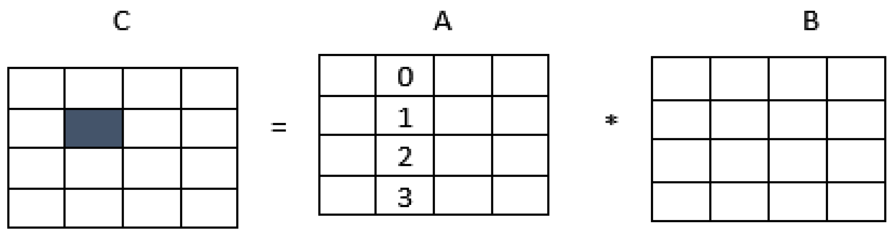
4. Compact Diagonal Matrix Multiplication

We are now ready to express the matrix multiplication operation

$$C\leftarrow C+AB$$

(1)

using compact diagonals. The main diagonal of the product matrix C is computed as

$$C_0=C_0+A_0{B}_0+\sum _{k=1}^{n-1}{A}_k\widetilde{B_k}$$

For $n=4$,

$$\begin{array}{ccc}{C}_0& =& C_0+A_0{B}_0+A_1\widetilde{B_1}+A_2\widetilde{B_2}+A_3\widetilde{B_3}\hfill \\ \left(\begin{array}{c}{c}_{0,0}\hfill \\ c_{1,1}\hfill \\ c_{2,2}\hfill \\ c_{3,3}\hfill \end{array}\right)& =& \left(\begin{array}{c}{c}_{0,0}\hfill \\ c_{1,1}\hfill \\ c_{2,2}\hfill \\ c_{3,3}\hfill \end{array}\right)\hfill \\ \\ & & +\left(\begin{array}{c}{a}_{0,0}\hfill \\ a_{1,1}\hfill \\ a_{2,2}\hfill \\ a_{3,3}\hfill \end{array}\right)\ast \left(\begin{array}{c}{b}_{0,0}\hfill \\ b_{1,1}\hfill \\ b_{2,2}\hfill \\ b_{3,3}\hfill \end{array}\right)+\left(\begin{array}{c}{a}_{0,1}\hfill \\ a_{1,2}\hfill \\ a_{2,3}\hfill \\ a_{3,0}\hfill \end{array}\right)\ast \left(\begin{array}{c}{b}_{1,0}\hfill \\ b_{2,1}\hfill \\ b_{3,2}\hfill \\ b_{0,3}\hfill \end{array}\right)\hfill \\ \\ & & +\left(\begin{array}{c}{a}_{0,2}\hfill \\ a_{1,3}\hfill \\ a_{2,0}\hfill \\ a_{3,1}\hfill \end{array}\right)\ast \left(\begin{array}{c}{b}_{2,0}\hfill \\ b_{3,1}\hfill \\ b_{0,2}\hfill \\ b_{1,3}\hfill \end{array}\right)+\left(\begin{array}{c}{a}_{0,3}\hfill \\ a_{1,0}\hfill \\ a_{2,1}\hfill \\ a_{3,2}\hfill \end{array}\right)\ast \left(\begin{array}{c}{b}_{3,0}\hfill \\ b_{0,1}\hfill \\ b_{1,2}\hfill \\ b_{2,3}\hfill \end{array}\right)\hfill \end{array}$$

The kth compact diagonal for $k=1,2,\dots ,n-1$ of the product matrix C is computed as

$$C_k=C_k+A_k{B_0}^{r_k}+\sum _{i=1}^{n-1}{A}_{(k+i)modn}{\widetilde{B_i}}^{r_k}$$

where the superscript $r_k$ indicates an upward shifting of the elements of vector $\widetilde{B_i}$ with wrap-around by k positions. To illustrate, consider

$$\widetilde{B_3}=\left(\begin{array}{c}{b}_{3,0}\hfill \\ b_{0,1}\hfill \\ b_{1,2}\hfill \\ b_{2,3}\hfill \end{array}\right).$$

For $k=1$, we have

$${\widetilde{B_3}}^{r_1}=\left(\begin{array}{c}{b}_{0,1}\hfill \\ b_{1,2}\hfill \\ b_{2,3}\hfill \\ b_{3,0}\hfill \end{array}\right).$$

Then, the first compact diagonal of the product matrix C is obtained as

$$\begin{array}{ccc}{C}_1& =& C_1+A_1{B}_0^{r_1}+A_2{\widetilde{B_1}}^{r_1}+A_3{\widetilde{B_2}}^{r_1}+A_0{\widetilde{B_3}}^{r_1}\hfill \\ \left(\begin{array}{c}{c}_{0,1}\hfill \\ c_{1,2}\hfill \\ c_{2,3}\hfill \\ c_{3,0}\hfill \end{array}\right)& =& \left(\begin{array}{c}{c}_{0,1}\hfill \\ c_{1,2}\hfill \\ c_{2,3}\hfill \\ c_{3,0}\hfill \end{array}\right)\hfill \\ \\ & & +\left(\begin{array}{c}{a}_{0,1}\hfill \\ a_{1,2}\hfill \\ a_{2,3}\hfill \\ a_{3,0}\hfill \end{array}\right)\ast \left(\begin{array}{c}{b}_{1,1}\hfill \\ b_{2,2}\hfill \\ b_{3,3}\hfill \\ b_{0,0}\hfill \end{array}\right)+\left(\begin{array}{c}{a}_{0,2}\hfill \\ a_{1,3}\hfill \\ a_{2,0}\hfill \\ a_{3,1}\hfill \end{array}\right)\ast \left(\begin{array}{c}{b}_{2,1}\hfill \\ b_{3,2}\hfill \\ b_{0,3}\hfill \\ b_{1,0}\hfill \end{array}\right)\hfill \\ \\ & & +\left(\begin{array}{c}{a}_{0,3}\hfill \\ a_{1,0}\hfill \\ a_{2,1}\hfill \\ a_{3,2}\hfill \end{array}\right)\ast \left(\begin{array}{c}{b}_{3,1}\hfill \\ b_{0,2}\hfill \\ b_{1,3}\hfill \\ b_{2,0}\hfill \end{array}\right)+\left(\begin{array}{c}{a}_{0,0}\hfill \\ a_{1,1}\hfill \\ a_{2,2}\hfill \\ a_{3,3}\hfill \end{array}\right)\ast \left(\begin{array}{c}{b}_{0,1}\hfill \\ b_{1,2}\hfill \\ b_{2,3}\hfill \\ b_{3,0}\hfill \end{array}\right).\hfill \end{array}$$

Matrix transposition is an algorithmic building block for algorithms such as Fast Fourier Transform (FFT) and K-means clustering [34]. The MKL implementation of BLAS provides transposed matrix multiplication,

$$C\leftarrow C+A^{\top }B,C\leftarrow C+A{B}^{\top },$$

as well as symmetric rank-k (SYRK) and rank-$2k$ (SYR2K) updates,

$$C\leftarrow A{A}^{\top }+C,C\leftarrow A{B}^{\top }+B{A}^{\top }+C$$

respectively. With traditional row-major (or column-major) storage, the naive in-place transposition incurs $\Omega \left(n^2\right)$ I/O operations. In a computer with multilevel hierarchical memory, this translates to $\Omega \left(n^2\right)$ cache misses, resulting in an unacceptably high penalty for performance. Both CDM and HM almost entirely avoid performance degradation due to transposed access to matrix elements. To see this, consider an arbitrary element $a_{i,j}$ of matrix A. Without loss of generality, assume that $i<j$ and that $k=(j-i)$. It follows that $a_{i,j}$ is stored in compact diagonal k which has the form

$$A_k=\left(\begin{array}{c}\overline{A_k}\hfill \\ \underline{A_{n-k}}\hfill \end{array}\right)$$

and that $a_{i,j}$ is an element of superdiagonal $\overline{A_k}$. Now, consider the reverse $\widetilde{A_k}$ of the kth compact diagonal

$$\widetilde{A_k}=\left(\begin{array}{c}\underline{A_k}\hfill \\ \overline{A_{n-k}}\hfill \end{array}\right)$$

Element $a_{i,j}$ of matrix A is located in row j and column i in the transposed matrix $B=A^{\top }$. We claim that $a_{i,j}$ is stored in the kth compact diagonal $B_k$ of matrix B and that $B_k=\widetilde{A_k}$. It is clear that in the transposed matrix we have $i>j$ so that $k=(i-j)$. By definition,

$$B_k=\left(\begin{array}{c}\overline{B_k}\hfill \\ \underline{B_{n-k}}\hfill \end{array}\right)=\left(\begin{array}{c}\underline{A_k}\hfill \\ \overline{A_{n-k}}\hfill \end{array}\right),$$

thereby establishing that transposed access with diagonal storage is obtained without any data movement.

Basic linear algebra operations with compact diagonals (CDM) can be viewed as a specialization of HM [20] in that common types of square structured matrices such as symmetric, triangular, banded, and Hessenberg matrices can be treated in a uniform way using HM.

One final note about the actual computer implementation of matrix operations with HM or CDM is concerned with the apparent matrix nonzeros being shuffled around in the diagonal or compact diagonal vectors $A_k=\left(\begin{array}{c}\overline{A_k}\hfill \\ \underline{A_{n-k}}\hfill \end{array}\right)$, $\widetilde{A_k}=\left(\begin{array}{c}\underline{A_k}\hfill \\ \overline{A_{n-k}}\hfill \end{array}\right)$, and ${\widetilde{B_i}}^{r_k}$. However, it is not difficult to see that access to the relevant nonzero elements of diagonal vectors during iterative computation can be provided through the loop variables so that once the diagonals are laid out as vectors, no further data movement is needed in their access.

5. GPU Programming

Owing to their high performance-to-price and performance-to-energy ratios, graphics processing units (GPUs) have been increasingly used in recent years on a broad range of computationally demanding and complex problems. These programmable parallel processors are designed to achieve higher throughput with computing power exceeding multicore CPUs by deploying thousands of relatively light-weight compute threads in parallel [35]. NVIDIA’s GPU with the CUDA (Compute Unified Device Architecture) environment supports a standard high-level language (i.e., C language) interface to manipulate the compute cores. It also supports the models of computations that explicitly combine both task-based parallelism and data-based parallelism [36].

The code running on the GPU is traditionally called the kernel. CUDA threads are grouped into thread blocks. Threads in a thread block reside on the same streaming multiprocessor (SM) of a GPU that can share data using shared memory and synchronize. Each thread in a thread block has a unique identification number. Each group of 32 consecutive threads from the same thread block is called a warp. It is the primary unit of execution in an SM. Each SM contains a warp scheduler that is responsible for scheduling the warps to the underlying cores on the SM.

6. Algorithms

6.1. Banded Matrix–Matrix Multiplication

We implemented banded matrix–matrix multiplication using the CDM data structure. Banded matrices that arise in real-life applications usually have narrow bands compared to their dimensions [37], which means that the CDM representation of the nonzero diagonals of narrow banded matrices are packed with only a small number of zeros. Thus, the compact diagonal scheme is more suitable for this case. On the other hand, we implemented structured sparse matrix–matrix multiplication using the HM data structure, which is described in the next section. As a banded matrix is a special kind of structured sparse matrix, the implementation that we are going to describe in the next subsection can also be used for banded matrix–matrix multiplication. In the case that the width of a banded matrix is large with respect to n, the number of zeros for padding increases, so the HM data structure is more suitable than CDM.

In our GPU algorithm, a thread will compute one entry of matrix C. As matrix C is also a banded matrix, it is natural to assign a 2-D thread block of size $T\times T$ to compute $T^2$ entries of C. So, the total number of threads in a thread block is $T^2$, which should be a multiple of warp size. We choose $T=2^d$, where $d=4$.

Before describing GPU multiplication in greater detail, we first provide a high-level overview of the overall algorithm.

Figure 4 displays the logical mapping of GPU threads to the computed entries of the product matrix C. A row corresponds to a compact diagonal of matrix C, while the entries of matrix C are computed in blocks (tiles) as shown. Suppose the elements in the highlighted tile of the C matrix of Figure 5 are to be computed using the corresponding thread block. The tiles marked $0,1,2,3$ from matrix A are needed to compute the elements in the highlighted tile of C. The GPU algorithm works in a block-iterative manner. In the i-th block iteration, where $0\le i<4$, of Figure 5, a thread block brings the i-th tile of matrix A to the shared memory, performs all required multiplications between the tile elements from A and the nonzeros from B, such that the multiplications contribute to the elements in the highlighted tile of matrix C. The algorithm terminates once all the tiles of matrix Cb are computed.

A banded matrix X is represented by the following two lists and one integer. Here, a diagonal of X will be stored as a row in the CDM data structure. As all the diagonals in X are centered around the principal diagonal, in the CDM storage scheme, the (short) diagonal of zeros can be appended either at the beginning or at the end of the nonzero diagonals.

• Integer $dgX$ representing the number of compact diagonals in X.
• List of integers $DsX$ of length $dgX$, which is the list of the indices of the diagonals of X.
• $Xlist$: One-dimensional list of length $dgX\times n$ containing the values of X.

We use $nzX$ to denote the number of nonzeros in matrix X.

Given two banded matrices A and B, matrix C will also be a banded matrix whose compact diagonals are computed via the following formula. Compact diagonal i of C is computed by multiplying the k-th compact diagonal of A and the $(i-k)$-th compact diagonal of B, where $0\le k<n$ and $(i-k)$ are computed as moduli of n. That the indices of the compact diagonals of C can be computed before numerically computing the product $AB$ enables us to preallocate memory for product matrix C.

As depicted in Figure 5, threads in a 2-D thread block of size $T\times T$ know the identity of the elements of the block of C, in the CDM representation, that they are computing. The band size of C may or may not be divisible by T. Consequently, some threads from the thread blocks that are computing the compact diagonals near the bottom edge in Figure 5 may remain idle. In an outer (i.e., block) iteration, each thread block uses shared memory to bring a block of entries of the same size ($T\times T$) (that can contribute to compute the assigned block of C) and store it in the shared memory. Then, the algorithm uses a thread block synchronization to make sure all threads can complete their computational contributions.

The shared memory will be filled with entries from A in blocks (of size $T\times T$) from top to bottom, as shown in Figure 4. As each thread is computing one entry of C, the number of possible multiplications that contribute toward that entry and involve entries from A in the shared memory is T. So, during each iteration, each thread will perform T multiplications. The entries from B are accessed via the global memory. For each multiplication, a thread needs to know the indices of the diagonals of the entries from both A and C. So, it also needs to know the index of the diagonal of the entry from matrix B. To accelerate this process, we store the starting index of each diagonal in $Blist$ in a dense format. We pass this information as a separate array called $BdiagDense$ to our algorithm. The algorithm is given in Algorithm 1.

Algorithm 1:CUDA Algorithm for Banded Matrix–Matrix Multiplication

We observe that for a thread block, in one iteration, in general, all threads access the shared memory T times. That means that each entry of A will be used T times. This gives us an advantage in terms of the “data reuse” of shared memory. The number of entries from B that need to be accessed for these multiplications is more than $T^2$. But, to know the exact number, we need to specify the diagonal indices from both A and B.

During an iteration of the algorithm, to compute an entry from block $C[i_1\cdots i_2][j_1\cdots j_2]$ of C, where $i_2-i_1=j_2-j_1=T$, we bring a block of size $T\times T$ from A (denoted by $A[k_1\cdots k_2][j_1\cdots j_2]$, $k_2-k_1=T$) into the shared memory. So, the indices of the diagonals of matrix B from which the other entries come are in the set $\{i_1-k_2\dots i_2-k_1\}$. For simplicity, we assume that all diagonals whose indices are given in the set exist in B. From the above information, we can compute the number of entries of matrix B which need to be accessed to perform $T^3$ multiplications.

Unlike the entries of A, we do not bring the entries of B into the shared memory during multiplication to avoid high memory traffic. To see this, assume the entries from matrix B are to be brought into the shared memory for $T^3$ multiplications. As the total number of diagonals in B required in any iteration for a thread block is $2T-1$ and the maximum number of entries in any of those diagonals is $2T-1$, it is a good idea to bring a block of size $(2T-1)\times (2T-1)\approx 4T^2$ of B into the shared memory to avoid code divergence in performing these $T^3$ multiplications. So, the average number of times an entry of B will be reused (if brought into shared memory) is $T/4$. As T is small (ranging from 4 to 16), $T/4$ is also small. This observation is true for dense matrix multiplications, where the matrices are stored in the CDM storage scheme.

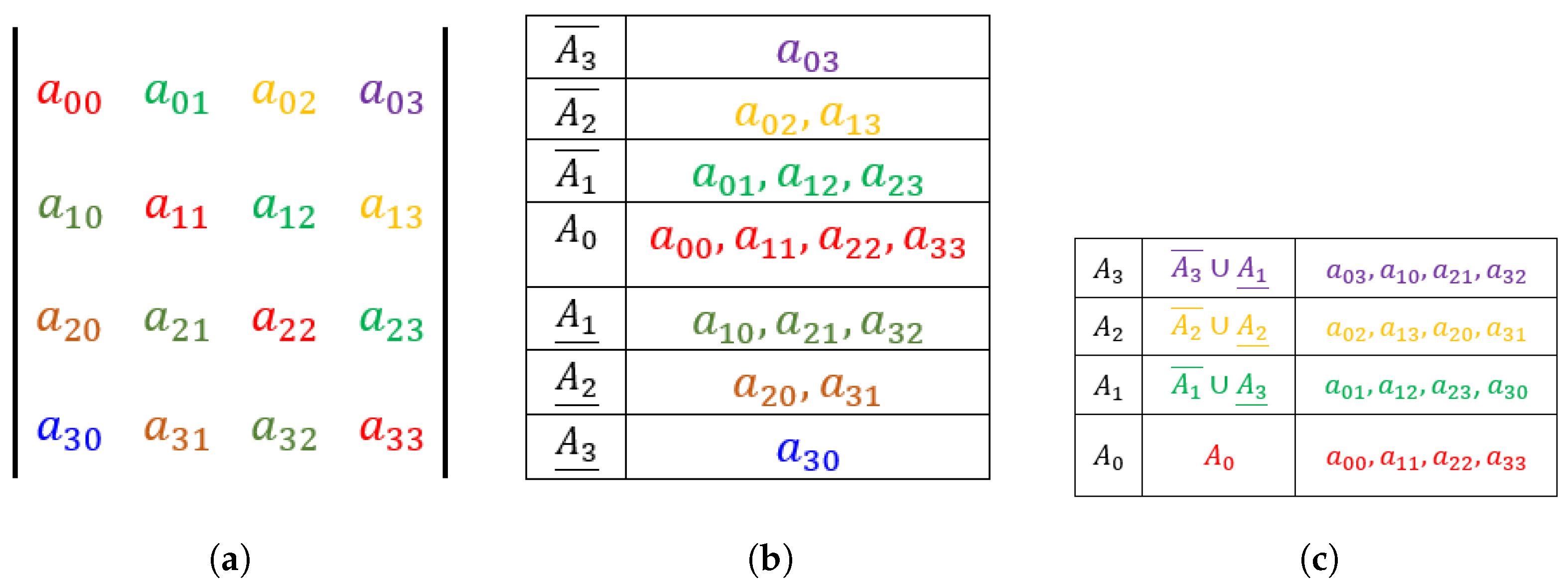
6.2. Structured Sparse Matrix–Matrix Multiplication

We consider two main techniques for designing a structured sparse matrix–matrix parallel multiplication algorithm targeting GPU architecture: (i) each entry of C is computed using one thread, and (ii) all multiplications that are associated with an entry of either A or B are performed using one thread.

Both of the above approaches have a similar outlook from a data locality point of view. That is, we expect that multiple threads in a warp are accessing entries from matrices A, B, or C that are physically stored closely in the global memory. The first approach is a pure parallel approach. The second approach requires atomic operations since two different threads might contribute to the same entry of C at the same time. In this work, we implement this second approach and claim that the second approach minimizes computational overhead.

Let i and j be two diagonal indices of matrices A and B, respectively, where $-n<i,j<n$. The multiplications between the elements of the i-th diagonal of A with the elements of the j-th diagonal of B will contribute to the $(i+j)$-th diagonal of C, where $-n<(i+j)<n$. From this observation, we can expect that C is potentially more dense compared to A or B.

The number of multiplications required to compute an entry of C varies widely due to the irregular distribution of nonzero diagonals in matrices A and B. In the first approach, such disproportionate thread workload creates code divergence in thread blocks, affecting the performance negatively. Moreover, a thread that is assigned to compute an entry from C needs to examine every possible pair of diagonals from A and B. If a pair of diagonals from A and B exist (i.e., nonzero), then a multiplication is performed and the associated entry of matrix C is updated. As both A and B are sparse, there will be fewer nonzero diagonal pairs compared to the quadratic search space, thereby increasing the overhead.

In the second approach, a thread is assigned to perform all multiplications associated with one entry from one of the operands A or B. Without loss of generality, let A be the selected operand. The number of threads required to compute the matrix product $C=AB$ is equal to the number of nonzeros in matrix A (i.e., $nzA$). A thread first computes the index of the entry from each nonzero diagonal in B with which the entry from A will be multiplied. After multiplication, the thread also updates the corresponding entry in C via an atomic operation. In this approach, we expect to experience less code divergence than that of the first approach.

In summary, we conclude that although both approaches have similar data locality challenges and disadvantages, we prefer the second approach due to its favorable (expected) code divergence compared with the first approach.

A structured sparse matrix (say, X) is represented by the following three lists and one integer value. Here, a diagonal of X will be treated as a diagonal in the HM data structure.

• An integer value $dgX$ that represents the number of HM diagonals in X. In structured sparse matrices, we know that only some of the diagonals have nonzeros. We will store those diagonals only.
• A list of integers $DsX$ (of length $dgX$) that stores the indices of the diagonals of X. The first element of this array is 0 if the principal diagonal is dense. It stores the indices of the super diagonals first, followed by those of the subdiagonals. For superdiagonal indices, those are stored in ascending order. For subdiagonal indices, those are stored in descending order.
• $Xlist$: This is a one-dimensional array that stores the entries of X. The entries from the same diagonal are kept together according to their column indices.
• A list of integers $StartDgX$ (of length $dgX$) that stores the indices of the entries in $Xlist$ for each diagonal of X.

We use $nzX$ to present the number of nonzeros in sparse matrix X.

A thread that handles all multiplications associated with an entry from A will run in a loop for each diagonal of B. An entry from A can be from a super-, sub-, or principal diagonal of A. In the same way, a diagonal from B can also be a super-, sub-, or principal diagonal of B. We enumerate thirteen different cases based on the different choices of the diagonals of A and B. These thirteen different cases are grouped into three categories. In each of the thirteen cases, given an entry from A and a diagonal from B, our objective is to find the entry in the diagonal of B that can be multiplied with the entry of A. After a multiplication, the thread will find the entry in C to which this multiplication will contribute. In our descriptions of the thirteen cases below, we will use three index variables $i,j,k$, where $n>i,j,k\ge 0$. For an entry of A, it is possible that there might be no entry from a particular diagonal of B with which it can be multiplied. In short, we describe the situation by saying that such an entry in B does not exist.

In the first category of cases, we describe the cases that can arise while computing the principal diagonal of C.

• The multiplications between the principal diagonals of A and B contribute to the principal diagonal of C. Each multiplication can be described in the following way, with the left index 0 indicating the (principal) diagonal:

  $$C\left[0\right]\left[i\right]=A\left[0\right]\left[i\right]\ast B\left[0\right]\left[i\right].$$
• The entries of A and B are from the i-th superdiagonal and $(-i)$-th subdiagonal, respectively. Each of the multiplications can be described in the following way: $C\left[0\right]\left[j\right]=A\left[i\right]\left[j\right]\ast B[-i]\left[j\right]$.
• The entries of A and B are from the $(-i)$-th subdiagonal and i-th superdiagonal, respectively. Each of the multiplications can be described in the following way: $C\left[0\right][i+j]=A[-i]\left[j\right]\ast B\left[i\right]\left[j\right]$.

In the second category, we have five different cases that arise while computing the entries in the superdiagonals of C.

• Let $A\left[i\right]\left[k\right]$ and j be an entry from A and an index of a diagonal from B, respectively. If $B\left[j\right][i+k]$ exists, then $B\left[j\right][i+k]$ will be multiplied with $A\left[i\right]\left[k\right]$, and this multiplication will contribute to $C[i+j]\left[k\right]$.
• Let $A\left[0\right]\left[i\right]$ and j be an entry from the principle diagonal of A and an index of a diagonal from B, respectively. $A\left[0\right]\left[i\right]$ will be multiplied with $B\left[j\right]\left[i\right]$ (if it exists), and their multiplication will contribute to $C\left[j\right]\left[i\right]$.
• Let $A\left[i\right]\left[j\right]$ be an entry from A. It can be multiplied with $B\left[0\right][i+j]$ (if it exists), and the multiplication result will contribute to $C\left[i\right]\left[j\right]$.
• Let $A\left[i\right]\left[k\right]$ and $-j$ be an entry from A and an index of a diagonal from B, respectively. Assume $i>j$ and $B[-j][i+k-j]$ exist. Then, $B[-j][i+k-j]$ will be multiplied with $A\left[i\right]\left[k\right]$, and the multiplication result will contribute to $C[i-j]\left[k\right]$.
• Let $A[-i]\left[k\right]$ and j be an entry from A and an index of a diagonal from B, respectively. Here, $j>i$. If $B\left[j\right]\left[k\right]$ exists, then $B\left[j\right]\left[k\right]$ will be multiplied with $A[-i]\left[k\right]$, and the multiplication result will contribute to $C[j-i][k+i]$.

In the third category, we have five different cases that arise while computing the entries in the subdiagonals of C. These five cases are obtained from the second category by switching the super- and subdiagonals of matrices.

All of the above thirteen cases can be obtained from the following two rules.

• Rule for matrix multiplication with coordinate matrix data structure: Let $A_c$ and $B_c$ be two matrices of size $n\times n$ stored in a coordinate storage scheme. We want to compute $C_c=A_c\times B_c$. An element $A_c\left[i\right]\left[j\right]$ will be multiplied with $B_c\left[j\right]\left[k\right]$, where $n>i,j,k\ge 0$, and $A_c\left[i\right]\left[j\right]\times C_c\left[j\right]\left[k\right]$ will contribute to $C_c\left[i\right]\left[k\right]$.
• Assume that we convert $A_c$ to matrix A stored in an HM structure. Let $A_c\left[i\right]\left[j\right]$ be an entry in $A_c$. This element will be $A[j-i]\left[min\right(i,j\left)\right]$ in the HM storage scheme.

As an example, let $A_c\left[i\right]\left[j\right]$ and $B_c\left[j\right]\left[k\right]$ be two elements of $A_c$ and $B_c$, respectively, in the coordinate scheme. Their multiplication will contribute to $C_c\left[i\right]\left[k\right]$ (also in the coordinate storage scheme). Without loss of generality, let $i<j<k$. Clearly, $A[j-i]\left[i\right]$, $B[k-j]\left[j\right]$, and $C[k-i]\left[i\right]$ are the corresponding elements of $A_c\left[i\right]\left[j\right],B_c\left[j\right]\left[k\right]$, and $C_c\left[i\right]\left[k\right]$ in the HM storage scheme, respectively. This is an example where two superdiagonal elements (from A and B) contribute to a superdiagonal of C (second category case 1). In the same way, by changing the inequality among $i,j$, and k, we can verify the rest of the 12 cases.

Algorithm 2 has a number of nested if⋯else blocks, which in practice can increase the code divergence among threads in the same thread block. In the worst case, this code divergence might significantly affect performance. One effective solution to overcome this code divergence issue is to have a few threads (for example, k, where $1<k\le 13$) per nonzero entry of A that will take care of all multiplications associated with that nonzero entry of A. The if⋯else part of the code can be restructured such that each of the if(condition){⋯}s will be mapped to one of the k threads exclusively. As all threads in a thread block will take care of the same if(condition){⋯}, we expect to have lower code divergence.

Algorithm 2:CUDA Algorithm for Structured Sparse Matrix–Matrix Multiplication

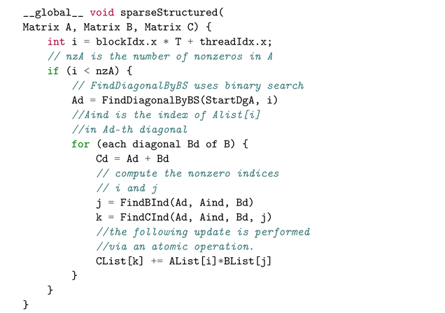
7. Experimental Results

In this section, we examine the performance of our GPU algorithms for matrix multiplication where the matrices are stored using the HM and CDM schemes. We conducted all of our experiments on a desktop computer that has an Intel i7-7700K processor (4.20 GHz) with four cores and 16 GB of RAM. Its L1, L2, and L3 cache sizes are 256 KB, 1.0 MB, and 8.0 MB, respectively. The GPU card that we used for our CUDA code execution is NVIDIA TITAN XP with 12 GB of memory of type GDDR 5X.

The computational study is divided into two parts. The first part is concerned with experimentation with banded matrices, and in the second part, we experiment with structured sparse matrices. The sparsity patterns (i.e., nonzero diagonals) are randomly generated. The calculations are performed in double precision.

7.1. Banded Matrix Multiplication

We employed nine different problem dimensions $n=$ 1024, 2048, 3072, 4096, 5120, 6144, 7168, 8192, 9216 with four different bandwidths $5,10,15,20$. Figure 6 displays the running times of sequential (CPU) and parallel (GPU) implementations. It is clear that the GPU implementation yields significant acceleration over the sequential version, giving the highest acceleration factor with the largest matrix dimension. More importantly, the rate of improvement scales nicely with the band size and matrix dimension. To investigate the scaling further, we conduct separate experiments with a fixed matrix dimension while varying the band size. The comparative running times of the experiment are displayed in Figure 7. The GPU speedup obtained vs. CPU, order of improvement, is quite evident and scales well with the increasing band size.

7.2. Structured Sparse Matrix Multiplication

In this section, we evaluate GPU matrix–matrix multiplication algorithms for structured sparse matrices, i.e., matrices where the nonzero diagonals are arbitrarily distributed instead of being confined within a narrow band around the main diagonal. In other words, the class of banded matrices can be considered as a special case of the class of structured sparse matrices. Numerical methods for solving partial differential equations using finite-difference discretization give rise to linear systems where the coefficient matrices display structured sparsity patterns. Standard banded matrix storage schemes including the one specified using BLAS are not directly applicable to structured sparse matrices. Consequently, structured sparse matrices can be treated as general sparse matrices and be stored, for example, in a compressed sparse row (CRS) requiring auxiliary data structures. Thus, the class of structured sparse matrices presents an interesting case study on its own.

In

Table 1. Comparison of computational times for computing structured sparse matrix multiplication between CPU and GPU.

Matrix	dgA,	dgB,	nzC	CPU	CUDA	Time
Size	nzA	nzB		(ms)	(ms)	Ratio
1000	9, 7446	5, 3968	33,824	4.33	0.16	27
2000	9, 15,003	15, 25,201	203,935	2.12	0.21	10
3000	29, 75,336	15, 39,207	990,791	11.66	0.39	30
4000	29, 97,958	35, 120,652	2,816,485	38.60	0.88	44
5000	59, 256,918	35, 150,005	6,625,325	99.52	1.89	52
6000	89, 473,743	75, 381,842	17,999,054	440.61	6.78	65
7000	99, 615,376	75, 451,559	23,585,358	560.69	8.92	63
8000	109, 767,508	35, 247,865	18,893,371	307.67	5.26	5 8
9000	59, 470,354	75, 593,612	24,161,386	444.00	7.09	63
10,000	109, 938,979	35, 310,455	24,738,090	365.51	6.34	58

and

Table 2. Comparison of computational times for computing structured sparse matrix multiplications of dimension 10,000 between CPU and GPU by varying their diagonal numbers.

dgA, nzA	dgB, nzB	nzC	CPU	CUDA	Time
			(ms)	(ms)	Ratio
200, 1,746,454	200, 1,734,514	69,689,071	4812.40	66.62	72
300, 2,574,174	300, 2,599,683	76,317,794	11,031.72	141.86	78
400, 3,462,833	200, 3,499,657	75,463,181	19,733.96	241.23	82
500, 4,358,737	500, 4,372,825	75,504,513	31,817.91	358.39	89
600, 5,237,042	600, 5,233,209	75,281,188	46,549.84	468.83	99

, we present the running time of CPU and GPU structured sparse matrix multiplication experiments. The nonzero diagonals are randomly picked for the argument matrices A and B. We include the number of diagonals (dgA, dgB) as well as the total number of nonzeros (nzA, nzB) for arguments A and B, respectively. It is to be emphasized that the product C need not have a structured sparse form. In fact, C may contain partially filled (with nonzeros) diagonals. In Table 1, we vary both matrix size and number of diagonals in the generated test matrices A and B. The running times for the CPU and GPU implementations exhibit relative performance profiles similar to that for banded matrices. The running time performance of CPU and GPU improves with the matrix size and the number of diagonals because of the increase in the computational work and the improved data locality. Moreover, the relative performance (the ratio of CPU and GPU running time) shows good scalability, yielding a speedup of 65 times. In Table 2, the matrix dimension is held constant at 10,000 × 10,000, while the number of nonzero diagonals in matrices A and B are increased from 200 to 600. In this case, the GPU algorithm exhibits a better performance gain, yielding a top speedup of 100 times.

8. Summary and Concluding Remarks

In this paper, we have explored a diagonally structured storage scheme, the CDM, where pairs of compatible superdiagonals and subdiagonals are packed together in vectors of uniform length. This compact scheme avoids storing and computing with short vectors (diagonals). As its predecessor, the diagonal storage scheme, the CDM provides orientation (row/column)-independent stride-1 access to matrix elements and enables vector arithmetic wherever the underlying CPU architecture admits. We have presented, for the first time, GPU algorithms to perform matrix multiplication using the recently proposed diagonal storage schemes HM and CDM. An extensive set of numerical experiments with banded and structured sparse matrices convincingly established the advantage of our diagonally structured storage mechanism in implementing matrix–matrix multiplication, a computational workhorse in scientific computation. The experiments clearly demonstrate that the implemented GPU algorithms are highly scalable and give significant parallel speedups, up to two orders of magnitude.

The storage scheme based on matrix diagonals, as opposed to rows/columns, provides an alternative approach to implementing linear algebraic kernel operations in the BLAS specification. More specifically, this new storage scheme avoids explicit matrix transposition and thereby has the potential to improve the performance of BLAS level-2 and level-3 operations. We are currently developing sequential, multicore, and many-core parallel algorithms for general sparse matrix multiplication.

References

1. Abdullah, W.M.; Awosoga, D.; Hossain, S. Efficient Calculation of Triangle Centrality in Big Data Networks. In Proceedings of the 2022 IEEE High Performance Extreme Computing Conference (HPEC), Waltham, MA, USA, 19–23 September 2022; pp. 1–7. [Google Scholar] [CrossRef]
2. Gao, J.; Ji, W.; Chang, F.; Han, S.; Wei, B.; Liu, Z.; Wang, Y. A systematic survey of general sparse matrix-matrix multiplication. ACM Comput. Surv. 2023, 55, 1–36. [Google Scholar] [CrossRef]
3. Kepner, J.; Gilbert, J. Graph Algorithms in the Language of Linear Algebra; SIAM: Philadelphia, PA, USA, 2011. [Google Scholar]
4. Kepner, J.; Jananthan, H. Mathematics of Big Data: Spreadsheets, Databases, Matrices, and Graphs; MIT Press: Cambridge, MA, USA, 2018. [Google Scholar]
5. Shen, L.; Dong, Y.; Fang, B.; Shi, J.; Wang, X.; Pan, S.; Shi, R. ABNN2: Secure two-party arbitrary-bitwidth quantized neural network predictions. In Proceedings of the 59th ACM/IEEE Design Automation Conference, San Francisco, CA, USA, 10–14 July 2022; pp. 361–366. [Google Scholar]
6. Gholami, A.; Kim, S.; Dong, Z.; Yao, Z.; Mahoney, M.W.; Keutzer, K. A survey of quantization methods for efficient neural network inference. In Low-Power Computer Vision; Chapman and Hall/CRC: Boca Raton, FL, USA, 2022; pp. 291–326. [Google Scholar]
7. Gundersen, G. The Use of Java Arrays in Matrix Computation. Master’s Thesis, University of Bergen, Bergen, Norway, 2002. [Google Scholar]
8. Yang, W.; Li, K.; Liu, Y.; Shi, L.; Wan, L. Optimization of quasi-diagonal matrix–vector multiplication on GPU. Int. J. High Perform. Comput. Appl. 2014, 28, 183–195. [Google Scholar] [CrossRef]
9. Benner, P.; Dufrechou, E.; Ezzatti, P.; Igounet, P.; Quintana-Ortí, E.S.; Remón, A. Accelerating band linear algebra operations on GPUs with application in model reduction. In Proceedings of the Computational Science and Its Applications–ICCSA 2014: 14th International Conference, Guimarães, Portugal, 30 June–3 July 2014; Proceedings, Part VI 14. Springer: Cham, Switzerland, 2014; pp. 386–400. [Google Scholar]
10. Dufrechou, E.; Ezzatti, P.; Quintana-Ortí, E.S.; Remón, A. Efficient symmetric band matrix-matrix multiplication on GPUs. In Proceedings of the Latin American High Performance Computing Conference, Valparaiso, Chile, 20–22 October 2014; Springer: Berlin/Heidelberg, Germany, 2014; pp. 1–12. [Google Scholar]
11. Madsen, N.K.; Rodrigue, G.H.; Karush, J.I. Matrix multiplication by diagonals on a vector/parallel processor. Inf. Process. Lett. 1976, 5, 41–45. [Google Scholar] [CrossRef]
12. Tsao, A.; Turnbull, T. A Comparison of Algorithms for Banded Matrix Multiplication; Citeseer: Vicksburg, MS, USA, 1993. [Google Scholar]
13. Vooturi, D.T.; Kothapalli, K.; Bhalla, U.S. Parallelizing Hines matrix solver in neuron simulations on GPU. In Proceedings of the 2017 IEEE 24th International Conference on High Performance Computing (HiPC), Jaipur, India, 18–21 December 2017; IEEE: Piscataway, NJ, USA, 2017; pp. 388–397. [Google Scholar]
14. Benner, P.; Dufrechou, E.; Ezzatti, P.; Quintana-Ortí, E.S.; Remón, A. Unleashing GPU acceleration for symmetric band linear algebra kernels and model reduction. Clust. Comput. 2015, 18, 1351–1362. [Google Scholar] [CrossRef]
15. Kirk, D.B.; Wen-Mei, W.H. Programming Massively Parallel Processors: A Hands-On Approach; Morgan Kaufmann: Burlington, MA, USA, 2016. [Google Scholar]
16. Munshi, A.; Gaster, B.; Mattson, T.G.; Ginsburg, D. OpenCL Programming Guide; Pearson Education: London, UK, 2011. [Google Scholar]
17. Volkov, V.; Demmel, J.W. Benchmarking GPUs to tune dense linear algebra. In Proceedings of the SC’08: Proceedings of the 2008 ACM/IEEE conference on Supercomputing, Austin, TX, USA, 15–21 November 2008; IEEE: Piscataway, NJ, USA, 2008; pp. 1–11. [Google Scholar]
18. Kurzak, J.; Tomov, S.; Dongarra, J. Autotuning GEMM kernels for the Fermi GPU. IEEE Trans. Parallel Distrib. Syst. 2012, 23, 2045–2057. [Google Scholar] [CrossRef]
19. Ortega, G.; Vázquez, F.; García, I.; Garzón, E.M. Fastspmm: An efficient library for sparse matrix matrix product on gpus. Comput. J. 2014, 57, 968–979. [Google Scholar] [CrossRef]
20. Hossain, S.; Mahmud, M.S. On computing with diagonally structured matrices. In Proceedings of the 2019 IEEE High Performance Extreme Computing Conference (HPEC), Waltham, MA, USA, 24–26 September 2019; IEEE: Piscataway, NJ, USA, 2019; pp. 1–6. [Google Scholar]
21. Eagan, J.; Herdman, M.; Vaughn, C.; Bean, N.; Kern, S.; Pirouz, M. An Efficient Parallel Divide-and-Conquer Algorithm for Generalized Matrix Multiplication. In Proceedings of the 2023 IEEE 13th Annual Computing and Communication Workshop and Conference (CCWC), Las Vegas, NV, USA, 8–11 March 2023; IEEE: Piscataway, NJ, USA, 2023; pp. 0442–0449. [Google Scholar]
22. Haque, S.A.; Choudhury, N.; Hossain, S. Matrix Multiplication with Diagonals: Structured Sparse Matrices and Beyond. In Proceedings of the 2023 7th International Conference on High Performance Compilation, Computing and Communications, Jinan, China, 17–19 June 2023; pp. 69–76. [Google Scholar]
23. Barrachina, S.; Castillo, M.; Igual, F.D.; Mayo, R.; Quintana-Ortí, E.S. Solving dense linear systems on graphics processors. In Proceedings of the European Conference on Parallel Processing, Las Palmas de Gran Canaria, Spain, 26–29 August 2008; Springer: Berlin/Heidelberg, Germany, 2008; pp. 739–748. [Google Scholar]
24. Volkov, V.; Demmel, J. LU, QR and Cholesky Factorizations using Vector Capabilities of GPUs. 2008. Available online: https://bebop.cs.berkeley.edu/pubs/volkov2008-gpu-factorizations.pdf (accessed on 10 December 2023).
25. Liu, C.; Wang, Q.; Chu, X.; Leung, Y.W. G-crs: Gpu accelerated cauchy reed-solomon coding. IEEE Trans. Parallel Distrib. Syst. 2018, 29, 1484–1498. [Google Scholar] [CrossRef]
26. Larsen, E.S.; McAllister, D. Fast matrix multiplies using graphics hardware. In Proceedings of the 2001 ACM/IEEE Conference on Supercomputing, Denver, CO, USA, 10–16 November 2001; p. 55. [Google Scholar]
27. Barrachina, S.; Castillo, M.; Igual, F.D.; Mayo, R.; Quintana-Orti, E.S. Evaluation and tuning of the level 3 CUBLAS for graphics processors. In Proceedings of the 2008 IEEE International Symposium on Parallel and Distributed Processing, Miami, FL, USA, 14–18 April 2008; IEEE: Piscataway, NJ, USA, 2008; pp. 1–8. [Google Scholar]
28. Cui, X.; Chen, Y.; Zhang, C.; Mei, H. Auto-tuning dense matrix multiplication for GPGPU with cache. In Proceedings of the 2010 IEEE 16th International Conference on Parallel and Distributed Systems, Shanghai, China, 8–10 December 2010; IEEE: Piscataway, NJ, USA, 2010; pp. 237–242. [Google Scholar]
29. Osama, M.; Merrill, D.; Cecka, C.; Garland, M.; Owens, J.D. Stream-K: Work-Centric Parallel Decomposition for Dense Matrix-Matrix Multiplication on the GPU. In Proceedings of the 28th ACM SIGPLAN Annual Symposium on Principles and Practice of Parallel Programming, Montreal, QC, Canada, 25 February–1 March 2023; pp. 429–431. [Google Scholar]
30. Matam, K.; Indarapu, S.R.K.B.; Kothapalli, K. Sparse matrix-matrix multiplication on modern architectures. In Proceedings of the 2012 19th International Conference on High Performance Computing, Pune, India, 18–22 December 2012; IEEE: Piscataway, NJ, USA, 2012; pp. 1–10. [Google Scholar]
31. Naumov, M.; Chien, L.; Vandermersch, P.; Kapasi, U. Cusparse library. In Proceedings of the GPU Technology Conference, San Jose, CA, USA, 20–23 September 2010. [Google Scholar]
32. Bell, N.; Garland, M. Cusp: Generic Parallel Algorithms for Sparse Matrix and Graph computations, Version 0.3.0. 2012.
33. Hoberock, J.; Bell, N. Thrust: A Parallel Template Library; GPU Computing Gems Jade Edition, 359; 2011. Available online: https://shop.elsevier.com/books/gpu-computing-gems-jade-edition/hwu/978-0-12-385963-1 (accessed on 10 December 2023).
34. Gomez-Luna, J.; Sung, I.J.; Chang, L.W.; González-Linares, J.M.; Guil, N.; Hwu, W.M.W. In-place matrix transposition on GPUs. IEEE Trans. Parallel Distrib. Syst. 2015, 27, 776–788. [Google Scholar] [CrossRef]
35. Garland, M.; Kirk, D.B. Understanding throughput-oriented architectures. Commun. ACM 2010, 53, 58–66. [Google Scholar] [CrossRef]
36. Haque, S.A.; Moreno Maza, M.; Xie, N. A Many-Core Machine Model for Designing Algorithms with Minimum Parallelism Overheads. In Parallel Computing: On the Road to Exascale; IOS Press: Amsterdam, The Netherlands, 2016; pp. 35–44. [Google Scholar]
37. Davis, T. Florida Sparse Matrix Collection. 2014. Available online: http://www.cise.ufl.edu/research/sparse/matrices/index.html (accessed on 1 January 2023).
Figure 1. Sparsity pattern of arbitrarily distributed nonzero diagonals.
Algorithms 17 00031 g001
Figure 2. (a) A banded matrix, (b) column-major storage scheme for diagonals of (a), and (c) alternative column-major storage for (a). Here “*” means the the absence values as the diagonal size is equal or less than the dimensions of the matrix.
Algorithms 17 00031 g002
Figure 3. Visualizations of (a) an original matrix, (b) HM (i.e., diagonal) storage, and (c) CDM (i.e., compact diagonal) storage.
Algorithms 17 00031 g003
Figure 4. Depiction of GPU algorithm for banded matrix multiplication. Here “*” refers to matrix multiplication operator.
Algorithms 17 00031 g004
Figure 5. Mapping of thread blocks.
Algorithms 17 00031 g005
Figure 6. Comparison of CPU and GPU times for banded matrix multiplications.
Algorithms 17 00031 g006
Figure 7. Relative improvements for GPU timings compared to CPU timings for banded matrix multiplication (matrix size 10,240).
Algorithms 17 00031 g007