Decision-Maker’s Preference-Driven Dynamic Multi-Objective Optimization

Abstract

Dynamic multi-objective optimization problems (DMOPs) are optimization problems where elements of the problems, such as the objective functions and/or constraints, change with time. These problems are characterized by two or more objective functions, where at least two objective functions are in conflict with one another. When solving real-world problems, the incorporation of human decision-makers (DMs)’ preferences or expert knowledge into the optimization process and thereby restricting the search to a specific region of the Pareto-optimal Front (POF) may result in more preferred or suitable solutions. This study proposes approaches that enable DMs to influence the search process with their preferences by reformulating the optimization problems as constrained problems. The subsequent constrained problems are solved using various constraint handling approaches, such as the penalization of infeasible solutions and the restriction of the search to the feasible region of the search space. The proposed constraint handling approaches are compared by incorporating the approaches into a differential evolution (DE) algorithm and measuring the algorithm’s performance using both standard performance measures for dynamic multi-objective optimization (DMOO), as well as newly proposed measures for constrained DMOPs. The new measures indicate how well an algorithm was able to find solutions in the objective space that best reflect the DM’s preferences and the Pareto-optimality goal of dynamic multi-objective optimization algorithms (DMOAs). The results indicate that the constraint handling approaches are effective in finding Pareto-optimal solutions that satisfy the preference constraints of a DM.

1. Introduction

Dynamic multi-objective optimization problems (DMOPs) have multiple goals or objectives, and the objectives and/or constraints change over time [1,2,3,4]. However, the goals are usually in conflict with one another, thereby making the process of finding a single optimal solution a very difficult task [5]. Finding a set of optimal trade-off solutions is therefore the norm, with the Pareto-dominance relation [6] being used to compare the quality of the trade-off solutions. The set of optimal trade-off solutions in the decision space is called the Pareto-optimal Set (POS), while in the objective space, the set is referred to as the Pareto-optimal Front (POF) or Pareto Frontier [7].

DMOPs occur frequently in the real-world in a diverse range of domains, such as structural engineering [8]; plant control and scheduling [9,10,11,12,13]; and process optimization in manufacturing, for example material carbonization [14], copper removal in hydrometallurgy [15], and balancing disassembly lines [16].

However, the set of trade-off solutions may be overwhelming in number; a subset that better reflects the decision-maker (DM)’s preferences, may be required [17,18]. Some research has been conducted on incorporating a DM’s preferences for static multi-objective optimization problems (MOPs) [9,19,20,21,22,23,24,25,26,27]. Most of these studies used a priori, interactive, and a posteriori approaches. It is noteworthy to state that to the best of the authors’ knowledge, a priori and interactive preference incorporation methods have not been applied to DMOPs. Posteriori could have been applied when real-world problems were solved and a set of solutions were provided to the real-world DM.

Introducing DM preferences, however, leads to a reformulation of DMOPs as constrained problems, which are then solved by dynamic multi-objective optimization algorithms (DMOAs) using a variation of a penalty function [28,29,30,31,32]. The constraints imparted on DMOPs as a result of DM preferences are defined in the objective space; thereby, the constraints partition the objective space into feasible and infeasible regions.

The contributions of this study are

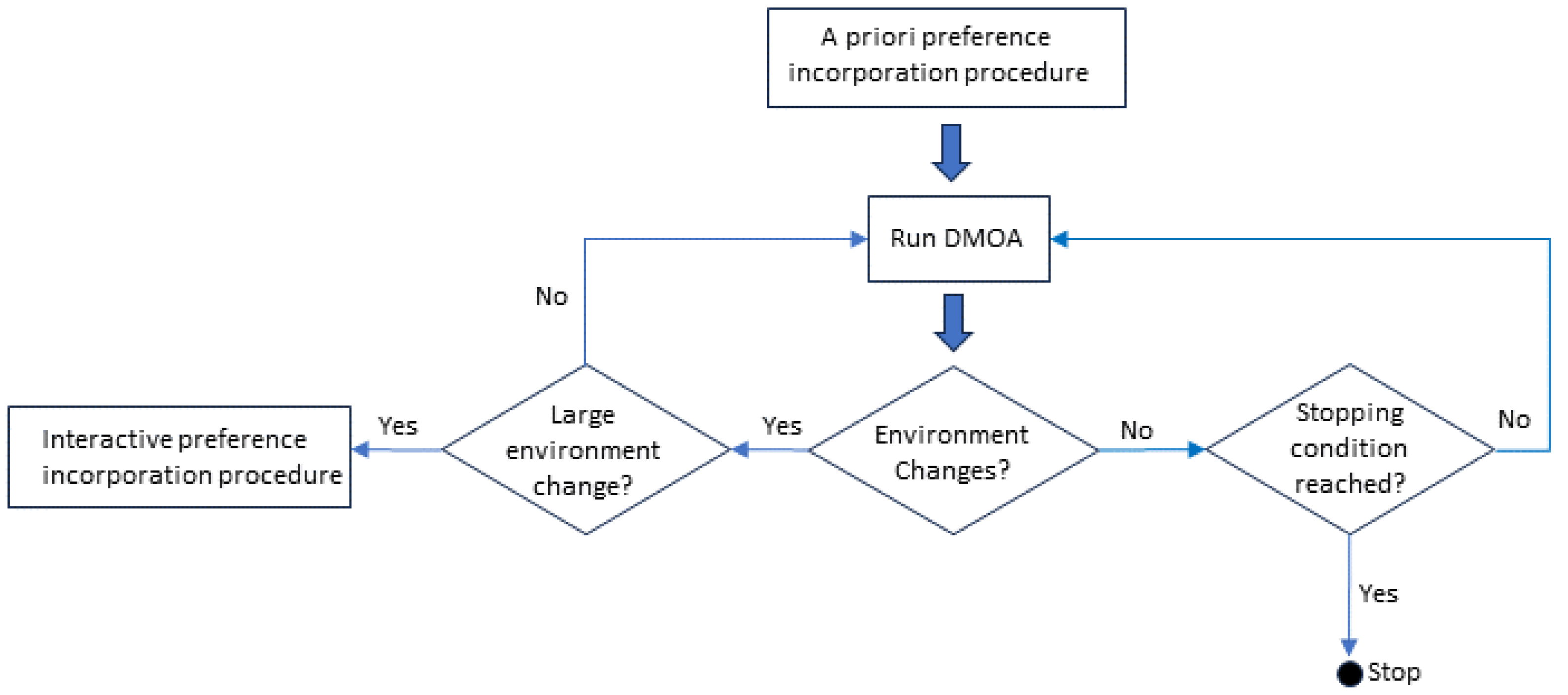
• A preference incorporation method adapted for DMOPs that is partly a priori and partly interactive and enables a DM to specify their preferences. The a priori incorporation of DM preferences occurs through a procedure, named bootstrap. The interactive incorporation of preferences is employed whenever a change occurs in the dynamic environment such that the DM preference set may be significantly affected.
• A bounding box approach (refer to Equation (2) in Section 2) to specify a DM’s preferences in the dynamic multi-objective optimization (DMOO) search process. The proposed bounding box, unlike the proposal in [33], is employed in the context of DMOPs, thus making it the first of its kind.
• New approaches that can drive a DMOA’s search constrained by the DM’s preferences, as well as a comparative analysis of the constraint managing approaches incorporated into a DMOA. The proposed constraint managing approaches are fundamentally different from one another in terms of how they penalize solutions that violate a DM’s preferences.
• New performance measures that measure how well a found solution adheres to the preferences of a DM. In this article, a solution will henceforth be referred to as a decision.

The base DMOA used in this study is a hybrid form of differential evolution (DE) [34], combining non-dominated sorting [35] with vector-evaluation schemes for selecting target vectors and the vectors that survive to the next generation during the optimization process, since it has been shown to perform well in solving DMOPs [36]. The proposed constraint managing approaches are incorporated in the same DMOA (the hybrid DE) to ensure a fair comparison of their performance. Their performance is measured using current (traditional) DMOO measures [1,37,38] and the new measures proposed in this article. It should be noted, however, that the constraint managing approaches and the preferences incorporation approaches can be incorporated into any DMOA.

The rest of the article is organized as follows: Section 2 presents background concepts and theories required to understand the rest of the article. The experimental setup, including the algorithmic setup, benchmark functions, performance measures, and statistical analysis employed in the study are discussed in Section 3. Section 4 presents and discusses the results of the experiments. Finally, conclusions are presented in Section 5 based on the results obtained from the experiments.

2. Background

This section discusses the key concepts which underlie the proposals in this study. Section 2.1 discusses the mathematical formulation of DMOPs that are addressed in this study. It also discusses the mathematics of the proposed bounding box approach and the limiting behaviors of the penalty function employed in this study. Section 2.2 discusses the mathematics required for new performance measures proposed in this article. Lastly, Section 2.3 discusses the core DMOA on which the based DMOA used in this study is based.

2.1. Bounding Box Mathematics

Let a composite function F be defined as follows:

$$F:{\mathsf{\Omega }}_x\times {\mathsf{\Omega }}_t⟶O$$

(1)

where ${\mathsf{\Omega }}_x={\Re }^n$, with $n\ge 2$, refers to the decision space, ${\mathsf{\Omega }}_t\subseteq R$ refers to the time space, $t\in {\mathsf{\Omega }}_t$ is a real-valued time instance and $t={\displaystyle \frac{1}{n_t}}⌊{\displaystyle \frac{\tau }{{\tau }_t}}⌋$, with $n_t$ referring to the severity of change, $\tau$ referring to the iteration counter, and ${\tau }_t$ referring to the frequency of change.

Let the objective space, O, be defined as [39]

$$O=\left\{\begin{array}{cc}{\Re }^2\hfill & (\mathrm{e}.\mathrm{g}.,\mathrm{FDA}1\left[10\right],\mathrm{dMOP}2\left[39\right])\hfill \\ {\Re }^3\hfill & (\mathrm{e}.\mathrm{g}.,\mathrm{FDA}5\left[10\right])\hfill \end{array}\right.$$

Then, a decomposition of F follows:

$$F(\mathbf{x},t)=\left\{\begin{array}{cc}(f1,f2)\hfill & (\mathrm{e}.\mathrm{g}.,\mathrm{FDA}1\left[10\right],\mathrm{dMOP}2\left[39\right])\hfill \\ (f1,f2,f3)\hfill & (\mathrm{e}.\mathrm{g}.,\mathrm{FDA}5\left[10\right])\hfill \end{array}\right.$$

Each objective function $f_i$ is defined as

$$f_i:\left\{\begin{array}{cc}{\mathsf{\Omega }}_x\times {\mathsf{\Omega }}_t⟶R\},\hfill & i=1,2,3\hfill \end{array}\right.$$

Let a DM’s preference set be defined as

$$\mathtt{Box}(\mathbf{z},\mathbf{p})=\{\mathbf{z}\in O|d(\mathbf{z},\mathbf{p})\le r,\mathbf{p}\in O,r\in \Re \}$$

(2)

where d is the Euclidean distance measure, $\mathbf{p}$ is the center of the box formed by the points in this set, $\mathrm{Box}(\mathbf{z},\mathbf{p})$, r is the radius of the box, O is the objective space as defined in Equation (1), and the values of $\mathbf{p}$ and r are interactively selected by the DM.

Let a penalty function and its limiting behaviours be defined as

$$\begin{array}{c}\hfill \mathrm{penalty}({\mathbf{z}}_k\in O,\lambda )=\left\{\begin{array}{cc}0,\hfill & ifd({\mathbf{z}}_k,\mathbf{p})\le r\hfill \\ \lambda (d({\mathbf{z}}_k,\mathbf{p})-r),\hfill & ifd({\mathbf{z}}_k,\mathbf{p})>r\hfill \end{array}\right.\end{array}$$

(3)

$$\begin{array}{c}\hfill \underset{\lambda \to c}{\lim }\mathrm{penalty}({\mathbf{z}}_k\in O,\lambda )=\left\{\begin{array}{cc}0,\hfill & ifd({\mathbf{z}}_k,\mathbf{p})\le r\hfill \\ c(d({\mathbf{z}}_k,\mathbf{p})-r),\hfill & ifd({\mathbf{z}}_k,\mathbf{p})>r\hfill \end{array}\right.\end{array}$$

(4)

$$\begin{array}{c}\hfill \underset{\lambda \to \mathrm{realmax}}{\lim }\mathrm{penalty}({\mathbf{z}}_k\in O,\lambda )=\left\{\begin{array}{cc}0,\hfill & ifd({\mathbf{z}}_k,\mathbf{p})\le r\hfill \\ \mathrm{realmax},\hfill & ifd({\mathbf{z}}_k,\mathbf{p})>r\hfill \end{array}\right.\end{array}$$

(5)

$$\begin{array}{c}\hfill \underset{\lambda \to \mathrm{realmax}}{\lim }{\mathbf{z}}_k+\mathrm{penalty}({\mathbf{z}}_k\in O,\lambda )=\left\{\begin{array}{cc}{\mathbf{z}}_k,\hfill & ifd({\mathbf{z}}_k,\mathbf{p})\le r\hfill \\ I_1·\mathrm{realmax},\hfill & ifd({\mathbf{z}}_k,\mathbf{p})>r\hfill \end{array}\right.\end{array}$$

(6)

$$\begin{array}{c}\hfill \underset{\lambda \to c}{\lim }{\mathbf{z}}_k+\mathrm{penalty}({\mathbf{z}}_k\in O,\lambda )=\left\{\begin{array}{cc}{\mathbf{z}}_k,\hfill & ifd({\mathbf{z}}_k,\mathbf{p})\le r\hfill \\ {\mathbf{z}}_k+I_1·c(d({\mathbf{z}}_k,\mathbf{p})-r),\hfill & ifd({\mathbf{z}}_k,\mathbf{p})>r\hfill \end{array}\right.\end{array}$$

(7)

where $\lambda$ (≥0) is a penalty control parameter whose value is determined by each algorithm, and $\mathbf{p}$, r, and d are defined as in Equation (2).

Then, a penalized outcome, ${\mathbf{z}}_k^{*}\in O$, is defined as ${\mathbf{z}}_k^{*}={\mathbf{z}}_k+I_1·\mathrm{penalty}({\mathbf{z}}_k,\lambda )$ where ${\mathbf{z}}_k$ is a non-penalized outcome in the objective space, ${\mathbf{z}}_k=F({\mathbf{x}}_k,t),{\mathbf{x}}_k\in {\mathsf{\Omega }}_x$, F is as defined in Equation (1), and $I_1$ is an all-ones vector in the objective space (e.g., (1, 1) $\in {\Re }^2$).

2.2. Mathematics for Newly Proposed Performance Measures

This section discusses the mathematics required for two newly proposed performance measures. Section 2.2.1 discusses a measure that calculates the deviation of the violating decisions. The calculation of the spread of non-violating decisions that are found in the bounding box is discussed in Section 2.2.2.

2.2.1. Deviation of Violating Decisions

Solution space vectors whose objective values are outside the preference set are referred to as violating decisions, since they violate DM preferences. Depending on the control parameters used in the implementation of the penalty function of the proposed algorithms, the violating decisions may occasionally find their way into the archive, especially in situations where all the non-dominated solutions violate DM preferences and non-violating decisions are not found. However, it is a rare scenario: the non-violating decisions, if they are found in the archive, are very likely to dominate the violating and penalized decisions in the Pareto-dominance sense. However, when violating decisions find their way into the archive, a measure of the proximity of these violating decisions to the preferred bounding box is required. The smaller the total proximity, the better the violating decisions are. This section presents the mathematics underlying the calculation of the total proximity/deviation of the violating decisions.

Let $\mathbf{p}$, r, and the distance measure $d(\mathbf{z},\mathbf{p})$ be as defined in Section 2.1, and let a set of violating decisions, Z, be defined as follows:

$$Z=\{{\mathbf{z}}_k\in O|d(\mathbf{z},\mathbf{p})>r\},k=1,\dots ,\left|Z\right|$$

(8)

Let the cardinality, N, of Z be defined as

$$N=\left|Z\right|$$

(9)

Let the deviation of ${\mathbf{z}}_k\in Z$ be defined as

$$d_k=d({\mathbf{z}}_k,\mathbf{p})-r(d_k>0)$$

(10)

Then the total deviation of all elements in Z is

$$\mathrm{dVD}=\sqrt{\frac{\sum {(1+d_k)}^2}{N}}$$

(11)

2.2.2. Spread of Non-Violating Decisions

The spread of non-violating decisions is one of the four measures proposed in this article. This measure estimates how well spread out the preferred decisions are within the bounding box located in the objective space. The greater the value of this measure, the better the performance of an algorithm. The calculation of this measure is presented in Algorithm 1.

Algorithm 1 Spread of Non-violating decisions
1: procedure SpreadEstimator(outcomes)     ▹ outcomes: objective vectors preferred by DM
2:     Get count of outcomes, N $\leftarrow \mathrm{count}\left(\mathrm{outcomes}\right)$
3:     if $\mathrm{N}\le 1$ then
4:         return 0	▹ 1 or zero outcomes, spread is zero
5:     if $\mathrm{N}==2$ then	▹ 2 outcomes
6:         return norm${}_2(\mathrm{outcomes}\left(2\right)-\mathrm{outcomes}\left(1\right))$	▹ return spread between 2 values
7:     dtot $\leftarrow 0$	▹ more than 2 outcomes, calculation required - initialize total spread, $dtot$
8:      firstNode ← outcomes(1)	▹ get a node
9:      currentNode ← firstNode	▹ set current node
10:     while $\mathrm{unProcessedNodes}\left(\mathrm{outcomes}\right)>1$ do	▹ process each outcome
11:         MarkNodeAsProcessed(currentNode)	▹ mark outcome as processed
12:         nearestNode=getNearestNode(currentNode,outcomes)	▹ find nearest node to outcome being processed
13:         dist = $nor{m}_2(\mathrm{currentNode}-\mathrm{nearestNode})$	▹ calcuated distance between these two solutions
14:          dtot ← dtot + dist	▹ add their distance to total distance
15:          currentNode ← nearestNode
16:     dist = $nor{m}_2(\mathrm{currentNode}-\mathrm{firstNode})$	▹ finally calculate distance to first solution
17:      dtot ← dtot + dist	▹ add last distance to total distance
18:     return dtot	▹ return total distance

2.3. Core Dynamic Multi-Objective Optimization Algorithm

The core DMOA used in this study is presented in Algorithm 2. The algorithm starts with a set of randomly generated solutions, after initializing its run-time parameters, such as the population size, maximum archive size, maximum number of iterations, etc. The non-dominated solutions are added to the archive. A loop is performed until the number of iterations exceeds the maximum number of iterations. The non-dominated solutions, which are found at the end of the loop’s execution, constitute the final solutions to the associated optimization problem. The algorithm uses sentry solutions to check whether a change in the environment has occurred.

Algorithm 2 Dynamic Multi-objective Optimization Algorithm
1: procedure DMOA(freq, severity, maxiteration, dMOP)
2:     Set population size, N
3:     Set archive max size, SizeArchive
4:     Initialize the iteration counter, $\mathrm{iteration}\leftarrow 0$
5:     Initialize time, $\mathrm{t}\leftarrow 0$
6:     Initialize(${\mathrm{P}}_t,\mathrm{freq},\mathrm{severity},\mathrm{dMOP},\mathrm{t}$)	▹ initialize population of solutions, $P_t$
7:     AssignNonDominatedToArchive(P${}_t$, dMOP, t)	▹ initialize archive
8:     while iteration ≤ maxiteration do	▹ check if stopping condition has been reached
9:         t $\leftarrow 1/\mathrm{severity}·\lfloor \mathrm{iteration}/\mathrm{freq}\rfloor$	▹ calculate the current time
10:         Optimizer(P${}_t$, dMOP, t)	▹ perform the search optimization
11:         Pick sentry solutions	▹ select sentry solutions to check for change
12:         if ENV changes(P${}_t$, dMOP, t) then	▹ check for change in environment
13:            ProcessChange(P${}_t$, freq, severity, dMOP, t)	▹ respond to change
14:         iteration ← iteration$+1$	▹ increase iteration count

3. Experimental Setup

This section discusses the experimental setup used for this study. Section 3.1 discusses the algorithm setup. The DM preferences are discussed in Section 3.2. Section 3.3 discusses the benchmark functions, and the performance measures are highlighted in Section 3.4. The statistical analysis approach is discussed in Section 3.5.

3.1. Algorithm Setup

The approach that was followed to incorporate the DM’s preference into the search process of the DMOA is discussed in Section 3.1.1.

3.1.1. Decision-Maker’s Preference Incorporation

The different procedures and how they are used with a DMOA for the preference-driven search process are presented in Figure 1. Before the normal run of the DMOA starts, the a priori preference incorporation procedure is used to define the DM’s preference. During the run of the DMOA, any of the constraint managing approaches can be used. If a small environment change occurs, the DMOA’s change response approach is executed during the normal DMOA run. However, if the change is large, requiring a change in the boundary box placement, the interactive preference incorporation procedure is first completed before the DMOA’s change response approach is executed during the normal DMOA run.

Figure 1. Preference-driven search process of a DMOA.

A Priori Preference Incorporation: A single run of the algorithm is executed. A series of POFs is presented to the DM. The DM selects one of these POFs, and then selects one of the points on the POF, which will become his ${\mathbf{x}}_p$ and $\mathbf{p}$, i.e., the preferred decision/solution vector and the preferred outcome, respectively. This preference, together with the radius of the bounding box specified by the DM during the bootstrap procedure (refer to Algorithm 3), is used to drive the DMOA’s search to optimize the DMOPs under the constraints of the DM’s preferences. The time complexity of the bootstrap procedure is similar to the time complexity of the DMOA that is used to produce the POSs.

Algorithm 3 Bootstrap Procedure
1: procedure BootStrap(freq, severity, iteration, F)
2:     Call DMOA(freq, severity, iteration, F)    ▹ DMOA returns $\left\{{\mathrm{POS}}_t^k\right\},\forall k=1,\dots ,n$    ▹ where k is the kth environment change
3:     $\mathrm{i}\leftarrow \mathrm{DMChooseIn}(1,\dots ,n)$	▹ DM indicates their preferred POS
4:     ${\mathrm{x}}_p\leftarrow \mathrm{DMChooseIn}\left(PO{S}_t^i\right)$	▹ DM indicates their preferred solution
5:     $\mathrm{p}\leftarrow \mathrm{F}({\mathrm{x}}_p,\mathrm{t})$	▹ DM’s preference is formulated
6:     DM Choose box radius, r ← random()	▹ DM indicates their preferred boundary box size
7:     return (x${}_p$ : p : r)

Interactive Preference Incorporation: A significant change in the environment may occur where the resulting POF may shift in such a way that the DM preference, $\mathbf{p}$, is no longer part of the new POF. In this scenario, the DM interactively redefines the position of the bounding box ensuring that its preference lies on the new POF. A few scenarios may emerge when this shift of the POF occurs. The initial preferred outcome, p, may no longer lie on the new POF, but the functional value of the corresponding decision variable, $x_p$, may still lie on the new POF. The second possibility is that both p and the functional value of $x_p$ do not lie on the new POF. In both cases, a new bounding box position needs to be defined. The interactive redefinition of the bounding box position is presented in Algorithm 4. The time complexity of the interactive preference incorporation procedure is a constant value, i.e., low time complexity.

Algorithm 4 Interactive Incorporation of Preferences
1: procedure RepositionBoundingBox(F, x${}_p$, p, r, t)     ▹ F: multi-objective function to be evaluated     ▹ x${}_p$: DM preferred decision vector     ▹ p: DM preferred outcome as defined in Equation (2), page 3     ▹ r: DM preferred box radius     ▹ Archive: ${\mathrm{POS}}_t$
2:     ${\mathrm{POF}}_t\leftarrow \mathrm{F}({\mathrm{POS}}_t,\mathrm{t})$	▹ POF is corresponding objective values of POS
3:     if p $\in {\mathrm{POF}}_t$ then	▹ DM preferred outcome still lies on POF
4:          return (x${}_p$:p:r)
5:     if F(x${}_p$,t) ∈ POF${}_t$ then	▹ DM’s preferred decision lies on POF, preferred outcome does not
6:         Reposition center of box, p ← F(x${}_p$, t)	▹ Automatically reposition center of box
7:          return (x${}_p$:p:r)
8:     $x_p\leftarrow \mathrm{DMChooseIn}\left(PO{S}_t\right)$	▹ DM selects a new position for $x_p$ and p
9:     Reposition center of box, $\mathrm{p}\leftarrow F(x_p,\mathrm{t})$	▹ Reposition center of box based on DM’s input
10:      return ($x_p:\mathrm{p}:\mathrm{r}$)

3.1.2. Algorithms

The following three approaches employ a penalty function (refer to Equation (3), Section 2) to penalize violating decisions which do not satisfy the DM’s preferences. Each of these approaches were incorporated into the hybrid DE and are the three constraint managing approaches evaluated in this study:

• Proportionate Penalty: With this approach, the penalty is proportional to the violation, and violating decisions are penalized during function evaluation. Algorithm 5 presents this approach, referred to as PPA for the rest of the article.

  Algorithm 5 Proportionate Penalty Algorithm
  1: procedure FuncEvaluate(F, x, t)     ▹ F: multi-objective function to be evaluated     ▹ x: decision vector     ▹ p: as defined in Equation (2), page 3     ▹ r: as defined in Equation (2), page 3     ▹$\lambda$: as defined in Equation (2), page 3     ▹$\lambda$: a random number between 100 and 1000     ▹$I_1$: as defined in Equation (2), page 3
  2:     z ← F(x,t)	▹ calculate objective value of x
  3:     d $\leftarrow nor{m}_2$(z-p) − r	▹ calculate violation of z
  4:     if d ≤ 0 then
  5:         return z	▹ x is a non-violating decision, no penalty applied
  ▹ x is a preference violating decision, proceed to penalize it for violation
  6:     penalty $\leftarrow \lambda ·$ d	▹ calculate penalty
  7:     penalty ← I${}_1·$ penalty	▹ vectorize penalty
  8:     z ← z + penalty	▹ impose proportionate penalty to objective value of x
  9:     return z	▹ return new penalized objective value of x

• Death Penalty: Maximum/death penalty is imposed on violating decisions during function evaluation. Some penalty, which is death, is administered on a decision irrespective of the magnitude of the violation of that decision. With maximum penalty, it becomes very unlikely that violating decisions will find their way into the archive, because they will be dominated by non-violating decisions. Violating decisions are computationally eliminated during the search process, and the optimization process is driven towards a region of the search space dominated by non-violating decisions. The Death Penalty Algorithm, referred to as DPA in the rest of the article, is presented in Algorithm 6.

  Algorithm 6 Death Penalty
  1: procedure FuncEvaluate(F, x, t)     ▹ F: multi-objective function to be evaluated     ▹ x: decision vector     ▹ p: as defined in Equation (2), page 3     ▹ r: as defined in Equation (2), page 3     ▹$I_1$: as defined in Equation (2), page 3     ▹ realmax: maximum real value on a machine
  2:     z ← F(x,t)	▹ calculate objective value of x
  3:     d $\leftarrow nor{m}_2$(z-p) − r	▹ calculate violation of z
  4:     if d ≤ 0 then
  5:         return z	▹ x is a non-violating decision, no penalty applied
  ▹ x is a preference violating decision, proceed to penalize it for violation
  6:     penalty ← realmax	▹ calculate penalty
  7:     penalty ← I${}_1·$ penalty	▹ vectorize penalty
  8:     z ← penalty	▹ impose death/max penalty
  9:     return z	▹ return new penalized objective value of x

• Restrict Search To Feasible Region: Feasibility is preserved by starting the search within the preferred bounding box and employing the death penalty to prevent preference violating decisions from entering the archive. This approach restricts the search to the feasible region, unlike [40], and it improves the exploring capability of this algorithm. Preferred decisions start the search during initialization of the population of decisions. A pool of preferred decisions is aggregated with the DM preference and the current decisions in the archive. Then, a loop is performed where nearly identical clones of the pool of preferred decisions are created using polynomial mutation [41]. These new clones constitute a new population from where the search will start. Some of the non-dominated decisions in the new population are added to the archive. Algorithm 7 presents the Restrict Search To Feasible Region Algorithm, referred to as RSTFRA in the rest of the article.

  Algorithm 7 Restrict Search to Feasible Region
  1: procedure Initialize($P_t,freq,severity,F,t$)     ▹ x${}_p$: DM preferred decision vector)     ▹ archive: POS     ▹ F: multi-objective function to be evaluated     ▹ N: population size, fixed for this study
  2:     pool ← [x${}_p$ ; archive]	▹ pooled preferences
  3:     i ← 1	▹ initialize counter
  4:     while i ≤ N do
  5:         iNumberAttempts ← 1
  6:         while (iNumberAttempts ≤ 100) && (!isPreferredDecision(solution, F, t) ) do	▹ searching for prefered decision
  7:            solution ← randomlyChooseIn(pool)	▹ randomly select solution from pool
  8:            solution ← polynomial_mutate(solution)	▹ apply mutation to solution
  9:            iNumberAttempts ← iNumberAttempts + 1	▹ increment number of attempts
  10:         addSolutionToPopulation(P${}_t$, solution)	▹ add mutated solution to the population
  11:         i ← i + 1
  12:     AssignNonDominatedToArchive(P${}_t$, F, t )	▹ add non-dominated decisions to archive

The time complexity of the constraint managing approaches PPA and DP is a constant value. The time complexity of RSTFRA is $O\left(m\right)$ due to adding the non-dominated solution to the archive with size m.

3.1.3. Differential Evolution Algorithm Control Parameters

The following settings were used for the DE algorithm in this study:

• The base algorithm (refer to Algorithm 8) is characterized as DE/best/1/bin.
• To generate a trial vector from a parent vector during the mutation phase of the algorithm, the best vector in the adjacent hypercube or sub-population of the parent vector is selected as the target vector. The number of hypercubes employed by the algorithm is the same as the number of objective functions in the underlying DMOP.
• Two randomly selected vectors from the parent vector’s hypercube are used to form a difference vector.
• Binary crossover [42] is used due to its viability as a crossover method in DE algorithms.
• The scaling factor, $\beta$, amplifies the effects of the difference vector. It has been shown that a larger $\beta$ increases the probably of escaping local minima, but can lead to premature convergence. On the other hand, a smaller value results in smaller mutation step sizes slowing down convergence, but facilitating better exploitation of the search space [43,44]. This leads to a typical choice for $\beta$ in the range $(0.4,0.95)$ [43,44]. Therefore, in this study, the algorithm randomly chooses $\beta \in (0.4,1)$. The recombination probability is $p_r=0.8$, since DE convergence is insensitive to the control parameters [42,45] and a large value of $p_r$ speeds up convergence [43,45,46].

Algorithm 8 Differential Evolution Algorithm
1: procedure Optimizer(P, F, t)     ▹$\beta$: scaling factor set per algorithm     ▹ p${}_r$: recombination prob set per algorithm     ▹ maxgen($\ge 1)$: number of function evaluations set per algorithm     ▹ P: current population of vectors     ▹ F: multi-objective function to be optimized     ▹ t: current time
2:     gen = 1	▹ set the generation counter
3:     P${}_{gen}\leftarrow$ P	▹ initialize current population
4:     V ←Ø	▹ initialize set of vectors
5:     while gen ≤ maxgen do	▹ check if stopping condition has been reached
6:         while moreUnprocessed(v ∈ P${}_{gen}$) do	▹ process all individuals of population
7:              v${}^{{}^{\prime }}\leftarrow$ getTrialVector($\beta$, v, P${}_{gen}$, F, t)	▹ calculate trial vector
8:              v${}^{{}^{″}}\leftarrow$ getChildVector(p${}_r$, v${}^{{}^{\prime }}$, v, F, t)	▹ produce child vector
9:              V ← V ∪ {v, v${}^{{}^{″}}$}	▹ add trial and child vectors to set of vectors
10:             markAsProcessed(v ∈ P${}_{gen}$)
11:         P${}_{gen}\leftarrow$ getNextGenerationVectors(V)	▹ produce next generation
12:         gen ← gen+1	▹ increment counter
13:         V ←Ø	▹ reset set of vectors
14:     AssignNonDominatedToArchive(P${}_{maxgen}$, F, t )	▹ add non-dominated solutions to archive

The time complexity of the static non-dominated sorting genetic algorithm II (NSGA-II) is $O\left(i{N}^2\right)$, where i is the number of objective functions and N is the population size [35]. The non-dominated sorting has a time complexity of $O\left(i{N}^2\right)$, the crowding distance calculation has a time complexity of $O(iNlogN$), and elitist sorting has a time complexity of $O\left(i{N}^2\right)$ [35].

The DE algorithm used in this study uses the same non-dominated sorting and elitist sorting as NSGA-II. In addition, the time complexity of adding a solution to the archive is $O\left(im\right)$, where m is the size of the archive. When a change in the environment occurs, the re-evaluation of the archive has a time complexity of $O\left(i{m}^2\right)$. However, it should be noted that all DMOAs that incorporate a change response would typically re-evaluate the solutions. Therefore, the time complexity of the DE is $O\left(i{m}^2\right)$. Furthermore, since the base algorithm used in this study is only for demonstration purposes, if these approaches are incorporated into another DMOA, the time complexity will depend on that of the chosen DMOA.

3.2. Decision-Maker’s Preferences

The DM preferences are correspondingly associated, serially, with each of the eighteen experimental configurations in Section 3.3. For instance, the first experimental preference in Table 1 is associated with the first experimental preference in Table 2, while both are associated with the first experimental configuration in Table 3.

Table 1. Experimental preferences for decision variables.

S/N	${\mathit{x}}_1$	${\mathit{x}}_2$	${\mathit{x}}_3$	${\mathit{x}}_4$	${\mathit{x}}_5$	${\mathit{x}}_6$
1	0.47600	0.53000	0.5877	0.59104	0.5324	0.4989
2	0.47700	0.33000	0.1630	0.42817	0.3250	0.2654
3	0.47600	0.19000	0.0912	0.17928	0.1616	0.2331
4	0.81600	0.95000	0.8768	0.86623	0.4892	0.7924
5	0.76100	−0.10000	0.1513	−0.17267	0.0387	0.1229
6	0.16700	0.18000	0.0032	−0.00311	0.1462	−0.0284
7	0.96400	3.5 × 10${}^{-6}$	0.5378	0.51880	0.3188	0.5433
8	0.00000	2.8 × 10${}^{-5}$	0.3660	0.28965	0.4592	0.3918
9	1.00000	0.00030	0.3992	0.39925	0.5292	0.4621
10	0.35700	1.00000	0.5083	0.74667	0.8383	0.7472
11	0.00000	0.00091	0.7330	0.49810	0.8207	0.6616
12	0.00000	0.08000	0.6419	0.87802	0.8485	0.8020
13	0.14600	0.31000	0.2970	0.30878	0.3052	0.3065
14	0.73400	0.16000	0.1657	0.13508	0.1101	0.1729
15	0.31700	0.31000	0.3230	0.32197	0.3290	0.2881
16	0.06100	0.00460	0.0027	0.00225	0.0032	0.0079
17	1.00000	0.04400	0.0391	0.10593	0.0204	0.0658
18	0.00000	0.00280	0.0015	0.00042	0.0016	0.0045

Table 2. Experimental preferences for objective values.

S/N	${\mathit{f}}_1$	${\mathit{f}}_2$	${\mathit{f}}_3$
1	0.4800	0.3200	N/A
2	0.4800	0.6200	N/A
3	0.4800	0.9300	N/A
4	0.8200	2.4000	N/A
5	0.7600	0.1700	N/A
6	0.1700	0.6300	N/A
7	0.9300	4.5 × 10${}^{-71}$	1.3843
8	1.8000	2.9 × 10${}^{-59}$	0
9	1.0 × 10${}^{-16}$	4.5 × 10${}^{-62}$	1.6781
10	2.8 × 10${}^{-8}$	2.8 × 10${}^{-8}$	1.6354
11	2.9000	0.0041	0
12	3.5000	0.4400	0
13	0.1500	4.6000	N/A
14	0.7300	9.5000	N/A
15	0.3200	4.3000	N/A
16	0.0610	0.9700	N/A
17	1.0000	0.2100	N/A
18	0.0000	1.0000	N/A

Table 3. Benchmark function configurations.

S/N	DMOP	${\mathit{\tau }}_{\mathit{t}}$	${\mathit{n}}_{\mathit{t}}$	Iterations	c(f(x))	$\mathit{\sigma }\left(\mathbf{runs}\right)$
1	FDA1	4	10	16	20	30
2	FDA1	5	10	20	20	30
3	FDA1	2	10	8	20	30
4	FDA1	4	1	16	20	30
5	FDA1	5	1	20	20	30
6	FDA1	2	1	8	20	30
7	FDA5	4	10	16	20	30
8	FDA5	5	10	20	20	30
9	FDA5	2	10	8	20	30
10	FDA5	4	1	16	20	30
11	FDA5	5	1	20	20	30
12	FDA5	2	1	8	20	30
13	dMOP2	4	10	16	20	30
14	dMOP2	5	10	20	20	30
15	dMOP2	2	10	8	20	30
16	dMOP2	4	1	16	20	30
17	dMOP2	5	1	20	20	30
18	dMOP2	2	1	8	20	30

3.3. Benchmark Functions

Three DMOPs with various ${\tau }_t$-$n_t$ combinations were used in this study. The experimental configurations used for these benchmarks are presented in Table 3.

The following symbols were used in Table 3: ${\tau }_t$: frequency of change; $n_t$: severity of change; $c\left(f\right(x\left)\right)$: count of function evaluations per iteration; $\sigma \left(runs\right)$: number of runs per configuration; $FDA1$: type I DMOP (POS is dynamic, POF is static), POF = $1-\sqrt{f_1}$ and is convex, POS is $x_i=G\left(t\right)$ [10,38]; $FDA5$: type II DMOP (POS and POF are dynamic), for 3 objectives, POF = $f_1^2+f_2^2+f_3^2={(1+G\left(t\right))}^2$ and is non-convex, POS is $x_i=G\left(t\right)$ [10,38]; $dMOP2$: POF changes from convex to concave, type II DMOPs, POF = $1-f_1^{H\left(t\right)}$, POS is $x_i=G\left(t\right)$ [38,39].

3.4. Performance Measures

Each of the performance measures were calculated immediately before a change in the environment occurred. This was performed for thirty runs. An average of the values of the thirty runs was then calculated for each measure in each environment.

The following traditional DMOO performance measures were used in this study:

• Accuracy (acc) measures how accurately a DMOA is able to approximate the true POF of a DMOP [1,37,38]. The lower the value of acc, the better the performance of the DMOA.
• Stability (stab) quantifies the effect of environment changes on the accuracy measure value [1,37,38,47]. The lower the value of this measure, the better the DMOA’s performance.
• Hypervolume Ratio (hvr) [48] measures the proportion of the objective space that is covered by a non-dominated set without suffering from the bias of a convex region as seen with the hypervolume measure [49]. The higher the value of this measure, the better the DMOA’s performance.
• Reactivity (react) [50] measures how long it takes a DMOA to recover after a change in environment occurred, i.e., the length of time it takes to reach a specified accuracy threshold after the change occurred [38]. The lower the value of this measure, the better the DMOA’s performance.

The following newly proposed measures were used in this study:

• Number of Non-Violating Decisions (nNVD) measures the number of decisions that fall within the DM’s preference set. The higher the value of this measure, the better a DMOA’s performance.
• Spread of Non-Violating Decisions (sNVD) measures the spread of decisions within the preference set. A high value indicates a good DMOA performance.
• Number of Violating Decisions (nVD) measures the number of violating decisions in the archive. These are decisions that do not lie within the preference set. The lower the value of this measure, the better the performance of the DMOA.
• Total Deviation of Violating Decisions (dVD) measures the total deviation from the preference set for all violating decisions in the archive. It is calculated based on the steps that are highlighted in Section 2.2.1. The lower the value of this measure, the better the DMOA’s performance.

The four new performance measures proposed in this article specifically measure the performance of a DMOA with regards to DM preference constraints, and thus facilitate the comparative analysis of DMOAs in the context of a DM’s preferences.

3.5. Statistical Analysis

A statistical analysis of the performance measure values was conducted in accordance with the wins-losses${}_B$ algorithm proposed in [1]. The wins-losses${}_B$ algorithm was implemented in R [51], and the Kruskal–Wallis and Mann–Whitney U statistical functions in R were used as stipulated in [1]. The calculation of wins and losses by the wins-losses${}_B$ algorithm is presented in Algorithm 9 [52].

A win or loss is only recorded if there was a statistical significant difference in performance of the two algorithms that are being compared with the pair-wise Mann–Whitney U test. Therefore, $Diff>0$ indicates a good performance, since the DMOA obtained more wins than losses. On the other hand, $Diff<0$ indicates a poor performance, since the DMOA was awarded more losses than wins.

Algorithm 9 wins-losses${}_B$ algorithm for wins and losses calculation [52]

1: for each benchmark do 2:     for each $n_t$-${\tau }_t$ combination do 3:         for each performance measure, $p_m$ do 4:            for each algorithm $alg$ do 5:                Calculate the average value $p{m}_{avg}$ for each of the 30 runs 6:                Perform Kruskal–Wallis test on the average values, $p{m}_{avg}$ 7:                if statistically significant difference then 8:                    for each pair of algorithms do 9:                        Perform Mann–Whitney U test 10:                        if statistically significant difference then 11:                           for each environment $env$ do 12:                               Assign a win to algorithm with best average over all 13:                                  $p{m}_{avg}$ for $env$ 14:                               Assign a loss to algorithm with worst average over all 15:                                  $p{m}_{avg}$ for $env$ 16: Calculate $Diff=\#wins-\#losses$ ▹ calculate $Diff$ for each parameter (benchmark, $n_t$-${\tau }_t$ combination, performance measure, algorithm) as required for analysis

4. Results

This section presents a summary of the results obtained from this study. Detailed results are, however, presented in Appendix A.

The summarized results are presented in Table 4, Table 5 and Table 6. For all of these tables, any column with a bold entry signifies the winning algorithm for the particular measure of performance, or for the experimental configuration, in the corresponding row.

Table 4. Overall wins and losses for various frequency and severity of change combinations using wins-losses${}_B$ [1].

${\mathit{n}}_{\mathit{t}}$	${\mathit{\tau }}_{\mathit{t}}$	RESULTS	PPA	DPA	RSTFRA
10	4	Wins	64	59	53
10	4	Losses	54	58	64
10	4	Diff	10	1	−11
10	4	Rank	1	2	3
10	5	Wins	61	67	32
10	5	Losses	45	40	75
10	5	Diff	16	27	−43
10	5	Rank	2	1	3
10	2	Wins	73	60	35
10	2	Losses	40	54	74
10	2	Diff	33	6	−39
10	2	Rank	1	2	3
1	4	Wins	41	67	56
1	4	Losses	66	44	54
1	4	Diff	−25	23	2
1	4	Rank	3	1	2
1	5	Wins	56	73	43
1	5	Losses	53	47	72
1	5	Diff	3	26	−29
1	5	Rank	2	1	3
1	2	Wins	51	77	55
1	2	Losses	64	49	70
1	2	Diff	−13	28	−15
1	2	Rank	3	1	2

Table 5. Overall Wins and Losses for various performance measures, and frequency and severity of change combinations, using wins-losses${}_B$ [1].

PM	RESULTS	PPA	DPA	RSTFRA
acc	Wins	69	83	63
acc	Losses	75	60	80
acc	Diff	−6	23	−17
acc	Rank	2	1	3
stab	Wins	23	23	32
stab	Losses	22	34	22
stab	Diff	1	−11	10
stab	Rank	2	2	1
hvr	Wins	82	94	40
hvr	Losses	62	50	104
hvr	Diff	20	44	−64
hvr	Rank	2	1	3
react	Wins	14	45	45
react	Losses	57	25	22
react	Diff	−43	20	23
react	Rank	3	1	1
nNVD	Wins	91	65	39
nNVD	Losses	38	67	90
nNVD	Diff	53	−2	−51
nNVD	Rank	1	2	3
sNVD	Wins	67	87	47
sNVD	Losses	68	48	85
sNVD	Diff	−1	39	−38
sNVD	Rank	2	1	3
nVD	Wins	0	2	4
nVD	Losses	0	4	2
nVD	Diff	0	−2	2
nVD	Rank	3	2	1
dVD	Wins	0	4	4
dVD	Losses	0	4	4
dVD	Diff	0	0	0
dVD	Rank	3	1	1

Table 6. Overall wins and losses for various DMOA using wins-losses${}_B$ [1].

RESULTS	PPA	DPA	RSTFRA
Wins	346	403	274
Losses	322	292	409
Diff	24	111	−135
Rank	2	1	3

Figure 2 and Figure 3 present the objective space for a selected DMOP which is constrained by a bounding box representing a DM’s preferences for two selected experimental configurations. The bounding box in these specific instances is a sphere. The two figures present the results for a randomly chosen run and a randomly chosen environment among many environments (changes) that are typical of a single run of a DMOA solving a DMOP.

Figure 2. Decisions found by DPA (above) and RSTFRA (below) for FDA5 with Sphere Spec = $(1.7808,2.9185\times {10}^{-59},0.0,1.5)$, $n_t=10$ and ${\tau }_t=5$.

Figure 3. Decisions found by DPA (above) and PPA (below) for FDA5 with Sphere Spec = $(1.0276\times {10}^{-16},4.4955\times {10}^{-62},1.68781,1.5)$, $n_t=10$ and ${\tau }_t=2$.

Table 4 presents the results for six experimental configurations, for various $n_t$–${\tau }_t$ combinations, i.e., different types of environment changes. It highlights the total number of wins and losses obtained by each constraint managing approach (algorithm) over all benchmarks and measures for each of the environment types. The death-penalty algorithm (DPA) performed the best for four types of environments ($n_t$–${\tau }_t$ combinations), while the proportionate-penalty algorithm (PPA) outperformed the other DMOAs in the other two environment types ($n_t=10,\tau =2$ and $n_t=10,\tau =4$). In those six $n_t-{\tau }_t$ combinations, the RSTFRA never outperformed DPA but it performed better than PPA in two types of environments ($n_t=1,\tau =4$ and $n_t=1,\tau =2$). DPA was the only DMOA that obtained more wins than losses for all environment types. The Restrict-search-to-feasible-region algorithm (RSTFRA) obtained more losses than wins for all environment types, except for $n_t=10,\tau =2$. On the other hand, PPA obtained more wins than losses for all environments, except $n_t=1,\tau =4$ and $n_t=1,\tau =2$.

Table 5 presents the performance of the proposed algorithms with respect to the performance measures discussed in Section 3.4. It highlights the total number of wins and losses obtained by each algorithm for all the benchmarks and environment types for each of the performance measures. DPA performed the best for five of the eight measures and second-best for the rest. Two (react and dVD) of its five wins were ties with RSTFRA. Results for the first four measures in Section 3.4 indicated that DPA performed the best for three (acc, hvr, react) out of the four measures. It won with the least number of losses for the accuracy measure, acc, making it the most accurate of the proposed algorithms. For those four measures, RSTFRA won once (stab), but obtained the same number of losses as PPA for the win. RSTFRA also obtained the highest number of worst rankings. None of the algorithms obtained more wins than losses for all of the measures, with all algorithms obtaining more losses than wins for at least three measures.

DPA had the highest number of wins for the measures proposed in this study, i.e., it performed the best for two out of four measures, making DPA the best performing algorithm for all the performance measures discussed in Section 3.4. PPA recorded the highest number of wins for the nNVD measure, while DPA ranked first for the sNVD measure. Thus, PPA and DPA performed better than RSTFRA in finding non-violating decisions of a DM’s preferences. Although RSTFRA ranked best for nVD and dVD, the magnitude of wins recorded by RSTFRA for those two measures were negligible. Despite RSTFRA ranking first for nVD and dVD, PPA never lost to any of the other algorithms on those measures. DPA tied with RSTFRA on the dVD measure.

Table 6 presents the overall results, presenting the total number of wins and losses obtained by each algorithm over all performance measures and all environment types for all benchmarks. PPA ranked first with 403 wins, DPA recorded 346 wins, while RSTFRA ranked last with 274 wins. In addition, RSTFRA recorded the highest number of overall losses (409), resulting in the most negative $Diff$ value. DPA recorded the least number of overall losses and the most positive $Diff$ value. These overall results are consistent with the earlier results, which indicate that DPA performed the best on most of the performance measures and $n_t-{\tau }_t$ combinations, while RSTFRA consistently lagged behind the other two proposed algorithms.

Figure 2 and Figure 3 present the objective space where the preferred objective vectors, or preferred outcomes, are contained in a DM’s preference set. The preference set, or the bounding box, in these instances is a sphere whose defining properties are specified by a DM in the bootstrap procedure described in Algorithm 3. For the sphere specifications in Figure 2 and Figure 3, the first three numbers represent the location of the center of the sphere, while the last number represents the radius of the sphere.

Figure 2 and Figure 3 are simply snapshots and are thus incapable of showing the dynamics of the preference set. They are, however, presented in this section to provide a one-time view into the state of the objective space during the optimization process.

In all the snapshots presented by Figure 2 and Figure 3, all the decisions in the archive are preferred by the DM, since all the objective vectors lie within the spheres representing the DM’s preferences. This is a testament to the fact that the proposed algorithms are effective in finding optimal trade-off solutions/decisions that reflect a DM’s preferences within the search space.

DPA in Figure 2 had the highest number of preferred vectors/outcomes within its spheres, which is consistent with earlier results in this section, indicating its overall superiority over the other algorithms proposed in this study. As a matter of fact, it is ranked best for the experimental configuration represented by Figure 2, and RSTFRA is ranked the worst performing algorithm.

In the experimental configuration represented by Figure 3, PPA ranked best, though only marginally better than DPA. Both algorithms effectively found the DM’s preferred decisions, as none of the algorithms produced violating decisions.

5. Conclusions

This article investigated the incorporation of a DM’s preferences when solving DMOPs. The following contributions were made: an approach that is partly a priori and partly interactive that enables a decision-maker to indicate its preferences for dynamic problems; a bounding box approach to incorporate the preferences in the DMOA’s search; constraint managing approaches to drive the search of a DMOA constrained by the preferences; and new performance measures measuring how well a DMOA’s found solutions adhere to the preferences of a DM.

The results show that a DM’s preferences can effectively be specified using the proposed approach which is partly a priori and interactive. The results further indicate that the proposed bounding box specification is an effective mathematical abstraction of a DM’s preferences. The three proposed constraint managing approaches showed varying degree of performance. The DPA performed the best, while RSTFRA lagged behind the other proposed approaches. Furthermore, the four new performance measures proposed in this article that specifically evaluate the performances of DMOAs in the context of a DM’s preferences proved to effectively evaluate the performance of the DMOAs.

Future work will include experimenting with some of the geometric properties of the bounding box and the impact that these properties have on being able to specify the preferences of the DM in various ways.

It will not be trivial to compare the performance of different approaches that define a decision-maker’s preferences in the traditional way that DMOAs’ performance is evaluated. The way in which a specific approach defines the decision-maker’s preferences will directly influence the solutions that a DMOA finds. This article took the first step towards this, by proposing new performance measures for measuring the performance of DMOAs based on how well their found solutions adhere to the DM’s preferences. However, the question remains: if you compare two approaches that incorporate decision-maker preferences, how will you be able to determine whether one will be better than the other? As long as both approaches find solutions that do adhere to the DM preferences, in the end, the best (or most preferred) approach will be dependent on the application and the preference of the real decision-maker. Future work will investigate this further, i.e., in which ways can the performance of DMOAs incorporating DM preferences be efficiently compared.

In the future, the proposed bounding box approach and constraint managing approaches will be incorporated into various state-of-the-art DMOAs, evaluating the DMOAs’ performance on a range of DMOPs with varying characteristics [38] and measuring their performance with the newly proposed measures. Lastly, approaches to incorporate uncertainty in a DM’s preferences and the performance of the proposed approaches in this article in the presence of uncertainty will also be investigated.

References

- Helbig, M.; Engelbrecht, A.P. Analysing the performance of dynamic multi-objective optimisation algorithms. In Proceedings of the IEEE Congress on Evolutionary Computation, Cancun, Mexico, 20–23 June 2013; pp. 1531–1539. [Google Scholar] [CrossRef]
- Jiang, S.; Yang, S. A benchmark generator for dynamic multi-objective optimization problems. In Proceedings of the UK Workshop on Computational Intelligence (UKCI), Bradford, UK, 8–10 September 2014; pp. 1–8. [Google Scholar] [CrossRef]
- Azzouz, R.; Bechikh, S.; Said, L.B. Recent Advances in Evolutionary Multi-objective Optimization; Springer: Berlin/Heidelberg, Germany, 2017; Volume 20. [Google Scholar] [CrossRef]
- Nguyen, T.T.; Yang, S.; Branke, J. Evolutionary dynamic optimization: A survey of the state of the art. Swarm Evol. Comput. 2012, 6, 1–24. [Google Scholar] [CrossRef]
- Coello Coello, C.A.; Reyes-Sierra, M. Multi-Objective Particle Swarm Optimizers: A Survey of the State-of-the-Art. Int. J. Comput. Intell. Res. 2006, 2, 287–308. [Google Scholar] [CrossRef]
- Pareto, V. Cours D’Economie Politique; Librairie Droz: Geneva, Switzerland, 1964. [Google Scholar]
- Deb, K. Multi-Objective Optimization Using Evolutionary Algorithms; John Wiley & Sons, Inc.: New York, NY, USA, 2001. [Google Scholar]
- Bianco, N.; Fragnito, A.; Iasiello, M.; Mauro, G.M. A CFD multi-objective optimization framework to design a wall-type heat recovery and ventilation unit with phase change material. Appl. Energy 2023, 347, 121368. [Google Scholar] [CrossRef]
- Deb, K.; Bhaskara Rao, N.U.; Karthik, S. Dynamic Multi-objective Optimization and Decision-making Using Modified NSGA-II: A Case Study on Hydro-thermal Power Scheduling. In Proceedings of the International Conference on Evolutionary Multi-Criterion Optimization, EMO’07, Matsushima, Japan, 5–8 March 2007; pp. 803–817. [Google Scholar]
- Farina, M.; Deb, K.; Amato, P. Dynamic multiobjective optimization problem: Test cases, approximation, and applications. IEEE Trans. Evol. Comput. 2004, 8, 425–442. [Google Scholar]
- Hämäläinen, R.P.; Mäntysaari, J. A dynamic interval goal programming approach to the regulation of a lake–river system. J. Multi-Criteria Decis. Anal. 2001, 10, 75–86. [Google Scholar] [CrossRef]
- Hämäläinen, R.P.; Mäntysaari, J. Dynamic multi-objective heating optimization. Eur. J. Oper. Res. 2002, 142, 1–15. [Google Scholar] [CrossRef]
- Huang, L.; Suh, I.H.; Abraham, A. Dynamic multi-objective optimization based on membrane computing for control of time-varying unstable plants. Inf. Sci. 2011, 181, 2370–2391. [Google Scholar] [CrossRef]
- Zhang, X.; Zhang, G.; Zhang, D.; Zhang, L.; Qian, F. Dynamic Multi-Objective Optimization in Brazier-Type Gasification and Carbonization Furnace. Materials 2023, 16, 1164. [Google Scholar] [CrossRef]
- Zhou, X.; Sun, Y.; Huang, Z.; Yang, C.; Yen, G.G. Dynamic multi-objective optimization and fuzzy AHP for copper removal process of zinc hydrometallurgy. Appl. Soft Comput. 2022, 129, 109613. [Google Scholar] [CrossRef]
- Fang, Y.; Liu, F.; Li, M.; Cui, H. Domain Generalization-Based Dynamic Multiobjective Optimization: A Case Study on Disassembly Line Balancing. IEEE Trans. Evol. Comput. 2022, 1. [Google Scholar] [CrossRef]
- Iris, C.; Asan, S.S. Computational Intelligence Systems in Industrial Engineering. Comput. Intell. Syst. Ind. Eng. 2012, 6, 203–230. [Google Scholar] [CrossRef]
- Helbig, M. Challenges Applying Dynamic Multi-objective Optimisation Algorithms to Real-World Problems. In Women in Computational Intelligence: Key Advances and Perspectives on Emerging Topics; Smith, A.E., Ed.; Springer International Publishing: Cham, Switzerland, 2022; pp. 353–375. [Google Scholar] [CrossRef]
- Jaimes, A.L.; Montaño, A.A.; Coello Coello, C.A. Preference incorporation to solve many-objective airfoil design problems. In Proceedings of the IEEE Congress of Evolutionary Computation (CEC), New Orleans, LA, USA, 5–8 June 2011; pp. 1605–1612. [Google Scholar] [CrossRef]
- Coello, C.A.C.; Lamont, G.B.; Veldhuizen, D.A.V. Evolutionary Algorithms for Solving Multi-Objective Problems; Springer: New York, NY, USA, 2007. [Google Scholar] [CrossRef]
- Cruz-Reyes, L.; Fernandez, E.; Gomez, C.; Sanchez, P. Preference Incorporation into Evolutionary Multiobjective Optimization Using a Multi-Criteria Evaluation Method. In Recent Advances on Hybrid Approaches for Designing Intelligent Systems; Castillo, O., Melin, P., Pedrycz, W., Kacprzyk, J., Eds.; Springer International Publishing: Cham, Switzerland, 2014; pp. 533–542. [Google Scholar] [CrossRef]
- Cruz-Reyes, L.; Fernandez, E.; Sanchez, P.; Coello Coello, C.A.; Gomez, C. Incorporation of implicit decision-maker preferences in multi-objective evolutionary optimization using a multi-criteria classification method. Appl. Soft Comput. J. 2017, 50, 48–57. [Google Scholar] [CrossRef]
- Ferreira, T.N.; Vergilio, S.R.; de Souza, J.T. Incorporating user preferences in search-based software engineering: A systematic mapping study. Inf. Softw. Technol. 2017, 90, 55–69. [Google Scholar] [CrossRef]
- Rostami, S.; O’Reilly, D.; Shenfield, A.; Bowring, N. A novel preference articulation operator for the Evolutionary Multi-Objective Optimisation of classifiers in concealed weapons detection. Inf. Sci. 2015, 295, 494–520. [Google Scholar] [CrossRef]
- Goulart, F.; Campelo, F. Preference-guided evolutionary algorithms for many-objective optimization. Inf. Sci. 2016, 329, 236–255. [Google Scholar] [CrossRef]
- Sudenga, S.; Wattanapongsakornb, N. Incorporating decision maker preference in multiobjective evolutionary algorithm. In Proceedings of the IEEE Symposium on Computational Intelligence for Engineering Solutions (CIES), Orlando, FL, USA, 9–12 December 2014; pp. 22–29. [Google Scholar] [CrossRef]
- Thiele, L.; Thiele, L.; Miettinen, K.; Miettinen, K.; Korhonen, P.J.; Korhonen, P.J.; Molina, J.; Molina, J. A Preference-Based Evolutionary Algorithm for Multi-Objective Optimization. Evol. Comput. 2009, 17, 411–436. [Google Scholar] [CrossRef]
- Mezura-Montes, E.; Coello Coello, C.A. Constraint-handling in nature-inspired numerical optimization: Past, present and future. Swarm Evol. Comput. 2011, 1, 173–194. [Google Scholar] [CrossRef]
- Kennedy, J.; Eberhart, R. A discrete binary version of the particle swarm algorithm. In Proceedings of the 1997 IEEE International Conference on Systems, Man, and Cybernetics. Computational Cybernetics and Simulation, Orlando, FL, USA, 12–15 October 1997; Volume 5, pp. 4104–4108. [Google Scholar] [CrossRef]
- Jensen, P.A.; Bard, J.F. Operations Research Models and Methods; John Wiley & Sons: New York, NY, USA, 2003. [Google Scholar]
- Methods, C.; Michalewicz, Z. A Survey of Constraint Handling Techniques in Evolutionary Computation Methods. Evol. Program. 1995, 4, 135–155. [Google Scholar]
- Zhang, W.; Yen, G.G.; He, Z. Constrained Optimization Via Artificial Immune System. IEEE Trans. Cybern. 2014, 44, 185–198. [Google Scholar] [CrossRef]
- Azzouz, R.; Bechikh, S.; Said, L.B. Articulating Decision Maker’s Preference Information within Multiobjective Artificial Immune Systems. In Proceedings of the 2012 IEEE 24th International Conference on Tools with Artificial Intelligence, Athens, Greece, 7–9 November 2012; Volume 1, pp. 327–334. [Google Scholar] [CrossRef]
- Das, S.; Suganthan, P.N. Differential Evolution: A Survey of the State-of-the-Art. IEEE Trans. Evol. Comput. 2011, 15, 4–31. [Google Scholar] [CrossRef]
- Deb, K.; Agrawal, S.; Pratap, A.; Meyarivan, T. A Fast Elitist Non-dominated Sorting Genetic Algorithm for Multi-objective Optimization: NSGA-II. In Proceedings of the Parallel Problem Solving from Nature PPSN VI, Paris, France, 18–20 September 2020; Schoenauer, M., Deb, K., Rudolph, G., Yao, X., Lutton, E., Merelo, J.J., Schwefel, H.P., Eds.; Springer: Berlin/Heidelberg, Germany, 2000; pp. 849–858. [Google Scholar]
- Adekunle, R.A.; Helbig, M. A differential evolution algorithm for dynamic multi-objective optimization. In Proceedings of the IEEE Symposium Series on Computational Intelligence (SSCI), Honolulu, HI, USA, 27 November–1 December 2017; pp. 1–10. [Google Scholar] [CrossRef]
- Helbig, M.; Engelbrecht, A.P. Issues with performance measures for dynamic multi-objective optimisation. In Proceedings of the IEEE Symposium on Computational Intelligence in Dynamic and Uncertain Environments (CIDUE), Singapore, 16–19 April 2013; IEEE: Piscataway, NJ, USA, 2013; pp. 17–24. [Google Scholar]
- Helbig, M. Solving Dynamic Multi-Objective Optimisation Problems Using Vector Evaluated Particle Swarm Optimisation. Ph.D. Thesis, University of Pretoria, Pretoria, South Africa, 2012. [Google Scholar]
- Goh, C.K.; Tan, K.C. A competitive-cooperative coevolutionary paradigm for dynamic multiobjective optimization. IEEE Trans. Evol. Comput. 2009, 13, 103–127. [Google Scholar] [CrossRef]
- Padhye, N.; Mittal, P.; Deb, K. Feasibility preserving constraint-handling strategies for real parameter evolutionary optimization. Comput. Optim. Appl. 2015, 62, 851–890. [Google Scholar] [CrossRef]
- Hamdan, M. On the disruption-level of polynomial mutation for evolutionary multi-objective optimisation algorithms. Comput. Inform. 2010, 29, 783–800. [Google Scholar]
- Engelbrecht, A.P. Computational Intelligence: An Introduction; John Wiley & Sons: New York, NY, USA, 2007. [Google Scholar]
- Gaemperle, R.; Mueller, S.D.; Koumoutsakos, P. A Parameter Study for Differential Evolution. Adv. Intell. Syst. Fuzzy Syst. Evol. Comput. 2002, 10, 293–298. [Google Scholar]
- Ronkkonen, J.; Kukkonen, S.; Price, K. Real-parameter optimization with differential evolution. In Proceedings of the IEEE Congress on Evolutionary Computation, Scotland, UK, 2–5 September 2005; Volume 1, pp. 506–513. [Google Scholar] [CrossRef]
- Price, K.V. Differential Evolution. In Handbook of Optimization: From Classical to Modern Approach; Zelinka, I., Snášel, V., Abraham, A., Eds.; Springer: Berlin/Heidelberg, Germany, 2013; pp. 187–214. [Google Scholar] [CrossRef]
- Storn, R.; Price, K. Differential Evolution—A Simple and Efficient Heuristic for global Optimization over Continuous Spaces. J. Glob. Optim. 1997, 11, 341–359. [Google Scholar] [CrossRef]
- Cámara, M.; Ortega, J.; de Toro, F. A Single Front Genetic Algorithm for Parallel Multi-objective Optimization in Dynamic Environments. Neurocomputing 2009, 72, 3570–3579. [Google Scholar] [CrossRef]
- Van Veldhuizen, D. Multiobjective Evolutionary Algorithms: Classification, Analyses, and New Innovations. Ph.D. Thesis, Faculty of the Graduate School of Engineering, Air Force Institute of Technology, Air University, Wright-Patterson Air Force Base, OH, USA, 1999. [Google Scholar]
- Helbig, M.; Engelbrecht, A.P. Performance measures for dynamic multi-objective optimisation algorithms. Inf. Sci. 2013, 250, 61–81. [Google Scholar] [CrossRef]
- Sola, M.C. Parallel Processing for Dynamic Multi-Objective Optimization. Ph.D. Thesis, Universidad de Granada, Granada, Spain, 2010. [Google Scholar]
- R Core Team. R: A Language and Environment for Statistical Computing; R Foundation for Statistical Computing: Vienna, Austria, 2017. [Google Scholar]
- Helbig, M. Dynamic Multi-objective Optimization Using Computational Intelligence Algorithms. In Proceedings of the Computational Intelligence and Data Analytics; Buyya, R., Hernandez, S.M., Kovvur, R.M.R., Sarma, T.H., Eds.; Springer Nature: Singapore, 2023; pp. 41–62. [Google Scholar]