1. Introduction
Hub-and-Spoke (H&S) network modeling is a special case of the vehicle routing problem (VRP), which refers to determining the most efficient routes of various types of fleets for moving passengers and cargo. This problem is widely applied in numerous fields of operational research, such as transportation, telecommunications, and logistics. In conventional “Point to Point (P2P) transit” systems, vehicles travel directly from each node to any other. In contrast, a Hub-and-Spoke network system is an alternative route-planning method consisting of primary nodes and peripheral radial connections. This structure is referred to as a series of “spokes” that connect outlying points to a central hub. The H&S structure is the dominant transportation practice nowadays as it provides several benefits, including reduced route lengths and transit times, effective use of fleet assets, comfortable journeys for travelers, and a lower carbon footprint due to reduced fuel consumption and emissions.
The H&S model was first introduced by Delta Airlines in 1955 at the Atlanta airport to compete with Eastern Air Lines. In this innovative (in those days) system, airplane routes were planned to carry passengers to Delta’s hub airport in Atlanta, connecting them to other Delta flights. After the Airline Deregulation Act in 1978, several other airlines adopted Delta’s H&S structure. Later, distribution and logistics companies successfully implemented the H&S model to gain a competitive business advantage. They found that this method reduces transportation costs and inventories while improving delivery cycle times. Nowadays, the H&S model is widely applied to other transportation systems such as sea shipping, freight rail transport, industrial distribution, telecommunications, etc.
Short Sea Shipping (SSS) route planning is a field in transportation to which H&S modeling can be applied. SSS is the maritime transport of passengers and goods over relatively short distances, as opposed to intercontinental cross-ocean deep-sea shipping. According to the EU (COM1999 317 final) [
1], SSS is defined as “the movement of cargo and passengers by sea, between ports situated in geographical Europe or between those ports and ports situated in non-European countries having a coastline on the enclosed seas bordering.” SSS is promoted within the European Union in the framework of sustainable and safe mobility as it is much more energy efficient and relatively safer compared to other transport modes. Additionally, SSS strengthens community cohesion, facilitating connections between the Member States and European regions and, along with other modern trends such as autonomous technologies [
2], increases transport efficiency to meet current and future demands arising from economic growth.
Most existing research efforts target logistics and aviation-related applications and focus mostly on economic parameters, approaching the problem from the operator’s perspective of increasing profitability. The present study considers the problem from a more global perspective and within a more generalized framework, in which additional parameters are considered related to passenger hours spent on board, individually or cumulatively. In addition, several constraints and preferences (technical, operational, or comfortability-related) are included to make the problem as practical as possible. The research study aims at developing a multi-objective tri-level optimization model for optimizing the H&S network operation adopted within the General Network of Short Sea Shipping (GNSSS) needs.
2. Background
The H&S design problem is widely known as the hub location problem (HLP) and refers to determining the location of hub facilities and allocating the radial spoke nodes within a network. Depending on the problem formulation, H&S models can be classified in different respects as follows. Initially, the problem can be classed as either single-hub, where only one hub node is to be allocated, or multiple-hub, if more than one hub node exists. Another classification refers to the cases in which a spoke is connected to only one hub (single-allocation) or many hubs (multiple-allocation). An additional categorization is made on how the number of hubs is set, either as a predetermined planning decision (exogenous model) or as a result of the analysis process (endogenous model). In the former case, the problem is known as the p-hub location problem, where p is the predetermined number of hubs. A particular case is the p-hub median problem, in which the hub nodes are fully interconnected, and the traveling cost across the interhub link is assumed to be zero to drop out the quadratic term. Another parameter that differentiates the analysis is related to the capacity level of hub nodes serving incoming and outgoing flows. If a capacity limitation is in effect, the H&S problem is referred to as capacitated; otherwise, it is called uncapacitated. Finally, the H&S formulation can be classified based on the analysis objectives. In particular, the general p-hub location problem aims to minimize the cumulative cost of the transport carrier among all origin-destination pairs. A typical competing objective, which leads to a denser cluster, is to minimize the maximum distance (or cost) among all individual origin-destination pairs, and, in this case, the problem falls within the hub-center location category. An extension to the cumulative cost objective formulation is the hub-covering location problem, in which a constraint for the maximum allowable distance/cost is set for any (or specific) origin–destination pair.
In the early research development phase for this problem, researchers have primarily focused on developing mathematical model formulations for the basic H&S problem. Within the next phase, studies have emphasized enriching and optimizing the models to reduce the complexity and reflect some realistic aspects of the scheme. As computational capabilities grew, several algorithms and techniques were proposed for solving large-scale H&S optimization problems. Nowadays, research goes on unabated considering additional parameters and directions, such as uncertainty, congestion limitations, and environmental aspects. A detailed presentation of existing studies is provided below.
O’Kelly was the pioneer in hub-location network structure research [
3,
4,
5], proposing a quadratic integer programming approach for the hub-median problem along with introducing fixed costs for defining the number of hubs as one of the decision parameters [
6]. Since then, the topic has attracted the scientific community’s interest because of its high added value in real-life implementation, and numerous studies have been conducted to tackle different aspects of the problem.
Campbell [
7] presented an early linear integer programming formulation for the single allocation p-hub median problem and later [
8] proposed integer programming methodologies for four different hub location problems. Skorin-Kapov et al. [
9] tested Campbell’s model and stated that the LP relaxation results in highly fractional solutions.
Ernst and Krishnamoorthy [
10] presented a linear programming formulation for the single-allocation p-hub median problem and a heuristic algorithm based on simulated annealing for solving the problem, and later [
11], they extended their work on the scheme by proposing several mixed-integer linear programming (MILP) formulations based on the shortest paths. The same researchers [
12] also introduced a heuristic algorithm based on simulated annealing (SA) and random descent (RDH) to solve the capacitated single-allocation hub location problem. Ebery [
13] developed an MILP formulation for the single-allocation p-hub median problem that required fewer variables than previous formulations, while Kratica et al. [
14], focusing on the uncapacitated single-allocation p-hub median problem, presented two efficient genetic algorithms.
Kara et al. [
15] illustrated a combinatorial formulation for the p-hub center problem and established its NP-hardness. Ernst et al. [
16] developed an MILP formulation for the uncapacitated single or multiple allocation hub center problems and presented a branch-and-bound approach for the multiple allocation case. Meyer et al. [
17] illustrated a two-phase algorithm for efficiently solving larger-scale uncapacitated single allocation p-hub center problems. Furthermore, Ilic et al. [
18] presented a variable neighborhood search approach for considering the uncapacitated single allocation p-hub median problem. In the hub-covering problem framework, Kara et al. [
19] studied the single allocation case presenting an integer programming formulation and three different linearization methods, and later, Ernst et al. [
20] presented an improved MILP model.
The literature further includes research efforts that incorporate stochastic modeling. Contreras et al. [
21] considered stochastic uncapacitated hub location problems under mixed uncertainty related to demand levels and transportation costs. Two MILP formulations were proposed and evaluated by Correia et al. [
22] for the capacitated single allocation hub location problem incorporating decisions concerning the capacity level at which each hub should operate.
Among recent research efforts, an H&S model incorporating backup hubs and alternative routes to handle hub disruptions proactively was presented by An et al. [
23]. Rabbani and Kazemi [
24] implemented simulated annealing (SA) and genetic algorithms (GA), merged with Dijkstra’s algorithm, for solving the multiple allocation p-hub center problem. Ghaffari-Nasab et al. [
25] addressed both the capacitated single and multiple hub allocation problems with stochastic considerations related to the flow quantities between pairs of nodes in the network.
Azizi et al. [
26] studied the single allocation p-hub median problem incorporating hub unavailability, while Zetina et al. [
27] illustrated robust counterparts for uncapacitated hub location problems, considering uncertainty in demand and costs. Moreover, an intermodal H&S model with uncertainties in both transportation cost and travel time was proposed by Yang et al. [
28], and a modified Benders decomposition was introduced by Mokhtar et al. [
29] for large-scale applications of the two-allocation p-hub median problem. Moreover, Persa et al. [
30] introduced a multi-objective MILP formulation for designing an air transportation H&S network incorporating environmental concerns.
Another factor that can critically affect the performance of an H&S network concerns potential delays and congestion; hence, many recent research efforts incorporate this parameter in the analysis. Tran et al. [
31] proposed an MILP formulation for uncapacitated hub location problems assuming that each hub can fail with a site-specific probability, while Azizi et al. [
32] presented a trade-off model between cost savings and congestion costs due to flow variability in hub facilities. A nonlinear MILP model, including inter-hub economies-of-scale and hub congestion, was introduced by Alkaabneh et al. [
33]. Moreover, a bi-objective nonlinear MILP model for the single allocation multi-commodity H&S network design under hub congestion was illustrated by Karimi-Mamaghan et al. [
34].
Focusing on marine transportation, a few studies addressed the H&S strategy mainly on liner shipping network design. Karlaftis et al. [
35] implemented a genetic algorithm for containership route scheduling incorporating pickups, deliveries and time deadlines, validating the model efficiency through a small container fleet case study in the Aegean Sea, Greece. Imai et al. [
36] compared multi-port-calling (MPC) and H&S strategies for containerships and concluded that H&S benefits the European shipping environment more. Wang et al. [
37] investigated the spatial pattern of the worldwide container shipping network and stated its transformation from a multi-port calling system to a multiple regional H&S system, especially for the northern hemisphere. Gelareh et al. [
38] proposed an MILP formulation for solving the liner shipping network hub-location problem in a highly competitive environment. At the same time, Gelareh and Pisinger [
39] developed an MILP model design of network and fleet deployment of a deep-sea liner service provider incorporating several constraints commonly met in practice. Zheng et al. [
40] introduced the concept of a main port and several container-shipment-related constants, conjoining a nonconvex multi-linear MIP model with genetic algorithms for implementation. Wei et al. [
41] established a two-stage logistical gravity model for the H&S logistics network that connects the Chinese insular regions with dry ports in the Belt and Road Initiative context, and Bai and Fan [
42] illustrated an MILP model for the H&S network and liner ship fleet planning and applied a Lagrange Heuristic Algorithm to solve the case.
Regarding other similar studies in marine transportation, an H&S Roll-on Roll-off freight transport methodology was developed by Fadda et al. [
43] for interconnecting the shores of the Mediterranean Basin. In a similar direction, Martinez-Lopez [
44] presented a mathematical formulation for intermodal chains for handling multiple or conflicting objectives adapted to sea transportation particularities in Chile. Finally, Medbøen et al. [
45] proposed an integrated MIP methodology for the short-sea feeder network design based on the concept of transhipping cargo between main (mother) and secondary (daughter) vessels adapted to the Norwegian sea transportation conditions and needs. Finally, other studies have provided insight for different types of maritime transport operations, such as Arctic Ocean Transportation route planning [
46,
47].
Most previous research efforts deal with the conventional H&S problem, adapted mainly to the aviation or cargo transportation fields with the primary characteristic of movement of passengers or cargo between pairs of nodes. In previous works, the optimization goal is typically to minimize the carrier transportation cost, while no specific reference to passenger time and comfort is made. The Short Sea Shipping transportation problem presents specific structural differences from the conventional H&S structure and still remains unexplored. In this problem, serial routes must be designed to serve several nodes (islands) and passenger flows. Passenger-related characteristics like travel time and comfort are considered equally important to transportation costs. This work includes all these elements in a multi-objective optimization approach for the SSS H&S problem.
Short Sea Shipping transportation is adapted mainly to the passenger movement particularities of scatter-distributed island regions, such as the Aegean Sea, the Caribbean, Indonesia, the Baltic Sea, etc. Such an SSS network involves short irregular-shaped routes with several intermediate stops prioritizing popular destinations. This network development is similar in principle but different in application from the corresponding one for Artic waterways, which refers mainly to liner shipping networks involving long-distance and rather linear routes within limited navigable waters due to ice.
3. Problem Description
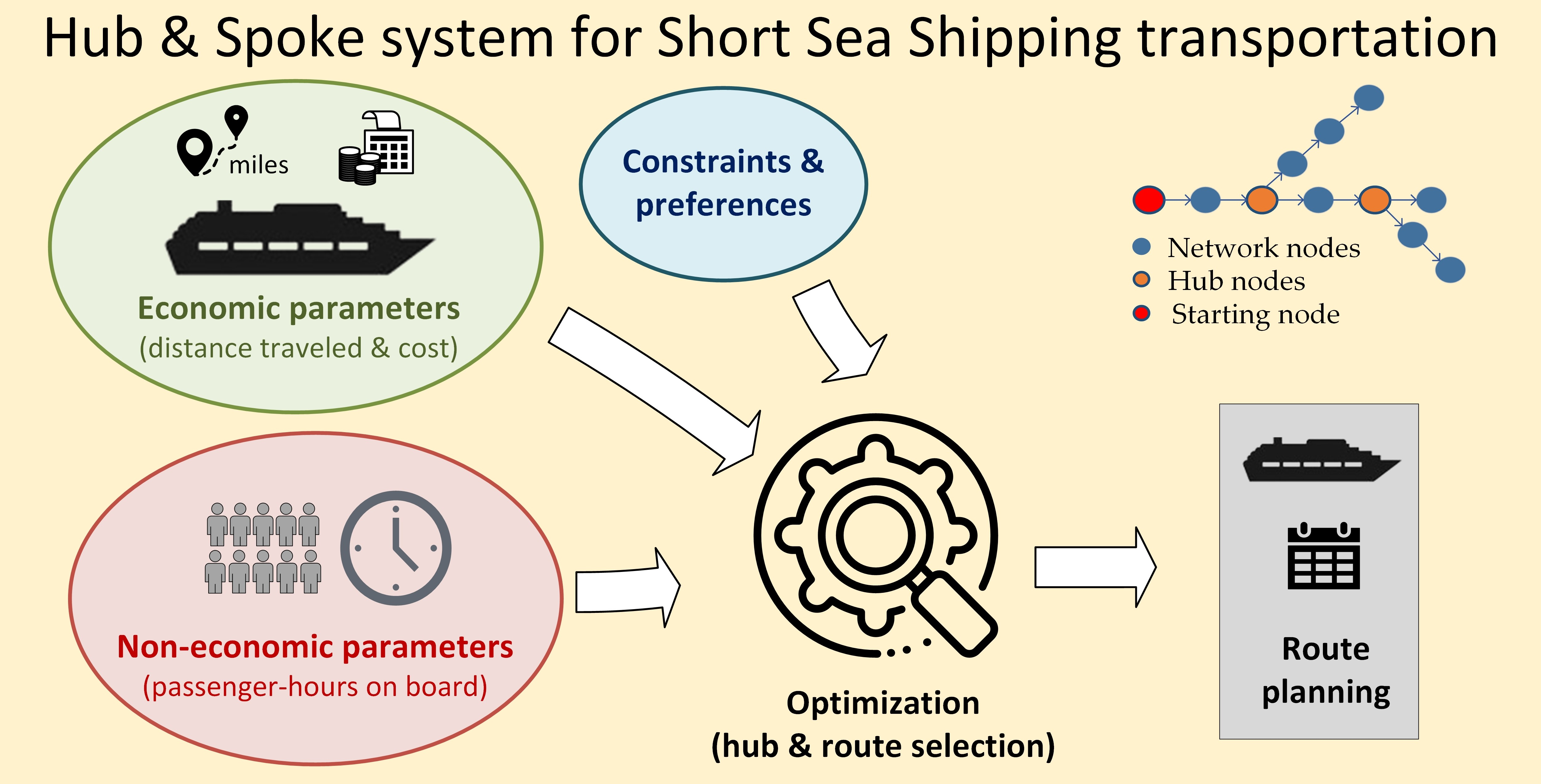
This research aims to develop an optimization methodology and design an H&S transportation system to regulate passenger flows within a cluster of quite sparsely located islands (or any other similar kinds of transport terminals) with a small number of carriages. In such types of problems, the passenger flows typically initiate from central ferry terminals, placed on the mainland, and distributed to the cluster islands. Such clusters involve mostly small-sized islands or tourist destinations; thus, the problem emphasizes passenger flows rather than vehicle and cargo transport. In these cases, it is not efficient to interconnect all islands directly to central ports. Instead, it is preferable to transfer passengers to a central node of the cluster (hub island) and then split the flows by routing additional lines (usually lower capacity and speed vessels) to different destinations in order to reduce carrier costs and passenger travel times. This problem structure differentiates from the typical H&S problem (
Figure 1), as islands are not directly connected to hub nodes. However, the algorithmic structure and computational approach fall within the same class of problems.
Short Sea Shipping transportation in a scatterly distributed islands constitutes a multi-parameter optimization problem in which decisions should be made regarding the number of vessels deployed, the hub selection, the route development, and the island service priority, subject to certain constraints and preferences. SSS is mainly adapted to the passenger movement particularities of scatter-distributed island regions, such as the Caribbean, Indonesia, the Baltic Sea, etc. Such an SSS network involves short irregular-shaped routes with several intermediate stops prioritizing popular destinations. This network development is similar in principle but different in application from the corresponding one for Artic waterways, which refers mainly to liner shipping networks involving long-distance and rather linear routes within limited navigable waters due to ice.
In this problem formulation, one or more main lines originate from the central ports and reach hub node islands where passengers may either continue their journey or transfer to other vessels toward their destination. The optimization model that is developed aims to provide proposals referring to the following:
the islands that are assigned as hub nodes within several potential alternatives;
the islands that are to be served by each route (vessel) originating either at a central port or at a hub node;
the island service priority within each route.
The problem formulation contains elements of the Hub-and-Spoke and Travelling Salesman structures, making it more demanding than the typical H&S one, as the hub selection within nodes and the shortest routes among islands are internal optimization goals. Considering, in addition, that the passenger flows change along route nodes, the use of formal optimization seems rather imperative to provide efficient routing solutions.
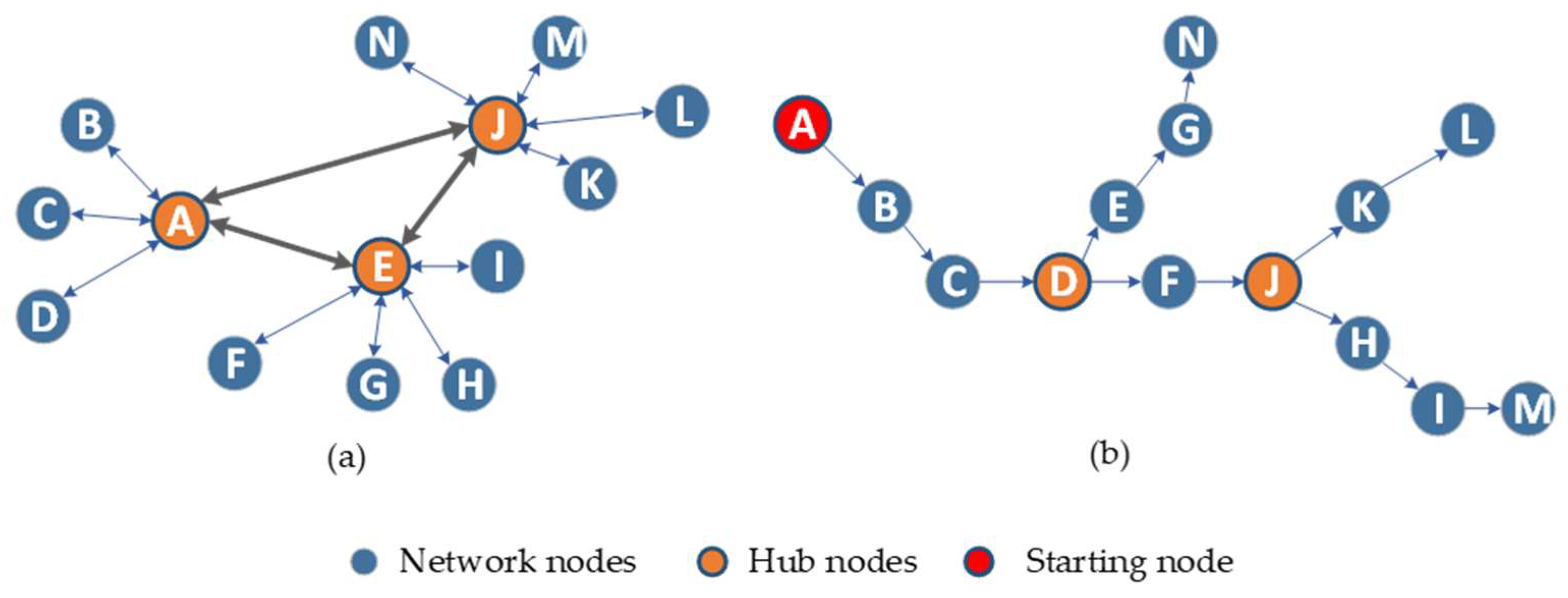
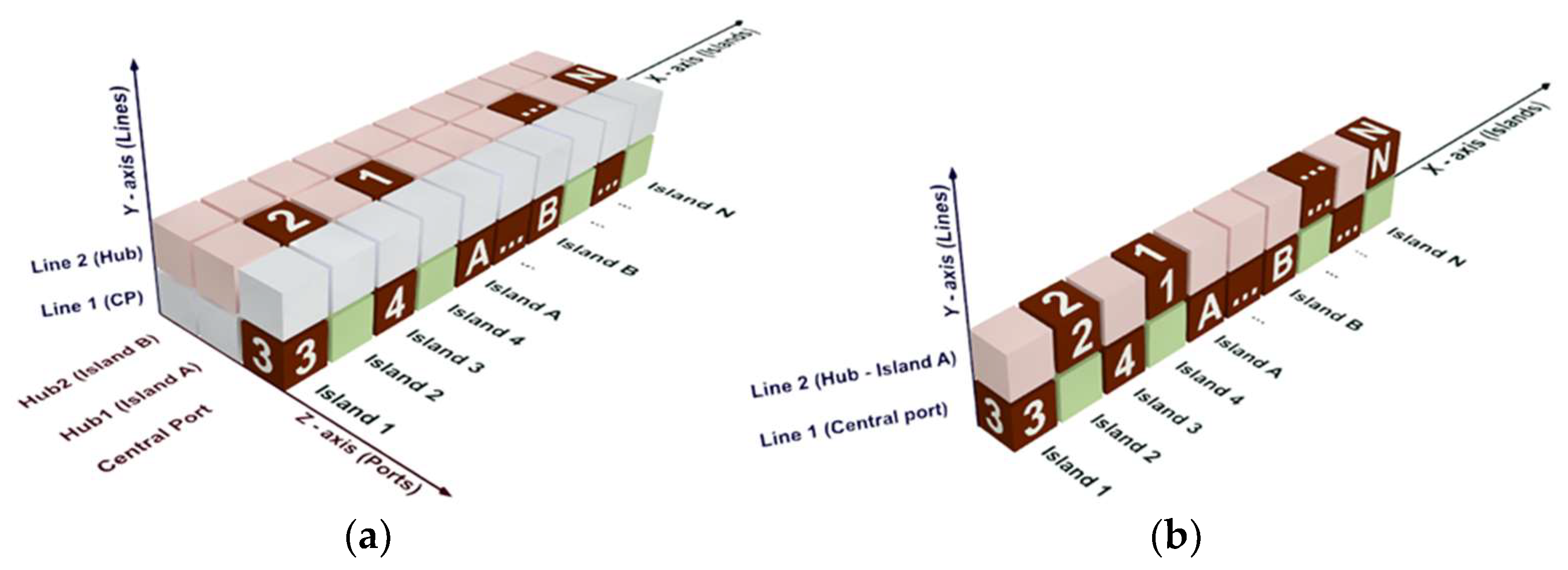
A 3-D tensor is employed to represent the solution structure for the proposed H&S model (
Figure 2a). In this formulation, the number of blocks along the X-axis indicates the islands to be served, while the number of blocks along the Y and Z axes reflects the number of lines (vessels) and the ports—potential origins (central ports or hub nodes), respectively. If the number of ports involved is equal to the number of lines (vessels), the problem is downgraded to a two-dimensional problem (island-to-line allocation and prioritization), and each solution can be represented by a 2-D permutation matrix, as shown in
Figure 2b.
A number of tensor blocks (as many as the islands) are numbered with a sequence of integers indicating the order of island service, and all others have no value. Every block set in the Y–Z plane corresponds to an island, and assuming each island is visited once, only one block is numbered. The numbered blocks are distributed in a series of block strings along the X–Z plane, indicating the islands to be served by each line.
Figure 2a depicts a representative solution for the H&S routing problem where two lines, one departing from the central port (Line 1) and one from a hub node (Line 2), are employed to serve a number of islands. The main port is predefined, while the hub node can be selected between two alternatives (A or B) among the islands. In this solution, the vessel employed for Line 1 departs from the central port and consecutively sails through islands 3, 4, A, …, B, … (with the potential hubs to be included). As island A is selected as the hub, the second vessel is routed from there, and passengers with final destinations islands 2, 1 …, and N transfer to Line 2 to complete their journey.
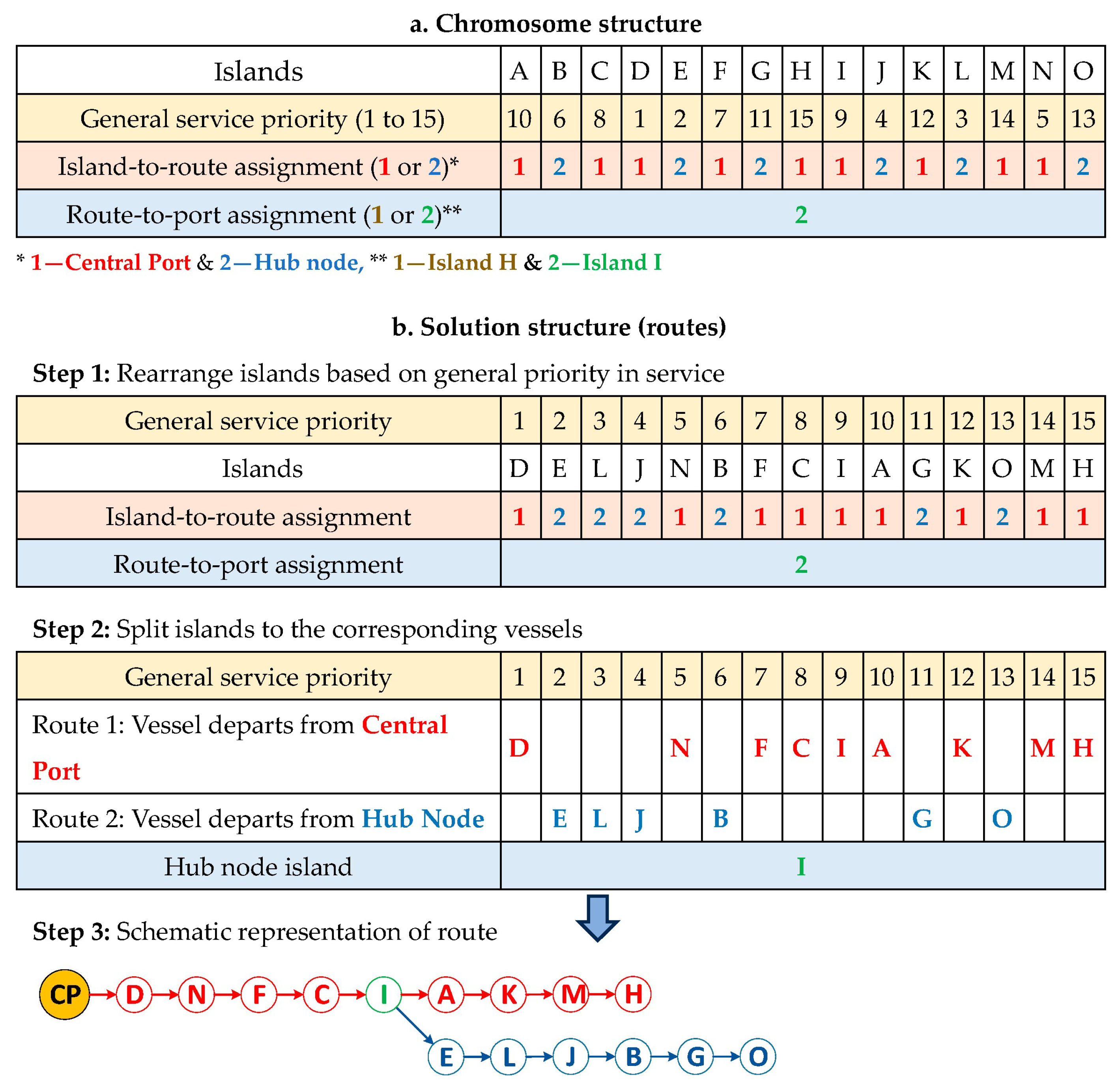
To further explain the chromosome (solution structure), an example is provided with reference to
Figure 3. The solution includes the general service priority of islands, the line by which each island is served and the hub(s) island(s). In this example, a cluster of fifteen islands (A to O) is considered to be served either directly from the central port or by transferring to a second vessel originating from a hub established in one of two alternatives (islands H and I). The “general service priority” part of the solution consists of fifteen unique integers (1–15) indicating the whole service priority of islands (
Figure 3a). The values in the next row mark the vessel line that will serve each island (1 and 2 correspond to vessels departing from the central port and the hub node, respectively). The value in the last assigns the hub node island to one among the predefined alternatives (Island I). Based on this information, the algorithm uses the general service priority to arrange islands to vessels and develop the service priority within separate lines (
Figure 3b).
4. Proposed Model
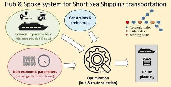
The proposed multi-objective tri-level optimization algorithm considers vessel-related cost parameters (transportation cost, also called ‘economic’ parameters) and user-related impacts, mainly referring to passenger journey times. Vessel costs are primarily related to traveling distances, while user impacts accumulate the time spent on board or during vessel transferring for all passengers. The optimization model further includes constraints resulting from operational limitations, such as the capability of a port to be used as a hub, the necessary times for embarkation–disembarkation, and vessel transfer. The model can additionally handle planning preferences for avoiding inefficient solutions/schedules, e.g., short vessel routes or long-lasting passenger trips.
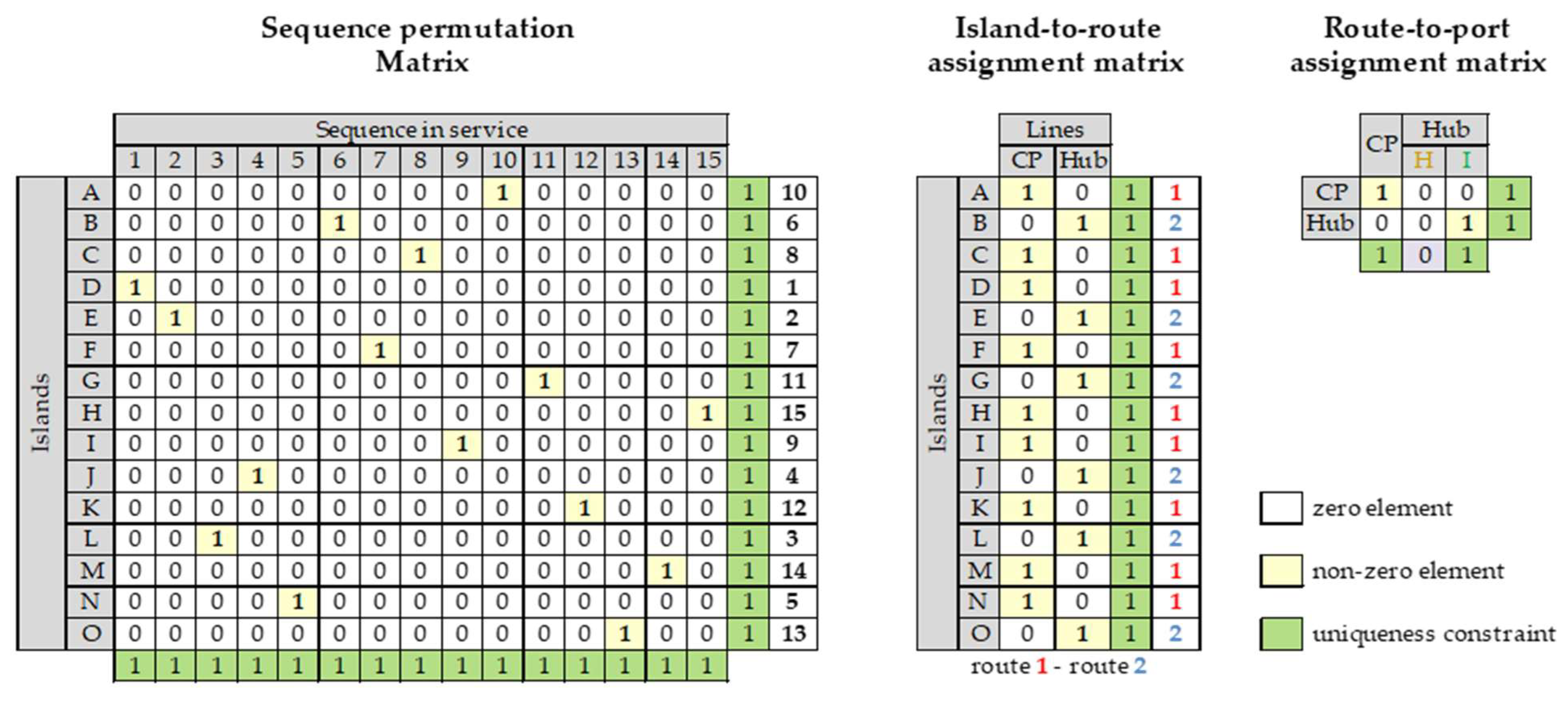
Matrix algebra is employed to structure the mathematical representation of the problem. In particular, three permutation matrices are developed (
Figure 4). The first is a square binary doubly stochastic matrix (with exactly one entry of 1 in each row and column and zeros elsewhere) for the one-to-one correlation of islands and general service priority. The second matrix is an orthogonal binary stochastic one (with exactly one entry of one in each row and zeros elsewhere) for assigning islands to the available routes, while the third is an orthogonal stochastic one (with the sum of all entries to be equal to 1 in each row and equal or less than 1 in each column) for assigning each vessel route to one of the alternative ports. Based on these initial matrices, which represent a solution, the algorithm initially rearranges the given input data to develop corresponding matrices with the physical island service sequence in each line (
Figure 3b). After that, it calculates the necessary output (e.g., arrival times, distances, passenger hours) for each node and link of the network and, finally, the fitness value for the whole network.
4.1. Model Assumptions
The Hub-and-Spoke model for Short Sea Shipment transportation considered in this study is described in detail with the following characteristics:
All passengers initiate their trips from a central port on the mainland.
Two types of routes are considered, direct connection from a central port or transit travel through a hub node connection.
Hub islands are served directly from a central port.
All islands are served once.
Several alternatives for placing hub nodes can be considered.
Ships serving different routes can have different velocities.
Time-varied intermediate stops are considered.
The generalized objective function evaluates the fitness of each solution (hub node selection and line routing) in terms of a weighted sum of economic and non-economic components as follows:
where D represents the total distance traveled by all vessels, PH is the total passenger hours spent in all journeys, and P represents any desirable preferences, while w
1, w
2, and w
3 are weight coefficients of the sub-objective functions. The first component closely relates to the traveling cost, while the second considers the number of passengers by destination, the average vessel speed, and the necessary time interval for passenger boarding and disembarking. These components are calculated as follows:
4.2. Parameters
| I | set of islands to be served |
| i | island index of an initial (random) island list, ∀ i ∈ {1, 2, …, I} |
| j | island index associated with the island service sequence, ∀ j ∈ {1, 2, …, I} |
| K | set of routes (lines) |
| k | route (line) index, k ∈ {1, 2, …, K} |
| L | set of alternative ports for route initiation (L ≥ K) |
| l | port index of route initiation, l ∈ {1, 2, …, L} |
4.3. Data
| vessel speed of journey initiating at port l, ∀ l ∈ {1, 2, …, L} |
| X coordinate of the port where vessel l initiates, ∀ l ∈ {1, 2, …, L} |
| Y coordinate of the port where vessel l initiates, ∀ l ∈ {1, 2, …, L} |
| number of passengers disembarking in island I, ∀ i ∈ {1, 2, …, I} |
| passenger transfer time in island I, ∀ i ∈ {1, 2, …, I} |
| X coordinate of island i port, ∀ I ∈ {1, 2, …, I} |
| Y coordinate of island i port, ∀ i ∈ {1, 2, …, I} |
4.4. Decision Variables
| sequence permutation matrix for assigning island i to priority sequence j, ∀ i, j ∈ {1, 2, …, I} |
| island-to-route assignment matrix for assigning island i to route k, ∀ i ∈ {1, 2, …, I}, k ∈ {1, 2, …, K} |
| route-to-origin node assignment matrix for assigning route k at initiation node l, ∀ k ∈ {1, 2, …, K}, l ∈ {1, 2, …, L} |
Equations (2)–(4) refer to the sequence permutation matrix ensuring that each vessel occupies a unique position in service priority order, (5) and (6) are related to the island-to-route assignment matrix allocating each vessel to exactly one route, and (7)–(9) are associated with route-to-port assignment matrix ensuring that each route is mapped to exactly one initiation node. If the number of routes is lower than the number of potential initiation nodes, some nodes will not be engaged, and relationship (9) holds as an inequality.
The following calculations aim to rearrange the rows of matrices and arrays described above based on the island service sequence that are associated with the specific chromosome/solution examined and, furthermore, assign islands and passengers to routes. Due to this row rearrangement, the previously employed index i becomes now index j.
The above calculations generate new matrices representing the routing matrix (10) and the corresponding to each route passenger matrix (11).
4.5. Auxiliary Matrix
| Island-to-Hub Node Assignment Matrix for assigning island i as hub node of route k, ∀ i ∈ {1, 2, …, I}, k ∈ {1, 2, …, K} |
4.6. Calculations
4.6.1. Distances
|
| the distance traveled between successive islands j − 1 and j of the vessel journey originating at port l, ∀ j ∈ {1, 2, …, I}, ∀ l ∈ {1, 2, …, L} |
4.6.2. Passenger Hours
|
| the cumulative distance of the vessel journey originating at port l up to island j, ∀ j ∈ {1, 2, …, I}, ∀ l ∈ {1, 2, …, L} |
|
| the travel time between successive islands j − 1 and j of the vessel journey originating at port l, ∀ j ∈ {1, 2, …, I}, ∀ l ∈ {1, 2, …, L}. |
|
| the arrival time at hub node connection l of vessel journey originating at a central port, ∀ l ∈ {1, 2, …, L} |
|
| the arrival time at port j of the vessel journey departing from node port l, ∀ j ∈ {1, 2, …, I}, ∀ l ∈ {1, 2, …, L} |
|
| the departure time from port j of the vessel journey originating at port l, ∀ j ∈ {1, 2, …, I}, ∀ l ∈ {1, 2, …, L} |
|
| the passenger hours spent on board by passengers in vessel departing from port l and disembarking at island j, ∀ j ∈ {1, 2, …, I},∀ l ∈ {1, 2, …, L} |
where
is the arrival time of vessel departing from a central port to island i and
in the case that island i is assigned as the hub node l.
4.7. Constraints and Preferences
Several constraints and preferences can be incorporated into the model to simulate some realistic aspects of the problem. The most important are:
the travel time of each vessel does not exceed a specified value;
the passenger travel time does not exceed a specified value;
the service time of a particular island does not exceed a specified value;
a desired priority for serving a particular island can be set;
a specific island may be served directly from the central port;
a minimum and/or maximum number of islands served by a single vessel can be set;
constraints regarding islands’ (operational) capability to serve as hub nodes can be set.
4.8. Model Structure
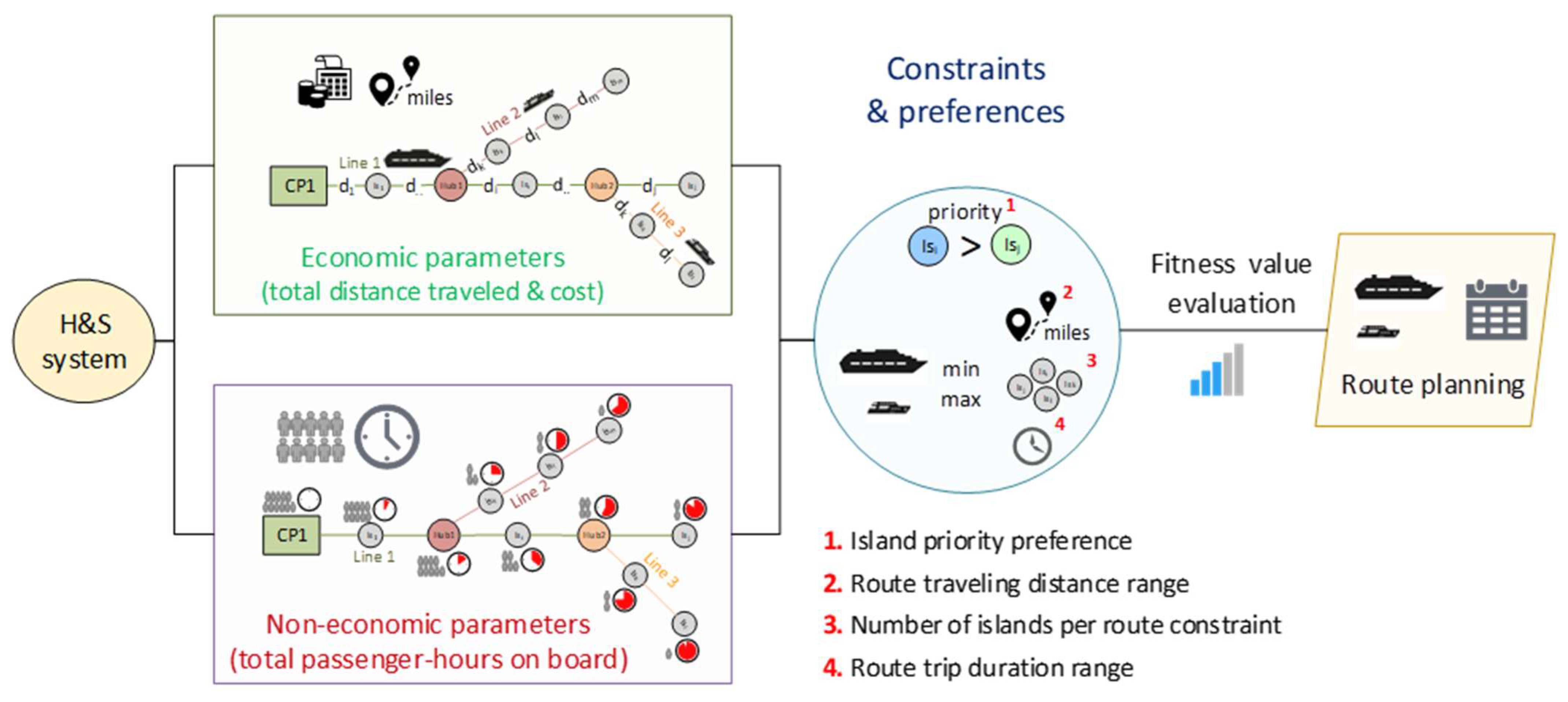
Figure 5 graphically illustrates the optimization model structure. The fitness value is computed for the specific route plan based on the routes developed by a candidate solution and the constraints and preferences adopted. In particular, the total carrier cost, resulting from traveling distances of individual routes and unit costs, is calculated as the economic component of the problem. Further, the total number of passenger hours in all routes is accumulated to develop the second part of the objective function. These two parameters are appropriately tuned (based on the maximum value found running the algorithm as a single objective) depending on the desirable impact of each one on the objective function. All the examined solutions undergo constraint and preference satisfaction checks before they are compared to each other to develop the optimal routing plan. Indicative (hard) constraints and (soft) preferences include the island service priority, upper and lower bounds for vessel traveling distance or number of served islands, maximum allowable journey time for passengers, avoiding long- or short-lasting trips and giving service priority to more popular destinations. Model economic and non-economic parameters are fine-tuned following normalization based on their mean values before applying the weighting process.
The H&S network design problem is a complex combinatorial optimization problem and belongs to the NP-hard class of problems, which means that the problem complexity and the computational resource requirements grow significantly as the numbers of nodes and constraints increase. Genetic algorithms (GAs) have been extensively used in recent years to solve large and complex combinatorial optimization problems due to their capability to provide acceptable (near-optimal) solutions within a reasonable computational time for typical problem cases.
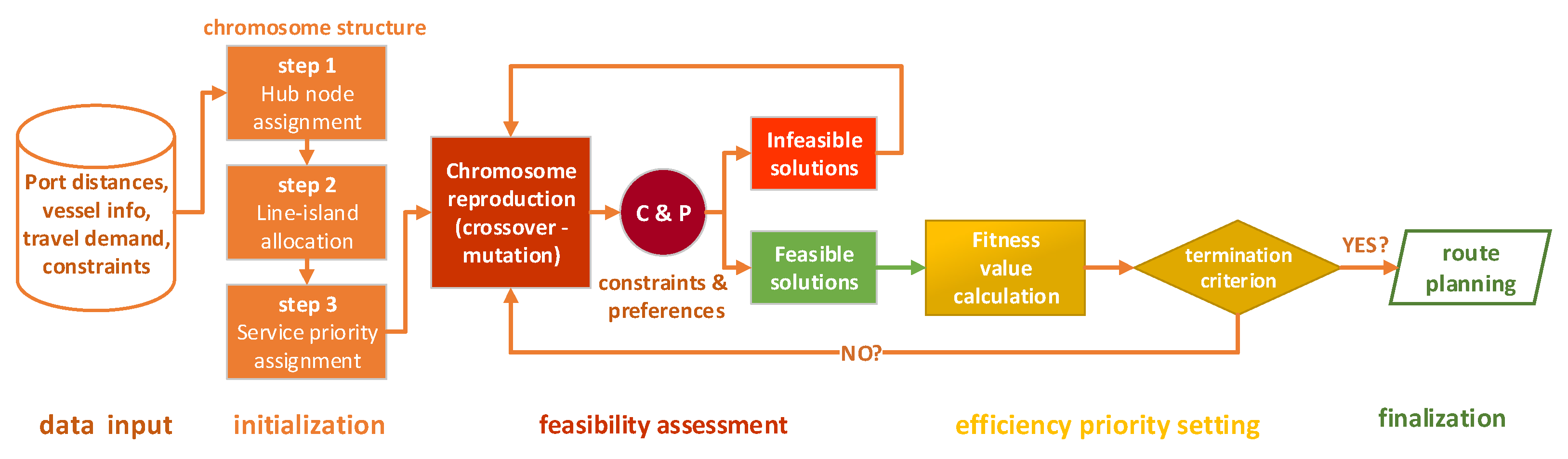
Figure 6 schematically depicts the optimization structure and methodology. The system is initially fed with all necessary inputs, such as island distances, vessel speeds and unit costs, the number of passengers per destination, etc. Following the typical GA evolutionary process, the algorithm develops a population of initial solutions using random values to optimize the three fundamental parameters, i.e., hub node selection, island assignment to vessels, and island service priority. Individual solutions undergo reproduction through crossover and mutation operations within the population, and new solutions are generated. The solutions are initially checked for validity (constraint and preference fulfillment) and then evaluated in terms of their fitness value. The process terminates when a predefined number of iterations are made without considerably improving the fitness score.
More specifically, the genetic algorithm is parameterized with a 50-chromosome initial population with the crossover and mutation rates being 0.5 and 0.1, respectively, in all test cases and following a relevant analysis. The termination criterion involves the performance of 20,000 trials without substantial improvement (less than 0.01%) of the fitness value. The problem has been built in the MS Excel environment for easiness in data handling and model implementation. Optimization is performed using the commercial GA software Evolver v8.4.0 of the Palisade Company (now named Lumivero), which runs as an Excel add-in component.
5. Case Study Applications
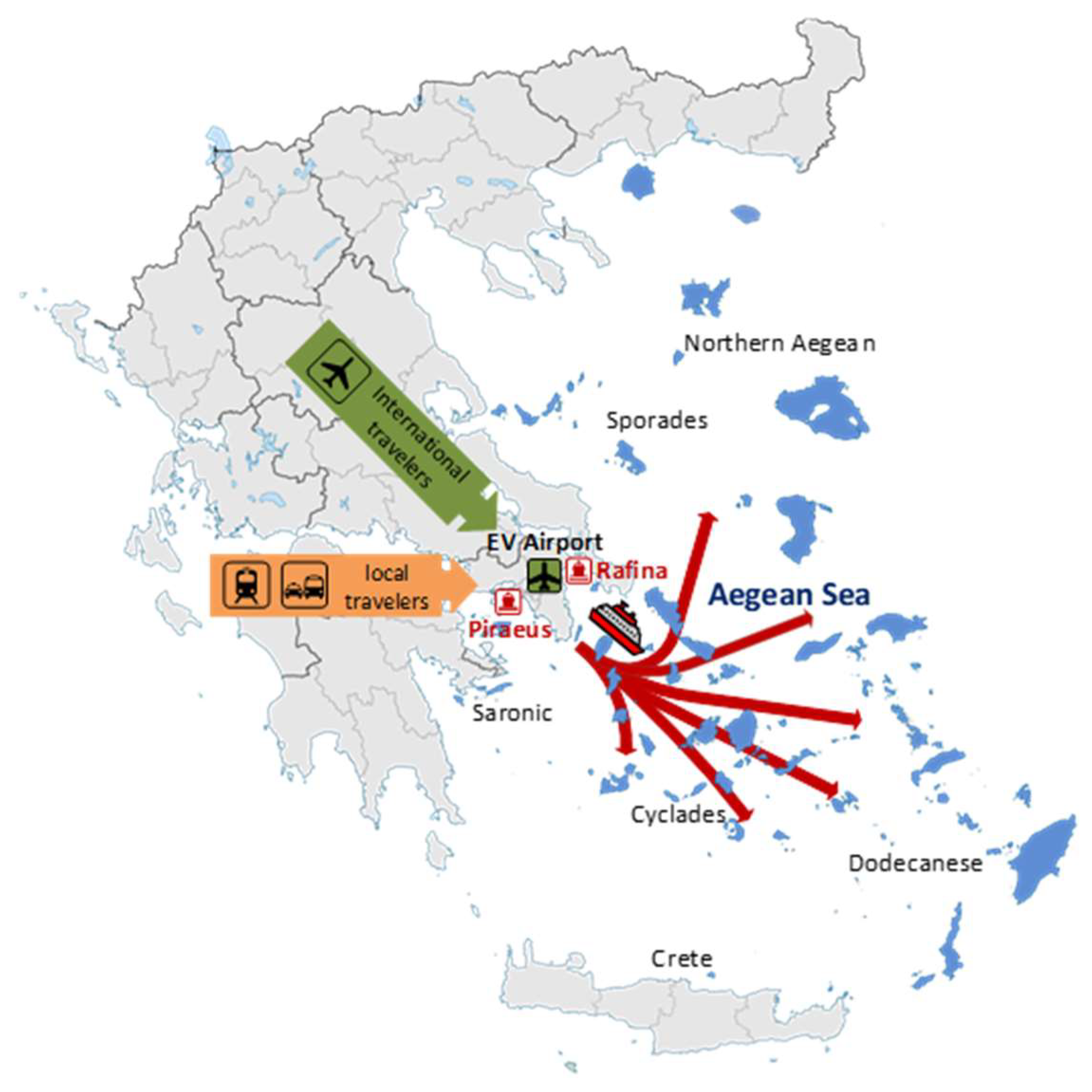
Two case studies have been developed to analyze and evaluate the proposed H&S transportation system’s effectiveness in regulating vessel routes and passenger flows moving from mainland Greece to the Aegean Islands. The first includes 17 ports, and the second includes 51 ones. The Aegean Islands cluster includes more than 150 inhabited islands, many of them being within the top tourist attraction destinations. Two central ports on the mainland (Piraeus and Rafina, next to Athens) connect to the Aegean Islands, serving more than 3 million visitors yearly. Piraeus Port (one of the busiest ports in the Mediterranean and Europe) is located 12 km southwest of Athens and constitutes the Aegean Islands central getaway. Rafina is located 50 km northeast of Athens, is the second gateway port for the Aegean Islands, and has presented significant growth in recent years.
Figure 7 presents the location of the two central ports and the traveling flows to the Aegean Sea islands.
Several cases and operational scenarios have been developed for model testing and evaluation based on the Network of Short Sea Shipping in the Aegean area. The island cluster that is considered in the case study consists of 15 islands, rather sparsely and unevenly located on the map to facilitate result justification.
Table 1 illustrates the necessary data for the case study application. They include the distances between islands, the number of passengers by destination, and the vessel’s average speed. The time for boarding and disembarkation is assumed to be ten minutes on every island.
Vessels can depart from two central ports (Piraeus or Rafina), while three islands (Chios, Limnos, Ikaria) have been set as potential Hub nodes. Two vessel types with different characteristics (speed) are considered depending on their route origin. The following scenarios are examined to evaluate the model’s capability to effectively and realistically assess optimal route planning:
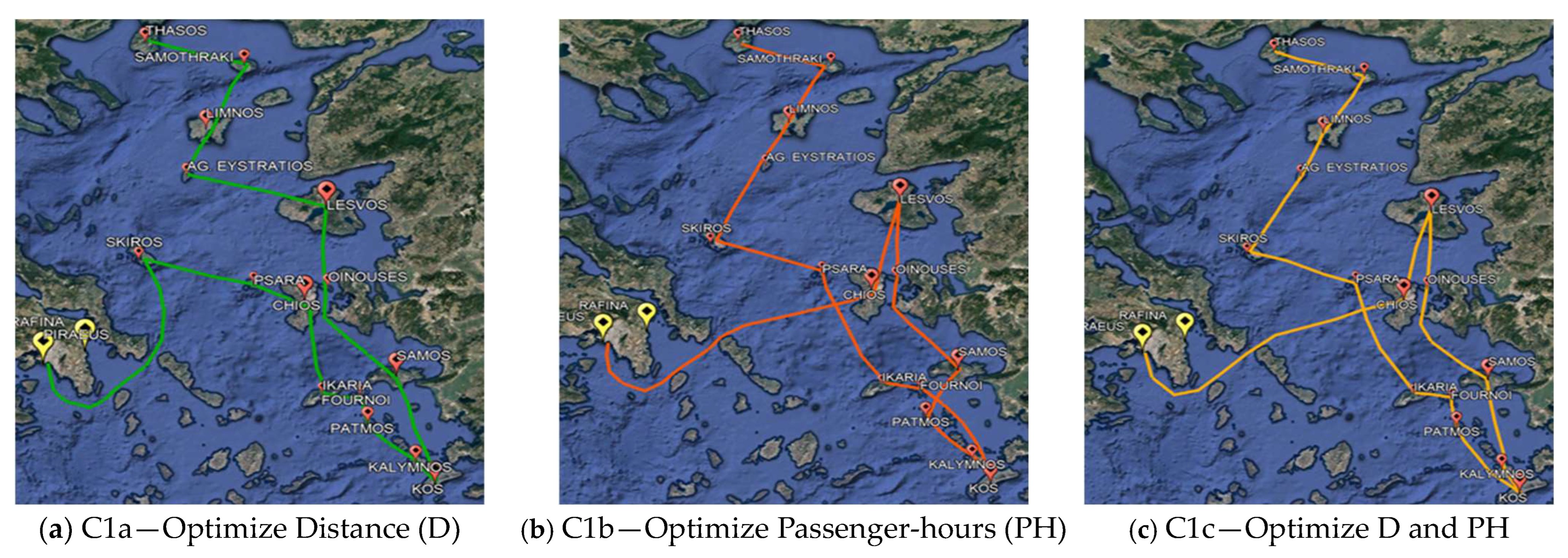
C1: One vessel departs from a central port (Piraeus) and serves all islands without hub nodes.
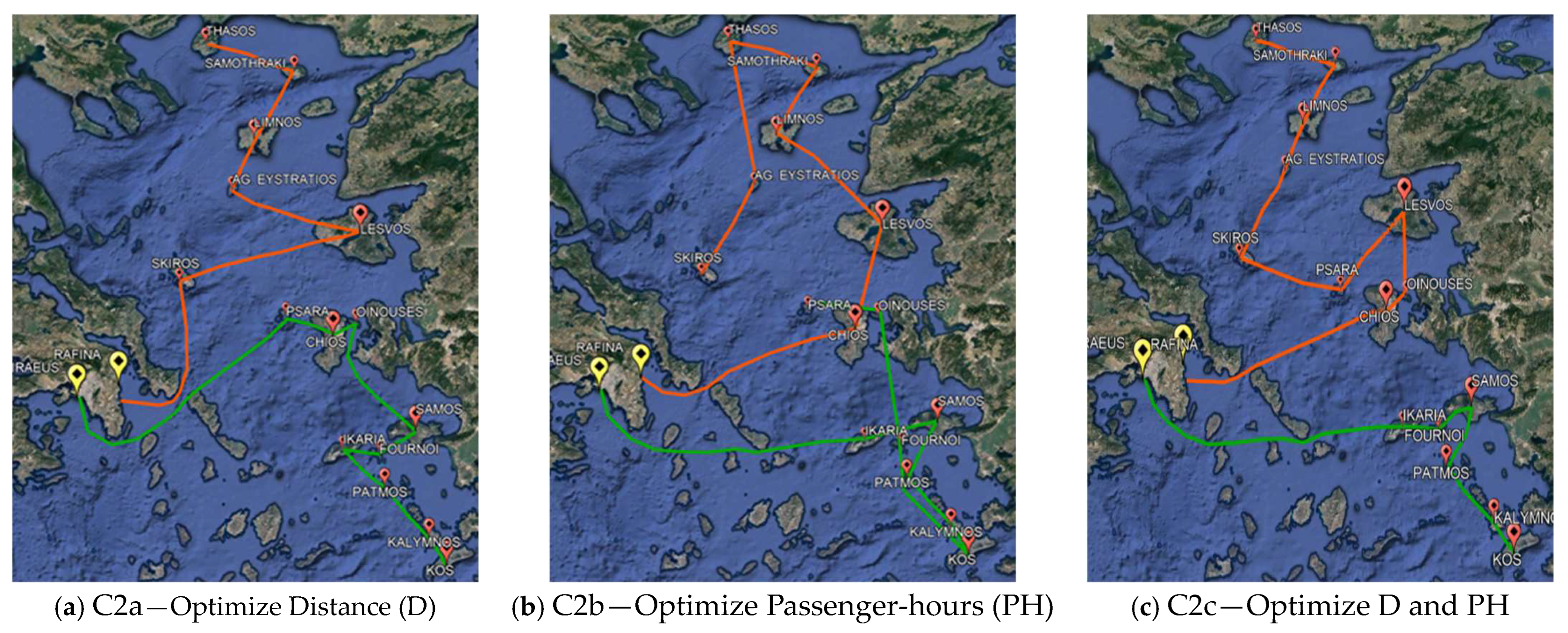
C2: Two vessels depart from central ports (one from Piraeus and one from Rafina) and serve all islands without hub nodes.
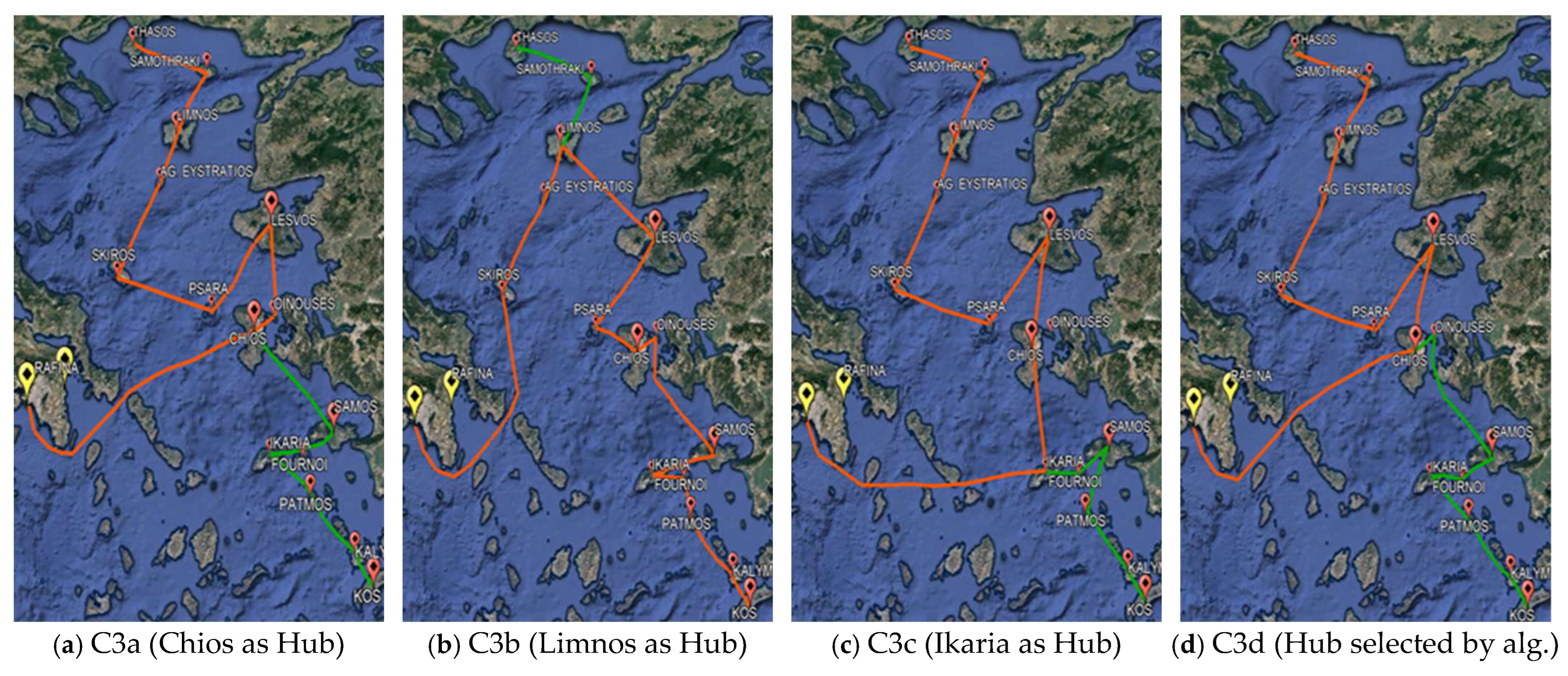
C3: One vessel departs from a central port (Piraeus) with one hub connector.
C4: Two vessels depart from central ports (Piraeus and Rafina) with one hub connector to be assigned by the algorithm.
The optimization is performed upon single or combined objectives referring to the total distance traveled (D) and the cumulative passenger hours (PH) while two more parameters are recorded and evaluated in each case, the total travel time (T) of all vessels and the maximum trip length (Tmax-trip) among all passengers.
The simplest case, C1, where one vessel serves all islands, imitates the classic Travel Salesman Problem (TSP). Three alternatives are presented to emphasize the scope of the proposed methodology. C1a aims to minimize the traveling distance (and consequently the routing cost). C1b attempts to reduce the total passenger time spent on board. C1c provides a trade-off solution between the above (into some extent) competing goals. The results in
Figure 8 indicate that C1a provides the shortest route but at a considerable expense of the total passenger time on board. InsteadC1b recommends a relatively lower total passenger time solution compared to C1a but with increased traveling distance. This happens because small islands with fewer passengers are left to be served last without special attention to proximity criteria. Further, several alternative solutions can be found following the trade-off between the two goals. An indicative such solution (C1c) achieves an almost minimum passenger-hour solution and a competitive traveling distance one.
In Case 2, two vessels depart from central ports (one from Pireaus and one from Rafina) to serve the whole island cluster. As anticipated, the proposed solutions in every case develop the routes in geographically separated sub-regions (northern and southern islands). The results in
Figure 9 indicate that C2a provides the shortest vessel routes in total, C2b the minimum cumulative passenger-hour solution, and C2c a more comprehensive solution that aims to facilitate both objectives. In general, the latter solution achieves very competitive figures in total vessel traveling distance and time as well as in cumulative passenger time spent on board. Compared to case C1, the total distance has marginally been extended, but the passenger hours have been sizably cut down.
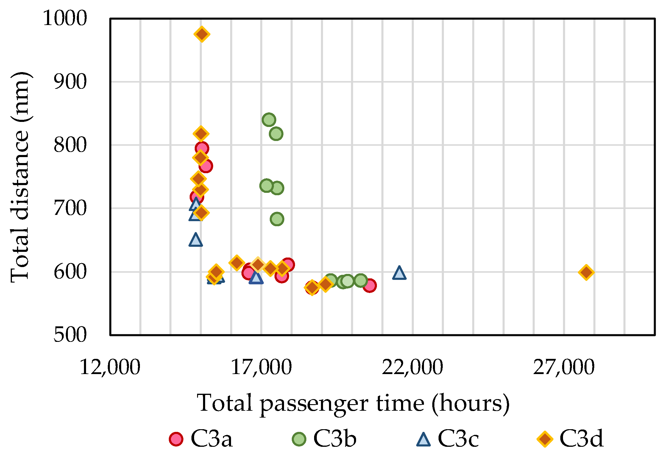
In scenario C3, one vessel departs from Piraeus central port and another from a hub node, the latter being alternatively set in one of three large islands (Chios, Limnos, or Ikaria) that can serve as hub connectors. Three solutions have been developed corresponding to each of the alternative connectors (C3a, C3b, C3c). A fourth case strives for an optimal solution by demanding the algorithm to automatically assign the hub node among the three islands (C3d). The evaluation is made upon trade-off solutions including the total vessel route distance (D) and the cumulative passenger time (PH), with indicative results presented in
Figure 10. All solutions present comparable traveling distance values (within a 4% deviation range), while C3c outperforms in terms of passenger time. This is because Ikaria is closer to Piraeus port and in the core of the islands with high travel demand. In C3d, the algorithm has selected Chios as a hub and provided a competitive solution even though the algorithm complexity rises significantly in the case that the algorithm needs to determine the hub-node location internally. This capability may be highly effective in large-scale problems or sparsely positioned island nodes. In the latter case, a full algorithm implementation can initially provide almost-best hub node selection, while a downgraded algorithm application (with known hubs) can provide improved routing solutions.
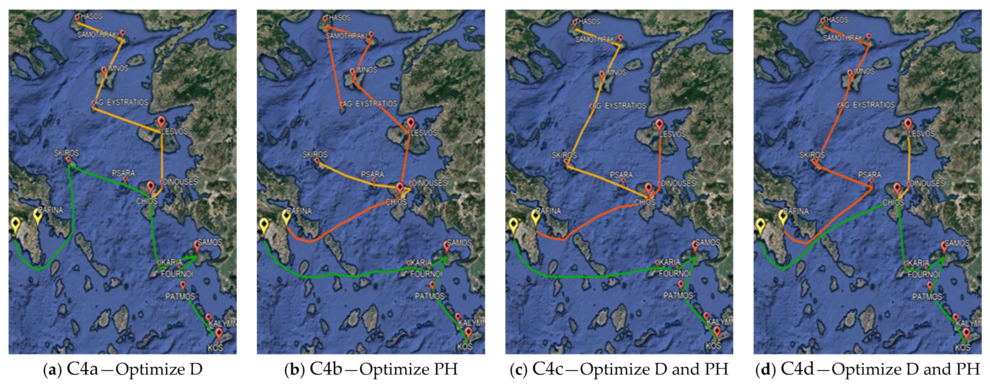
In a broader problem structure, case C4 considers up to two ships departing from central ports (Piraeus and Rafina) and one from a hub node to be assigned by the model among Chios, Limnos, or Ikaria islands. When optimizing the total traveling distance (C4a), the model proposes a solution involving one vessel from Piraeus Central Port, covering the southern part of the islands, and another from the hub node of Chios with a northern direction. Although reducing the total traveling distance, the employment of two vessels results in high passenger hours spent on board and extensive trip times. Optimizing the total passenger hours on board (C4b) leads to a three-vessel solution with almost half the total passenger and individual trip time (in comparison to C4a), at the expense, however, of the total traveling distance, which increases by a factor of approximately 25% (
Figure 11). The multi-objective approach (C4c) provides a balanced solution in terms of traveling distance and total passenger hours (with three vessels in operation). However, the generated solution is not entirely satisfactory in terms of the max trip time (26:16 h), which results from the fact that a slow-speed vessel has been assigned to serve the distant islands. To reduce this prolonged journey, a constraint is set in case C4d to avoid solutions that exceed a fifteen-hour trip limit. In such a case, the algorithm provides a quite different route planning solution that provides competitive performance values in regard to the main evaluation parameters but with a significant reduction in the maximum trip time. The comparison of the last two cases indicates that the problem holds a large solution space and that quite different routing solutions may lead to comparable fitness values demonstrating the potential of several local optima in such kinds of problems.
To gain a better insight into the multi-objective optimization outcomes, several iterations with varying sub-objective weights were conducted for case C3, and the results are depicted in
Figure 12. It is interesting to note that in every case, a well-shaped Pareto front is developed with a main characteristic that there is an almost sharp (rather than gradual) adjustment to the ultimately lowest level of each objective parameter. In fact, it appears that each Pareto curve closely fits into two straight lines, indicating the lowest total traveling distance and the lowest cumulative passenger time, respectively. Depending on the hub selection, these lines may be shifted at different levels of performance. For instance, selecting Limnos as the hub island (C3b), despite the efficiency concerning traveling distance, it cannot compete with other solutions in terms of total passenger hours spent on board. The reason is that the island is located well in the northern part of the cluster, and many passengers directed to the south have to make a wide deviation of the straight-line pathway. The automatic hub assignment in C3d has provided comparable results to those of the manual hub selection in the whole parameter range.
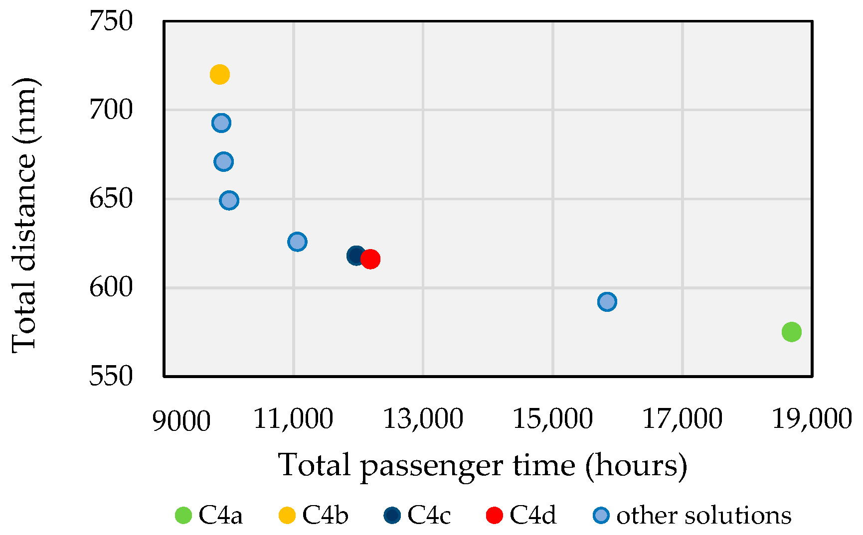
In case C4, when minimizing the traveling distance (C4a), the algorithm results in a solution with only two vessels in use and the passengers spending a significant amount of time on board. On the other end, minimizing the total passenger hours (C4b) leads to a rather extended traveling distance plan. Several solutions exist between these two extreme cases that follow the trade-off between the two objectives (
Figure 13), which can be developed by adjusting the relative weights in the objective function. A number of solutions almost retain the minimum distance value to the left of the diagram; however, beyond a point, an inclined and rather linear point pattern is developed along the Pareto front describing the relation between traveling distance and passenger hours. The developed solutions in C4c and C4d lie close to the turning point of the Pareto front. It is concluded then that a full weight-related sensitivity analysis is necessary to fully understand the solution’s effectiveness.
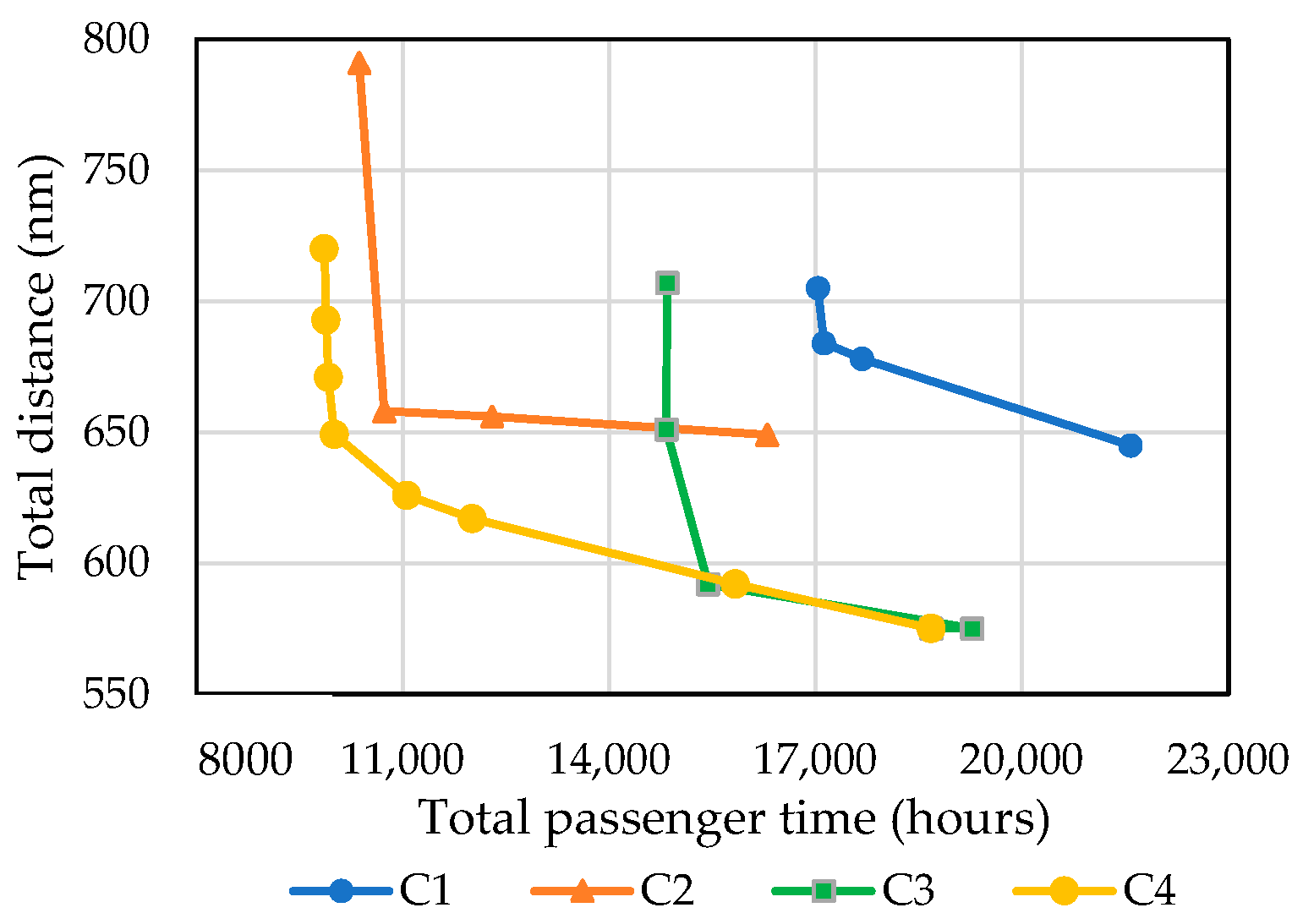
Figure 14 presents the Pareto curves developed after several runs of all scenarios examined in the case study. The results indicate that routing only one vessel from the central port to all island nodes (case C1) takes too long (in terms of both distance and time spent on board) to serve the whole cluster. Instead, routing two vessels originating from the central ports and without any intermediate hub (case C2) can better allocate island service with a significant impact on passenger cumulative time but not on the traveling distance. The introduction of a hub line along with a mainline from the central port (Case C3) leads to observably improved solutions (compared to those of C1) in terms of both decision parameters. Finally, the employment of additional vessels (case C4) can improve the effectiveness but not in all regards. In particular, the total passenger time is reduced but not the total distance traveled (compared to C3). In fact, if the goal is distance minimization, this can be equally well facilitated by a two- or three-vessel configuration. The decision, though on the appropriate number of vessels, does not solely rest on the optimization result but is also related to constraints regarding ship availability and capacity in conjunction with the travel demand.
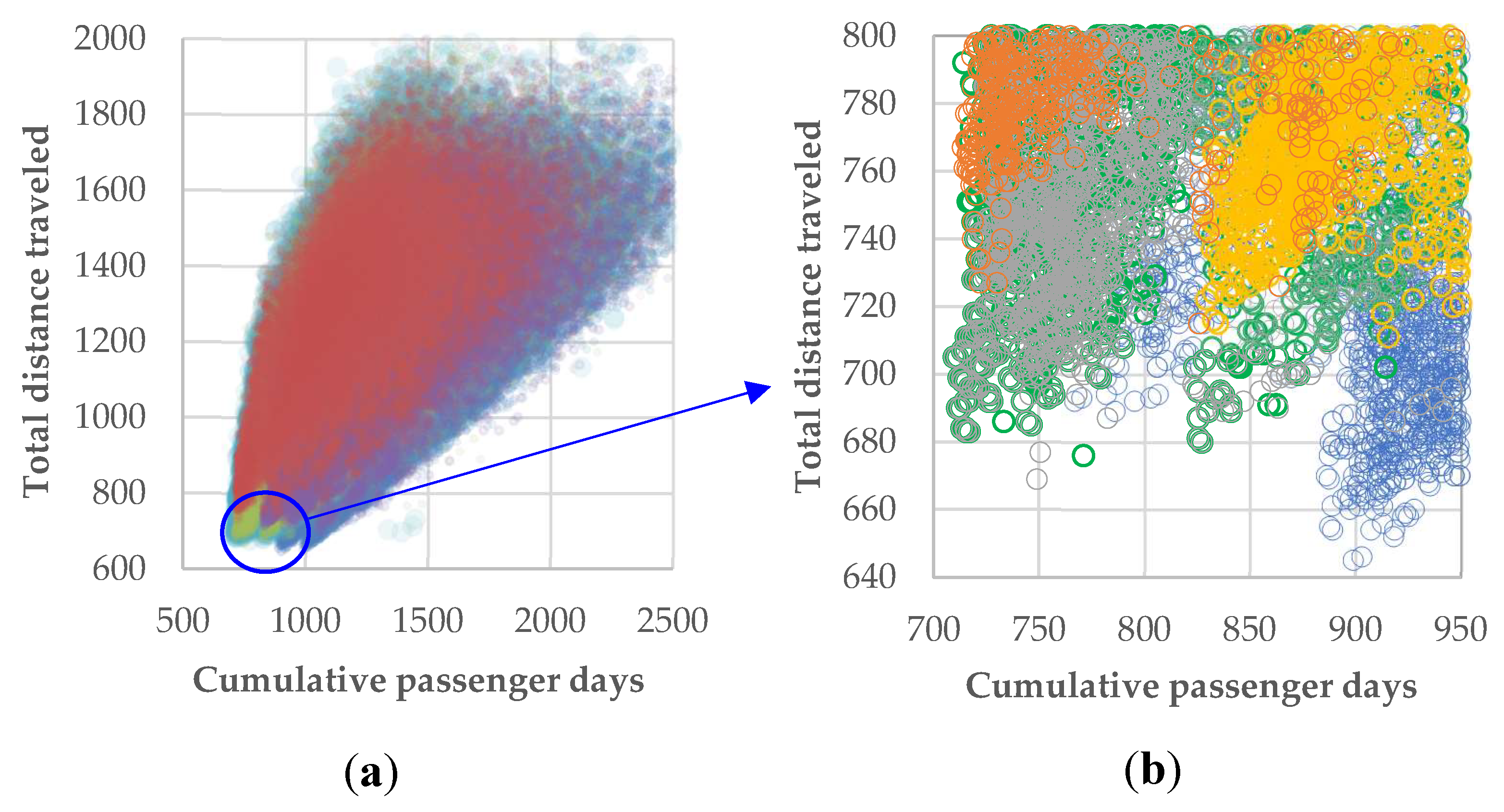
To obtain a wider picture of the solution space between the two main decision parameters (i.e., total distance traveled D and cumulative passenger hours PH),
Figure 14 presents the point clouds of all solutions from the execution of the algorithm at different levels of parameter weighting. Solving a particular weighting case study leads to a footprint-like point cloud between D and PH, indicating a roughly linear relationship between them. As the weights w
1 and w
2 of Equation (1) are altered (after scalarizing the two parameters), the produced point clouds are moved to an up-left and down-right direction (
Figure 15a). A full-range Pareto front is formed based on individual points corresponding to different decision parameter weighting (
Figure 15b).
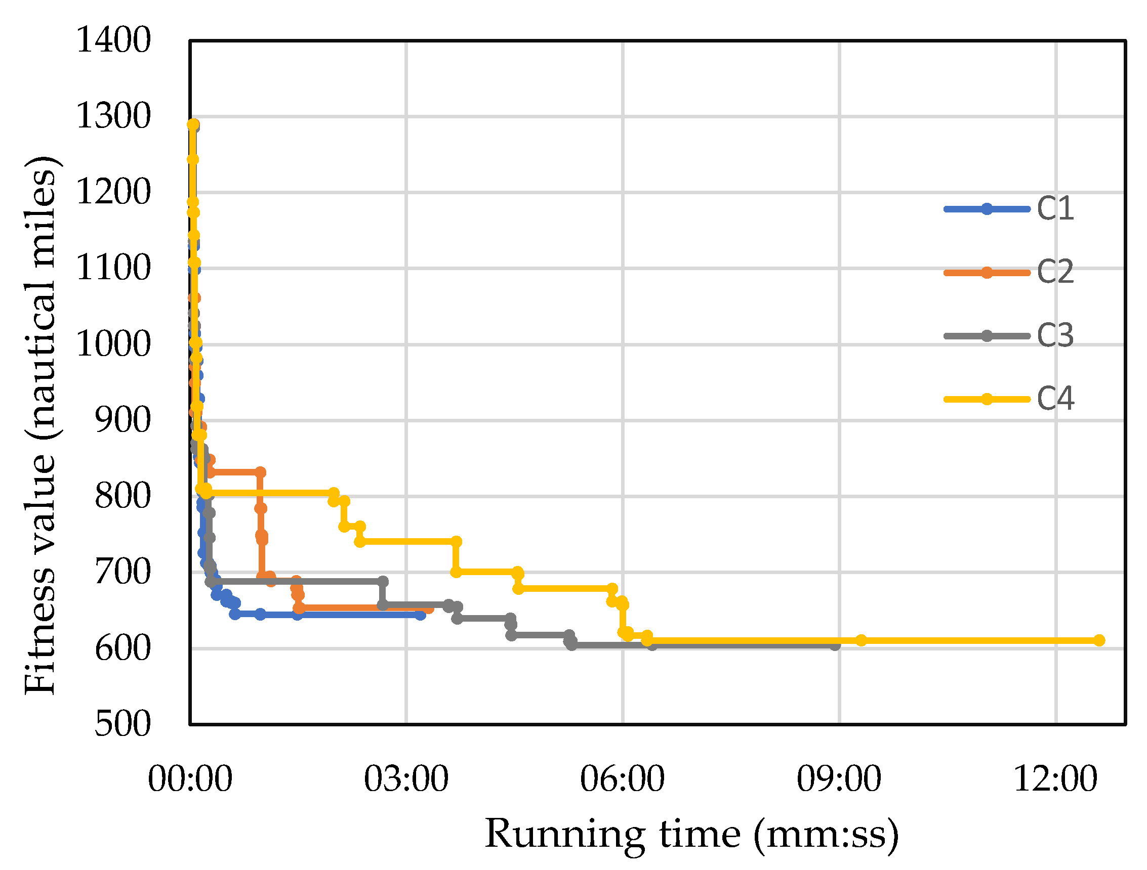
Regarding computational requirements, the time needed for algorithm convergence increases with the magnitude and complexity of the problem.
Figure 16 depicts the typical convergence curves for the four cases examined (C1 to C4). In general, the problem complexity increases with the number of vessels and the potential hub nodes. This is why the convergence speed drops from the simplest case (C1) to the most demanding one (C4). Accordingly, the convergence time in a PC with common characteristics (Intel
® Core ™ i7-7500, CPU 2.90 GHz, RAM 8.00 Gb) progressively increases and ranges from about a minute (case C1) up to seven minutes for the most demanding case (C4).
To examine the scalability of the proposed methodology, evaluating the Hub-and-Spoke modeling effect in SSS transportation and the algorithms’ robustness in providing efficient solutions for larger applications, an extension of the previous case study consisting of 49 ports of the same island cluster has been considered. The appropriate number of vessels for transferring passengers from the mainland to the cluster is four; thus, three alternative scenarios employing four, five and six vessels were tested. These scenarios are as follows:
C5: Four vessels depart from central ports (three from Piraeus and one from Rafina);
C6: Four vessels depart from central ports and one from a hub connector (selected by algorithm among several alternatives);
C7: Four vessels depart from central ports and two from hub connectors (selected by algorithm among several alternatives).
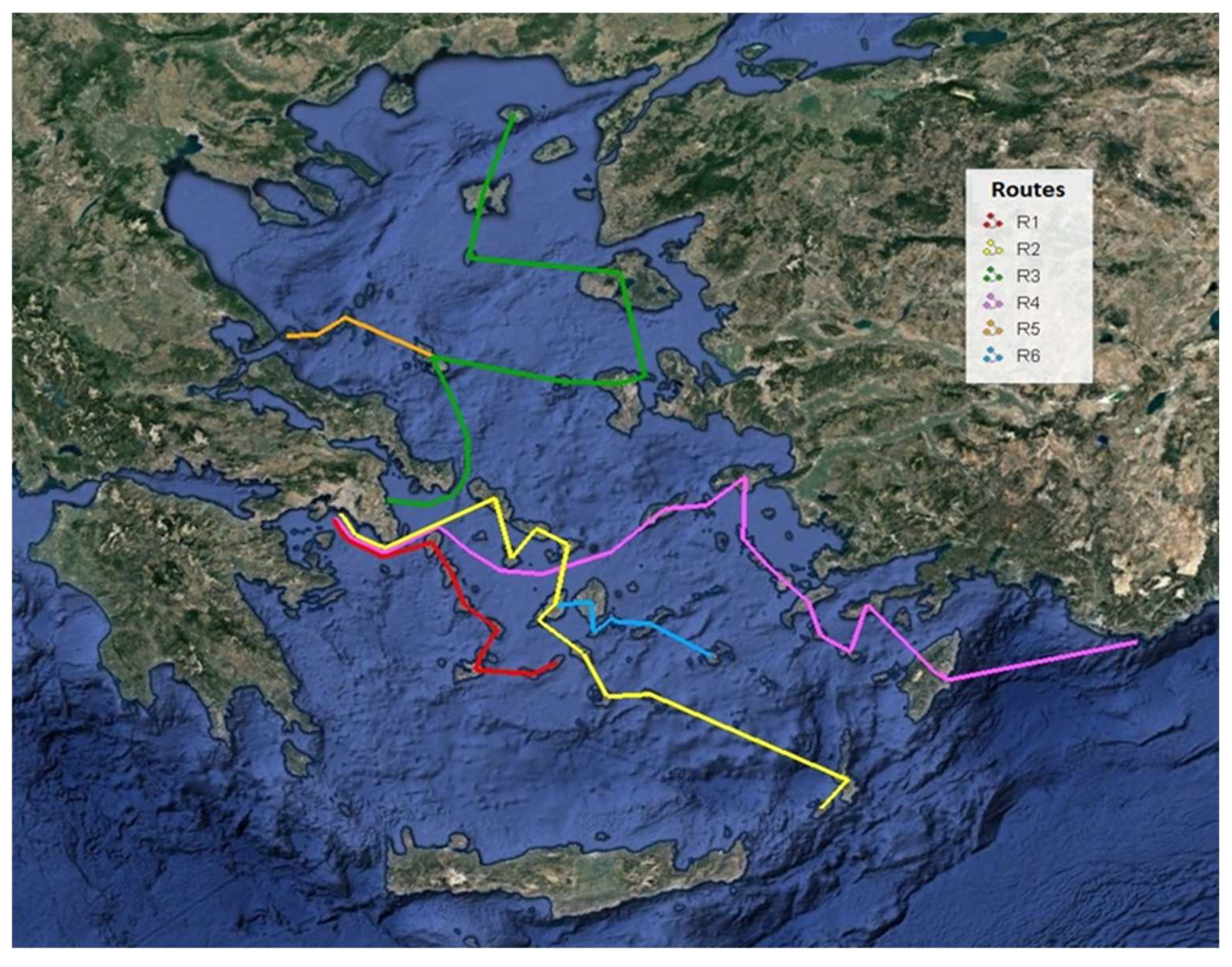
In case C5, the optimal traveling distance is 1666 nm while the optimal passenger hours is 26,347. Due to the limited number of vessels, the longest route facilitates 18 vessels. As the number of vessels increases, adding ferries from hub nodes (cases C6 and C7) decreases the traveling distance and passenger hours, resulting from the gradual split up of the flows after the passengers transfer deeply into the cluster. To avoid long-lasting trips, a constraint on the maximum number of intermediate stops is set at 20, 12, and 12 stops for cases C5, C6, and C7, respectively. From the results presented in
Table 2, it is concluded that by employing ferry boats from hub nodes, both the traveling distance and passenger hours decrease, providing a more comfortable journey to the passengers and reducing the traveling costs (fewer miles and partly involvement of smaller ferries with lower cost). An indicative travel plan for case C7b is schematically illustrated in
Figure 17.
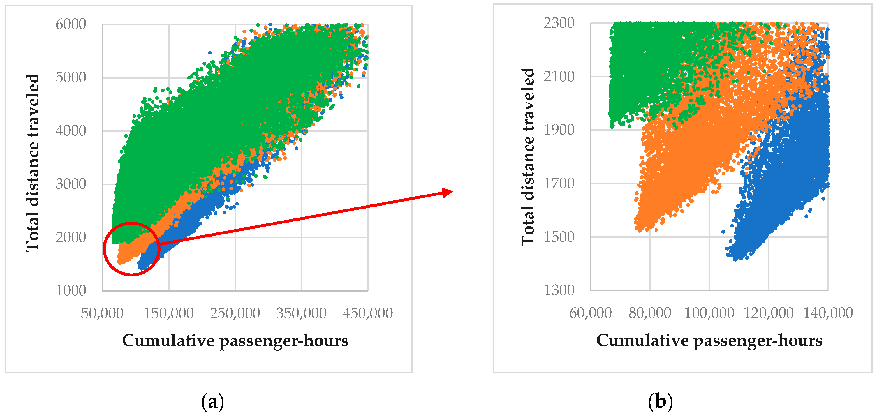
The selection of the appropriate number of vessels, in accordance with the number of islands and passengers served, is important in optimizing the set goals. Conversely, an ineffective solution may lead to a dramatic increase in the goal parameter values. To account for such discrepancies, the special case of one vessel, corresponding to the simple traveling salesman problem, is considered for the latter case of the 49 island cluster. The total distance is not much increased since, when several vessels depart from the central port, they travel in parallel for some distance before diverging to different directions. In contrast, the cumulative passenger hours on board are three to five times larger than those in
Table 2, as indicated in
Figure 18. In this extreme case, a trade-off analysis with different sub-goal weights results in notable solution deviations and a well-structured Pareto front. Indicatively, the total distance and passenger hours at the edges of the three point clouds of solutions, derived by different weights of the optimization sub-goals, are (1912–67,210), (1523–76,460), and (1415–108,710), respectively.
To further elaborate on the model effectiveness, three randomly generated instances (not related to the previous case study with actual islands) with a gradually increased degree of difficulty are tested to evaluate the algorithm performance in small-, medium-, and large-scale problems. The small instance includes 15 islands to be served by 2 lines (routes) that can be initiated from 3 alternative ports, the medium instance includes 50 islands and 6 lines that can be initiated from 8 ports, and the large instance includes 100 islands and 12 lines that can be initiated from 15 ports. The algorithm evaluation is performed at three distinct optimization objectives of minimizing the traveling distance (D), the passenger hours (PH), and the combination of them, respectively. Due to the stochastic process of the optimization search, three iterations for each scenario have been performed to provide an indication of the solution variability.
The results shown in
Table 3 indicate the algorithm’s robustness in solving small instances as, in all cases, the optimization results rapidly and closely converge to specific values. As the magnitude and complexity of the problem increase (medium and large-scale instances), although the solution quality in terms of convergence is slightly reduced, the algorithm remains capable of providing acceptable solutions. On the other hand, the required computational time is substantially increased and is in the order of 20 and 80 min, respectively. It is noted, however, that part of the required time is spent on the calculations within the Excel environment.
In terms of the variation in time requirement for obtaining the solution at different application sizes (number of islands in the cluster), the time increase results from two factors: the larger problem size and the larger solution space. Since the main operation in the optimization process is ordering ports to be served by the vessels, the time requirement appears to follow a slight exponential growth with the problem size. The results of
Table 3 indicate average run times in the order of 4, 20, and 60 min for the cases of 15, 50, and 100 islands, respectively.
The current work has been developed upon certain assumptions that may be relaxed in a later stage. In particular, it is assumed that passengers initiate their trips exclusively from the mainland (which is effectively the case during the summer touristic period). In a more general case, inclusion of internal passenger flows among cluster islands as well as the consideration of vessel roundtrips with different passenger demand levels on return can be considered. Both extensions can be inserted rather straightforwardly to the model along with vessel capacity considerations (capacitated problem). Another research direction is to introduce a fourth level of decision-making, allowing the algorithm to inherently optimize the number and the type of the required vessels. Finally, the unavoidable uncertainties in the input parameter values (e.g., demand fluctuation, delayed arrivals, etc.) may be considered as part of a stochastic analysis.
As a final comment, although the proposed algorithm is designed and adapted to Short Sea Shipment transportation particularities, it can find broader application in problems where the objective is to efficiently regulate people or product flows (e.g., in the supply chain and, more specifically, in the distribution of goods from the production lines to the customers through either direct shipping or intermediate cross-dock terminals).
6. Conclusions
The Short Sea Shipping (SSS) problem for passenger transport involves multiple vessel routes originating at a central port or at intermediary hubs through which passengers are transferred to their final destination. The problem formulation contains elements of the Hub-and-Spoke and Travelling Salesman structures, making it more demanding than the typical H&S one, as the hub selection within nodes and the shortest routes among islands are internal optimization goals. Considering, in addition, that the passenger flows change along route nodes, the use of formal optimization seems rather imperative to provide efficient routing solutions.
This work introduces a multi-objective trilevel optimization algorithm for the passengers’ Short Sea Shipping (SSS) problem, incorporating economic and non-economic considerations. Besides the travel cost associated with the travel distance, the cumulative passenger hours spent on board, the trip time for each passenger, the vessel route length, and related constraints or preferences (e.g., service priority of specific islands) are considered to make the model as applicable to actual practice as possible. The optimization outcome refers to the selection of hubs, the island groups that are served by each line, and the corresponding service sequence. The mathematical formulation of the optimization model has been structured in the form of matrix computations to simplify the internal calculations and minimize the oversights in algorithm implementation.
The algorithm efficiency is demonstrated through several case studies of variable size and operational scenarios based on a Short Sea Shipping network of the Aegean Sea (Greece) and their connection with the mainland. The results indicate that the algorithm provides rational and stable (repeatable) solutions in accordance with the desired objective, the decision parameters and problem constraints. In particular, when the total distance is to be minimized, the algorithm attempts to geographically divide the service region and accordingly allocate the vessel routes within each region on the basis of the minimum travel length. If the main objective is the minimization of the cumulative passenger hours on board, islands with heavier traveler flows tend to be served in priority and with high-speed vessels while islands with light flows are facilitated via intermediate hub nodes and smaller ferries. The multi-objective consideration leads to solutions that are quite scattered in the solution space, indicating the necessity of employing formal optimization methods. In particular, the solution range in a typical Pareto diagram presents a variation in terms of the distance traveled in the order of 30 percent and more than 50 percent in relation to the cumulative passenger hours. Evaluation results further indicate a satisfactory algorithm performance in terms of result stability and computational time requirements. More specifically, for small-sized problems, the algorithm convergence in general to the same optimum solution in less than a few minutes. In larger-scale cases, the results are adequately repeatable (all independent runs converge within 2% away from the best-found values) while the computation time is in the order of 20 to 60 min.
Besides the application to the heavy passenger traffic of Greek islands, the proposed formulation can also be applied in other island regions of the world, such as the Caribbean, Indonesia, or the Baltic Sea. These networks have increased complexity, including densely populated islands, sovereignty scattering across many nations, and dependencies that may raise particular constraints and additional challenges in implementation. Furthermore, although the algorithm focuses on passenger transportation, it presents sufficient flexibility to facilitate cargo transportation in similar cases.
The proposed model is a special case of the H&S problem with emphasis on island clusters that are served partly sequentially and partly through intermediate hubs. The real-life case study indicates that the model may be applicable in practice. Further, the matrix-based model formulation developed in the study facilitates the design and implementation of the corresponding algorithm not only in this particular application but also (with appropriate modifications) in a number of applications, especially in other transportation systems (e.g., interurban or long-distance bus transport from a large city to the inland area) or in the supply chain (e.g., distributing goods from the production lines to the customers through direct shipping or intermediate cross-docking terminals).
The current study focuses mainly on model development for handling the specific problem. To develop a fully operational tool for practical use, additional parameters and problem requirements should be considered. These enhancements have to do with the full demand pattern that includes passenger traveling among islands, the availability of carriage in number and capacities along with their cost, and the uncertainties associated with all parameters involved. Another research direction is the evaluation of other evolutionary types of algorithms (e.g., particle swarm, harmony search, simulated annealing, etc.) coupled with algorithms for Pareto front development associated with evolutionary search algorithms (e.g., NSGA-II).


