Abstract
Diabetes is one of the fatal diseases that play a vital role in the growth of other diseases in the human body. From a clinical perspective, the most significant approach to mitigating the effects of diabetes is early-stage control and management, with the aim of a potential cure. However, lack of awareness and expensive clinical tests are the primary reasons why clinical diagnosis and preventive measures are neglected in lower-income countries like Bangladesh, Pakistan, and India. From this perspective, this study aims to build an automated machine learning (ML) model, which will predict diabetes at an early stage using socio-demographic characteristics rather than clinical attributes, due to the fact that clinical features are not always accessible to all people from lower-income countries. To find the best fit of the supervised ML classifier of the model, we applied six classification algorithms and found that RF outperformed with an accuracy of 99.36%. In addition, the most significant risk factors were found based on the SHAP value by all the applied classifiers. This study reveals that polyuria, polydipsia, and delayed healing are the most significant risk factors for developing diabetes. The findings indicate that the proposed model is highly capable of predicting diabetes in the early stages.
1. Introduction
Diabetes is one of the diseases that people are most afraid of nowadays. Every country around the globe, whether developed or underdeveloped, is affected by the diabetes epidemic. These days, it affects the entire country and is a hardship for all the nations, especially for emerging nations like Bangladesh, India, and Pakistan [1]. People with little awareness of medical conditions are at greater risk. The World Health Organization (WHO) report says that, from 1980 to 2014, there were about 314 million diabetes patients worldwide [2]. Moreover, according to this research, diabetes spreads more rapidly in developing nations than in high-income ones [2]. From 2000 to 2019, diabetes deaths among certain ages have increased by almost 3%. Diabetes and kidney disease caused almost 2 million deaths worldwide in 2019 [2]. Based on research findings, the rate of diabetes was most pronounced in South Asian populations, with the highest prevalence in individuals from Sri Lanka (26.8%), followed by those from Bangladesh (22.2%), Pakistan (19.6%), India (18.3%), and Nepal (16.5%), when compared to non-immigrant populations, which had a prevalence of 11.6% [1].
Diabetes is a chronic illness brought on by either insufficient insulin production by the pancreas or inefficient insulin utilization by the body. There are mainly two types of diabetes, namely type 1 and type 2 diabetes. In addition to that there, are additional types of diabetes such as diabetes mellitus and gestational diabetes [3]. Diabetes is the source of many other deadly diseases. It is a highly potential disease to harm the heart, blood vessels, eyes, kidneys, and nerves. Therefore, it is urgent to predict diabetes among patients. Otherwise, it can cause other diseases in our bodies. We can prevent this dangerous disease by following some lifestyle rules, although this does not discard the risk of developing diabetes. If we can predict diabetes at an early stage, it is possible to control it. Changing their lifestyle and obeying the doctor’s suggestion, a patient can experience relief from this disease. Therefore, it is said that predicting diabetes at an early stage is crucial to reducing the mortality rate of this disease. Every year, all the countries around the globe spend a large number of funds on diabetes. A report from the American Diabetes Association (ADA) expresses that the whole world spent USD 245 billion in 2012, and the amount of money increased by USD 82 billion in the following five years.In 2017, this number reached USD 327 billion [4]. Predicting diabetes disease at an early stage can also help reduce these costs.
In recent years, numerous studies have looked into predicting diabetes through several machine learning (ML) models. Khanam et al. (2021) have shown a neural network (NN) (NN)-based model with an accuracy of 88.6%. In their study, they utilized a dataset obtained from the Pima Indian Diabetes (PID) dataset. Although they built a model with an NN, they did not show the impact of the features on this model in their research and the accuracy of the model was also not good enough [5]. Islam et al. (2020) performed data mining techniques and found that random forest (RF) gave the best results, with a 97.4% accuracy on 10-fold cross-validation and a 99% accuracy on the train–test split. They used a dataset collected through oral interviews from Sylhet Diabetes Hospital patients in Sylhet, Bangladesh. They showed good accuracy, but their dataset was unbalanced. They did not use any data-balancing techniques [6]. Krishnamoorthi et al. (2022) built a framework for diabetes prediction called the intelligent diabetes mellitus prediction framework (IDMPF) with an accuracy of 83%. They employed a dataset called the Pima Indian Diabetes (PID) dataset. The result of their model is still not good enough, and there is scope to improve it [7].
Islam et al. (2020) proposed a model for the prediction of type 2 diabetes in the future, and they achieved a 95.94% accuracy [8]. The collected dataset used in their study was from the San Antonio Heart Study, a widely prescribed investigation. The study was successful, but the number of features used was only 11, which is an insufficient number to build and validate a machine learning model. Hasan et al. (2020) assembled classifiers to propose a model with an AUC of 0.95. In this work, they utilized the Pima Indian Diabetes (PID) dataset [9]. Fazakis et al. (2021) proposed an ensemble Weighted Voting LRRFs ML model with an AUC of 0.884 for type 2 diabetes prediction [10]. The collected dataset in their study was from the English Longitudinal Study of Ageing (ELSA) database. In this study, there were not any feature analysis techniques. Ahmed et al. (2022) proposed a machine learning (ML) based model of the Fused Model for Diabetes Prediction (FMDP) and obtained an accuracy of 94.87% [11]. For this study, they used a dataset collected from the hospital of Sylhet, Bangladesh. Their study method was well designed, but they did not show any feature impact on the model and conducted no feature analysis. Maniruzzaman et al. (2020) introduced a model combining logistic regression (LR) feature selection and random forest (RF), which gave an accuracy of 94.25% and an AUC of 0.95 [12]. The National Health and Nutrition Examination Survey conducted from 2009 to 2012 was used in their research. The dataset has only 14 features. Barakat et al., in 2010, conducted a study for diabetes mellitus prediction using a support vector machine (SVM) with an accuracy of 94%, a sensitivity of 93%, and a specificity of 94% [13]. In this study, they did not introduce any feature analysis techniques.
Therefore, in this research, we proposed a machine learning (ML)-based model for diabetes prediction at an early stage. In recent years, ML has proven to be a very efficient technique for disease prediction. Nowadays, ML plays an essential role in the biomedical sector to overcome traditional methods of diagnosis, disease prediction, and treatment. Consequently, there is no doubt about using an ML-based prediction model to predict diabetes. Our contributions are mentioned as follows:
- Building an ML model that will predict diabetes using socio-demographic characteristics rather than clinical attributes. This is relevant because not all people, especially those from lower-income countries, have access to their clinical features.
- Revealing significant risk factors that indicate diabetes.
- Proposing a best fit and clinically usable framework to predict diabetes at an early stage.
2. Materials and Methods
2.1. Dataset Description
The dataset used in this study was collected from Kaggle, an online data repository [14]. All the data of this dataset were collected from a hospital located in Sylhet, which is a major district and division of Bangladesh. There were about 520 observations in this dataset, where 320 observations were diabetes-positive, and the others were diabetes-negative. The dataset contains seventeen features, of which one is the target feature. The value of the target feature is either 0 (Diabetes negative) or 1 (Diabetes positive). The other 16 features belong to two types, namely numeric and nominal. Details about the datasets are represented in Table 1, including the name, data type, and explanation of each characteristic.

Table 1.
Brief explanation of dataset.
2.2. Data Preprocessing
The preprocessing of data is essential for all ML as well as data mining techniques, due to the fact that the efficiency of a model mostly depends on data preprocessing. Missing values were handled after obtaining the dataset. However, there were no missing values in this dataset. Then, an encoding technique was employed for the processed dataset. Encoding is a fundamental technique in data preprocessing. If there is any object-type (String) data present in the dataset, these are not used for any ML algorithms. Therefore, it is necessary to convert the object-type (String) data into integer-type data, which is suitable for ML algorithms. In this dataset, there is one feature (gender) that is object-type; for that reason, an encoding technique is employed. This research used the one-hot encoding technique. After completing the encoding method, this dataset was made suitable for ML algorithms. Then, statistical analysis and exploratory data analysis (EDA) were carried out on the processed dataset. The overall research methodology is represented in Figure 1.
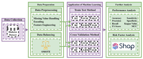
Figure 1.
Experimental methodology of the study for building a diabetes prediction model using socio-demographic characteristics by machine learning techniques.
2.3. Data Balancing Techniques
The synthetic minority oversampling technique (SMOTE) was utilized to balance the imbalanced dataset. SMOTE is an oversampling approach to balance imbalanced data. It is one of the most widely used balancing techniques. It is employed to address imbalance issues. It attempts to balance the number of classes by randomly creating minority class samples and duplicating them. SMOTE introduces unique minority instances by synthesizing existing minority instances [15]. For something like the minority class, linear interpolation is used to create virtual training data. By choosing a random one or several of the k-nearest neighbors for every instance in the minority class, such synthetic training records are constructed. These data are regenerated after the oversampling procedure, and several categorization methods can be used to analyze the data input [16]. It selects instances inside the feature set that are close to each other, draws a line between the instances, and then creates a new instance at a location somewhere along the line.
2.4. Performance Evaluation Metrics
Accuracy and other statistical evaluation metrics were considered to find the best fit ML model among all the applied classifiers. All the applied supervised ML classifiers were compared to each other based on the criteria used to evaluate their efficiency. In most cases, ML models are assessed using sensitivity, specificity, and accuracy; these are generated by a confusion matrix. Classification accuracy is the ratio of the correctly classified models to all other possible outputs. Accuracy is a suitable metric whenever the target feature categories in the data are rather equal [17]. Specificity describes the percentage of true negatives estimated to be negatives [18]. A metric called "Sensitivity" shows the proportion of actual positive events that were assumed to be positive [18]. The following equations are used to determine the value of all the statistical evaluation metrics [17,18].
In addition to these three evaluation metrics, for more precise evaluation, several other evaluation metrics were considered to determine how effectively each algorithm performed. These are Matthew’s correlation coefficient (MCC), kappa statistics, recall, precision, and f1-measure. Matthew’s correlation coefficient (MCC) takes the confusion matrix’s four parameters into account, as well as a maximum level (near to 1) which shows that both classifications are well estimated, even if one category is significantly under- (or over) represented [19,20].Recall is a metric that represents the number of positives that the machine learning (ML) algorithms obtain [21]. This score will calculate the harmonic mean of accuracy and recall. The weighted average of accuracy and recall is utilized to evaluate the F1-score [21]. Precision determines the ratio of true positives to all expected positives [21]. The observed and estimated accuracy is analyzed using the kappa statistic [22]. In the equation, the terms TP, FP, and TN, FN are, respectively, true positive, false positive, true negative, and false negative.
2.5. K-Fold Cross-Validation and Train–Test Split
A five-fold cross-validation (CV) approach is demonstrated in Figure 2. The dataset is broken down into five groups, four of which take part in model training and one of which evaluates model training after each round. A five-fold CV is used in this work. To prevent overfitting inside a classification algorithm, cross-validation is the most efficient method. Train–test split is a traditional approach for ML algorithms. In train–test split, the dataset is broken into two parts; one part is used to train the model, and the rest of the other part is used for testing the model [23]. In this study, we used 70% of the total data for training our ML models, and the remaining 30% of the data we used for testing the model and analyzing the performance of the ML models.
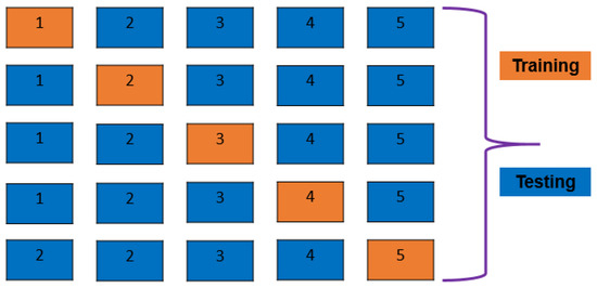
Figure 2.
Visual representation of K-Fold CV method in supervised machine learning model training and testing.
2.6. Machine Learning Algorithms
Several supervised and classified machine learning (ML) approaches were applied in this research. Here are some suggested supervised machine learning (ML) methods for predicting diabetes.
2.6.1. Decision Tree Classifier
Decision tree (DT) is a supervised ML algorithm that can be used in both classification and regression tasks. It consists of a tree-structured classifier, in which each leaf node represents the classification outcome and each inside node represents the attributes of a dataset [24]. A DT consists of two nodes, namely the decision node and the leaf node. Decision nodes are used for taking actions and include some branches; on the other hand, leaf nodes show the results of those decisions and do not consist of any additional branches. Due to the fact that it grows on succeeding branches to form a structure resembling a tree, it is called a "decision tree" because, like a tree, it starts from the root. The leaves stand in for the options or possibilities. These decision nodes split up the data. In terms of decision tree (DT) building, there are two metrics: one is Entropy/Gini-index, and the other is information gain (IG). The two metric calculation equations are shown below.
2.6.2. Random Forest Classifier
Random forest (RF) is a type of ensemble learning and a supervised ML classifier. An ensemble of DTs, the majority of which were trained using the "bagging" method, is combined to create a forest. The bagging approach’s core concept is that, by integrating multiple learning methods, the outcome is improved [25]. Based on voting methods, this supervised learning methodology forecasts the outcome. The random forest (RF) forecasts that the ultimate prediction will be 1, and vice versa, if the majority of the trees in the forest offer a prediction of 1 [26]. Additionally, random forest (RF) is a quantitative approach that applies decision tree classifiers to various resamples of the dataset before using averaging to improve prediction accuracy and prevent overfitting. When bootstrap = True, the max samples option controls the size of the resamples; otherwise, each tree is created using the entire dataset [27]. Random forest (RF) also uses the same metrics that have been used in decision tree (DT) classifiers, such as entropy, entropy/Gini-Index, and information gain (IG). The equation of those metrics is already shown above in the decision tree (DT) subsection.
2.6.3. Support Vector Machine
Support vector machines (SVMs) is a group of supervised learning approaches that address classification tasks, analysis of regression problems, as well as outliers’ identification. Due to their capacity to choose a decision boundary that minimizes the distance from the adjacent data points in all classifications, SVMs differ from other classification algorithms. The decision boundary classifier or the highest margin hyperbolic decision boundary generated by SVMs is referred to as plane and plane. An SVM has two types; the first is simple SVM and the second is kernel SVM [28]. In this study, we used the kernel SVM. On the kernel SVM, we used the linear kernel SVM. The majority of other kernel functions are slower than linear kernel functions, and there are fewer parameters to optimize. The equations that are used by the linear kernel SVM have been described below [28].
Throughout this equation, w stands for the weight matrix to optimize, X for the data to interpret, and b stands for the predicted linear coefficient from either the training dataset or the test dataset. The above equation establishes the output range of the SVM.
2.6.4. XGBoost Classifier
XGBoost (Extreme Gradient Boosting) is a method for ensemble learning. Sometimes, sole reliance on the output of one machine learning (ML) model may not have been effective. A technique for systematically combining the prediction skills of several learners is ensemble learning. As a result, a mono framework that incorporates the output of several models is produced [29]. Additionally, the decentralized gradient boosting framework XGBoost was created to be very effective, flexible, and portable. It develops machine learning (ML) methods using the gradient boosting framework. In order to swiftly and reliably carry out a wide range of data science applications, XGBoost uses concurrent tree boosting [30]. Efficiency and implementation duration were taken into consideration when developing the XGBoost algorithm. In comparison to other boosting algorithms, it works substantially faster. With XGBoost, problems with regression and classification can both be resolved. This method significantly improves the decision tree chain’s weight-dependent efficiency. For this work, we used the default XGBoost algorithm; we did not tune any hyper-parameters of this algorithm.
2.6.5. LightGBM Classifier
The LightGBM/LGBM (light gradient boosting machine) gradient-boosting approach uses concepts from tree-based modeling. It can manage enormous volumes of data due to the decentralized architecture, ability for parallel learning, and use of GPUs. The speed of LGBM is six times that of XGBoost. A rapid and precise machine learning technique is XGBoost. Conversely, LGBM, which executes more rapidly with comparable predictive performance and simply provides additional hyperparameters to modify, potentially poses a threat. The key performance difference is that, whereas LGBM separates the tree vertices one at a time, XGBoost does it one layer at a time [31]. Furthermore, LGBM is a gradient-boosting technique that employs similar tree-based instructional strategies. A different method develops trees parallel to the ground, whereas LGBM produces trees upwardly, or, to put it another way, LGBM produces trees leaf by leaf, whereas another method produces trees level by level. The leaf with the greatest delta erosion will be produced [32]. This study used the default parameter for LGBM classifiers.
2.6.6. Multi-Layer Perceptron
One of the least complex artificial neural network is multi-layer perceptron (MLP). It is a combination of multiple perceptron algorithms. Perceptrons are designed to mimic the functions of a human brain in an attempt to predict future cases.Such perceptrons are orthogonal in MLP and have a significant degree of connectivity. Effective parallel processing facilitates faster computing. Frank Rosenblatt developed the perceptron in 1950. Much like the human brain, it is capable of learning complicated tasks. A perceptron structure (output unit) is made up of a sensory unit (input unit), associator unit (hidden unit), and response unit [33]. A completely associated input layer and an output layer make up the perceptron. The input and output layers of MLPs are the same, but there could be several hidden layers somewhere in the input layer or output layer. The MLP model is developed continuously. The cost function’s partial derivatives are employed to modify each phase’s parameters.
2.7. Feature Importance and Model Explanation
The most significant thing in any ML strategic approach is choosing the appropriate method. While taking into account several assessment matrices and scientifically assessing the results, we chose the superior model for the current study. Showing the feature impact of each model on their prediction is also an essential concept in ML approaches. The features’ impact plays a vital role in building an effective ML model. The features’ impact shows why those features are important in building a specific model and how those features influence the model’s prediction side by side. Showing the features’ impact on the model’s prediction will significantly affect studies for forecasting in the disciplines of social science and healthcare. SHAP (SHapley Additive exPlanations) plots have been utilized in the research to show the features’ impact on the model’s prediction. The significance of receiving a specific value for a specific characteristic in comparison to the forecast we would provide if that attribute had a quantitative amount is quantified by SHAP values [34].
3. Result Analysis and Discussion
In this study, six supervised ML algorithms were employed to build a model to predict diabetes using socio-demographic characteristics in the early stages. Before applying machine learning techniques, exploratory data analysis (EDA) is performed to explore the hidden knowledge of the applied dataset. Then, ML techniques are conducted to build a potential model to predict diabetes and to identify the most significant socio-demographic risk factors related to diabetes. All the findings of this study are represented in this section.
3.1. Exploratory Data Analysis (EDA) Result
Figure 3 depicts the results of exploratory data analysis of the diabetes dataset for all the features. In Figure 3, N refers to the negative, whereas P refers to the positive. In addition to that F, and M refer to females and males, respectively. According to Figure 3, females are more affected by diabetes compared to males. The figure also shows that patients with polyuria, polydipsia, or sudden weight loss are more likely to have diabetes. Of the patients who do not have polyuria, polydipsia, and sudden weight loss, around 70% do not have diabetes. For polyphagia, irritability, partial paresis, and obesity syndromes, patients have a high diabetes risk. Among those who do not have polyphagia, irritability, partial paresis, or obesity, about half have diabetes. According to Figure 3, patients who are more than 30 years old are highly vulnerable to diabetes.
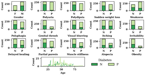
Figure 3.
Exploratory data analysis result.
3.2. Performance Evaluation of ML Models
Six machine learning models such as MLP, SVM, DT, LGBM, XGB, and RF were applied and their performances were compared to each other to find the best-fit model to predict diabetes in the early stage. The results of the ML models are represented in the following sections.
At first, the imbalanced dataset was trained using the train–test split method, where 70% of the dataset was utilized to train the model, and 30% of the dataset was employed for testing the built models. The result of the train–test split method on the imbalanced dataset is represented in Table 2. According to Table 2, the lowest performance is generated by SVM and MLP classifiers. RF has the highest accuracy score of 98.44% among the six ML algorithms. Furthermore, RF also gives the maximum scores for the rest of the performance metrics: precision, recall, f1-score, sensitivity, specificity, kappa statistics, and MCC value, which are, respectively, 0.9800, 0.9899, 0.9849, 0.9785, 0.9899, 0.9687, and 0.9687.
Table 2.
Performance evaluation on imbalance dataset for train–test split method.
Table 3 shows the results for different performance metrics on the imbalanced dataset. RF has the highest accuracy score of 98.44% among the six ML algorithms. Furthermore, RF also gives the maximum scores for the rest of the performance metrics: precision, recall, f1-score, sensitivity, specificity, kappa statistics, and MCC value, which are, respectively, 0.9800, 0.9899, 0.9849, 0.9785, 0.9899, 0.9687, and 0.9687.
Table 3.
Performance evaluation on balance dataset for train test split method.
Table 4 represents detailed information about the ML approaches for five-fold CV results on the balanced dataset. The maximum CV accuracy is 94.87% for RF classifiers. DT shows the highest precision value of 0.9784, and RF gives the highest recall and f1-scores of 0.9608 and 0.9608. At the same time, DT also gains the maximum sensitivity value of 0.9629. The maximum specificity, kappa statistics, and MCC values given through RF are 0.9608, 0.8867, and 0.8867, respectively.
Table 4.
Performance evaluation on balance dataset for five-fold CV method.
The five-fold CV results on the balanced dataset for the ML approaches are described in Table 5. According to Table 5, RF and LGBM have the highest maximum accuracy of 93.23%. Moreover, RF and LGBM show the highest precision value of 0.9574. The highest recall and specificity value is 0.9091, which is generated by DT, RF, XGBoost, and LGBM classifiers. Both RF and LGBM show a maximum sensitivity score of 0.9570. RF and LGBM have shown maximum values of f1-score, kappa statistics, and MCC of 0.9326, 0.8647, and 0.8658, respectively.
Table 5.
Performance evaluation on imbalance dataset for five-fold CV method.
Figure 4 shows the ROC curve and precision–recall (PR) curve for six different ML techniques that have been applied in this study. The results for the balanced dataset are shown in Figure 4A,B. On the other hand, Figure 4C,D show the results of the imbalanced dataset. For a balanced dataset, the highest AUC score is 1.00 for RF, XGBoost, and LGBM, as shown in the figure. At the same time, RF, XGBoost, and LGBM show the highest AUCPR value, which is also 1.00. On the contrary, the maximum AUC score is 0.999, as shown by RF. It is worth noting that RF also shows the highest AUCPR value of 0.999 for an imbalanced dataset.
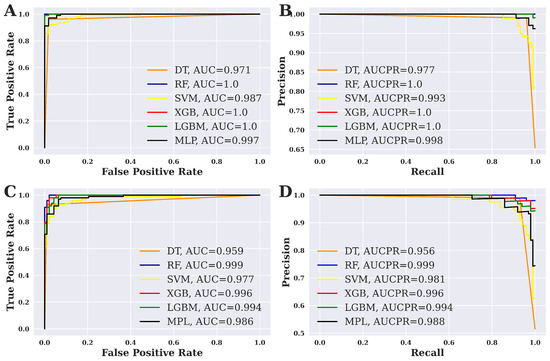
Figure 4.
ROC curve and PR curve analysis. (A) ROC curve for the balanced dataset, (B) PR curve for the balanced dataset, (C) ROC curve for the imbalanced dataset, and (D) PR curve for the imbalanced dataset.
3.3. Overall Performance Evaluation for ML Methods
The results of the performance metrics for six ML approaches are shown in Figure 5. In Figure 5, we compare the results of train–test split and cross-validation techniques for the balanced dataset. It is shown that the results of train–test-split are mostly higher than those of cross-validation. But in a few cases, the results of cross-validation are increasing. For DT, precision and sensitivity show the same results for both train–test split and cross-validation. SVM yields the same recall and specificity results for both techniques. Furthermore, the MLP shows few exceptions; in the MLP, the results of precision and sensitivity for cross-validation are higher than the train–test split’s result.
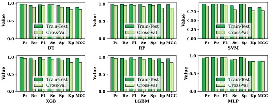
Figure 5.
Comparison of the results of different performance metrics based on train–test split and cross-validation for the balanced dataset.
Figure 6 compares the accuracy of the six ML approaches for both datasets. It has been shown that the balanced dataset’s accuracy is always higher than the imbalanced dataset for all the classifiers that have been used in this research. Among the six ML algorithms, RF shows the highest accuracy for both the dataset and the techniques of train–test split and cross-validation.
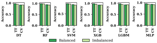
Figure 6.
Accuracy of the six applied classifiers for balanced and imbalanced dataset based on train–test split and cross-validation.
3.4. Risk Factor Analysis and Model Explanation Based on SHAP Value
This study also aims to find the features’ impact on predicting diabetes for different ML techniques. We have utilized the SHAP summary plot to carry out and show the feature’s impact on the models. Using SHAP value, summary plot is depicted to show how the features affect the forecast.It takes into account the absolute SHAP value; hence, it matters if the feature affects the prediction either positively or negatively [35]. The features’ impact on model prediction utilizing the SHAP Summery plot for six ML algorithms is shown in Figure 7.
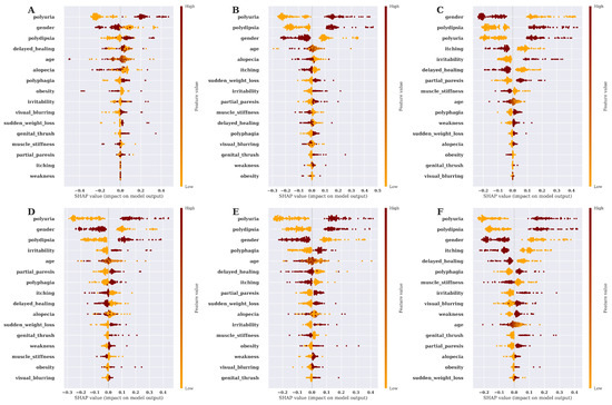
Figure 7.
SHAP summary plot for features’ impact on model prediction. (A) Features’ importance on model prediction by DT, (B) Features’ importance on model prediction by RF, (C) Features’ importance on model prediction by SVM, (D) Features’ importance on model prediction by XGBOOST, (E) Features’ importance on model prediction by LGBM, (F) Features’ importance on model prediction by MLP.
3.5. Discussion
Researchers have conducted a significant amount of research on diabetes prediction, but there is still room for improvement in diabetes prediction research. For predicting diabetes in this work, we employ a socio-demographic diabetes dataset. After collecting the dataset, we pre-processed it to make it suitable for further analysis. We applied six supervised ML algorithms, namely DT, RF, SVM, XGBOOST, LGBM, and MLP to predict diabetes. After applying the ML approaches, we assessed the results of the applied ML approaches utilizing different performance metrics like accuracy, precision, recall, f1-measure, sensitivity, specificity, kappa statistics, and MCC. Among the applied ML algorithms, RF shows the highest result with a 99.37% accuracy; 1.00 precision; 0.9902 recall; 0.9951 f1-score; 1.00 sensitivity; 0.9902 specificity; as well as kappa statistics and MCC of 0.9859 and 0.9860, respectively, for the train–test split technique, which effectively predicts diabetes. The same socio-demographic diabetes dataset that we analyzed for diabetes prediction was also analyzed by Islam, M. M. et al. (2020) and has been shown to have the highest result of 99.00% accuracy for the RF approaches [6]. And Ahmed, Usama et al. (2022) also used the same dataset and obtained a 94.87% accuracy; 0.9552 sensitivity; 0.9438 specificity; and 0.9412 f1-score [11]. The impact of features on the model plays an essential role in the ML field for any disease prediction. Therefore, in this work, we also show the features’ impact on model prediction of the six ML algorithms by utilizing the SHAP summary plot, which is graphically expressed in Figure 7.
According to Table 6, it has been found that our proposed model is highly capable of predicting diabetes using only socio-demographic features. In addition to that, the proposed model is validated by more evaluation metrics than the existing models. The proposed model has some practical application in different fields such as early diabetes risk assessment, customized diabetes prevention plans, community health initiatives, telehealth and remote monitoring, and others. In addition to that, this study will contribute to develop personalized diabetes management apps and personalized medicine. In brief, this study demonstrates many potential real-life applications in the health sector.
Table 6.
Comparison the proposed model with existing methods.
However, this study has some limitations. First of all, the number of instances in this dataset is only 520, which is enough to build an ML-based prediction model but not good enough. As a result, we should collect more data in the future. The attributes of the diabetes dataset are only socio-demographic, but the socio-demographic data on diabetes are not sufficient to accurately predict diabetes. For that reason, we should collect clinical data in the future and merge them together to build an effective diabetes prediction model. Also, in the future, this study should be focused on utilizing more effective ML approaches to build an effective prediction model and develop an end-user website for diabetes prediction. Alongside its weakness, some of the strengths of this study include proposing a low-cost and efficient machine learning model with high accuracy. The model has shown a significant outcome in terms of predicting diabetes in early stages.
4. Conclusions
Diabetes is now one of the most alarming diseases in the world. Data mining and ML are now being used to predict diabetes alongside traditional clinical tests. Inspired by this, this study aimed to build an automated model to predict diabetes at an early stage. To fulfill this objective, six ML approaches were applied and compared to their performances to find the best-fit classifier that will predict diabetes based on a socio-demographic attribute in an early stage with significant accuracy. It was observed that the best-fit classifier is RF with an accuracy of 99.37%. This study also aimed to find the features’ impact on model prediction, and that has been successfully achieved in this study. The proposed method will be further developed with more state-of-the-art technology and with more data in the future. This study presents limitations regarding the data. The findings will be more beneficial for researchers who have an interest in diabetes disease research based on ML techniques and will also be helpful for physicians to diagnose diabetes at very early stages.
Author Contributions
M.A.R., L.F.A., M.M.A., I.M., F.M.B. and K.A. provided the concept and performed the experiments; wrote the paper; analyzed and interpreted the data. M.A.R. and M.M.A. interpreted the data. M.A.R. and M.M.A. handled the manuscript and analyzed the data. K.A. and M.M.A. edited and reviewed the manuscript. F.M.B. provided funding for the project. F.M.B., K.A. and M.M.A. designed the experiments and supervised the whole project. All authors have read and agreed to the published version of the manuscript.
Funding
This research work was funded by the Natural Sciences and Engineering Research Council of Canada (NSERC).
Data Availability Statement
The corresponding author can provide the data that were utilized to support the study upon request.
Conflicts of Interest
No conflict of interest are disclosed by the authors.
References
- Banerjee, A.T.; Shah, B.R. Differences in prevalence of diabetes among immigrants to Canada from South Asian countries. Diabet. Med. 2018, 35, 937–943. [Google Scholar] [CrossRef] [PubMed]
- Roglic, G. WHO Global report on diabetes: A summary. Int. J. Noncommun. Dis. 2016, 1, 3. [Google Scholar] [CrossRef]
- Zou, Q.; Qu, K.; Luo, Y.; Yin, D.; Ju, Y.; Tang, H. Predicting diabetes mellitus with machine learning techniques. Front. Genet. 2018, 9, 515. [Google Scholar] [CrossRef] [PubMed]
- Balfe, M.; Doyle, F.; Smith, D.; Sreenan, S.; Brugha, R.; Hevey, D.; Conroy, R. What’s distressing about having type 1 diabetes? A qualitative study of young adults’ perspectives. BMC Endocr. Disord. 2013, 13, 25. [Google Scholar] [CrossRef] [PubMed]
- Khanam; Jamal, J.; Foo, S.Y. A comparison of machine learning algorithms for diabetes prediction. ICT Express 2021, 7, 432–439. [Google Scholar] [CrossRef]
- Islam, M.M.F.; Ferdousi, R.; Rahman, S.; Bushra, H.Y. Likelihood prediction of diabetes at early stage using data mining techniques. In Computer Vision and Machine Intelligence in Medical Image Analysis; Springer: Singapore, 2020; pp. 113–125. [Google Scholar]
- Krishnamoorthi, R.; Joshi, S.; Almarzouki, H.Z.; Shukla, P.K.; Rizwan, A.; Kalpana, C.; Tiwari, B. A novel diabetes healthcare disease prediction framework using machine learning techniques. J. Healthc. Eng. 2022, 2022, 1684017. [Google Scholar] [CrossRef]
- Islam, M.S.; Qaraqe, M.K.; Belhaouari, S.B.; Abdul-Ghani, M.A. Advanced techniques for predicting the future progression of type 2 diabetes. IEEE Access 2020, 8, 120537–120547. [Google Scholar] [CrossRef]
- Hasan, M.K.; Alam, M.A.; Das, D.; Hossain, E.; Hasan, M. Diabetes prediction using ensembling of dif-ferent machine learning classifiers. IEEE Access 2020, 8, 76516–76531. [Google Scholar] [CrossRef]
- Fazakis, N.; Kocsis, O.; Dritsas, E.; Alexiou, S.; Fakotakis, N.; Moustakas, K. Machine learning tools for long-term type 2 diabetes risk prediction. IEEE Access 2021, 9, 103737–103757. [Google Scholar] [CrossRef]
- Ahmed, U.; Issa, G.F.; Khan, M.A.; Aftab, S.; Khan, M.F.; Said, R.A.T.; Ghazal, T.M.; Ahmad, M. Predic-tion of diabetes empowered with fused machine learning. IEEE Access 2022, 10, 8529–8538. [Google Scholar] [CrossRef]
- Maniruzzaman, M.; Rahman, M.J.; Ahammed, B.; Abedin, M.M. Classification and prediction of diabetes disease using machine learning paradigm. Health Inf. Sci. Syst. 2020, 8, 7. [Google Scholar] [CrossRef] [PubMed]
- Barakat, N.; Bradley, A.P.; Barakat, M.N.H. Intelligible support vector machines for diagnosis of diabetes mellitus. IEEE Trans. Inf. Technol. Biomed. 2010, 14, 1114–1120. [Google Scholar] [CrossRef] [PubMed]
- Dataset. Available online: https://www.kaggle.com/datasets/andrewmvd/early-diabetes-classification (accessed on 17 November 2022).
- Chawla, N.V.; Bowyer, K.W.; Hall, L.O.; Kegelmeyer, W.P. SMOTE: Synthetic minority over-sampling technique. J. Artif. Intell. Res. 2002, 16, 321–357. [Google Scholar] [CrossRef]
- Maulidevi, N.U.; Surendro, K. SMOTE-LOF for noise identification in imbalanced data classification. J. King Saud Univ.-Comput. Inf. Sci. 2022, 34, 3413–3423. [Google Scholar]
- Sanni, R.R.; Guruprasad, H.S. Analysis of performance metrics of heart failured patients using Python and machine learning algorithms. Glob. Transit. Proc. 2021, 2, 233–237. [Google Scholar] [CrossRef]
- Silva, F.R.; Vidotti, V.G.; Cremasco, F.; Dias, M.; Gomi, E.S.; Costa, V.P. Sensitivity and specificity of machine learning classifiers for glaucoma diagnosis using Spectral Domain OCT and standard automated perimetry. Arq. Bras. De Oftalmol. 2013, 76, 170–174. [Google Scholar] [CrossRef] [PubMed]
- Chicco, D.; Tötsch, N.; Jurman, G. The Matthews correlation coefficient (MCC) is more reliable than balanced accuracy, bookmaker informedness, and markedness in two-class confusion matrix evaluation. Bio-Data Min. 2021, 14, 13. [Google Scholar] [CrossRef]
- Chicco, D.; Jurman, G. The advantages of the Matthews correlation coefficient (MCC) over F1 score and accuracy in binary classification evaluation. BMC Genom. 2020, 21, 6. [Google Scholar] [CrossRef]
- Erickson, B.J.; Kitamura, F. Magician’s corner: 9. Performance metrics for machine learning models. Radiol. Artif. Intell. 2021, 3, E200126. [Google Scholar] [CrossRef]
- Mohamed, A.E. Comparative study of four supervised machine learning techniques for classification. Int. J. Appl. 2017, 7, 5–18. [Google Scholar]
- Tan, J.; Yang, J.; Wu, S.; Chen, G.; Zhao, J. A critical look at the current train/test split in machine learning. arXiv 2021, arXiv:2106.04525. [Google Scholar]
- Sheth, V.; Tripathi, U.; Sharm, A. Comparative analysis of decision tree classification algorithms. Int. J. Curr. Eng. Technol. 2013, 3, 334–337. [Google Scholar]
- Azar, A.T.; Elshazly, H.I.; Hassanien, A.E.; Elkorany, A.M. A random forest classifier for lymph diseases. Comput. Methods Programs Biomed. 2014, 113, 465–473. [Google Scholar] [CrossRef] [PubMed]
- Song, Y.Y.; Ying, L.U. Decision tree methods: Applications for classification and prediction. Shanghai Arch. Psychiatry 2015, 27, 130. [Google Scholar] [PubMed]
- Liaw, A.; Wiener, M. Classification and regression by randomForest. R News 2002, 2, 18–22. [Google Scholar]
- Zhang, Y. Support vector machine classification algorithm and its application. In Proceedings of the Information Computing and Applications: Third International Conference, ICICA 2012, Chengde, China, 14–16 September 2012; Proceedings, Part II 3. Springer: Berlin/Heidelberg, Germany, 2012. [Google Scholar]
- Santhanam, R.; Uzir, N.; Raman, S.; Banerjee, S. Experimenting XGBoost algorithm for prediction and classification of different datasets. Int. J. Control Theory Appl. 2016, 9, 651–662. [Google Scholar]
- XGBoost Documentation. Available online: https://xgboost.readthedocs.io/en/stable/ (accessed on 24 December 2022).
- Rufo, D.D.; Debelee, T.G.; Ibenthal, A.; Negera, W.G. Diagnosis of diabetes mellitus using gradient boosting machine (LightGBM). Diagnostics 2021, 11, 1714. [Google Scholar] [CrossRef] [PubMed]
- Abdurrahman, M.H.; Irawan, B.; Setianingsih, C. A review of light gradient boosting machine method for hate speech classification on twitter. In Proceedings of the 2020 2nd International Conference on Electrical, Control and Instrumentation Engineering (ICECIE), Kuala Lumpur, Malaysia, 28 November 2020. [Google Scholar]
- Desai, M.; Shah, M. An anatomization on breast cancer detection and diagnosis employing multi-layer perceptron neural network (MLP) and Convolutional neural network (CNN). Clin. Ehealth 2021, 4, 1–11. [Google Scholar] [CrossRef]
- Marcílio, W.E.; Eler, D.M. From explanations to feature selection: Assessing SHAP values as feature selection mechanism. In Proceedings of the 2020 33rd SIBGRAPI Conference on Graphics, Patterns and Images (SIBGRAPI), Porto de Galinhas, Brazil, 7–10 November 2020. [Google Scholar]
- Bowen, D.; Ungar, L. Generalized SHAP: Generating multiple types of explanations in machine learning. arXiv 2020, arXiv:2006.07155. [Google Scholar]
Disclaimer/Publisher’s Note: The statements, opinions and data contained in all publications are solely those of the individual author(s) and contributor(s) and not of MDPI and/or the editor(s). MDPI and/or the editor(s) disclaim responsibility for any injury to people or property resulting from any ideas, methods, instructions or products referred to in the content. |
© 2023 by the authors. Licensee MDPI, Basel, Switzerland. This article is an open access article distributed under the terms and conditions of the Creative Commons Attribution (CC BY) license (https://creativecommons.org/licenses/by/4.0/).