Deep Neural Networks Training by Stochastic Quasi-Newton Trust-Region Methods

Abstract

While first-order methods are popular for solving optimization problems arising in deep learning, they come with some acute deficiencies. To overcome these shortcomings, there has been recent interest in introducing second-order information through quasi-Newton methods that are able to construct Hessian approximations using only gradient information. In this work, we study the performance of stochastic quasi-Newton algorithms for training deep neural networks. We consider two well-known quasi-Newton updates, the limited-memory Broyden–Fletcher–Goldfarb–Shanno (BFGS) and the symmetric rank one (SR1). This study fills a gap concerning the real performance of both updates in the minibatch setting and analyzes whether more efficient training can be obtained when using the more robust BFGS update or the cheaper SR1 formula, which—allowing for indefinite Hessian approximations—can potentially help to better navigate the pathological saddle points present in the non-convex loss functions found in deep learning. We present and discuss the results of an extensive experimental study that includes many aspects affecting performance, like batch normalization, the network architecture, the limited memory parameter or the batch size. Our results show that stochastic quasi-Newton algorithms are efficient and, in some instances, able to outperform the well-known first-order Adam optimizer, run with the optimal combination of its numerous hyperparameters, and the stochastic second-order trust-region STORM algorithm.

1. Introduction

Deep learning (DL), as a leading technique of machine learning (ML), has attracted much attention and has become one of the most popular directions of research. DL approaches have been applied to solve many large-scale problems in different fields, e.g., automatic machine translation, image recognition, natural language processing, fraud detection, etc., by training deep neural networks (DNNs) over large available datasets. DL problems are often posed as unconstrained optimization problems. In supervised learning, the goal is to minimize the empirical risk:

$$\underset{w\in {\mathbb{R}}^n}{min}F\left(w\right)\triangleq \frac{1}{N}\sum _{i=1}^{N}L(y_i,h(x_i;w))\triangleq \frac{1}{N}\sum _{i=1}^N{L}_i\left(w\right),$$

(1)

by finding an optimal parametric mapping function $h(·;w):{\mathbb{R}}^d⟶{\mathbb{R}}^C$, where $w\in {\mathbb{R}}^n$ is the vector of the trainable parameters of a DNN and $(x_i,y_i)$ denotes the ith sample pair in the available training dataset ${\left\{(x_i,y_i)\right\}}_{i=1}^N$ with converted input $x_i\in {\mathbb{R}}^d$ and a one-hot true target $y_i\in {\mathbb{R}}^C$. Moreover, $L_i(.,.)\in \mathbb{R}$ is a loss function defining the prediction error between $y_i$ and the DNN’s output $h(x_i;.)$. Problem (1) is highly nonlinear and often non-convex and, thus, applying traditional optimization algorithms is ineffective.

Optimization methods for problem (1) can be divided into first-order and second-order methods, where the gradient and Hessian (or a Hessian approximation) are used, respectively. These methods, in turn, fall into two broad categories, stochastic and deterministic, in which either one sample (or a small subset of samples called minibatch) or a single batch composed of all samples are, respectively, employed in the evaluation of the objective function or its gradient.

In DL applications, both N and n can be very large; thus, computing the full gradient is expensive, and computations involving the true Hessian or its approximation may not be practical. Recently, much effort has been devoted to the development of DL optimization algorithms. Stochastic optimization methods have become the usual approach to overcoming the aforementioned issues.

1.1. Review of the Literature

Stochastic first-order methods have been widely used in many DL applications, due to their low per-iteration cost, optimal complexity, easy implementation, and proven efficiency in practice. The preferred method is the stochastic gradient descent (SGD) method [1,2], and its variance-reduced [3,4,5] and adaptive [6,7] variants. However, due to the use of first-order information only, these methods come with several issues, such as relatively slow convergence, high sensitivity to the choice of hyperparameters (e.g., step length and batch size), stagnation at high training loss, difficulty in escaping saddle points [8], the limited benefits of parallelism, due to the usual implementation with small minibatches, and suffering from ill-conditioning [9].

On the other hand, second-order methods can often find good minima in fewer steps, due to their use of curvature information. The main second-order method incorporating the inverse Hessian matrix is Newton’s method [10], but it presents serious computational and memory usage challenges involved in the computation of the Hessian, in particular for large-scale DL problems; see [11] for details.

Quasi-Newton [10] and Hessian-free Newton methods [12] are two techniques aimed at incorporating second-order information without computing and storing the true Hessian matrix. Hessian-free methods attempt to find an approximate Newton direction, using conjugate gradient methods [13,14,15]. The major challenge of these methods is the linear system with an indefinite subsampled Hessian matrix and (subsampled) gradient vector to be solved at each Newton step. This problem can be solved in the trust region framework by the CG–Steihaug algorithm [16]. Nevertheless, whether true Hessian matrix–vector products or subsampled variants of them (see, e.g., [15]) are used, the iteration complexity of a (modified) CG algorithm is significantly greater than that of a limited-memory quasi-Newton method, i.e., stochastic L-BFGS; see the complexity table in [15]. Quasi-Newton methods and their limited memory variants [10] attempt to combine the speed of Newton’s method and the scalability of first-order methods. They construct Hessian approximations, using only gradient information, and they exhibit superlinear convergence. All these methods can be implemented to benefit from parallelization in the evaluations of the objective function and its derivatives, which is possible, due to their finite sum structure [11,17,18].

Quasi-Newton and stochastic quasi-Newton methods to solve large optimization problems arising in machine learning have been recently extensively considered within the context of convex and non-convex optimization. Stochastic quasi-Newton methods use a subsampled Hessian approximation or/and a subsampled gradient. In [19], a stochastic Broyden–Fletcher–Goldfarb–Shanno (BFGS) and its limited memory variant (L-BFGS) were proposed for online convex optimization in [19]. Another stochastic L-BFGS method for solving strongly convex problems was presented in [20] that uses sampled Hessian-vector products rather than gradient differences, which was proved in [21] to be linearly convergent by incorporating the SVRG variance reduction technique [4] to alleviate the effect of noisy gradients. A closely related variance-reduced block L-BFGS method was proposed in [22]. A regularized stochastic BFGS method was proposed in [23], and an online L-BFGS method was proposed in  [24] for strongly convex problems and extended in [25] to incorporate SVRG variance reduction. For the solution of non-convex optimization problems arising in deep learning, a damped L-BFGS method incorporating SVRG variance reduction was developed and its convergence properties were studied in [26]. Some of these stochastic quasi-Newton algorithms employ fixed-size batches and compute stochastic gradient differences in a stable way, originally proposed in [19], using the same batch at the beginning and at the end of the iteration. As this can potentially double the iteration complexity, an overlap batching strategy was proposed, to reduce the computational cost in [27], and it was also tested, in [28]. This strategy was further applied in [29,30]. Other stochastic quasi-Newton methods have been considered that employ a progressive batching approach in which the sample size is increased as the iteration progresses; see, e.g., [31,32] and references therein. Recently, in [33], a Kronecker-factored block diagonal BFGS and L-BFGS method was proposed, which takes advantage of the structure of feed-forward DNN training problems.

1.2. Contribution and Outline

The BFGS update is the most widely used type of quasi-Newton method for general optimization and the most widely considered quasi-Newton method for general machine learning and deep learning. Almost all the previously cited articles considered BFGS, with only a few exceptions using the symmetric rank one (SR1) update instead [29]. However, a clear disadvantage of BFGS occurs if one tries to enforce the positive-definiteness of the approximated Hessian matrices in a non-convex setting. In this case, BFGS has the difficult task of approximating an indefinite matrix (the true Hessian) with a positive-definite matrix which can result in the generation of nearly singular Hessian approximations.

In this paper, we analyze the behavior of both updates on real modern deep neural network architectures and try to determine whether more efficient training can be obtained when using the BFGS update or the cheaper SR1 formula that allows for indefinite Hessian approximations and, thus, can potentially help to better navigate the pathological saddle points present in the non-convex loss functions found in deep learning. We would like to determine whether better training results could be achieved by using SR1 updates, as these allow for indefinite Hessian approximations. We study the performance of both quasi-Newton methods in the trust region framework for solving (1) in realistic large-size DNNs. We introduce stochastic variants of the two quasi-Newton updates, based on an overlapping sampling strategy which is well-suited to trust-region methods. We have implemented and applied these algorithms to train different convolutional and residual neural networks, ranging from a shallow LeNet-like network to a self-built network with and without batch normalization layers and the modern ResNet-20, for image classification problems. We have compared the performance of both stochastic quasi-Newton trust-region methods with another stochastic quasi-Newton algorithm based on a progressive batching strategy and with the first-order Adam optimizer running with the optimal values of its hyperparameters, obtained by grid searching.

The rest of the paper is organized as follows: Section 2 provides a general overview of trust-region quasi-Newton methods for solving problem (1) and introduces the stochastic algorithms sL-BFGS-TR and sL-SR1-TR, together with a suitable minibatch sampling strategy. The results of an extensive empirical study on the performance of the considered algorithms in the training of deep neural networks are presented and discussed in Section 3. Finally, some concluding remarks are given in Section 4.

2. Materials and Methods

We provide in this section an overview of quasi-Newton trust-region methods in the deterministic setting and introduce suitable stochastic variants.

Trust-region (TR) methods [34] are powerful techniques for solving nonlinear unconstrained optimization problems that can incorporate second-order information, without requiring it to be positive-definite. TR methods generate a sequence of iterates, $w_k+p_k$, such that the search direction $p_k$ is obtained by solving the following TR subproblem,

$$p_k=arg\underset{p\in {\mathbb{R}}^n}{min}{Q}_k\left(p\right)\triangleq \frac{1}{2}{p}^T{B}_{k}p+g_k^{T}p\mathrm{s}.\mathrm{t}.{∥p∥}_2\le {\delta }_k,$$

(2)

for some TR radius ${\delta }_k>0$, where

$$g_k\triangleq \nabla F\left(w_k\right)=\frac{1}{N}\sum _{i=1}^N\nabla L_i\left(w_k\right)$$

(3)

and $B_k$ is a Hessian approximation. For quasi-Newton trust-region methods, the symmetric quasi-Newton (QN) matrices $B_k$ in (2) are approximations to the Hessian matrix constructed using gradient information, and they satisfy the following secant equation:

$$B_{k+1}{s}_k=y_k,$$

(4)

where

$$s_k=p_k,y_k=g_t-g_k,$$

(5)

in which $g_t$ is the gradient evaluated at $w_t=w_k+p_k$. The trial point is subject to the value of the ratio of actual to predicted reduction in the objective function of (1), that is:

$${\rho }_k=\frac{f_k-f_t}{Q_k(0)-Q_k\left(p_k\right)},$$

(6)

where $f_t$ and $f_k$ are the objective function values at $w_t$ and $w_k$, respectively. Therefore, since the denominator in (6) is non-negative, if ${\rho }_k$ is positive then $w_{k+1}\triangleq w_t$; otherwise, $w_{k+1}\triangleq w_k$. Based on the value of (6), the step may be accepted or rejected. Moreover, it is safe to expand ${\delta }_k\in ({\delta }_0,{\delta }_{max})$ with ${\delta }_0,{\delta }_{max}>0$ when there is very good agreement between the model and function. However, the current ${\delta }_k$ is not altered if there is good agreement, or it is shrunk when there is weak agreement. Algorithm 1 describes the TR radius adjustment.

Algorithm 1 Trust region radius adjustment

1: Inputs: Current iteration k, ${\delta }_k$, ${\rho }_k$, $0<{\tau }_2<0.5<{\tau }_3<1$, $0<{\eta }_2\le 0.5$, $0.5<{\eta }_3<1<{\eta }_4$ 2: if ${\rho }_k>{\tau }_3$ then 3:    if $\parallel p_k\parallel \le {\eta }_3{\delta }_k$ then 4:      ${\delta }_{k+1}={\delta }_k$ 5:    else 6:      ${\delta }_{k+1}={\eta }_4{\delta }_k$ 7:    end if 8: else if ${\tau }_2\le {\rho }_k\le {\tau }_3$ then 9:    ${\delta }_{k+1}={\delta }_k$ 10: else 11:    ${\delta }_{k+1}={\eta }_2{\delta }_k$ 12: end if

A primary advantage of using TR methods is their ability to work with both positive-definite and indefinite Hessian approximations. Moreover, the progress of the learning process will not stop or slow down even in the presence of occasional step rejection, i.e., when $w_{k+1}\triangleq w_k$.

Using the Euclidean norm (2-norm) to define the subproblem (2) leads to characterizing the global solution of (2) by the optimality conditions given in the following theorem from Gay [35] and Moré and Sorensen [36]:

Theorem 1.

Let ${\delta }_k$ be a given positive constant. A vector $p_k\triangleq p^{*}$ is a global solution of the trust region problem (2) if and only if ${∥p^{*}∥}_2\le {\delta }_k$ and there exists a unique ${\sigma }^{*}\ge 0$, such that $B_k+{\sigma }^{*}I$ is positive semi-definite with

$$(B_k+{\sigma }^{*}I)p^{*}=-g_k,{\sigma }^{*}({\delta }_k-{∥p^{*}∥}_2)=0.$$

(7)

Moreover, if $B_k+{\sigma }^{*}I$ is positive-definite, then the global minimizer is unique.

According to [37,38], the subproblem (2) or, equivalently, the optimality conditions (7) can be efficiently solved if the Hessian approximation $B_k$ is chosen to be a QN matrix. In the following sections, we provide a comprehensive description of two methods in a TR framework with limited memory variants of two well-known QN Hessian approximations, i.e., L-BFGS and L-SR1.

2.1. The L-BFGS-TR Method

BFGS is the most popular QN update in the Broyden class; that is, it provides a Hessian approximation $B_k$, for which (4) holds. It has the following general form:

$$B_{k+1}=B_k-{\displaystyle \frac{B_k{s}_k{s}_k^T{B}_k}{s_k^T{B}_k{s}_k}}+{\displaystyle \frac{y_k{y}_k^T}{y_k^T{s}_k}},k=0,1,\dots ,$$

(8)

which is a positive-definite matrix, i.e., $B_{k+1}\succ 0$ if $B_0\succ 0$ and the curvature condition holds, i.e., $s_k^T{y}_k>0$. The difference between the symmetric approximations $B_k$ and $B_{k+1}$ is a rank-two matrix. In this work, we bypass updating $B_k$ if the following curvature condition is not satisfied for $\tau ={10}^{-2}$:

$$s_k^T{y}_k>\tau {\parallel s_k\parallel }^2.$$

(9)

For large-scale optimization problems, using the limited-memory BFGS (L-BFGS) would be more efficient. In practice, only a collection of the most recent pairs $\left\{s_j,y_j\right\}$ is stored in memory: for example, l pairs, where $l\ll n$ (usually $l<100$). In fact, for $k\ge l$, the l recent computed pairs are stored in the following matrices $S_k$ and $Y_k$:

$$S_k\triangleq \left[\begin{array}{cccc}{s}_{k-l}& s_{k-(l-1)}& \cdots & s_{k-1}\end{array}\right],Y_k\triangleq \left[\begin{array}{cccc}{y}_{k-l}& y_{k-(l-1)}& \cdots & y_{k-1}\end{array}\right].$$

(10)

Using (10), the L-BFGS matrix $B_k$ can be represented in the following compact form:

$$B_k=B_0+{\Psi }_k{M}_k{\Psi }_k^T,k=1,2,\dots ,$$

(11)

where $B_0\succ 0$ and

$${\Psi }_k=\left[\begin{array}{cc}{B}_0{S}_k& Y_k\end{array}\right],M_k={\left[\begin{array}{cc}-S_k^T{B}_0{S}_k& -L_k\\ -L_k^T& D_k\end{array}\right]}^{-1}.$$

(12)

We note that ${\Psi }_k$ and $M_k$ have at most $2l$ columns. In (12), matrices $L_k$, $U_k$, and $D_k$ are, respectively, the strictly lower triangular part, the strictly upper triangular part, and the diagonal part of the following matrix splitting:

$$S_k^T{Y}_k=L_k+D_k+U_k.$$

(13)

Let $B_0={\gamma }_{k}I$. A heuristic and conventional method of choosing ${\gamma }_k$ is

$${\gamma }_k=\frac{y_{k-1}^T{y}_{k-1}}{y_{k-1}^T{s}_{k-1}}\triangleq {\gamma }_k^h.$$

(14)

The quotient of (14) is an approximation to an eigenvalue of ${\nabla }^{2}F\left(w_k\right)$ and appears to be the most successful choice in practice [10]. Evidently, the selection of ${\gamma }_k$ is important in generating Hessian approximations $B_k$. In DL optimization, the positive-definite L-BFGS matrix $B_k$ has the difficult task of approximating the possibly indefinite true Hessian. According to [29,30], an extra condition can be imposed on ${\gamma }_k$, to avoid false negative curvature information, i.e., to avoid $p_k^T{B}_k{p}_k<0$ whenever $p_k^T{\nabla }^2\left(w_k\right)p_k>0$. Let, for simplicity, the objective function of (1) be a quadratic function:

$$F\left(w\right)=\frac{1}{2}{w}^{T}Hw+g^{T}w,$$

(15)

where $H={\nabla }^{2}F\left(w\right)$, which results in $\nabla F\left(w_{k+1}\right)-\nabla F\left(w_k\right)=H(w_{k+1}-w_k)$ and, thus, $y_k=H{s}_k$ for all k. Thus, we obtain $S_k^T{Y}_k=S_k^{T}H{S}_k$. For the quadratic model, and using (11), we obtain

$$S_k^{T}H{S}_k-{\gamma }_k{S}_k^T{S}_k=S_k^T{\Psi }_k{M}_k{\Psi }_k^T{S}_k.$$

(16)

According to (16), if H is not positive-definite, then its negative curvature information can be captured by $S_k^T{\Psi }_k{M}_k{\Psi }_k^T{S}_k$ as ${\gamma }_k>0$. However, false curvature information can be produced when the ${\gamma }_k$ value chosen is too large while H is positive-definite. To avoid this, ${\gamma }_k$ is selected in $(0,\hat{\lambda })$, where $\hat{\lambda }$ is the smallest eigenvalue of the following generalized eigenvalue problem:

$$(L_k+D_k+L_k^T)u=\lambda S_k^T{S}_{k}u,$$

(17)

with $L_k$ and $D_k$ defined in (13). Therefore, if $\hat{\lambda }\le 0$, then ${\gamma }_k$ is the maximum value of 1 and ${\gamma }_k^h$ defined in (14). Given ${\gamma }_k$, the compact form (11) is applied in (7), where both optimality conditions together are solved for $p_k\triangleq p_k^{*}$ through Algorithm A1 included in Appendix B. Then, according to the value of (6), the step $w_k+p_k$ may be accepted or rejected.

2.2. The L-SR1-TR Method

Another popular QN update in the Broyden class is the SR1 formula, which generates good approximations to the true Hessian matrix, often better than the BFGS approximations [10]. The SR1 updating formula verifying the secant condition (4) is given by

$$B_{k+1}=B_k+{\displaystyle \frac{(y_k-B_k{s}_k){(y_k-B_k{s}_k)}^T}{{(y_k-B_k{s}_k)}^T{s}_k}},k=0,1,\dots .$$

(18)

In this case, the difference between the symmetric approximations $B_k$ and $B_{k+1}$ is a rank-one matrix. To prevent the vanishing of the denominator in (18), a simple safeguard that performs well in practice is to simply skip the update if the denominator is small [10], i.e., $B_{k+1}=B_k$. Therefore, the update (18) is applied only if

$$|s^T(y_k-B_k{s}_k)|\ge \tau \parallel s_k\parallel \parallel y_k-B_k{s}_k\parallel ,$$

(19)

where $\tau \in (0,1)$ is small, say $\tau ={10}^{-8}$. In (18), if $B_k$ is positive-definite, $B_{k+1}$ may not have the same property. Regardless of the sign of $y_k^T{s}_k$ for each k, the SR1 method generates a sequence of matrices that may be indefinite. We note that the value of the quadratic model in (2) evaluated at the descent direction $p^{*}$ is always less if this direction is also a direction of negative curvature. Therefore, the ability to generate indefinite approximations can actually be regarded as one of the chief advantages of SR1 updates in non-convex settings, like in DL applications.

In the limited-memory version of the SR1 (L-SR1) update, as in L-BFGS, only the l most recent curvature pairs are stored in matrices $S_k$ and $Y_k$ defined in (10). Using $S_k$ and $Y_k$, the L-SR1 matrix $B_k$ can be represented in the following compact form:

$$B_k=B_0+{\Psi }_k{M}_k{\Psi }_k^T,k=1,2,,\dots ,$$

(20)

where $B_0={\gamma }_{k}I$ for some ${\gamma }_k\ne 0$ and

$${\Psi }_k=Y_k-B_0{S}_k,M_k={(D_k+L_k+L_k^T-S_k^T{B}_0{S}_k)}^{-1}.$$

(21)

In (21), $L_k$ and $D_k$ are, respectively, the strictly lower triangular part and the diagonal part of $S_k^T{Y}_k$. We note that ${\Psi }_k$ and $M_k$ in the L-SR1 update have, at most, l columns.

In [29], it was proven that the trust region subproblem solution becomes closely parallel to the eigenvector corresponding to the most negative eigenvalue of the L-SR1 approximation $B_k$. This shows the importance of $B_k$ to be able to capture curvature information correctly. On the other hand, it was highlighted how the choice of $B_0={\gamma }_{k}I$ affects $B_k$; in fact, not choosing ${\gamma }_k$ judiciously in relation to $\hat{\lambda }$, the smallest eigenvalue of (17), can have adverse effects. Selecting ${\gamma }_k>\hat{\lambda }$ can result in false curvature information. Moreover, if ${\gamma }_k$ is too close to $\hat{\lambda }$ from below, then $B_k$ becomes ill-conditioned. If ${\gamma }_k$ is too close to $\hat{\lambda }$ from above, then the smallest eigenvalue of $B_k$ becomes negatively large arbitrarily. According to [29], the following lemma suggests selecting ${\gamma }_k$ near but strictly less than $\hat{\lambda }$, to avoid asymptotically poor conditioning while improving the negative curvature approximation properties of $B_k$.

Lemma 1.

For a given quadratic objective function (15), let $\hat{\lambda }$ denote the smallest eigenvalue of the generalized eigenvalue problem (17). Then, for all ${\gamma }_k<\hat{\lambda }$, the smallest eigenvalue of $B_k$ is bounded above by the smallest eigenvalue of H in the span of $S_k$, i.e., 

$${\lambda }_{min}\left(B_k\right)\le \underset{S_{k}v\ne 0}{min}{\displaystyle \frac{v^T{S}_k^{T}H{S}_{k}v}{v^T{S}_k^T{S}_{k}v}}.$$

In this work, we set ${\gamma }_k=max\{{10}^{-6},0.5\hat{\lambda }\}$ in the case where $\hat{\lambda }>0$; otherwise, the ${\gamma }_k$ is set to ${\gamma }_k=min\{-{10}^{-6},1.5\hat{\lambda }\}$. Given ${\gamma }_k$, the compact form (20) is applied in (7), where the optimality conditions together are solved for $p_k$ through Algorithm A2 included in Appendix B, using the spectral decomposition of $B_k$ as well as the Sherman–Morrison–Woodbury formula [38]. Then, according to the value of (6), the step $w_k+p_k$ may be accepted or rejected.

2.3. Stochastic Variants of L-BFGS-TR and L-SR1-TR

The main motivation behind the use of stochastic optimization algorithms in deep learning may be traced back to the existence of a special type of redundancy due to similarity between the data points in (1). In addition, the computation of the true gradient is expensive and the computation of the true Hessian is not practical in large-scale DL problems. Indeed, depending on the available computing resources, it could take a prohibitive amount of time to process the whole set of data examples as a single batch at each iteration of a deterministic algorithm. That is why most of the optimizers in DL work in the stochastic regime. In this regime, the training set ${\left\{(x_i,y_i)\right\}}_{i=1}^N$ is divided randomly into multiple—e.g., $\overline{N}$—batches. Then, a stochastic algorithm uses a single batch $J_k$ at iteration k to compute the required quantities, i.e., stochastic loss and stochastic gradient, as follows:

$$f_k^{J_k}\triangleq F^{J_k}\left(w_k\right)=\frac{1}{|J_k|}\sum _{i\in J_k^{idx}}{L}_i\left(w_k\right),g_k^{J_k}\triangleq \nabla F^{J_k}\left(w_k\right)=\frac{1}{|J_k|}\sum _{i\in J_k^{idx}}\nabla L_i\left(w_k\right),$$

(22)

where $bs\triangleq |J_k|$ and $J_k^{idx}$ denote the size of $J_k$ and the index set of the samples belonging to $J_k$, respectively. In other words, the stochastic QN extensions (sQN) are obtained by replacement of the full loss $f_k$ and gradient $g_k$ in (3) by $f_k^{J_k}$ and $g_k^{J_k}$, respectively, throughout the iterative process of the algorithms. The process of randomly taking $J_k$, computing the required quantities (22) for finding a search direction, and then updating $w_k$ constitutes one single iteration of a stochastic algorithm. This process is repeated for a given number of batches until one epoch (i.e., one pass through the whole set of data samples) is completed. At that point, the dataset is shuffled and new batches are generated for the next epoch; see Algorithms 2 and 3 for a description of the stochastic algorithms sL-BFGS-TR and sL-SR1-TR, respectively.

Algorithm 2 sL-BFGS-TR

1: Inputs: $w_0\in {\mathbb{R}}^n$, $os$, ${\mathrm{epoch}}_{max}$, l, ${\gamma }_0>0$, c, $S_0=Y_0=[.]$, $0<\tau ,{\tau }_1<1$ 2: for $k=0,1,\dots$ do 3:    Take a random and uniform multi-batch $J_k$ of size $bs$ and compute $f_k^{J_k}$, $g_k^{J_k}$ by (22) 4:    if $\mathrm{epoch}>{\mathrm{epoch}}_{max}$ then 5:      Stop training 6:    end if 7:    Compute $p_k$ using Algorithm A1 8:    Compute $w_t=w_k+p_k$ and $f_t^{J_k}$, $g_t^{J_k}$ by (22) 9:    Compute $(s_k,y_k)=(w_t-w_k,g_t^{J_k}-g_k^{J_k})$ and ${\rho }_k={\displaystyle \frac{f_t^{J_k}-f_k^{J_k}}{Q\left(p_k\right)}}$ 10:    if ${\rho }_k\ge {\tau }_1$ then 11:      $w_{k+1}=w_t$ 12:    else 13:      $w_{k+1}=w_k$ 14:    end if 15:    Update ${\delta }_k$ by Algorithm 1 16:    if $s_k^T{y}_k>\tau {\parallel s_k\parallel }^2$ then 17:      Update storage matrices $S_{k+1}$ and $Y_{k+1}$ by l recent ${\{s_j,y_j\}}_{j=k-l+1}^k$ 18:      Compute the smallest eigenvalue $\widehat{\lambda }$ of (17) for updating $B_0={\gamma }_{k}I$ 19:      if $\widehat{\lambda }>0$ then 20:         ${\gamma }_{k+1}=max\{1,c\widehat{\lambda }\}\in (0,\widehat{\lambda })$ 21:      else 22:         Compute ${\gamma }_k^h$ by (14) and set ${\gamma }_{k+1}=max\{1,{\gamma }_k^h\}$ 23:      end if 24:      Update ${\Psi }_{k+1}$, $M_{k+1}^{-1}$ by (11) 25:    else 26:      Set ${\gamma }_{k+1}={\gamma }_k$, ${\Psi }_{k+1}={\Psi }_k$ and $M_{k+1}^{-1}=M_k^{-1}$ 27:    end if 28: end for

Algorithm 3 sL-SR1-TR

1: Inputs: $w_0\in {\mathbb{R}}^n$, $os$, ${\mathrm{epoch}}_{max}$, l, ${\gamma }_0>0$, c, $c_1$, $S_0=Y_0=[.]$, $0<\tau ,{\tau }_1<1$ 2: for $k=0,1,\dots$ do 3:    Take a random and uniform multi-batch $J_k$ of size $bs$ and compute $f_k^{J_k}$, $g_k^{J_k}$ by (22) 4:    if $\mathrm{epoch}>{\mathrm{epoch}}_{max}$ then 5:      Stop training 6:    end if 7:    Compute $p_k$ using Algorithm A2 8:    Compute $w_t=w_k+p_k$ and $f_t^{J_k}$, $g_t^{J_k}$ by (22) 9:    Compute $(s_k,y_k)=(w_t-w_k,g_t^{J_k}-g_k^{J_k})$ and ${\rho }_k={\displaystyle \frac{f_t^{J_k}-f_k^{J_k}}{Q\left(p_k\right)}}$ 10:    if ${\rho }_k\ge {\tau }_1$ then 11:      $w_{k+1}=w_t$ 12:    else 13:      $w_{k+1}=w_k$ 14:    end if 15:    Update ${\delta }_k$ by Algorithm 1 16:    if $|s^T(y_k-B_k{s}_k)|\ge \tau \parallel s_k\parallel \parallel y_k-B_k{s}_k\parallel$ then 17:      Update storage matrices $S_{k+1}$ and $Y_{k+1}$ by l recent ${\{s_j,y_j\}}_{j=k-l+1}^k$ 18:      Compute the smallest eigenvalue $\widehat{\lambda }$ of (17) for updating $B_0={\gamma }_{k}I$ 19:      if $\widehat{\lambda }>0$ then 20:         ${\gamma }_{k+1}=max\{c,c_1\widehat{\lambda }\}$ 21:      else 22:         ${\gamma }_{k+1}=min\{-c,c_2\widehat{\lambda }\}$ 23:      end if 24:      Update ${\Psi }_{k+1}$, $M_{k+1}^{-1}$ by (21) 25:    else 26:      Set ${\gamma }_{k+1}={\gamma }_k$, ${\Psi }_{k+1}={\Psi }_k$ and $M_{k+1}^{-1}=M_k^{-1}$ 27:    end if 28: end for

Subsampling Strategy and Batch Formation

In a stochastic setting, as batches change from one iteration to the next, differences in stochastic gradients can cause the updating process to yield poor curvature estimates $(s_k,y_k)$. Therefore, updating $B_k$, whether as (11) or (20), may lead to unstable Hessian approximations. To address this issue, the following two approaches have been proposed in the literature. As a primary remedy [19], one can use the same batch, $J_k$, for computing curvature pairs, as follows:

$$(s_k,y_k)=(p_k,g_t^{J_k}-g_k^{J_k}),$$

(23)

where $g_t^{J_k}\triangleq \nabla F^{J_k}\left(w_t\right)$. We refer to this strategy as full-batch sampling. In this strategy, the stochastic gradient at $w_t$ is computed twice: once in (23) and again to compute the subsequent step, i.e., $g_t^{J_{k+1}}$ if $w_t$ is accepted; otherwise, $g_k^{J_{k+1}}$ is computed. As a cheaper alternative, an overlap sampling strategy was proposed in [27], in which only a common (overlapping) part between every two consecutive batches $J_k$ and $J_{k+1}$ is employed for computing $y_k$. Defining $O_k=J_k\cap J_{k+1}\ne \varnothing$ of size $os\triangleq |O_k|$, the curvature pairs are computed as

$$(s_k,y_k)=(p_k,g_t^{O_k}-g_k^{O_k}),$$

(24)

where $g_t^{O_k}\triangleq \nabla F^{O_k}\left(w_t\right)$. As $O_k$, and thus $J_k$, should be sizeable, this strategy is called multi-batch sampling. Both these approaches were originally considered for a stochastic algorithm using L-BFGS updates without and with line search methods, respectively. Progressive sampling approaches to use L-SR1 updates in a TR framework were instead considered, to train fully connected networks in [29,39]. More precisely, in [29], the curvature pairs and the model goodness ratio are computed as

$$(s_k,y_k)=(p_k,g_t^{J_k}-g_k^{J_k}),{\rho }_k=\frac{f_t^{J_k}-f_k^{J_k}}{Q_k\left(p_k\right)},$$

(25)

such that $J_k=J_k\cap J_{k+1}$. Progressive sampling strategies may avoid acquiring noisy gradients by increasing the batch size at each iteration [31], which may lead to increased costs per iteration. A recent study of a non-monotone trust-region method with adaptive batch sizes can be found in [40]. In this work, we use fixed-size sampling for both methods.

We have examined the following two strategies to implement the considered sQN methods in a TR approach, in which the subsampled function and gradient evaluations are computed using a fixed-size batch per iteration. Let $O_k=J_k\cap J_{k+1}\ne \varnothing$; then, we can consider one of the following options:

• $(s_k,y_k)=(p_k,g_t^{J_k}-g_k^{J_k}),{\rho }_k=\frac{f_t^{J_k}-f_k^{J_k}}{Q_k\left(p_k\right)}$.
• $(s_k,y_k)=(p_k,g_t^{O_k}-g_k^{O_k}),{\rho }_k=\frac{f_t^{O_k}-f_k^{O_k}}{Q_k\left(p_k\right)}$.

Clearly, in both options, every two successive batches have an overlapping set ($O_k$), which helps to avoid extra computations in the subsequent iteration. We have performed experiments with both sampling strategies and have found that the L-SR1 algorithm fails to converge when using the second option. As this fact deserves further investigation, we have only used the first sampling option in this paper. Let $J_k=O_{k-1}\cup O_k$, where $O_{k-1}$ and $O_k$ are the overlapping samples of $J_k$ with batches $J_{k-1}$ and $J_{k+1}$, respectively. Moreover, the fixed-size batches are drawn without replacement, to ensure the whole dataset is visited in one epoch. We assume that $|O_{k-1}|=|O_k|=os$ and, thus, overlap ratio $or\triangleq \frac{os}{bs}=\frac{1}{2}$ (half overlapping). It is easy to see that $\overline{N}=⌊{\displaystyle \frac{N}{os}}⌋-1$ indicates the number of batches in one epoch, where $\lfloor a\rfloor$ rounds a to the nearest integer less than or equal to a. To create $\overline{N}$ batches, we can consider the two following cases: $rs\triangleq \mathrm{mod}(N,os)=0$ and $rs\triangleq \mathrm{mod}(N,os)\ne 0$, where the mod (modulo operation) of N and $os$ returns the remainder after division of N and $os$. In the first case, all $\overline{N}$ batches are duplex, composed by two subsets, $O_{k-1}$ and $O_k$, as $J_k=O_{k-1}\cup O_k$, while in the second case, the $\overline{N}$-th batch is a triple batch, defined as $J_k=O_{k-1}\cup R_k\cup O_k$, where $R_k$ is a subset of size $rs\ne 0$ and other $\overline{N}-1$ batches are duplex. In the former case, the required quantities for computing $y_k$ and ${\rho }_k$ at iteration k are determined as

$$f_k^{J_k}=or(f_k^{O_{k-1}}+f_k^{O_k})$$

and

$$g_k^{J_k}=or(g_k^{O_{k-1}}+g_k^{O_k}),$$

where $or=\frac{1}{2}$. In the latter case, the required quantities with respect to the last triple batch $J_k=O_{k-1}\cup R_k\cup O_k$ are computed as

$$f_k^{J_k}=or(f_k^{O_{k-1}}+f_k^{O_k})+(1-2or)f_k^{R_k}$$

and

$$g_k^{J_k}=or(g_k^{O_{k-1}}+g_k^{O_k})+(1-2or)g_k^{R_k},$$

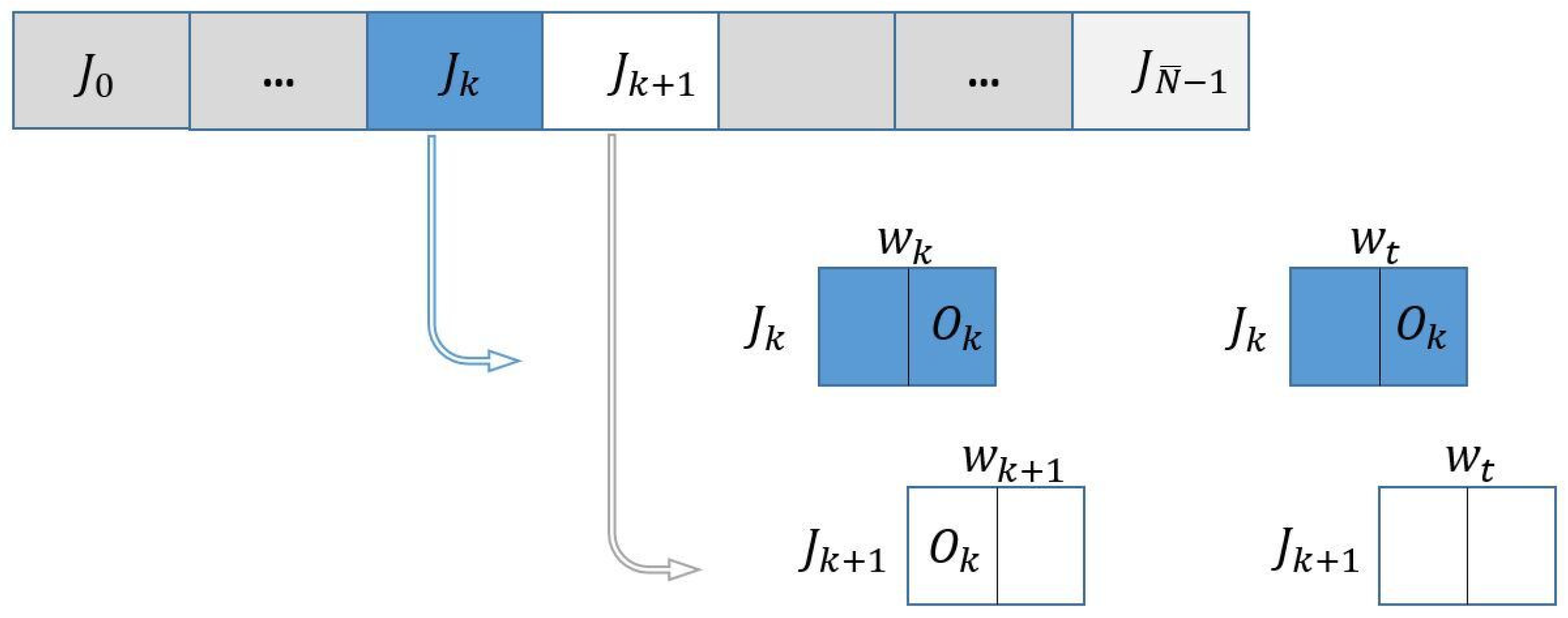
where $or={\displaystyle \frac{os}{2os+rs}}$. In this work, we have considered batches corresponding to the first case. Figure 1 schematically shows batches $J_k$ and $J_{k+1}$ at iterations k and $k+1$, respectively, and the overlapping parts in this case:

The stochastic loss value and gradient (22) are computed at the beginning (at $w_k$) and at the end of each iteration (at trial point $w_t$). In iteration $k+1$, these quantities have to be evaluated with respect to the sample subset represented by white rectangles only. In fact, the computations with respect to subset $O_k$ at $w_{k+1}$ depend on the acceptance status of $w_t$ at iteration k. In the case of acceptance, the loss function and gradient vector have been already computed at $w_t$; in the case of rejection, these quantities are set equal to those evaluated at $w_k$, with respect to subset $O_k$.

3. Results

We present in this section the results of extensive experimentation to assess the effectiveness of the two described stochastic QN algorithms at solving the unconstrained optimization problems arising from the training of DNNs to accomplish image classification tasks. The deep learning toolbox of MATLAB provides a framework for designing and implementing a deep neural network, to perform image classification tasks using a prescribed training algorithm. We have exploited the deep learning custom training loops of MATLAB (https://www.mathworks.com/help/deeplearning/deep-learning-custom-training-loops.html, accessed on 15 October 2020 ), to implement Algorithms 2 and 3 with half-overlapping subsampling. The implementation details of the two stochastic QN algorithms considered in this work, using the DL toolbox of MATLAB (https://it.mathworks.com/help/deeplearning/, accessed on 15 October 2020), are provided in https://github.com/MATHinDL/sL_QN_TR/, where all the codes employed to obtain the numerical results included in this paper are also available.

To find an optimal classification model by using a C-class dataset, the generic problem (1) is solved by employing the softmax cross-entropy function, defined as

$$L_i\left(w\right)=-\sum _{k=1}^C{\left(y_i\right)}_{k}log{\left(h(x_i;w)\right)}_k,$$

for $i=1,\dots ,N$. One of the most popular benchmarks for making informed decisions using data-driven approaches in DL is the MNIST dataset [41], as ${\left\{(x_i,y_i)\right\}}_{i=1}^{\mathrm{70,000}}$, consisting of handwritten gray-scale images of digits $x_i$ with $28\times 28$ pixels taking values in $[0,255]$ and its corresponding labels converted to one-hot vectors. Fashion-MNIST [42] is a variant of the original MNIST dataset, which shares the same image size and structure. Its images are assigned to fashion items (clothing) belonging also to 10 classes, but working with this dataset is more challenging than working with MNIST. The CIFAR-10 dataset [43] has 60,000 RGB images $x_i$ of $32\times 32$ pixels taking values in $[0,255]$ in 10 classes. Every single image of the MNIST and Fashion-MNIST datasets is $x_i\in {\mathbb{R}}^{28\times 28\times 1}$, while the one of CIFAR10 is $x_i\in {\mathbb{R}}^{32\times 32\times 3}$. In all the datasets, $\mathrm{10,000}$ of the images are set aside as a testing set during training.

In this work, inspired by LeNet-5—mainly used for character recognition tasks [44]—we have used a LeNet-like network with a shallow structure. We have also employed a modern ResNet-20 residual network [45], exploiting special skip connections (shortcuts) to avoid possible gradient vanishing that might happen due to its deep architecture. Finally, we also consider a self-built convolutional neural network (CNN) named ConvNet3FC2 with a larger number of parameters than the two previous networks. To analyze the effect of batch normalization [46] on the performance of the stochastic QN algorithms, we have considered also variants of the ResNet-20 and ConvNet3FC2 networks, named ResNet-20 (No BN) and ConvNet3FC2 (No BN), in which the batch normalization layers have been removed.

Table 1. Networks.

LeNet-like
Structure	$(Conv(5\times 5@20,1,0)/ReLu/MaxPool(2\times 2,2,0))$
	$(Conv(5\times 5@50,1,0)/ReLu/MaxPool(2\times 2,2,0))$
	$FC(500/ReLu)$
	$FC(C/Softmax)$
ResNet-20
Structure	$(Conv(3\times 3@16,1,1)/BN/ReLu)$
	$B_1\left\{\begin{array}{c}(Conv(3\times 3@16,1,1)/BN/ReLu)\hfill \\ (Conv(3\times 3@16,1,1)/BN)+addition\left(1\right)/Relu\hfill \end{array}\right.$
	$B_2\left\{\begin{array}{c}(Conv(3\times 3@16,1,1)/BN/ReLu)\hfill \\ (Conv(3\times 3@16,1,1)/BN)+addition\left(1\right)/Relu\hfill \end{array}\right.$
	$B_3\left\{\begin{array}{c}(Conv(3\times 3@16,1,1)/BN/ReLu)\hfill \\ (Conv(3\times 3@16,1,1)/BN)+addition\left(1\right)/Relu\hfill \end{array}\right.$
	$B_1\left\{\begin{array}{c}(Conv(3\times 3@32,2,1)/BN/ReLu)\hfill \\ (Conv(3\times 3@32,1,1)/BN)\hfill \\ (Conv(1\times 1@32,2,0)/BN)+addition\left(2\right)/Relu\hfill \end{array}\right.$
	$B_2\left\{\begin{array}{c}(Conv(3\times 3@32,1,1)/BN/ReLu)\hfill \\ (Conv(3\times 3@32,1,1)/BN)+addition\left(1\right)/Relu\hfill \end{array}\right.$
	$B_3\left\{\begin{array}{c}(Conv(3\times 3@32,1,1)/BN/ReLu)\hfill \\ (Conv(3\times 3@32,1,1)/BN)+addition\left(1\right)/Relu\hfill \end{array}\right.$
	$B_1\left\{\begin{array}{c}(Conv(3\times 3@64,2,1)/BN/ReLu)\hfill \\ (Conv(3\times 3@64,1,1)/BN)\hfill \\ (Conv(1\times 1@64,2,0)/BN)+addition\left(2\right)/Relu\hfill \end{array}\right.$
	$B_2\left\{\begin{array}{c}(Conv(3\times 3@64,1,1)/BN/ReLu)\hfill \\ (Conv(3\times 3@64,1,1)/BN)+addition\left(1\right)/Relu\hfill \end{array}\right.$
	$B_3\left\{\begin{array}{c}(Conv(3\times 3@64,1,1)/BN/ReLu)\hfill \\ \left(Conv(3\times 3@64,1,1)BN\right)+addition\left(1\right)/g.AvgPool/ReLu)\hfill \end{array}\right.$
	$FC(C/Softmax)$
ConvNet3FC2
Structure	$(Conv(5\times 5@32,1,2)/BN/ReLu/MaxPool(2\times 2,1,0))$
	$(Conv(5\times 5@32,1,2)/BN/ReLu/MaxPool(2\times 2,1,0))$
	$(Conv(5\times 5@64,1,2)/BN/ReLu/MaxPool(2\times 2,1,0))$
	$FC(64,/BN/ReLu)$
	$FC(C/Softmax)$

describes the networks’ architecture in detail. In this table, the syntax $(Conv(5\times 5@32,1,2)/BN/ReLu/MaxPool(2\times 2,1,0)))$ indicates a simple convolutional network (convnet) including a convolutional layer ($Conv$) using 32 filters of size $5\times 5$, stride 1, padding 2, followed by a batch normalization layer ($BN$), a nonlinear activation function ($ReLu$) and, finally, a max-pooling layer with a channel of size $2\times 2$, stride 1, and padding 0. The syntax $FC(C/Softmax)$ indicates a layer of C fully connected neurons followed by the softmax layer. Moreover, the syntax $addition\left(1\right)/Relu$ indicates the existence of an identity shortcut such that the output of a given block, say $B_1$ (or $B_2$ or $B_3$), is directly fed to the $addition$ layer and then to the ReLu layer while $addition\left(2\right)/Relu$ in a block shows the existence of a projection shortcut by which the output from the two first convnets is added to the output of the third convnet and then the output is passed through the ReLu layer.

Table 2. The total number of the networks’ trainable parameters (n).

	LeNet-5	ResNet-20	ResNet-20 (No BN)	ConvNet3FC2	ConvNet3FC2 (No BN)
MNIST	431,030	272,970	271,402	2,638,826	2,638,442
F.MNIST	431,030	272,970	271,402	2,638,826	2,638,442
CIFAR10	657,080	273,258	271,690	3,524,778	3,525,162

shows the total number of trainable parameters, n, for different image classification problems. We have compared algorithms sL-BFGS-TR and sL-SR1-TR in training tasks for these problems. We have used the hyperparameters $c=0.9$ and $\tau ={10}^{-2}$ in sL-BFGS-TR, $c_1=0.5$, $c_2=1.5$, $c={10}^{-6}$, and $\tau ={10}^{-8}$ in sL-SR1-TR, and ${\tau }_1={10}^{-4}$, ${\gamma }_0=1$, ${\tau }_2=0.1$, ${\tau }_3=0.75$, ${\eta }_3=0.8$, ${\eta }_2=0.5$, and ${\eta }_4=2$ in both ones. We have also used the same initial parameter $w_0\in {\mathbb{R}}^n$ by specifying the same seed to the MATLAB random number generator for both methods. All deep neural networks have been trained for at most 10 epochs, and training was terminated if $100\%$ accuracy was reached.

The accuracy is the ratio of the number of correct predictions to the number of total predictions. In our study, we report the accuracy in percentage and overall loss values for both the train and the test datasets. Following prior published works in the optimization community (see, e.g., [28]) we use the whole testing set as the validation set: that is, at the end of each iteration of the training phase (after the network parameters have been updated) the prediction capability of the recently updated network is evaluated, using all the samples of the test dataset. The computed value is the measured testing accuracy corresponding to iteration k. Consequently, we report accuracy and loss across epochs for both the training samples and the unseen samples of the validation set (=the test set) during the training phase.

To facilitate visualization, we plot the measurement under evaluation versus epochs, using a determined frequency of display, which is reported at the top of the figures. Display frequency values larger than one indicate the number of iterations that are not reported, while all the iterations are considered if the display frequency is one. All the figures report the results of a single run; see also the additional experiments in the Supplementary Material.

We have performed extensive testing to analyze different aspects that may influence the performance of the two considered stochastic QN algorithms: mainly, the limited memory parameter and the batch size. We have also compared the performance of both algorithms from the point of view of CPU time. Finally, we have provided a comparison with first- and second-order methods. All experiments were performed on a Ubuntu Linux server virtual machine with 32 CPUs and 128 GB RAM.

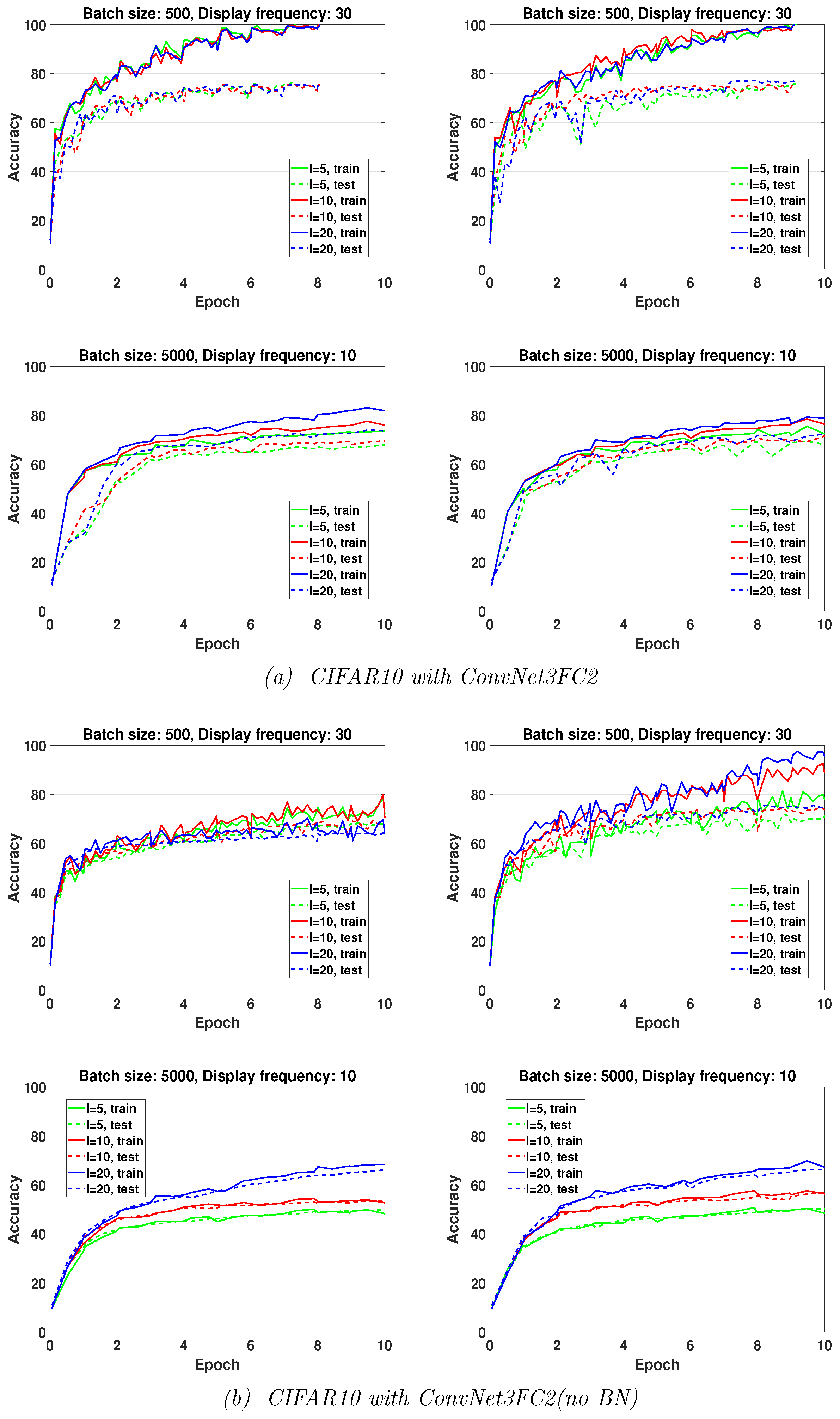
3.1. Influence of the Limited Memory Parameter

The results reported in Figure 2 illustrate the effect of the limited memory parameter value ($l=5,10$ and 20) on the accuracy achieved by the two stochastic QN algorithms in training ConvNet3FC2 on CIFAR10 within a fixed number of epochs. As is clearly shown in this figure, in particular for ConvNet3FC2 (No BN), the effect of the limited memory parameter is more pronounced when large batches are used ($bs=5000$). For large batch sizes, the larger the value of l, the higher the accuracy. No remarkable differences in the behavior of both algorithms with a small batch size ($bs=500$) are observed. It seems that incorporating more recently computed curvature vectors (i.e., larger l) does not increase the efficiency of the algorithms in training DNNs with BN layers, while it does when BN layers are removed. Finally, we remark that we have found that using larger values of l ($l\ge 30$) is not helpful, having led to higher over-fitting in some of our experiments.

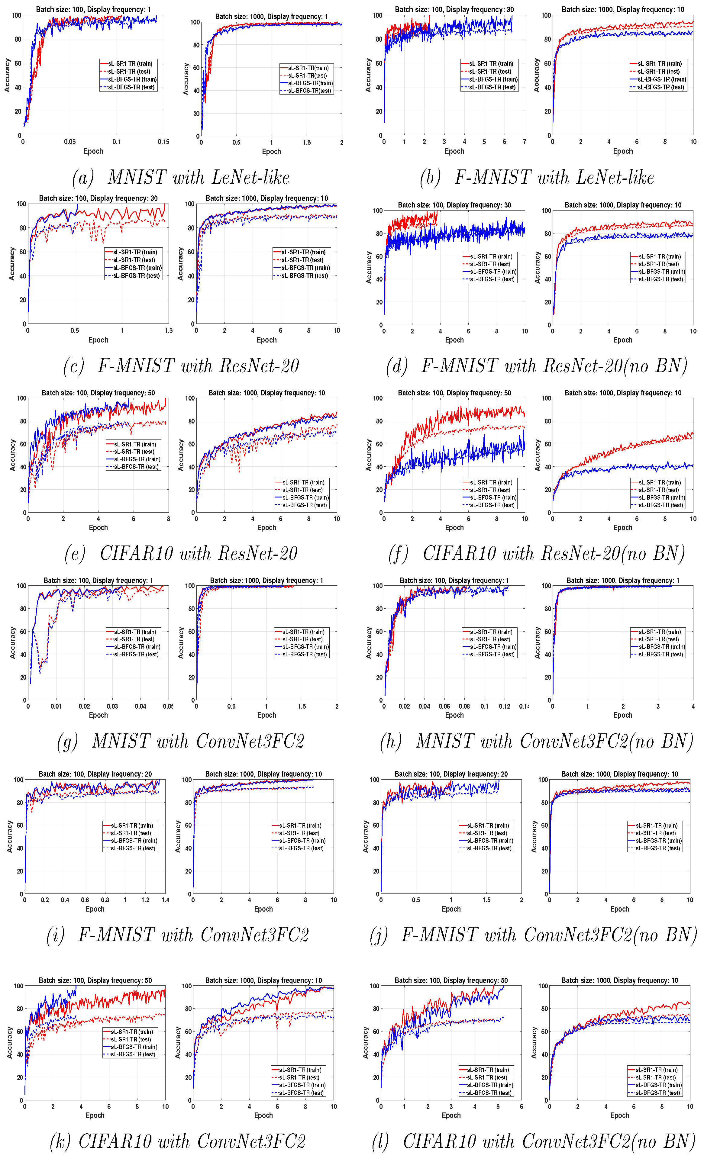
3.2. Influence of the Batch Size

In this subsection, we analyze the effect of the batch size on the performance of the two considered sQN methods, while keeping fixed the limited memory parameter $l=20$. We have considered different values of the batch size ($bs$) in $\{100,500,1000,5000\}$ or, equivalently, overlap size ($os$) in $\{50,250,500,2500\}$ for all the problems and all the considered DNNs. Based on Figure 3, the general conclusion is that when training the networks for a fixed number of epochs, the achieved accuracy decreases when the batch size increases. This is due to the reduction in the number of parameter updates. We have summarized in

Table 3. Summary of the best sQN approach for each combination problem/network architecture.

	LeNet-5	ResNet-20	ResNet-20 (No BN)	ConvNet3FC2	ConvNet3FC2 (No BN)
MNIST	sL-SR1-TR	both	sL-SR1-TR	both	both
F.MNIST	sL-SR1-TR	both	sL-SR1-TR	both	sL-SR1-TR
CIFAR10	sL-SR1-TR	sL-BFGS-TR	sL-SR1-TR	sL-BFGS-TR	sL-SR1-TR

the relative superiority of one of the two stochastic QN algorithms over the other for all problems. With “both”, we indicate that both algorithms display similar behavior. From the results reported in Table 3, we conclude that sL-SR1-TR performs better than sL-BFGS-TR for training networks without BN layers, while both QN updates exhibit comparable performances when used for training networks with BN layers. More detailed comments for each DNN are given below.

3.2.1. LeNet-like

The results on top of Figure 3 show that both the algorithms perform well, in training LeNet-like within 10 epochs to classify MNIST and Fashion-MNIST datasets, respectively. Specifically, sL-SR1-TR provides better classification accuracy than sL-BFGS-TR.

3.2.2. ResNet-20

Figure 3 shows that the classification accuracy on Fashion-MNIST increases when using ResNet-20 instead of LeNet-like, as expected. Regarding the performance of the two algorithms of interest, both algorithms exhibit comparable performances when BN is used. Nevertheless, we point out the fact that sL-BFGS-TR using $bs=100$ achieves higher accuracy than sL-SR1-TR, in less time. This comes with some awkward oscillations in the testing curves. We attribute these oscillations to a sort of inconsistency between the updated parameters and the normalized features of the testing set samples. This is due to the fact that the inference step by testing samples is done using the updated parameters and the features that are normalized by the most recently computed mean and variance moving average values obtained by the batch normalization layers in the training phase [46]. The numerical results on ResNet-20 without the BN layers confirm this assumption can be true. These results also show that sL-SR1-TR performs better than sL-BFGS-TR in this case. Note that the experiments on LeNet-like and ResNet-20 with and without BN layers show that sL-SR1-TR performs better than sL-BFGS-TR when batch normalization is not used, but, as can be clearly seen from the results, the elimination of the BN layers causes a detriment to all the methods’ performances.

3.2.3. ConvNet3FC2

Figure 3 shows that sL-BFGS-TR still produces better testing/training accuracy than sL-SR1-TR on CIFAR10, while both algorithms behave similarly on the MNIST and Fashion-MNIST datasets. In addition, sL-BFGS-TR with $bs=100$ within 10 epochs achieves the highest accuracy faster than sL-SR1-TR (see Figure 3k).

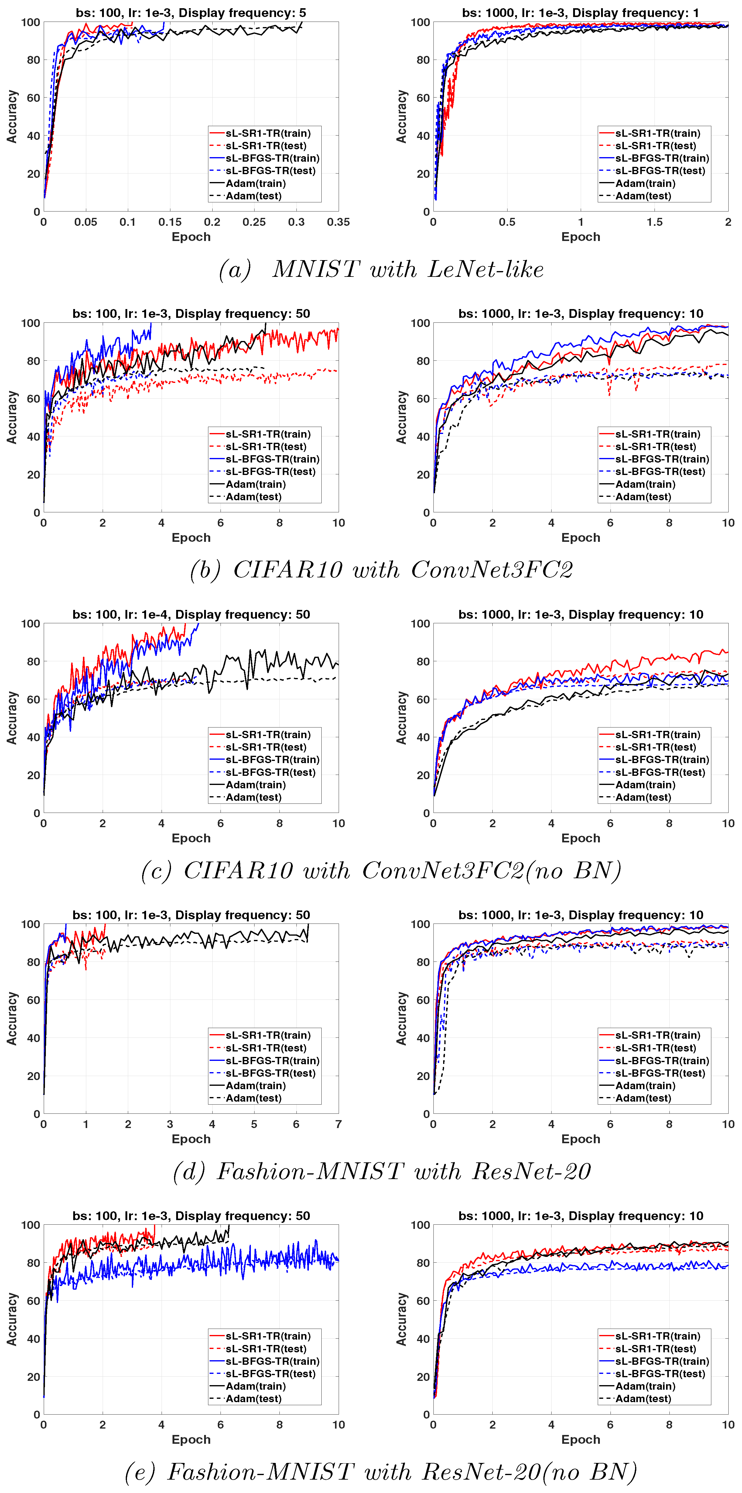
3.3. Comparison with Adam Optimizer

Adaptive moment estimation (Adam) [7] is a popular efficient first-order optimizer used in DL. Due to the high sensitivity of Adam to the value of its hyperparameters, it is usually used after the determination of near-optimal values through grid searching strategies, which is a very time-consuming task. It is worth noting that sL-QN-TR approaches do not require step-length tuning, and this particular experiment offers a comparison to optimized Adam. To compare sL-BFGS-TR and sL-SR1-TR to Adam, we have performed a grid search on learning rates and batch sizes, to select the best value of Adam’s hyperparameters. We have considered learning rates values in $\{{10}^{-5},{10}^{-4},{10}^{-3},{10}^{-2},{10}^{-1},1\}$ and batch size in $\{100,500,1000,5000\}$, and we have selected the pair of values that allows Adam to achieve the highest testing accuracy. The gradient and squared gradient decay factors are set as ${\beta }_1=0.9$ and ${\beta }_2=0.999$, respectively. The small constant for preventing divide-by-zero errors is set to ${10}^{-8}$.

Figure 4 illustrates the results obtained with the two considered sQN algorithms and the tuned Adam. We have analyzed which algorithm achieves the highest training accuracy within, at most, 10 epochs for different batch sizes. In networks using BN layers, all methods achieve comparable training and testing accuracy within 10 epochs with $bs=1000$. However, this cannot be generally observed when $bs=100$. The figure shows that tuned Adam provides higher testing accuracy than sL-SR1-TR. Nevertheless, sL-BFGS-TR is still faster at achieving the highest training accuracy, as we also previously observed. It also provides testing accuracy comparable to tuned Adam. On the other hand, for networks without BN layers, sL-SR1-TR is the clear winner.

A final remark is that Adam’s performance seems to be more negatively affected by large minibatch size than QN methods. For this reason, QN methods can increase their advantage over Adam when using large batch sizes to enhance the parallel efficiency of distributed implementations.

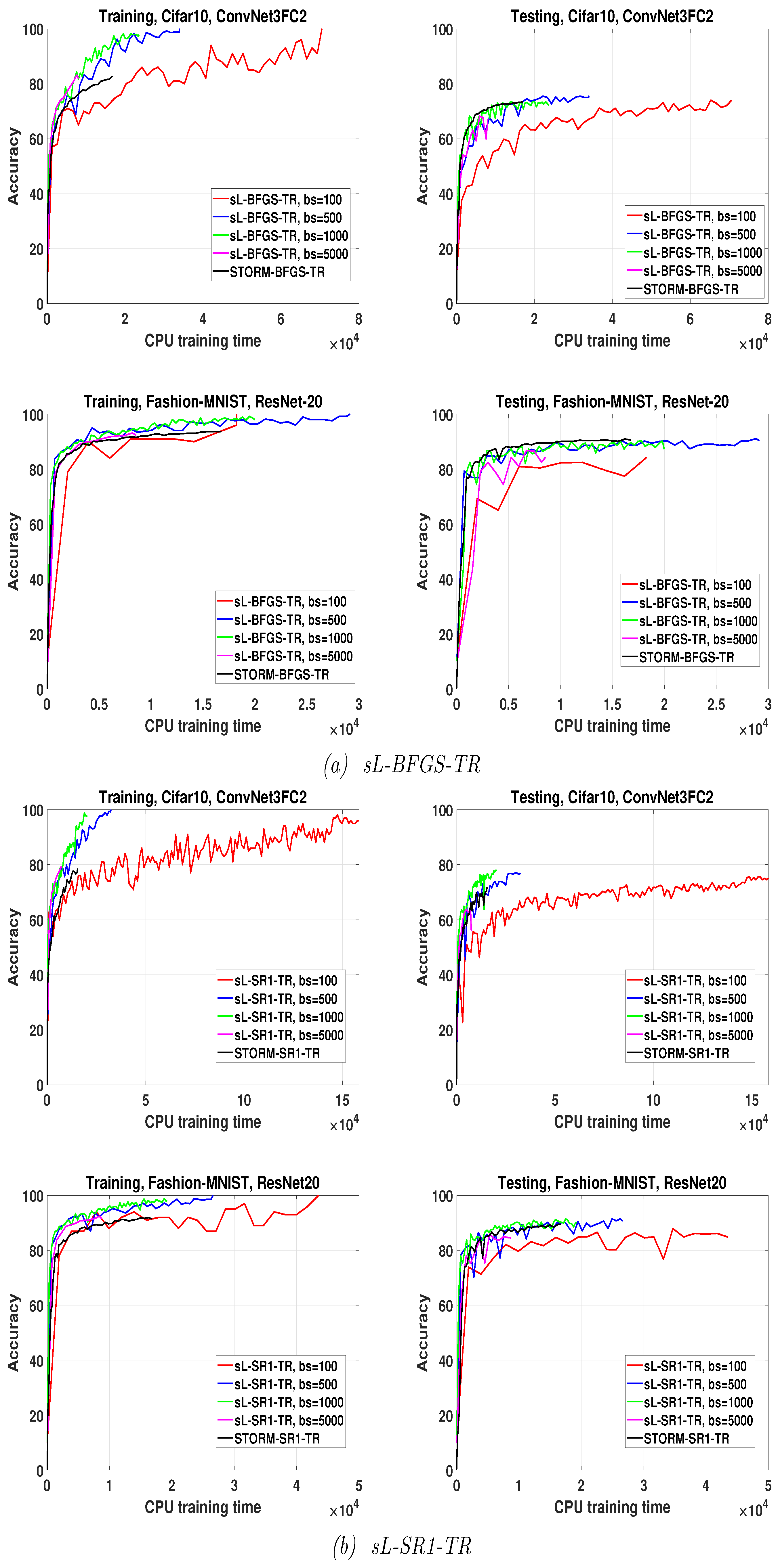
3.4. Comparison with STORM

We have performed a comparison between our sQN training algorithms and the algorithm STORM (Algorithm 5 in [47]). STORM relies on an adaptive batching strategy aimed at avoiding inaccurate stochastic function evaluations in the TR framework. Note that the real reduction of the objective function is not guaranteed in a stochastic-trust-region approach. In [32,47], the authors claim that if the stochastic functions are sufficiently accurate, this will increase the number of true successful iterations. Therefore, they considered a progressive sampling strategy with sample size

$$b_k=min(N,max(b_0·k+b_1,\lceil \frac{1}{{{\delta }_k}^2}\rceil )),$$

where ${\delta }_k$ is the trust region radius at iteration k, N is the total number of samples, and $b_0,b_1$ are $b_0=100,b_1=32\times 32\times 3$ for CIFAR10, and $b_1=28\times 28\times 1$ for Fashion-MNIST.

We have applied STORM with both L-SR1 and L-BFGS updates. We have compared the performances of the sL-SR1-TR and sL-BFGS-TR algorithms employing different overlapping batch sizes running for 10 epochs with the performance provided by STORM with progressive batch size $b_k$ running for 50 epochs. We allowed STORM to execute for more epochs, i.e., 50 epochs, since, due to its progressive sampling behavior it passed 10 epochs very rapidly. The largest batch size reached by STORM within this number of epochs is near $b_k=\mathrm{25,000}$ (i.e., 50 percent of the total number of training samples).

The results of this experiment are summarized in Figure 5. In both Fashion-MNIST and CIFAR10 problems, the algorithms with $bs=500$ and $bs=1000$ produce comparable or higher final accuracy than STORM at the end of their respective training phases. Even if we set a fixed budget of time corresponding to the one needed by STORM to perform 50 epochs, sL-QN-TR algorithms with $bs=500$ and $bs=1000$ provide comparable or higher accuracy. The results corresponding to the smallest and largest batch sizes need a separate discussion. When $bs=100$, the stochastic QN algorithms are not better than STORM with any fixed budget of time; however, they provide higher final training accuracy and testing accuracy, except for the Fashion-MNIST problem on ResNet-20 trained by sL-BFGS-TR.

By contrast, when $bs=5000$, sL-BFGS-TR algorithms produce higher or comparable training accuracy but not a testing accuracy comparable to the one provided by STORM. This seems quite logical, as using such a large batch size causes the algorithms to perform a small number of iterations and then to update the parameter vector only a few times; allowing longer training time or more epochs can compensate for this lower accuracy. Finally, this experiment shows also that the sL-BFGS-TR algorithm with $bs=5000$ yields higher accuracy within less time than that obtained when $bs=100$ is used.

4. Conclusions

We have studied stochastic QN methods for training deep neural networks. We have considered both L-SR1 and L-BFGS updates in a stochastic setting in a trust region framework. Extensive experimental work—including the effect of batch normalization (BN), the limited memory parameter, the sampling strategy, and batch size—has been reported and discussed. Our experiments show that BN is a key factor in the performance of stochastic QN algorithms and that sL-BFGS-TR behaves comparably to or slightly better than sL-SR1-TR when BN layers are used, while sL-SR1-TR performs better in networks without BN layers. This behavior is in accordance with the property of L-SR1 updates allowing for indefinite Hessian approximations in non-convex optimization. However, the exact reason for the different behavior of the two stochastic QN algorithms with networks not employing BN layers is not completely clear and would deserve further investigation.

The reported experimental results have illustrated that employing larger batch sizes within a fixed number of epochs produces lower training accuracy, which can be recovered by longer training. Regarding training time, our results have also shown a slight superiority in the accuracy reached by both algorithms when larger batch sizes are used within a fixed budget of time. This suggests the use of large batch sizes also in view of the parallelization of the algorithms.

The proposed sQN algorithms, with the overlapping fixed-size sampling strategy, revealed to be more efficient than the adaptive progressive batching algorithm STORM, which naturally incorporates a variance reduction technique.

Finally, our results show that sQN methods are efficient in practice and, in some instances, outperform tuned Adam. We believe that this contribution fills a gap concerning the real performance of the SR1 and BFGS updates in realistic large-size DNNs, and it is expected to help steer the researchers in this field towards the option of the proper quasi-Newton method.