Neural Network-Enhanced Fault Diagnosis of Robot Joints

Abstract

Industrial robots play an indispensable role in flexible production lines, and the faults caused by degradation of equipment, motors, mechanical system joints, and even task diversity affect the efficiency of production lines and product quality. Aiming to achieve high-precision multiple size of fault diagnosis of robotic arms, this study presents a back propagation (BP) multiclassification neural network-based method for robotic arm fault diagnosis by taking feature fusion of position, attitude and acceleration of UR10 robotic arm end-effector to establish the database for neural network training. The new algorithm achieves an accuracy above 95% for fault diagnosis of each joint, and a diagnostic accuracy of up to 0.1 degree. It should be noted that the fault diagnosis algorithm can detect faults effectively in time, while avoiding complex mathematical operations.

1. Introduction

With the wide application of informatisation, digitalisation and intelligentisation technologies, the automation level of manufacturing enterprises has been significantly improved, and flexible production lines aiming at rapid automated machining of multi-species precision parts have been proposed, which is of great significance and value for the transformation and upgrading of the manufacturing enterprises’ production methods, equipment manufacturing capabilities and product performance [1]. In the processing of flexible production line, it is particularly important to maintain the product quality and quantity, and improve production efficiency, which directly affect the production efficiency and economic benefits of enterprises [2]. In the past decades, a large amount of research has been devoted to production systems, focusing on modelling, performance analysis, bottleneck identification, lean design, product quality inspection and production control of production systems [3]. However, these macro-analyses are based on industrial robots, as the most important players in the flexible production line, with their advantages of high efficiency, multi-functionality, and high operational accuracy as an indispensable part of the flexible production line, and the accuracy of the robot arm’s movement trajectory is directly related to the product quality, production efficiency, and economic benefits of the entire flexible production system [4].

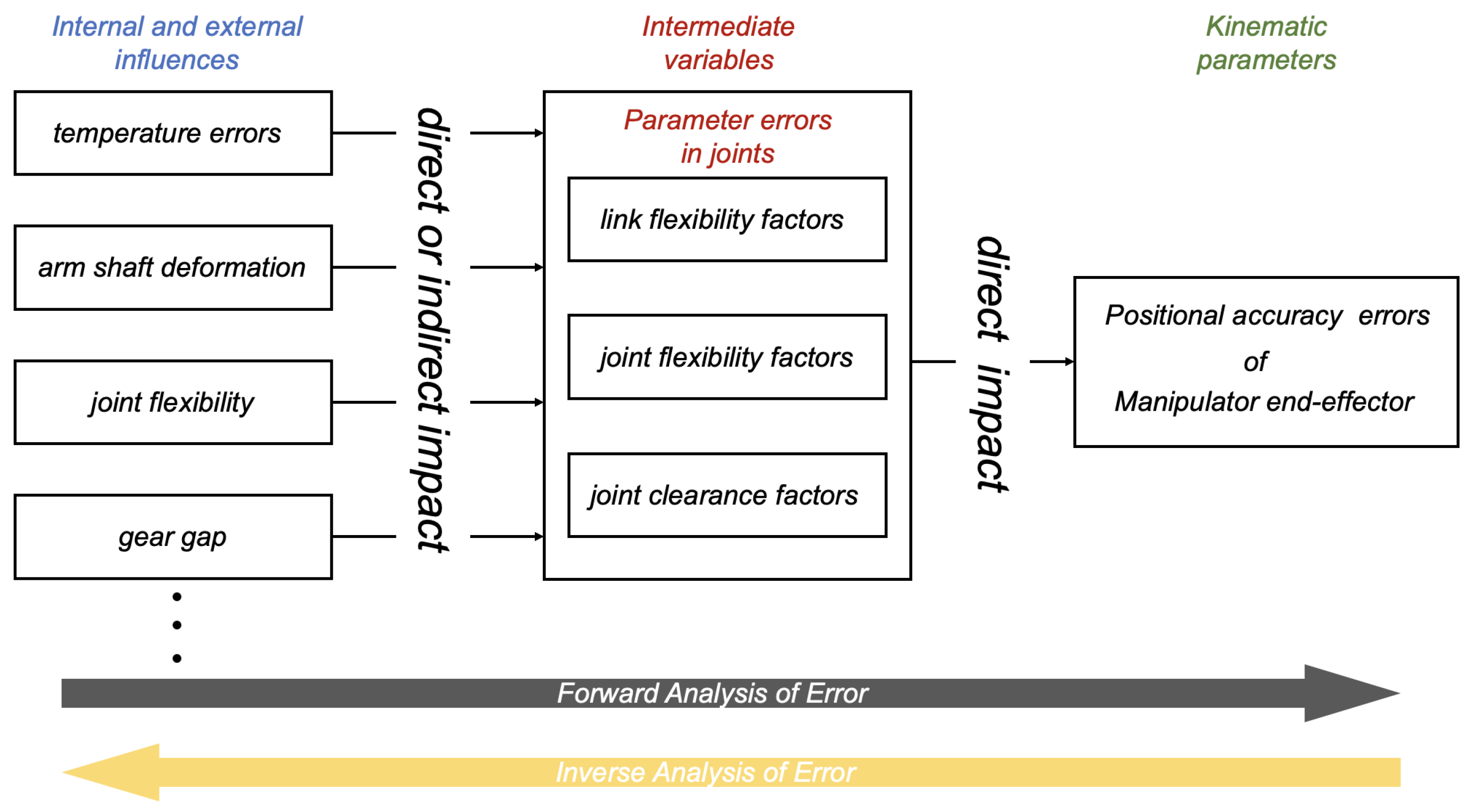
The kinematic accuracy of the robot is the basis for the accurate execution of the robot’s movements, and kinematic reliability is a key indicator for evaluating the kinematic performance of the robot. In [5,6], the end-effector of manipulator positional accuracy errors mainly include structural and joint kinematic parameter errors, such as temperature errors, arm shaft deformation, joint flexibility, gear clearance, wear, etc., which ultimately affect the robot kinematic parameters directly or indirectly. In [7], the reliability of motion accuracy is defined and factors affecting motion reliability represented by link flexibility factors, joint flexibility factors and joint clearance factors of the manipulator are proposed. These three factors are considered to be intermediate to the various internal and external influences on the kinematic parameters of the robot. In other words, any influencing factor first affects the linkage flexibility factor, the joint flexibility factor and the joint clearance factor, and then affects the kinematic parameters, leading to a decrease in the reliability of the robot arm. Figure 1 shows the forward and inverse fault analysis processes.

In this context, fault diagnosis is particularly important, the specific joint in question is known by analysing the error in the end-effector of the manipulator, and then the three parameters of that joint are calculated and compared to eliminate the influencing factors and improve the reliability of the motion accuracy. And, based on the back propagation neural network and the trajectory of the robotic arm, it is possible to diagnose faults in specific joints.

The aim of this research is to develop and validate a neural network-based robotic arm joint fault diagnosis system by monitoring the position and attitude data of end-effector in real time, in order to achieve accurate identification and analysis of robotic arm joint faults so as to improve the operational efficiency and safety of the robotic arm. Several research questions exist in neural network-based fault diagnosis of robotic arm joints:

• How to use neural networks effectively to diagnose joint failures in robotic arms;
• How to build the database needed for neural network training, validation and testing;
• How to inject faults and enable neural networks to predict faulty joints;
• What metrics to select to evaluate the performance of neural networks.

In order to achieve the aim and deal with these problems so that the neural network can effectively accurately diagnose line-of-sight faults, the objectives of this study are briefly explained as follows:

• Feature sampling of the trajectories generated by the computation of the forward motion of the robotic arm and the creation of a database after data processing;
• Development and validation of a neural network classification based algorithm for real-time diagnosis of robotic arm joint faults;
• Identification of the mechanism to inject faults and enable neural networks to predict faulty joints;
• The selection of metrics to evaluate the performance of neural networks.

Ref. [8] proposes the use of embedded machine vision and observers to aid diagnosis. The specific method is to identify the position of the end-effector by means of a stereo camera, which has the advantages of simple implementation, high accuracy of typical fault detection, and elimination of the need to use additional sensors. The advantages are simple to implement and high accuracy of typical fault detection. But the disadvantages are that dual stereo cameras increase the cost and are environmentally demanding, and it can not be determined what kind of faults occur in which specific part.

A more popular approach is to design a variety of observers for fault diagnosis based on robot characteristics. Wu et al. [9] used a learning observer to diagnose robotic sensor faults: firstly, the dynamics model of the robotic arm was transformed into a state-space model, auxiliary state equations were constructed, sensor faults were transformed into actuator faults, and then time-varying faults were accurately estimated based on the advantages of the learning observer, which was computed through the LMI technique, a sliding mode fault tolerant controller is then designed to enable the robotic arm system to accurately track the desired trajectory. Ref. [10] provides a new approach to fault detection despite the failure of either sensors or actuators. The object of the study is the manipulators, which are modelled by a class of nonlinear systems with Lipschitz-like nonlinearities and modelling uncertainties, constructed in situations where actuator and sensor failures occur simultaneously leading to corrupted feedback information from the fault detection and isolation and where the residual signals may be sensitive to both actuator failures and sensor failures. Nonlinear adaptive observer that converges exponentially to a pre-specified range of estimation errors. These two studies have the advantage of being able to compensate for faults, but they do not allow precise identification of the cause of the fault. In contrast, fault diagnosis of robots based on BP neural networks perfectly overcomes these disadvantages.

Ref. [11] proposed a robotic arm fault diagnosis based on a decision tree. While the derivation of the eigenvectors used in the decision tree is complicated, firstly, the original vibration signals are separated by the empirical modal decomposition (EMD) algorithm to obtain the intrinsic modal function (IMF). Then, the envelopes of the IMF are obtained by Hilbert transform and the spectral energy of each envelope is calculated. Finally, the eigenvectors representing the envelope spectral energies are selected and combined to form the signal. Although the results of fault diagnosis are acceptable, the process is computationally and time intensive, and not real-time, so it is likely to have fewer applications in industry. The study is innovative, but the stability needs to be improved, and the diagnostic errors are vague, such as failure to approach the grasping position, and do not diagnose the exact cause of the failure. Ref. [12] proposes a neural network-based fault diagnosis and fault-tolerant control method for mobile robot control where, firstly, the neural network state observer is trained by a real nonlinear control system, and then the faults in the control system are detected and judged based on the residuals between the actual system output and the neural network observer output. This approach is common to this study in that both identify errors by comparing theoretical and practical results, but the disadvantage is that fault identification based on non-linear models requires more calculations and has a certain delay in identifying faults in real time. There is a similar study that collects the trajectories of different faulty robotic arm movements to build a database and train it with the network to finally achieve fault classification [2]. The disadvantage of this research is that the results obtained by fault classification with a single feature have low credibility and it does not give the possibilities for industrial applications, i.e., it does not separate faulty situations from non-faulty situations, which becomes a disadvantage of the application of this research.

In this paper, a BP classification neural network-based fault diagnosis method for robotic arms is developed with the goal of multi-stage and high-precision fault diagnosis of robotic arms, with robotic arm motion as the object of study. The neural network is fully capable of automatically weighting and classifying data with different characteristics by virtue of its ability to learn data samples to approximate the mapping relationship describing a nonlinear system, and the algorithmic feature of weight updating. The object of this study is the UR10 robotic arm [13], which has become one of the most widely used industrial robots due to its collaborative nature, ease of programming and flexibility.

The rest of the study includes the following sections. Section 2 gives the forward kinematics algorithm for the generation of trajectories by the robotic arm and the neural network algorithm used for classification. Section 3 describes the methods and principles of training the network with data-sets consisting of different features. Section 4 demonstrates the diagnosis procedure with simulation operations, where the performance of the classifier is evaluated by more metrics. Section 5 summarises the study.

2. Algorithm Analysis for BP Classification Neural Network

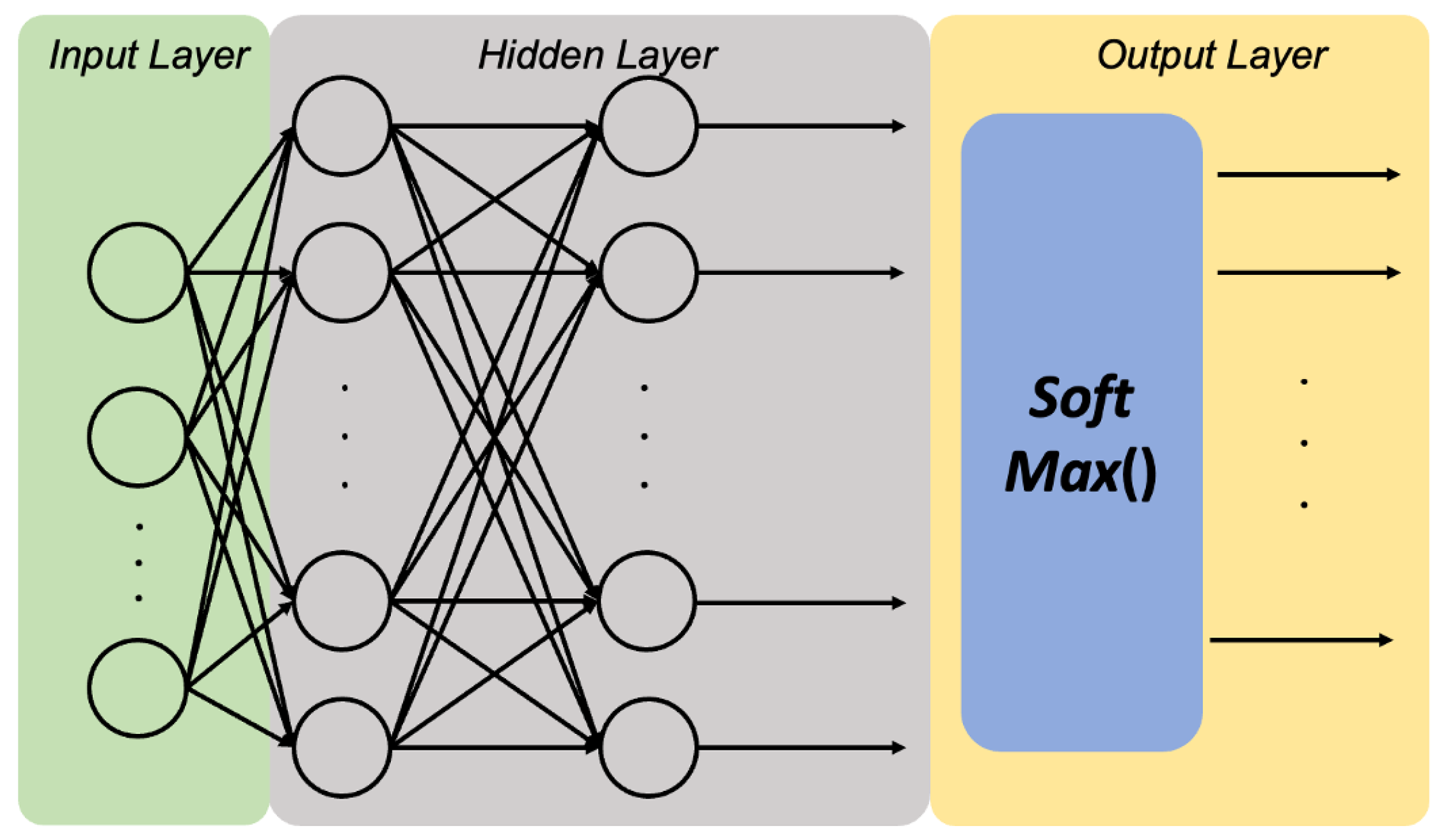
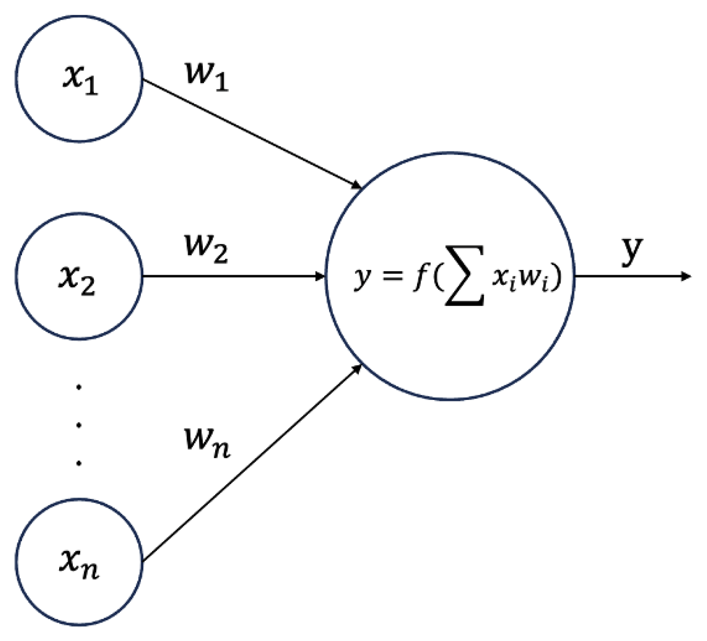
A neural network, as one of the most popular artificial intelligence algorithms, can be divided into classification and regression neural network according to their function. The basic forward propagation algorithm of these two are the same, as shown in Figure 2.

As shown in the figure, x represents the output of the input layer or the previous layer of neurons, and w represents the weights connecting the two neurons to each other, both of which, when subjected to linear regression as the independent variable of the activation function, are outputted to become the inputs or direct outputs of the next layer of neurons. Activation functions as nonlinear tools are directly responsible for neural networks to handle complex nonlinear model mapping. In the process of network construction, the activation function used in this research is sigmoid, which can map any real number to the interval (0,1), so its output can be interpreted as a probability, which is also the most commonly used activation function in classification problems in machine learning.

The essence of neural network training is to find the lowest loss through the gradient descent and in the process of constantly updating the weights [14]. The biggest difference between classification neural networks and regression neural networks is the activation function of the neurons in the output layer, which is shown in Figure 3.

The former is transformed nonlinearly by SoftMax as the activation function, which is commonly used in multiple classification problems in machine learning and deep learning, and it serves to transform a set of linear scores into a set of probability distributions. This process can be understood as a normalised exponential function. Specifically, let y be an n-dimensional real vector (in neural networks, this is usually the output of the last layer, also called logits or scores), and the SoftMax function is defined as:

$$softmax{\left(y\right)}_i=\frac{e^{y_i}}{{\sum }_{j=1}^n{e}^{y_j}}$$

(1)

Through this transformation, the SoftMax function transforms each output into a real number between 0 and 1, and the sum of all these transformed real numbers is 1, so they can be interpreted as a probability distribution. When performing a multiclassification problem, the SoftMax operation preserves the order between its parameters, so we do not need to compute SoftMax to determine which class has been assigned the highest probability; the class with the highest SoftMax value is usually used as the prediction, and that value is interpreted as the output of the model as a specific class by the Onehot encoding, which is used to represent the class labels. The encoding form is an q-order unitary matrix, with q denoting the number of labels (categories) to be classified [15].

In addition to the difference in the output layer activation function, another difference in classification neural networks lies in the loss function. As we mentioned earlier, the SoftMax function is used to convert the output of the neural network into a probability distribution, which can be viewed as the predicted probability of our model for each category. In this case, our goal is to make the model’s predicted probability distribution as close as possible to the true label distribution by tuning the model parameters. For a given data point, its true label distribution can be represented by one-hot coding. Thus, our task becomes maximising the model’s predictive probability for the true labels, i.e., maximising the likelihood function [16].

$$P(\mathbf{Y}\mid \mathbf{X})=\prod _{i=1}^{n}P\left({\mathbf{y}}^{\left(i\right)}\mid {\mathbf{x}}^{\left(i\right)}\right)$$

(2)

However, directly maximising the likelihood function can be numerically computationally problematic, e.g., overflow or underflow may be encountered. To avoid these problems, we usually take the logarithm of the likelihood function and convert the maximised likelihood function to minimise the negative log-likelihood.

$$-logP(\mathbf{Y}\mid \mathbf{X})=\sum _{i=1}^n-logP\left({\mathbf{y}}^{\left(i\right)}\mid {\mathbf{x}}^{\left(i\right)}\right)=\sum _{i=1}^{n}l\left({\mathbf{y}}^{\left(i\right)},{\widehat{\mathbf{y}}}^{\left(i\right)}\right)$$

(3)

In this context, the cross-entropy loss function is the negative log-likelihood function [17]:

$$l(\mathbf{y},\widehat{\mathbf{y}})=-\sum _{j=1}^q{y}_{j}log{\widehat{y}}_j$$

(4)

The cross-entropy loss function can be thought of as a measure between the predicted probability distribution and the true labelled probability distribution [18]. Ideally, we would like the model’s predicted probability distribution to exactly match the true label distribution. However, in reality, the model’s prediction may have some deviation. The cross-entropy loss function is one way to measure this bias, and it is a continuous metric that takes into account the probability of the model’s predictions. The greater the probability that the model predicts the correct category, the smaller the cross-entropy loss; conversely, if the model predicts the correct category with less probability, the greater the cross-entropy loss.

At the same time, accuracy is also one of the most important indicators of classifier performance:

$$\mathrm{Accuracy}=(\mathrm{Number}\mathrm{of}\mathrm{correct}\mathrm{predictions})/(\mathrm{Total}\mathrm{number}\mathrm{of}\mathrm{predictions})$$

(5)

Meanwhile, the ROC-AUC graph and confusion matrix are also important metrics for evaluation of the classification neural network, which can provide more information compared to the cross-entropy loss and accuracy.

3. Diagnosis Framework

3.1. Methodology Overview

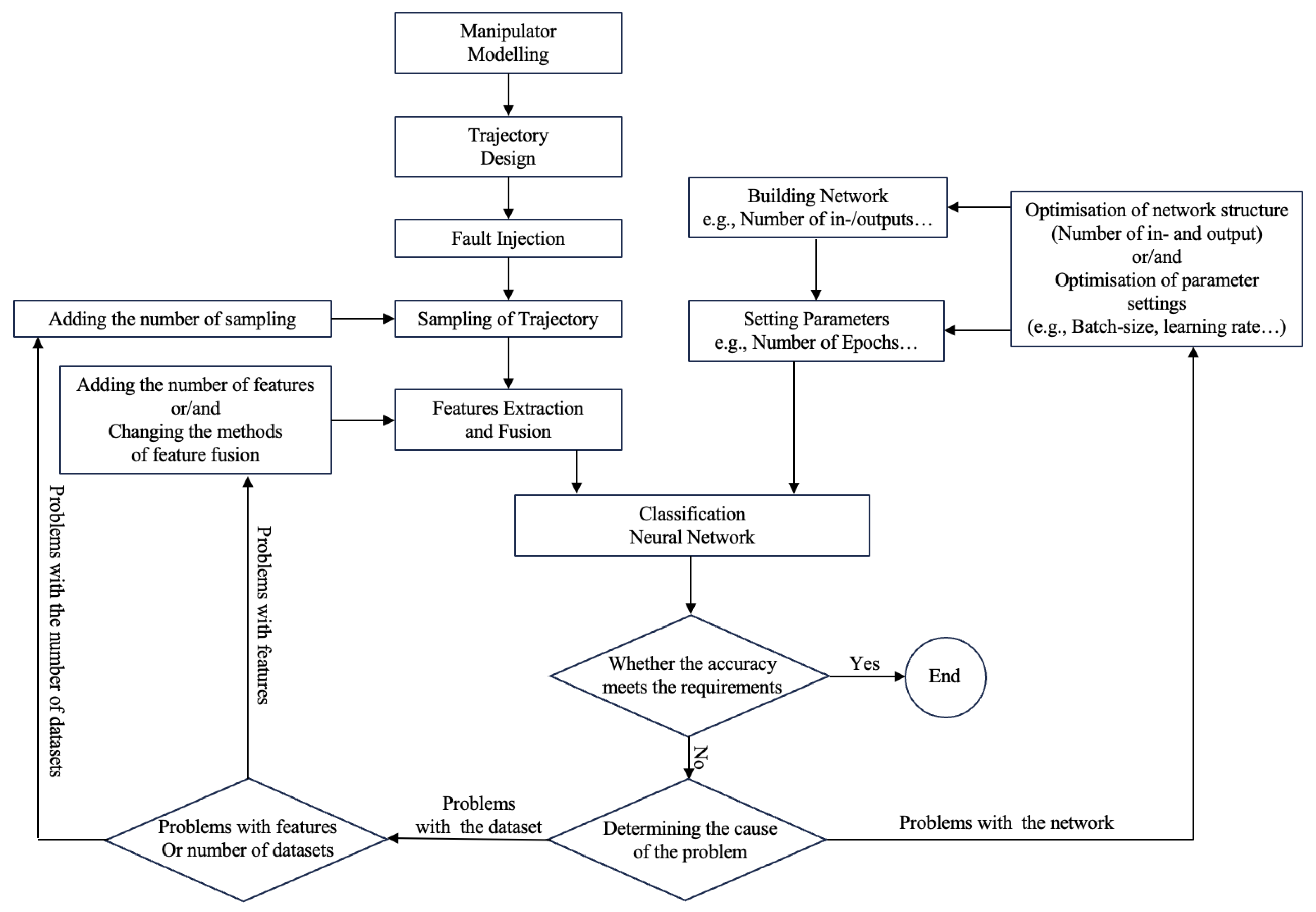
The aim of this study is to develop a procedure for the fault diagnosis of the UR10 robotic arm based on a BP neural network, which is capable of distinguishing different trajectories from measured data, so that the features are continuously extracted and fused to make the database optimised continuously recursively. The main idea and methodology of this research is shown in Figure 4.

First of all, the neural network as a classifier is the core of this research, the data obtained through the positive motion algorithm of the robotic arm is captured and fused, and will be used as a dataset for the training and testing of the neural network. It is generally considered that the classification accuracy of the neural network is acceptable above 95%; if this accuracy is not reached, firstly, the reason of the classifier itself or the dataset would be judged; if it is the problem of the dataset, we will check the trajectory of the robotic arm generation, the data collection and the fusion to see whether the problem occurs, and then, after checking the correctness of the network, the network’s structure and the various hyper-parameters would be adjusted to optimise it. In fact, the two are highly correlated; in addition to this, since the object of study in this experiment is simulated on software and all joint faults are injected artificially, there will be no problems such as mechanical wear and tear. There will be no factors such as mechanical wear and deformation to interfere with the results. To compare with similar research [2], the advantages of this research is that the database generated by multiple features of the forward kinematics, which could improve the diagnostic accuracy and classification and, in this way, the features and data fusion methods can be updated according to practical needs.

3.2. Establishment of the Database

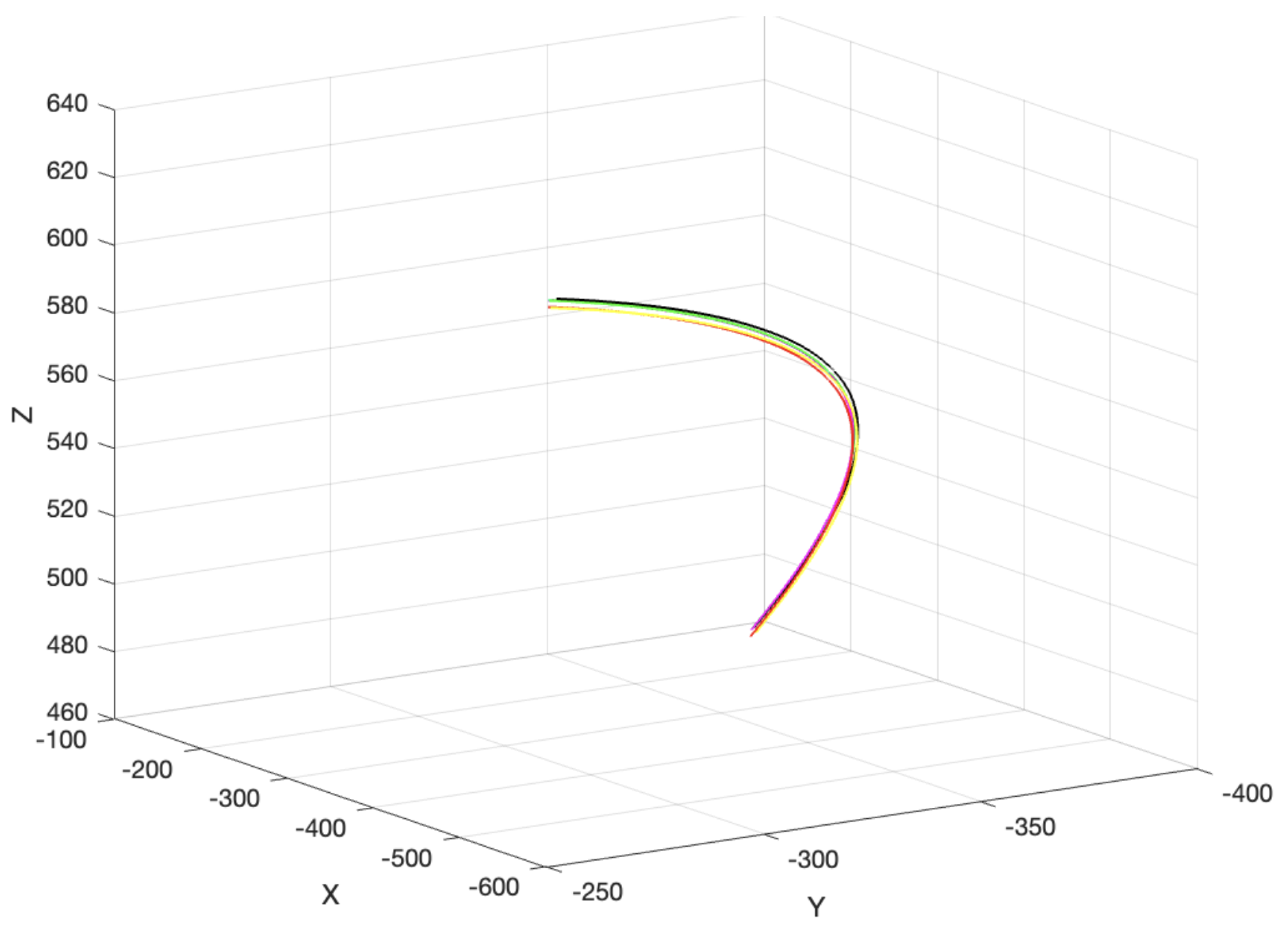
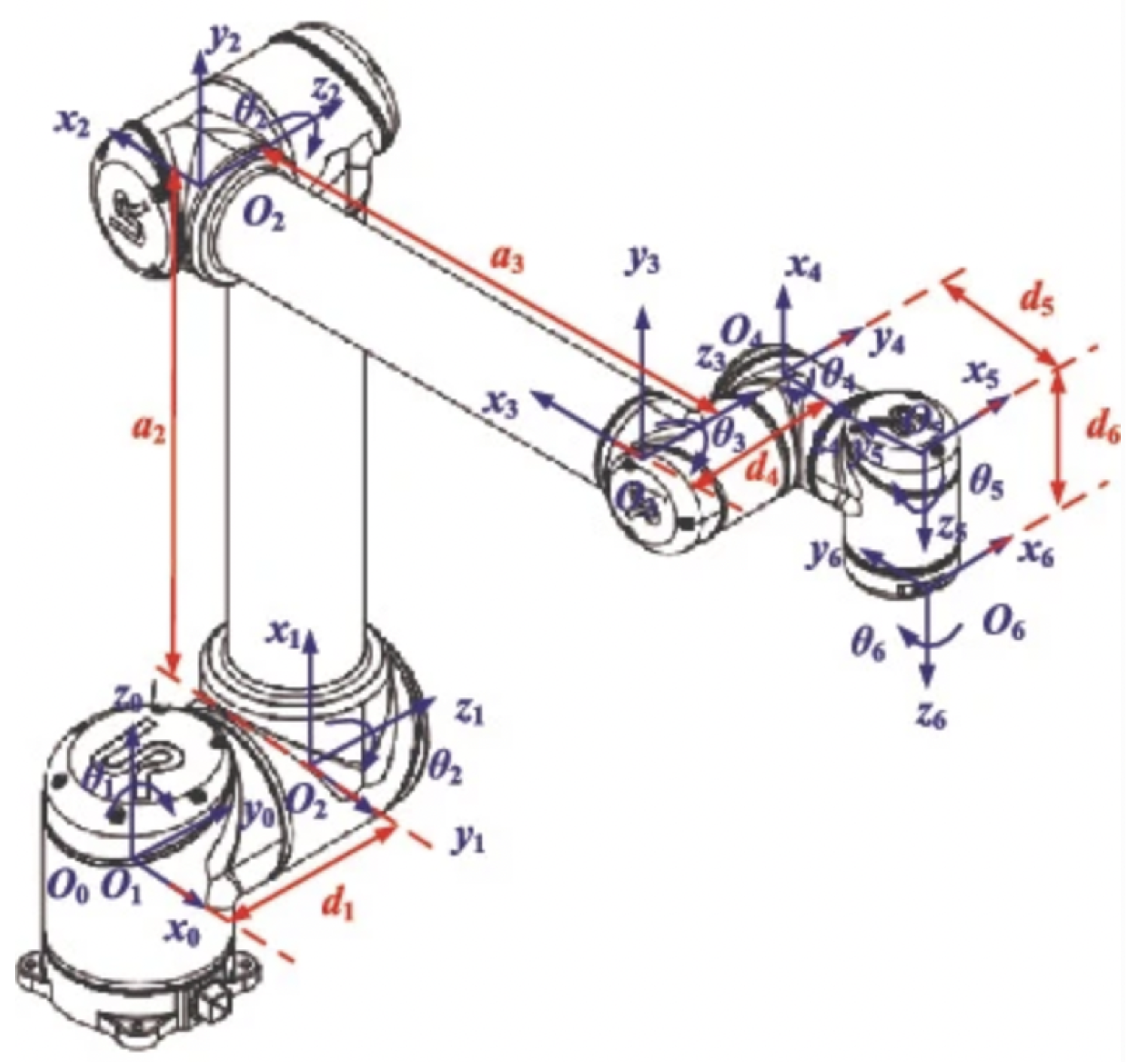
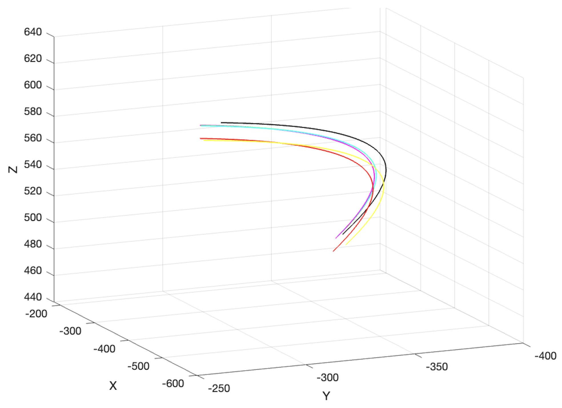
As previously described, the database is obtained by sampling and feature extraction of the trajectories of the robotic arm, the algorithm of forward kinematics of manipulator is given in Appendix A. As shown in Figure 5, the trajectories of the six joints of robotic arms of UR10 are sequentially injected with a 1-degree fault, and it can be seen that some of them overlap extremely well.

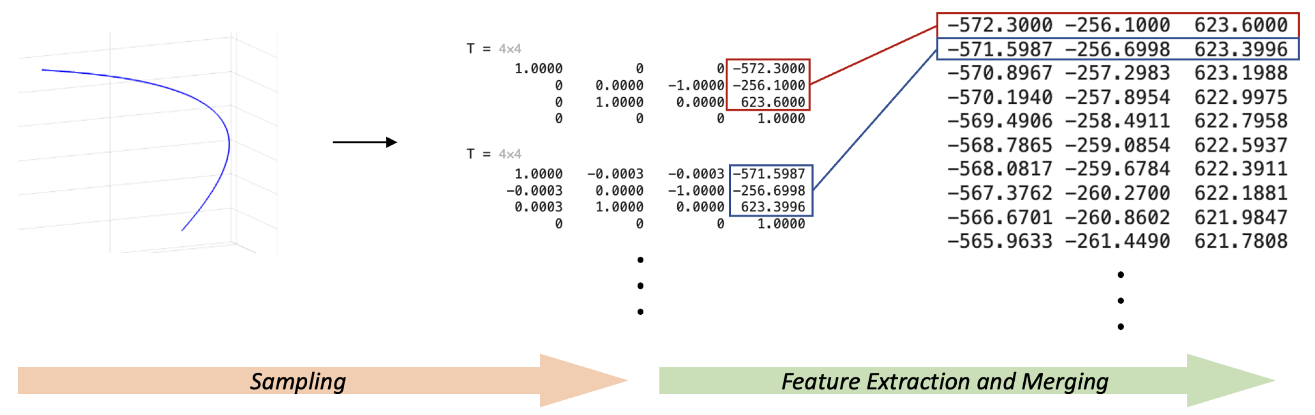
There are seven trajectories in total, one of which is the trajectory without fault. The data obtained from each sampling is a 4 × 4 matrix from the base to the actuator and, if the positions of each trajectory at each sampling are needed, they need to be extracted in the following way (Figure 6).

The total number of databases is the product of the number of samples and the trajectory, and each as a location single feature data currently consists of three numbers. At the same time, if the goal is to separate the different faults using a neural network, the characteristics of the robotic arm itself need to be taken into consideration, and the trajectory can only reflect one feature, the end-effector positions.

3.3. BP Neural Network for Classification

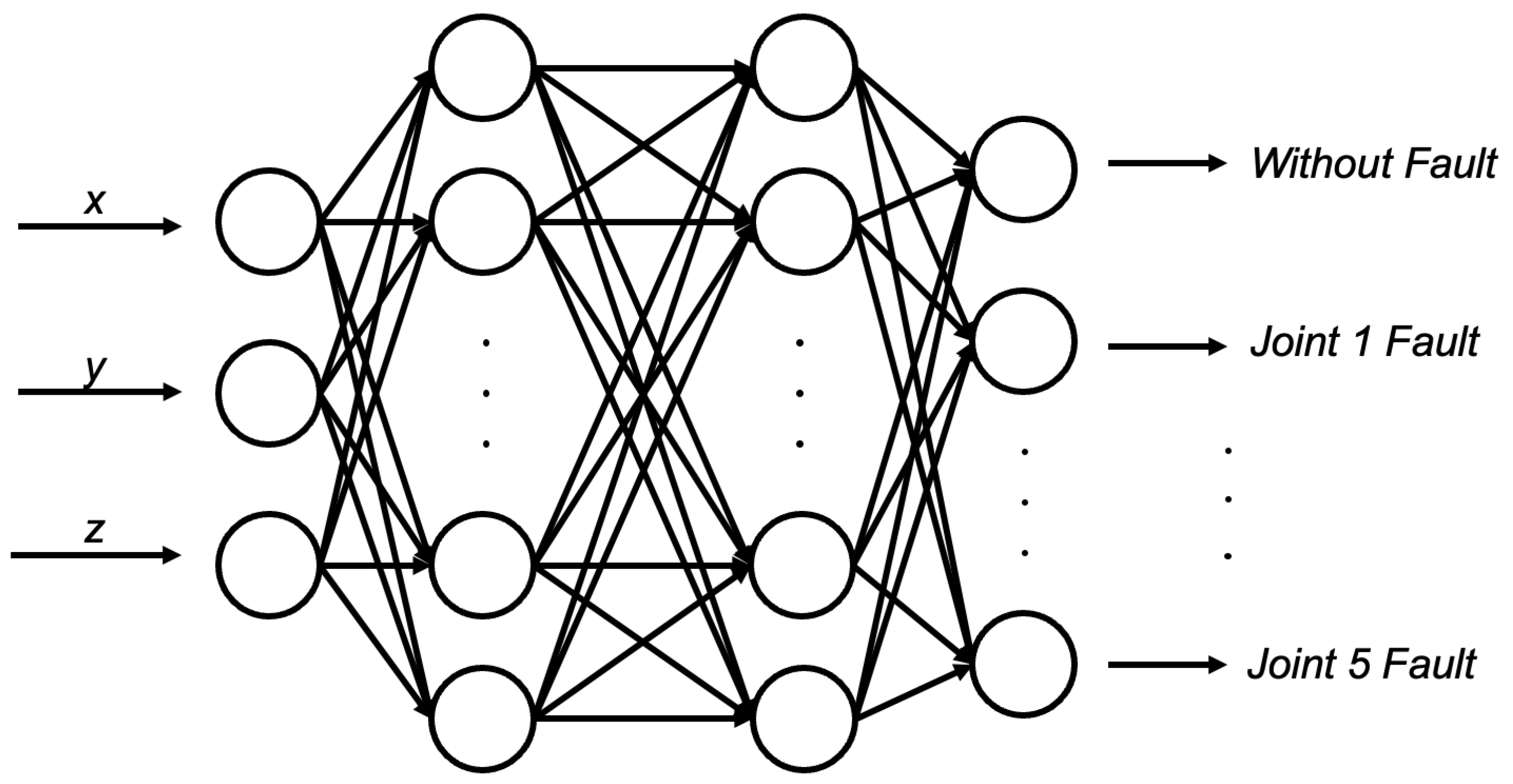
The task of the neural network here is to act as a classifier to classify the trajectories in Figure 5. Since the trajectories of the sixth joint of the robotic arm are characteristic of a fault, and no faults are the same and therefore cannot be classified, the first step is to consider only the six trajectories generated by the no fault condition and the first five joints fault in sequence to classify them, so as to achieve the preliminary fault diagnosis. The feature extraction of the position of the actuator at the end of the robotic arm is mentioned above, and combined into one data set; the structure of the network is shown in Figure 7. There are three inputs and six outputs, which include two hidden layers of the neural network and the inputs of the neural network from the x y z positions of the database, and the outputs are six classifications. In addition to this, a label matrix needs to be pre-designed, i.e., for an experiment with n samples per trajectory, the label matrix is 6n × 1, and the labels are changed every n rows to achieve that each trajectory has its own corresponding label for classification.

In order to obtain information about the effect of different sampling numbers, i.e., database sizes, on the results, the number of samples per trajectory was set to 1500, 5000, and 10,000, respectively, when the fault injection was one degree, and the total database size was the number of samples of a single trajectory multiplied by the number of trajectories (6). In total, 70% of the data will be used as a training set, and 15% of the remaining data will be used as a validation set and a test set, respectively. The results of the network structure, related parameters and training are shown in the following tables, where the

Table 1. Network training results of joint diagnosis for robots. Size of joint angle error = 1° (single feature: position).

Sampling Number	Number of Epochs	Layers	Accuracy (%)	Cross-Entropy Loss
1500	400	3-11-11-6	94.33	0.2318
5000	400	3-11-11-6	96.33	0.2152
10,000	400	3-11-11-6	96.80	0.1125

,

Table 2. Network training results of joint diagnosis for robots. Size of joint angle error = 0.5° (single feature: position).

Sampling Number	Number of Epochs	Layers	Accuracy (%)	Cross-Entropy Loss
1500	800	3-11-11-6	89.83	0.2762
5000	800	3-11-11-6	93.10	0.3324
10,000	800	3-11-11-6	95.97	0.2872

and

Table 3. Network training results of joint diagnosis for robots. Size of joint angle error = 0.2° (single feature: position).

Sampling Number	Number of Epochs	Layers	Accuracy (%)	Cross-Entropy Loss
1500	800	3-11-11-6	83.24	0.5131
5000	1200	3-11-11-6	87.02	0.4283
10,000	1200	3-11-11-6	91.31	0.4096

show the result of network training with different size of injected fault. It can be seen that the fault diagnosis accuracy of the neural network reaches more than 94% when the fault injection is one degree, and improves with an increase in data.

This means that, when classifying a section of trajectory, a relatively accurate diagnosis of the trajectory with or without fault, and which specific joints are in fault, can be determined. If the goal is to diagnose faults more accurately, a good way is to reduce the size of the injected faults by setting the size of the injected faults to 0.5 and 0.2 degrees and repeating the above steps, the results of which are shown in

Table 4. Network training results of joint diagnosis for robots. Size of joint angle error = 1° (single feature: attitude).

Sampling Number	Number of Epochs	Layers	Accuracy (%)	Cross-Entropy Loss
500	800	3-13-13-7	64.00	0.8464
1500	800	3-13-13-7	65.48	0.7317
5000	800	3-13-13-7	64.53	0.7383

and

Table 5. Network training results of joint diagnosis for robots. Size of joint angle error = 1° (dual features).

Sampling Number	Number of Epochs	Layers	Accuracy (%)	Cross-Entropy Loss
500	400	6-13-13-7	97.67	0.4082
1000	350	6-13-13-7	99.48	0.3265
1500	350	6-13-13-7	99.62	0.1708

.

It can be seen that, if the size of the injected faults is reduced to achieve an increase in diagnostic accuracy, the accuracy of the classification of the corresponding neural network will be reduced and the number of epochs required will increase, which means that more time and resources are required for fault diagnosis and there is a high risk of overfitting. Analysing the above study, the following conclusions can be drawn: firstly, the diagnostic correctness is higher when the injected fault size is one degree, and the accuracy decreases but is still acceptable when the fault size is small. Secondly, classifying the positions of the end-effector as features can only achieve fault diagnosis for five joints, and the overall required data set is relatively large, requiring 60,000 sets of data and 1200 epochs to achieve an accuracy of 91% when the fault is 0.2 degrees, which is unrealistic in practical applications. When analysing the reasons for the lack of accuracy of the classifier, it is believed that the data, i.e., the positions of the end-effector, are not good enough to classify the existing trajectories and, even if there are only six segments of trajectories, there is also the problem that each segment of the trajectory has a strong correlation with the others, e.g., if the injected fault is 0.2 degrees, which is shown in Figure 8, the six segments of trajectories overlap more than in Figure 5, which has a 1-degree fault of the joint, and it is difficult to differentiate them even by the naked eye.

When analysing the tasks of the individual joints of the robotic arm, Section 2 states that the sixth joint is used to control the rotation of the robot’s wrist around its own axis, i.e., the rotation of the robot’s end-effector. This means that it is possible to distinguish between faulty and fault-free trajectories of the sixth joint characterised by the orientation of the end-effector with respect to the base. Therefore, the attitude of the end-effector is used as a feature to achieve trajectory classification and fault diagnosis; the attitude is represented by the Pitch, Roll and Yaw in the Euler angles; the three values corresponding to the attitude feature are also extracted from its sub-transformation matrix in the robotic arm DH; the process of the feature extraction has already been given above; the rest of the algorithms are the same; and there are seven neurons in the output layer of the neural network (because the attitude can be put into the sixth joint faults from fault-free trajectories). It was found that the classification accuracy of the seven labelled data were found to be only about 65% when the injected fault was one degree, and the accuracy was independent of the database size for the same number of epochs. The results are shown in

Table 6. Network training results of joint diagnosis for robots. Size of joint angle error = 0.5° (dual features).

Sampling Number	Number of Epochs	Layers	Accuracy (%)	Cross-Entropy Loss
500	800	6-13-13-7	94.33	0.4544
1000	700	6-13-13-7	97.29	0.3926
1500	600	6-13-13-7	99.76	0.3751

.

The reason for this result is that, compared to using actuator positions as features, the actuator attitudes in each segment of the trajectory after injecting faults into each joint are more highly correlated with each other, and are more difficult to be extracted by the neural network. For example, the third and fourth joints have the same attitude of the end actuator after fault injection, the sixth joint has exactly the same Roll value as without fault, etc. This high correlation between differently labelled database at single-feature three data can greatly affect the classification accuracy of the neural network. Therefore, in summary, it was decided to use multi-feature fusion for fault diagnosis.

3.4. Multi-Feature Fusion for Optimal Fault Diagnosis

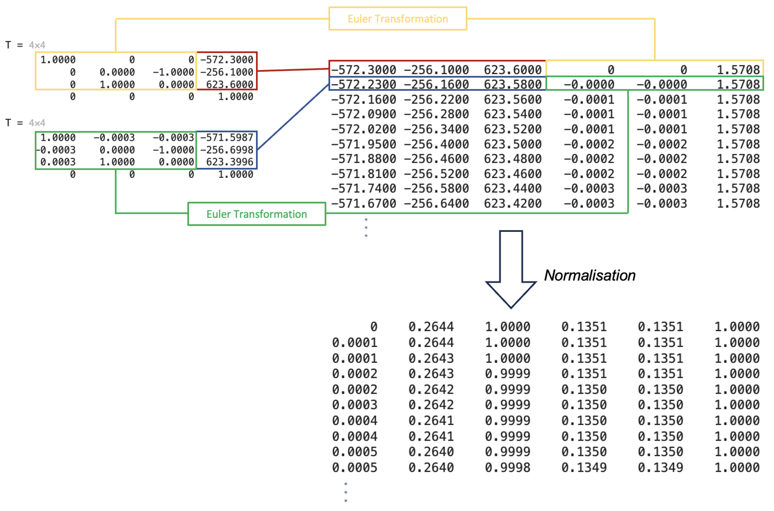
According to the research and analysis above, it can be found that the influence of each joint on the positions and attitude of the actuator is complex, and can be transformed into a 1 × 3 matrix form after the extraction of both features. Due to the different magnitude of the position and Euler angle values, they need to be normalised before feature fusion. The study above, when using actuator positions and orientation as features, respectively, reveals that the positional features have a greater impact on classification accuracy, although their number of classifications is one class less than the number of orientations as a single feature. Finding the weights of single features in multi-feature data for their influence on classification effectiveness is a popular and complex topic, and commonly used methods include grid search, genetic algorithms, etc., but none of them are applicable in this paper due to the large amount of resources and time they require. Considering that the feature of neural network algorithms is to constantly update the weights on the synapses by gradient descent method to achieve better accuracy, the simplest feature concatenation is adopted, i.e., two 1 × 3 features are spliced side by side (concatenation) to form 1 × 6 data, which are shown in Figure 9, and the most suitable weights are found through the training of the network. The following figure illustrates the extraction, concatenation and normalisation of the two-feature data.

For the new database containing two features, the input layer of the neural network consists of six neurons corresponding to the position x y z and direction pitch roll yaw information, and the output layer contains seven neurons corresponding to the seven trajectory classifications in the six joints in faulty and fault-free states, with no change in the generation of the labelling matrices. The classification results of the neural network trained with the dual-feature database are shown in

Table 7. Network training results of joint diagnosis for robots. Size of joint angle error = 0.1° (dual features).

Sampling Number	Number of Epochs	Layers	Accuracy (%)	Cross-Entropy Loss
500	1000	6-13-13-7	89.21	0.7011
1000	800	6-13-13-7	93.92	0.6425
1500	800	6-13-13-7	95.99	0.6312

, and it can be noticed that the number of database used is much less compared to the previous single-feature, only 3500 sets of data can achieve more than 97.50% classification accuracy when the injected faults are one degree, and there is a 99.81% accuracy when the number of single-trajectory samples is 1500, which is the same as that of single-position position features with one additional feature. This is an improvement of five percentage points compared to the unit-placement position feature with one more classification.

Repeating the previous procedure to shorten the size of the injected fault, the corresponding classification accuracy and single-feature classification improved with a reduced database and an increased number of classifications, and the diagnosis of 0.1 degree joint faults was achieved; the results are shown in

Table 8. Network training results of joint diagnosis for robots. Size of joint angle error = 0.1° (three features).

Sampling Number	Number of Epochs	Layers	Accuracy (%)	Cross-Entropy Loss
300	500	9-13-13-7	91.21	0.8119
600	400	9-13-13-7	95.92	0.7325
1000	400	9-13-13-7	96.72	0.6964

and

Table 9. Overview of neural network training results for different configurations of features.

Configuration of Features	Size of Database	Size of Fault (${}^{\circ }$)	Accuracy (%)
Single Position	70,000 × 3	0.5	95.97
Single Attitude	35,000 × 3	1.0	64.53
Position and Attitude	7000 × 6	0.5	97.29
Position, Attitude and Acceleration	4200 × 9	0.5	98.34

. The diagnostic accuracy of the classifier can be more than 99% when the fault is 0.5 degrees, and can be close to 96% at 0.1 degrees; this result is much more accurate compared to any single feature.

It can be clearly seen that the database created by the dual features of position and attitude of the actuator makes the neural network much more capable of classification, and the main advantage over the single feature classification is the increase in accuracy, the smaller database required, and the greater precision. Inspired by the dual feature and [19], the acceleration of the end-effector in the three directions, xyz, is added as the third feature. From the perspective of the robotic arm, it is assumed that the change in the actuator orientation and position predestines the acceleration of the actuator in the xyz directions to be different as well, which again increases the characteristics of each labelled data, which makes the neural network better for classification. The acceleration can be obtained from the second-order derivative of the three-direction xyz position change between each sample, then transformed into a 1 × 3 matrix, and the position and direction features are spliced and fused, so that each set of data is a 1 × 9 matrix, and the number of neurons in the input layer is nine. Each set of data consists of nine numbers containing the three features of the actuator. The classification ability for neural network of the database built by three features is shown in Figure 10.

When the injection fault is 0.1 degrees, it can be seen that compared with the two-feature database, the neural network requires a smaller database and the accuracy is also improved. When injected fault is 0.5 or 1 degree, the accuracy is also better. But the overall accuracy remains at about the same order of magnitude, and there is no particularly significant change, indicating that the acceleration features to a certain extent can differentiate between the different trajectories, but the ability to differentiate is limited. It can be noticed that, in the case of multiple features, although the accuracy is improved, the corresponding cross-entropy loss is also more than before. The possible reason for this is that the model is very confident in all the predictions, i.e., the probability of prediction is very close to 1 for the correct category and very close to 0 for the other categories. Then, even if the predictions are mostly correct, a single incorrect prediction may lead to a very high cross-entropy loss. To fully evaluate the performance of a neural network as a classifier, it is not sufficient to rely only on accuracy and cross-entropy loss, only an initial judgement is made here. The performance of the network will be further evaluated in the next section, in conjunction with other metrics.

4. Computational Experiments

A Matlab simulation is used to conduct the whole computational experiment, which bench tests the framework configuration, procedure functionality, algorithm efficiency, and numerical accuracy in detection/diagnosis of various of faults.

4.1. Experimental Evaluation of Single Size of Fault

Because of the different tasks of each joint of the robotic arm, the neural network has different classification effects for databases built with different features, which means different fault diagnosis precision and accuracy, as shown in the table below (Table 9).

As can be seen from the table, when meeting the requirement of a 95% accuracy rate under other conditions being the same, the three-feature fusion establishes the smallest data size, and only needs to sample each segment of the trajectory 600 times to obtain an accuracy rate of 98.34%. And, although the neural network classification corresponding to the two-feature data is not as effective as that of the three-feature data, the accuracy also reaches 97.29%, which meets the previously proposed requirement of more than 95%. At the same time, the arithmetic power required to calculate the acceleration is larger, and it is necessary to find the derivatives of the rate of change of the neighbouring samples of each segment in the three directions, which is the second-order derivative, and this will increase the load of calculation considerably.

So, the classification effect of the corresponding neural network with dual features will be evaluated. As an example, in the experiment corresponding to Table 7, when the number of samples is 1500, the group of experiments achieved a very high accuracy of 99.62%, but at the same time, the cross-entropy loss is also 0.1708, which can be noticed that the cross-entropy loss of each group of experiments is on the high side compared to the accuracy, and the network will be continuously evaluated below in conjunction with metrics such as the ROC curves and the confusion matrices, which is shown in Figure 10 and Figure 11.

Figure 10. Confusion matrix of classifier by injected fault at one degree with two features.

Figure 10. Confusion matrix of classifier by injected fault at one degree with two features.

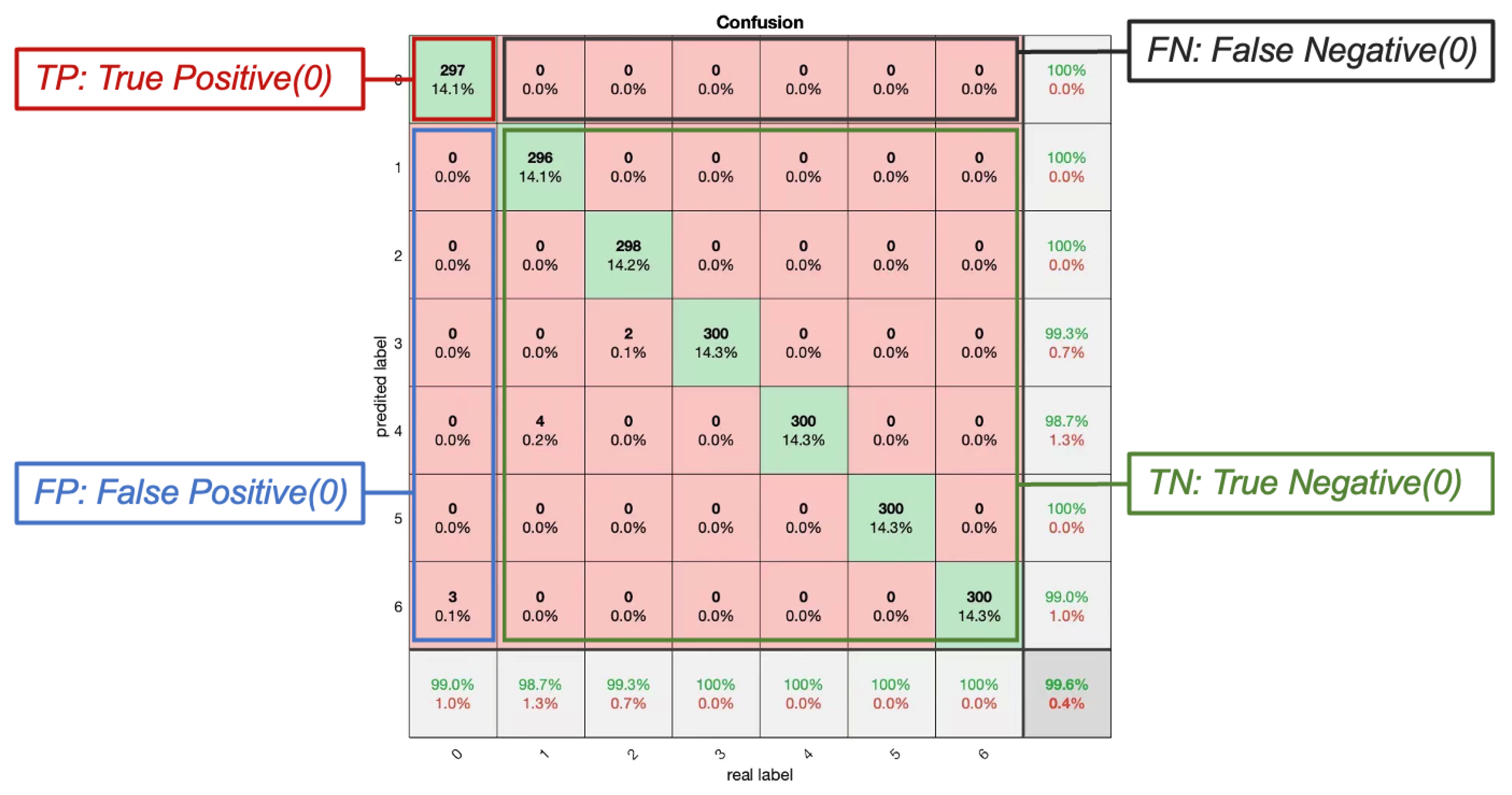
The confusion matrix is usually presented for the results of a test set, to give an idea of how the model actually performs on unseen data. It shows the relationship between the individual categories predicted by the model and the actual categories, and the confusion matrix provides a clear view of how accurately the model predicts each category and when it misclassifies one category as another. When the number of samples per trajectory (category) is 1500, the corresponding 20% as a training set is 300. The 99.6% in the bottom right corner indicates the classification accuracy of the neural network, which means that there is a 99% probability that each classification is correct.

The horizontal and vertical axes of the confusion matrix are the true and predicted labels, respectively. For data with label 0 (no faulty trajectory), the red box in the upper left corner indicates that the actual value is the same as the predicted value, i.e., true positive (TP), which is 297. The blue box on the left side indicates that the actual value is positive (False Positive, FP); in our example, three data with label 0 are predicted to have label 6, and the TN value is the sum of the values in the corresponding columns, except for the TP value, which is 3. The black box is false negative (FN), which indicates that the actual value is positive in our example, but the model predicts it to be negative, i.e., some other labelled class. The value of FN, which can be computed from the neighbouring rows except for the TP value, is zero. The green box is True Negative (TN), which indicates that the actual and predicted values have the same meaning, and it is the sum of the values of all non-0 rows and columns, which is 1800. For data labelled as 0, TP, FP, FN and TN can help to implement more metrics specific to that category, such as accuracy for fault-free trajectory diagnosis:

$$\begin{array}{c}\mathrm{Precision}\left(0\right)=\frac{\mathrm{TP}}{\mathrm{TP}+\mathrm{FP}}=\frac{297}{297+3}=99\%\hfill \end{array}$$

(6)

This means that for data labelled 0, there is a 99.85% probability that each classification prediction is correct.

$$\begin{array}{c}\mathrm{Accuracy}\left(0\right)=\frac{\mathrm{TP}+\mathrm{TN}}{\mathrm{TP}+\mathrm{TN}+\mathrm{FP}+\mathrm{FN}}=\frac{297+1800}{297+1800+3+0}=99.85\%\hfill \end{array}$$

(7)

Precision means that if a label is identified as class 0, then there is a 99% probability that it belongs to that class.

$$\begin{array}{c}\mathrm{Recall}\left(0\right)=\frac{\mathrm{TP}}{\mathrm{TP}+\mathrm{FN}}=\frac{297}{297+0}=100\%\hfill \end{array}$$

(8)

Recall means that if a data belongs to class 0, then there is 100% probability of being predicted correctly. With the confusion matrix, some parameters can be calculated for specific individual classifications, calculated in the same way as above, and it can be seen that training the neural network with dual features when the injected faults are one degree and the number of samples of a single trajectory is 1500, which has a very good classification effect.

In addition to the confusion matrix, another commonly used metric for evaluating classifier performance is the ROC curve, which is a reflection of the relationship between sensitivity and specificity. The horizontal position X-axis is the specificity metric, also known as the false positive rate (false alarm rate), and the closer the X-axis is to zero, the higher the accuracy is; the vertical position Y-axis is known as the sensitivity, also known as the true positive rate (sensitivity), and a larger Y-axis represents a better accuracy. According to the position of the curve, the whole graph is divided into two parts. The area of the lower part of the curve is called the Area Under Curve (AUC), which is used to quantify the overall performance of the ROC curve and indicate the prediction accuracy; the higher the AUC value, that is, the larger the area under the curve, the higher the prediction accuracy. The closer the curve is to the upper left corner (the smaller the X, the larger the Y), the higher the prediction accuracy. The test set ROC curve for the neural network model after the above experiment is shown in Figure 11.

Figure 11. ROC curve by one degree injected fault with two features.

Figure 11. ROC curve by one degree injected fault with two features.

As can be seen from Figure 11, the ROC curves for all seven classifications fit perfectly on the upper left axis, and the corresponding AUC values are all one, which means that the model achieves perfect prediction under all thresholds, i.e., the trade-off between the True Positive and False Positive rates is optimal. In other words, the model has a strong ability to distinguish between positive and negative categories well. But, on the other hand, there may be some problems in this case, such as data overfitting, which means that the model may have over-learned the features and noise in the training data, resulting in a very good performance on the training data, but the prediction of the new data may not be as good, i.e., the generalisation error will be larger. Overall, the performance of the neural network model for classification of fixed trajectories is still excellent, and the near-perfect performance also leads to the fact that a single incorrect prediction may also lead to a very high cross-entropy loss, as previously conjectured.

Experiments have proved that neural network-based robotic arm fault diagnosis is a very reliable approach. Firstly, the neural network analyses and diagnoses the possible faults of the robotic arm through the complex pattern recognition ability and adaptive learning ability. In this paper, the neural network handles the data of the two features of the robotic arm position and attitude, on the basis of which velocity, vibration, etc., can also be used as features for multi-feature fusion in future research according to the environment. A major advantage of processing the fused data with neural networks is that the neural network does not require the researcher to weight its features by virtue of its own algorithmic advantages. And, compared to other ways of embedding hardware, neural networks and the proposed embedded applications reduce human intervention and cost.

4.2. Mixed Diagnostics for Multi-Size Faults

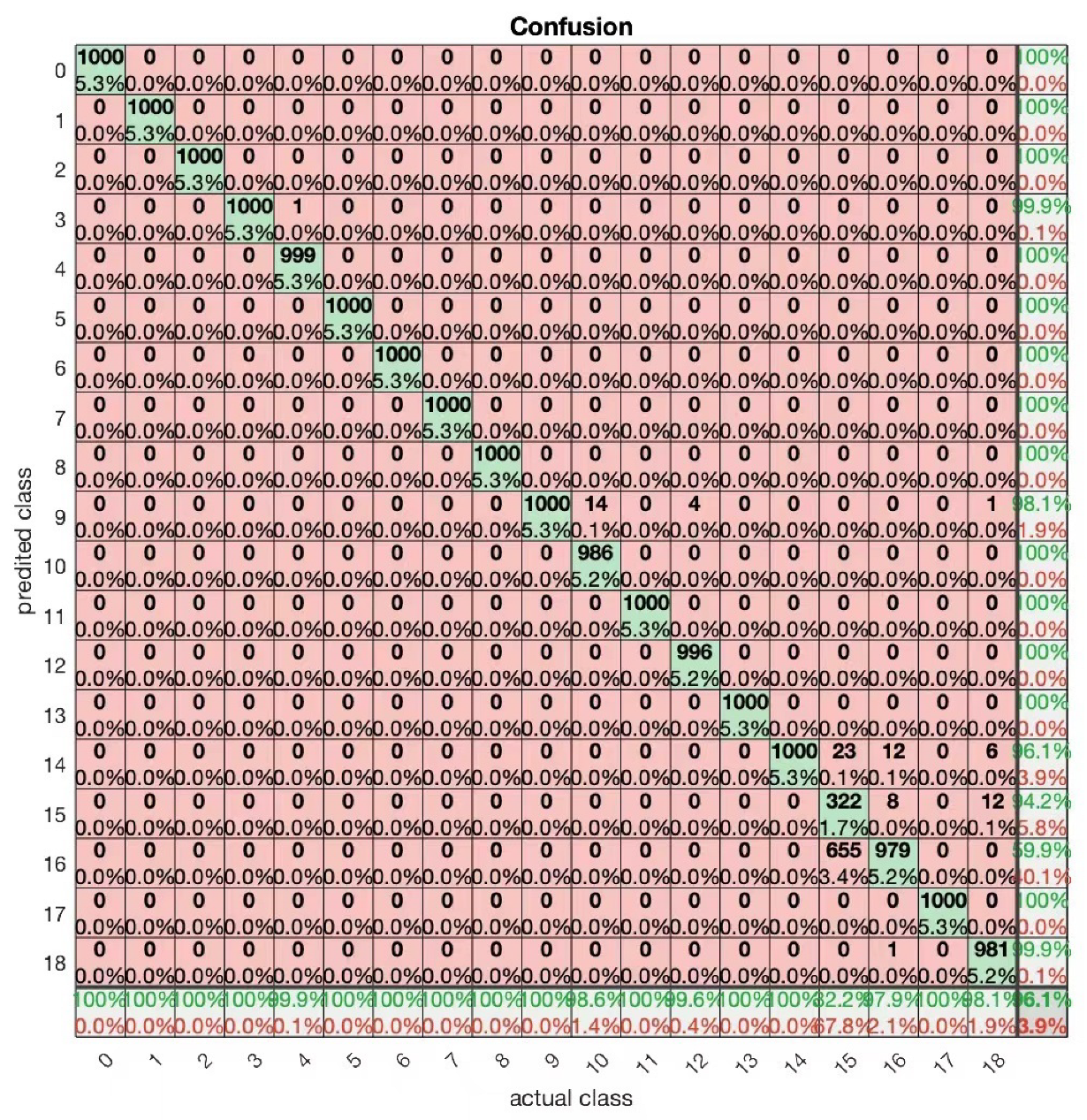
In the practical application of different requirements for the accuracy of the robotic arm task, a single size of the injected faults can not meet the demand if the trajectories generated by different sizes of the injected faults are put into the same network, i.e., in addition to a fault-free trajectory, there are 18 different joints with different fault sizes, and a total of 19 trajectories corresponding to the accuracy of the 19 classifications in the experiments using dual-featured data training network were found. The result is average, and the accuracy is only about 80%, but if the sampling number of a single trajectory is set to 5000, a total of 95,000 sets of data are fed into the network for training, validation and testing, the result is more satisfactory, and the accuracy can reach 96.1%. The structure of the network is basically the same as the above experiments, the only modification is that there are 19 neurons in the output layer. The corresponding confusion matrix is shown in Figure 12.

It can be seen that for most of the trajectories, the neural network is able to classify them well, this classification means that it can be precise as to which joints have what fault error, it is worth noting that the fifteenth classification has a lower accuracy rate, calculated as per the above methodology is only 21%, and the precision rate is only 33%, as can be seen from the data, for every 1000 sets of data corresponding to a label of 15 there are 322 were able to be correctly classified, with a large proportion predicted to be labelled 16. this means that a large proportion of third joint faults are classified as fourth joint faults when the injected fault is 0.1 degrees. A possible reason for this is that the third and fourth joint faults correspond to the same actuator orientation, since the third joint only controls the extension and retraction of the robot arm, and there is very little difference in the position of the actuators at an error of 0.1 degrees; In other words, the two trajectories are highly coincident. The neural network is able to distinguish and classify these two well even for 0.1 degree faults during the previous single-size injection faults. A possible reason for this is that with so many classification labels, it is difficult for the network to find the difference between the two labels so it is also difficult to distinguish these two labels accurately. 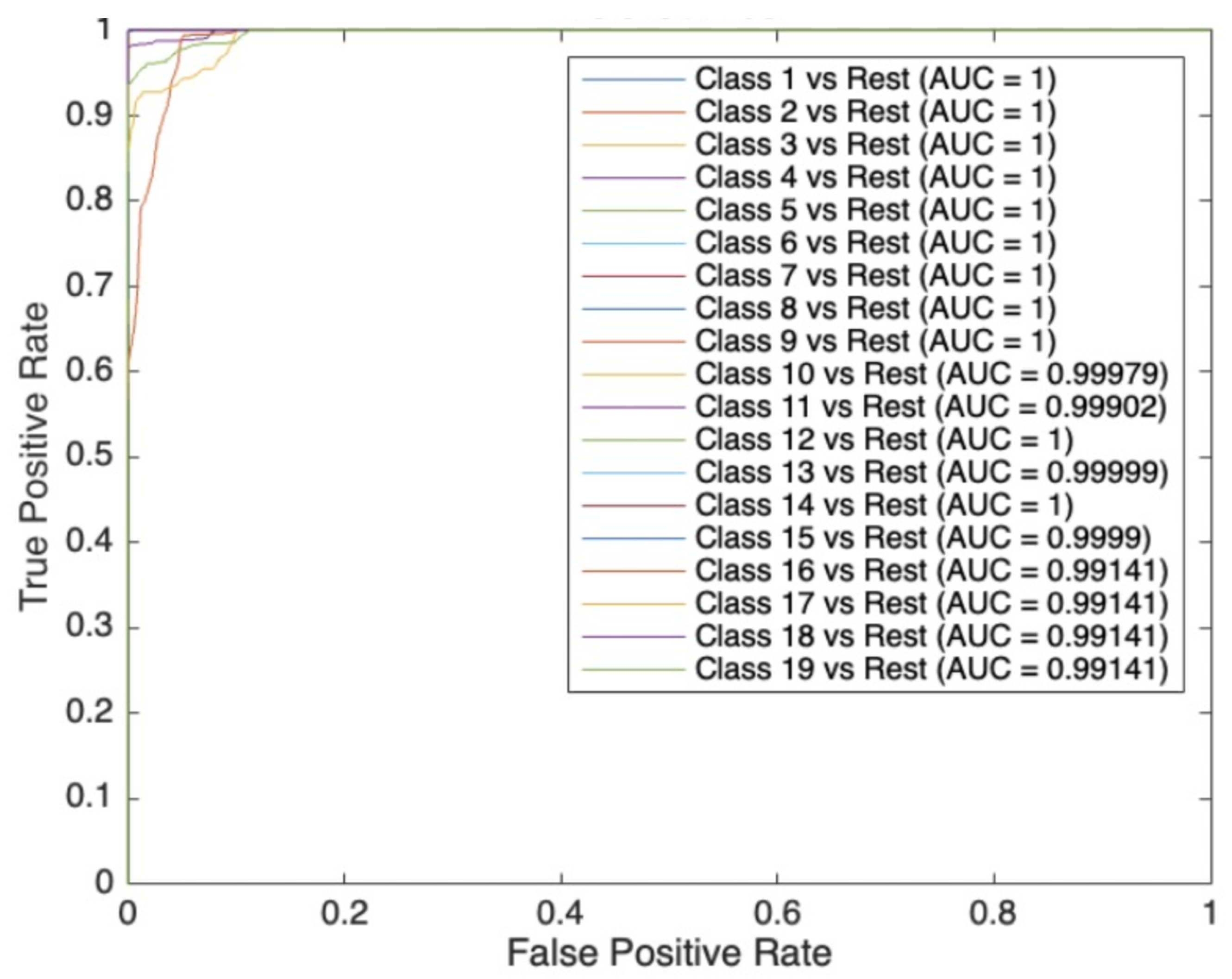The performance of the neural network in classifying the 19 labels can be evaluated more comprehensively with the help of ROC curves, the corresponding ROC curves are shown in Figure 13.

The percentages in the bottom row of the figure can be used to measure the performance of the model on negative categories, such as the false alarm rate, which is non-zero in columns 5,10,12,15,16, and 18 of the row, which are 0.1%, 1.4%, 0.4%, 67.8%, 2.1%, and 1.9%, respectively, e.g., the 0.1% in the fifth column indicates that for the data corresponding to the label (4) there is a 0.1% probability that the be misclassified.The percentages in this rightmost column can be used to measure the performance of the model on positive classes, such as Recall, which is 99.9%, 98.1%, 96.1%, 94.2%, 59.9%, and 99.9% for rows 4, 9, 14, 15, 16, and 18, respectively, meaning that there is a corresponding probability of classifying the data correctly, and that the data in the other rows is 100%, which means that it will do the classification completely correctly.

From the figure, it can be seen that the AUC values of all curves are above 0.99, and most of the classified labels correspond to an AUC of 1, while the labels starting from 14 and onwards have an AUC of less than one, which corresponds to the fault trajectory of each joint when the injected faults are 0.1 degrees. Label 15, on the other hand, corresponds to an AUC of 0.9999, while the accuracy of the predictions made for it is only 21%. The main reason for this is the difference between accuracy and ROC, i.e., accuracy is a threshold-dependent metric, whereas ROC and AUC are independent of the threshold. Therefore, despite the low accuracy, the AUC may still be high, as long as the model is able to discriminate well between positive and negative samples.

Overall, the performance of the BP neural network is acceptable and trustworthy for 19 classifications, which is very important for practical applications and can be used in a wide range of generally applicable applications, depending on the accuracy requirements of the task, which indicates that there is a wider range of applications possible in practical applications. In conjunction with the above research, the use of complex pattern recognition capabilities of neural networks to analyse and diagnose possible malfunctions in robotic arms is very effective and possible in industry: this research not only diagnoses a malfunction in one of the joints of a robotic arm by means of the trajectory of the movement, but also classifies the dimensions of the malfunction with precision. 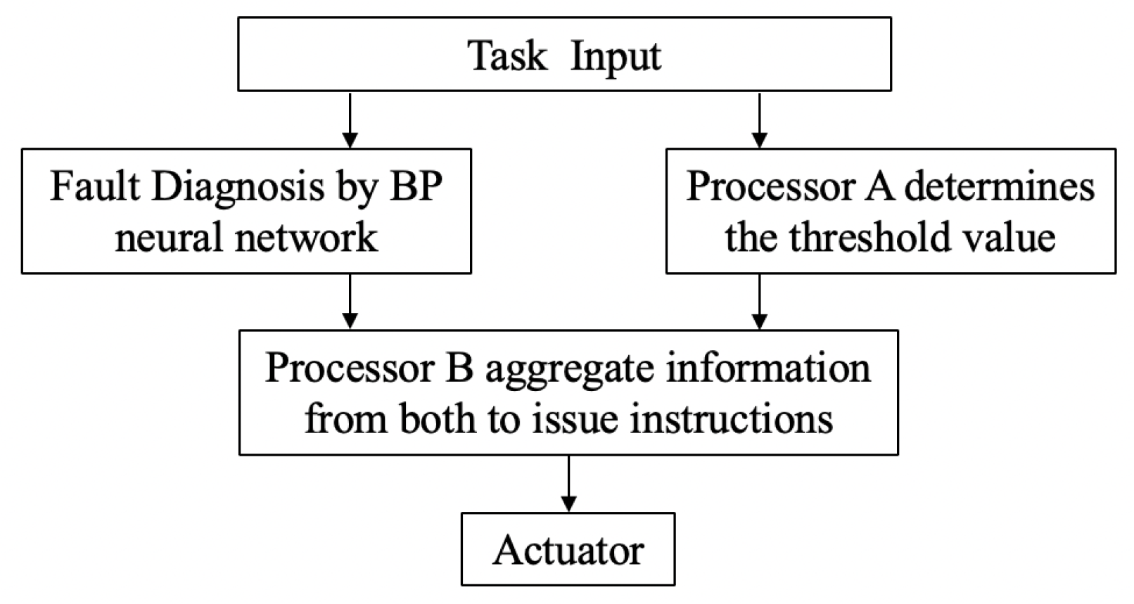It can be applied practically according to the requirements of the task, and Figure 14 shows the possibilities of an embedded application.

Firstly, the engineer inputs the actual task according to the needs of the production line, and then performs a BP neural network based fault diagnosis on the trajectory of the robotic arm. If the predicted classification is 0, indicating no faulty trajectory, then output 0. If the predicted classification for the trajectory of the robotic arm is between 1 and 13, i.e., the error is 0.5 or 1 degree, then output 1. If the output is 14 and above, output 2, which indicates that the fault of a certain joint is 0.1 degree. At the same time, processor A defines the accuracy type according to the actual task and the set task accuracy requirement (the highest accuracy level is 0, the second highest accuracy level is 1, and the lowest accuracy level is 2) and outputs it to processor B. Processor B receives the classification level of the neural network and the level of the task accuracy requirement, and performs the judgement according to the set information, then outputs the signal to the signal lamp (actuator).

5. Conclusions

In this applied demonstration study, UR10 is selected as an exemplary research object, and its end-effector information, including position and attitude, are extracted as features training database for a BP neural network classifier. The developed diagnostic procedure has considered the different fault sizes of different joints, the accuracy, and all other metrics such as the confusion matrix and ROC curves, and the simulated results are in line with the expectations, which meets the requirement of the practical applications and is expandable to the other robot systems in principle [20]. The main contributions of this research are as follows:

• A new experimental design is proposed to extract the required features and create a database through the DH algorithm for the positive kinematics of the robotic arm;
• A new scheme for the diagnosis of robotic arm joint faults has been developed through existing robotic arm algorithms and a neural network algorithm;
• Existing methods have been optimised to detect robotic arm motion and identify faults in real time with a neural network that can be accurate down to the size of fault and joints.

Although the location and accuracy of the faults are relatively high, they cannot be corrected automatically, and the intervention of engineers is needed to investigate the causes of the faults, and judgements of the angular faults can only initially investigate the faults of the robotic arm itself [7]. Overall, neural network-based fault diagnosis research can be further optimised, such as through other features, to further differentiate between the various fault generation trajectories. The smaller size of the fault can be compensated for through control, and the structure of the network can also be better optimised to reduce the generalisation error and thus achieve better applications.

In practical applications, the position and orientation of the robotic arm during movement can be recorded by robotic software such as ros, fed into a trained neural network for classification, and the neural network, an additional plug-in, can be implemented in an embedded way.