Survey of Recent Applications of the Chaotic Lozi Map

Abstract

Since its original publication in 1978, Lozi’s chaotic map has been thoroughly explored and continues to be. Hundreds of publications have analyzed its particular structure and applied its properties in many fields (e.g., improvement of physical devices, electrical components such as memristors, cryptography, optimization, evolutionary algorithms, synchronization, control, secure communications, AI with swarm intelligence, chimeras, solitary states, etc.) through algorithms such as the COLM algorithm (Chaotic Optimization algorithm based on Lozi Map), Particle Swarm Optimization (PSO), and Differential Evolution (DE). In this article, we present a survey based on dozens of articles on the use of this map in algorithms aimed at real applications or applications exploring new directions of dynamical systems such as chimeras and solitary states.

1. Introduction

Among the most popular discrete chaotic attractors (Belykh map, Lorenz map, Hénon map, etc.), Lozi’s chaotic map has been thoroughly explored since its publication in 1978, and continues to be today. Hundreds of publications have analyzed its particular structure and applied its properties in many fields, including cryptography, electronic devices such as memristors, optimization, synchronization, secure communications, AI with swarm intelligence, chimeras, solitary states, and more.

Zeraoulia [1] wrote a collection of results published between 1997 to 2013, including 700 references. However, new results in theory and applications are continually being published in many different journals and books, and I am frequently asked about them. This is why I have decided to gather all the new results on applications of this map in the current survey in order to render them easily accessible. All these results are the responsibility of their original authors, not mine.

In Section 2, we recall the origin of this map, its initial definition and classical chaotic properties in the dissipative case, and its dynamics features, including fixed points, invariant manifolds, basin of attraction, etc. I briefly mention a number of new results on advanced properties concerning other statistical, hyperbolic, ergodic, and topological properties (e.g., bifurcation, symbolic dynamics and the kneading sequence, topological entropy, Hausdorff dimension). The chaotic properties in the conservative case are evoked as well. The most recent definitions of the fractional, variable fractional, and complex fractional Lozi map are described. However, the aim of this study is to highlight the applications of this map, not the theoretical results; thus, the presentation of the latter has been reduced to a minimum in order to keep this article to a reasonable length. Interested readers can refer to [2] for an overview of the generalizations of this map.

In Section 3, the use of the Lozi map in electrical devices, memristors, and computers is developed. Section 4 describes the numerous applications of this map in the domain of optimization. Particle Swarm Optimization (PSO), Differential Evolution (DE), and the Self-Organizing Migrating Algorithm (SOMA) are among of the many new algorithms using the Lozi map as a core function. Non-evolutionnary optimization algorithms are described as well, including the Improved Lozi map-based Chaotic Optimization Algorithm (ILCOA).

Applications in control theory are analyzed in Section 5, while applications in cryptography are addressed in Section 6. The coupling of several copies of this map in networks and their synchronization allows for the existence of new theoretical objects (e.g., chimeras, solitary states, and cellular neural networks), as is shown in Section 7. Finally, miscellaneous applications, such as the use of the Lozi map as a benchmark in several studies in the domains of economics and in education, are considered in Section 8, and a brief conclusion is presented in Section 9.

2. The Lozi Chaotic Map

2.1. Origin

On 15 June 1977, 46 years ago, I discovered this piecewise linear chaotic map of the plane. I remember that the idea came to me around 11 am during the defense of the Ph.D. thesis of one of my colleagues in the department of mathematics of the University of Nice (France) [1] (p. xxv).

A week before, I had attended the International Conference on Mathematical Problems in Theoretical Physics in Roma. During the inaugural talk on 6 June, David Ruelle conjectured that, for the Hénon chaotic map, the theoretical entropy should be equal to the characteristic exponent [3]. As explained in [4], this is how I learned of the first example of a chaotic and strange attractor in the plane: the Hénon attractor (see Figure 1). Surprisingly, I had never before met Michel Hénon, who worked a few kilometers from the math department of the university at the Nice Observatory.

Hénon used an IBM-7040 computer to numerically simulate the Lorenz map [5]. He found it difficult to highlight its inner nature due to the very high dissipativity of this map, for which the rate of volume contraction is provided by the Lie derivative of the Lorenz equations. Solving such equations for the parameters chosen by Lorenz provides $V\left(t\right)=V\left(0\right)e^{\frac{-41}{3}}$. Hence, volumes are reduced by a factor ${10}^6$ after one time unit. Hénon, who was a specialist in the motion of planets, had good experience with Poincaré’s map, which inspired him the way to build the metaphoric model in [6]:

$$\left\{\begin{array}{c}{x}_{n+1}=1-a{x}_n^2+y_n,\hfill \\ y_{n+1}=b{x}_n.\hfill \end{array}\right.$$

(1)

This model can be represented by the iterates of any initial point ${\left(x_0,y_0\right)}^T$ belonging to the basin of attraction using the map ${\mathcal{H}}_{a,b}:{\mathbb{R}}^2⟶{\mathbb{R}}^2$

$${\mathcal{H}}_{a,b}\left(\begin{array}{c}x\hfill \\ y\hfill \end{array}\right)=\left(\begin{array}{c}1-a{x}^2+y,\hfill \\ bx.\hfill \end{array}\right).$$

(2)

The contracting properties of this map are only determined by the parameter b. When $b=0.3$, the contraction in one iteration is mild enough that the sheaves of the attractors are distinguishable on a graphic. Finally, Hénon observed the astonishing fractal structure of the attractor on the image drawn by the computer, which amazed the research community.

At that time, I was a young researcher trying to understand bifurcation theory in the field of numerical analysis [7]. This area was not very well known in France. I was working on the discretization of nonlinear problems using the finite element method, in which nonlinear functions are approximated by piecewise linear functions.

During the Roma conference, I tried without success to apply the spirit of the method of finite elements to the Hénon attractor. Back in Nice after this conference, I eventually decided, using paper and pencil, to change the square function of the Hénon attractor, which is U shaped, into the absolute value function, which has a V shape, implying a folding property (the folding property is important for horseshoes, a main ingredient of chaos, as highlighted by Stephen Smale [8]).

I was owner of a small desktop computer (an HP 9820) linked to an HP 9862 plotter. Immediately after the defense I tested this change of function and found a similar attractor of the Hénon attractor, with straight lines instead of curves for the map [9] (see Figure 2).

$${\mathcal{L}}_{a,b}\left(\begin{array}{c}x\hfill \\ y\hfill \end{array}\right)=\left(\begin{array}{c}1-a\left|x\right|+y,\hfill \\ bx.\hfill \end{array}\right)$$

(3)

2.2. Classic Chaotic Properties of the Dissipative Map (|b| < 1)

The Lozi map is called “dissipative” when $\left|b\right|<1$, which means that the image of any subset $\Delta$ by f has a measure which is less than the measure of $\Delta$: $measure\left(f\right(\Delta \left)\right)<measure(\Delta )$.

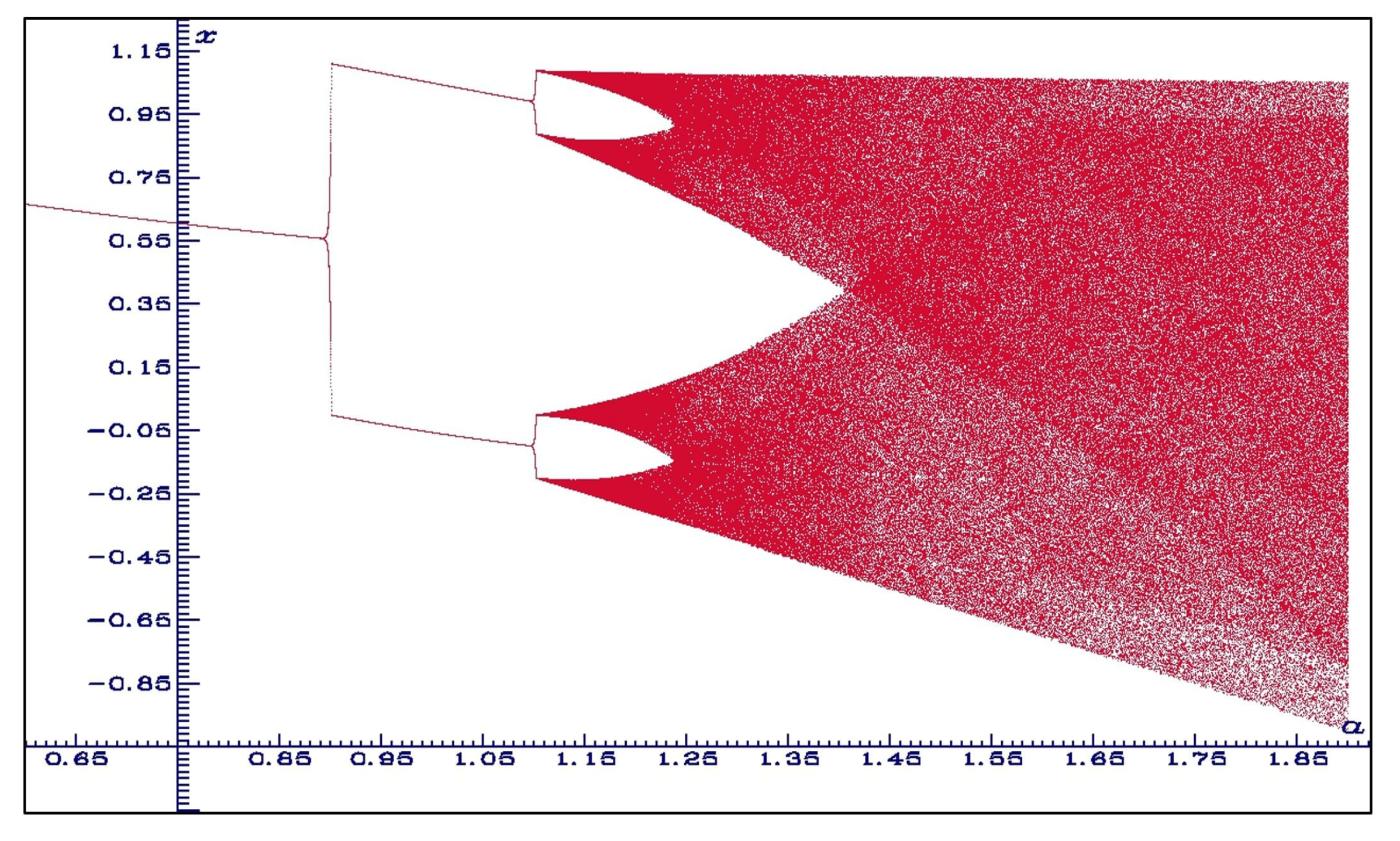
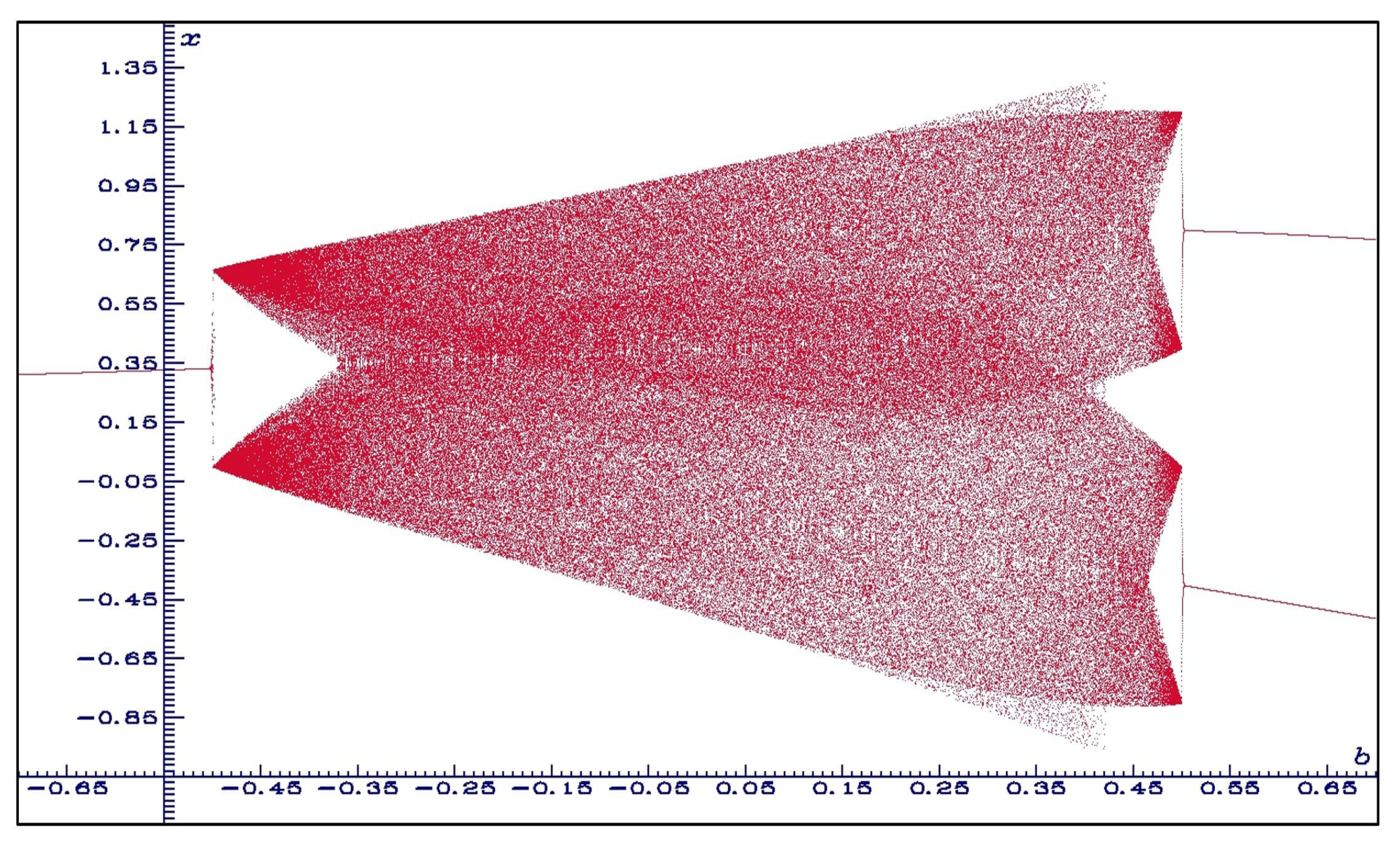
2.2.1. Domain of Existence of Strange Attractor

In 1979, during the International Conference on Nonlinear Dynamics, patronized by the New York Academy of Sciences from 17–21 December, Michal Misiurewicz, in a plenary talk, presented a rigorous proof that for a set of parameters $\mathcal{M}$ this map has a strange attractor, coining on this occasion the name “Lozi map” [10]. This happened only two years after my discovery of this new chaotic attractor, and only one year after its publication [9]. This set in the plane of parameters $(a,b)$ is defined by

$$\mathcal{M}=\left\{(a,b)\left|b>0,a\sqrt{2}<b+2,b<\frac{a^2-1}{2a+1},2a+b<4\right.\right\}$$

(4)

(see Figure 3).

Later, Misiurewicz and Stimac [11] slightly enlarged this set of parameter $\mathcal{M}$ (defined only for $b>0$, and as ${\mathcal{M}}^{+}$ in Figure 4) in the upper edge of the triangle by removing the condition $b<\frac{a^2-1}{2a+1}$.

$${\mathcal{M}}^{+}=\left\{(a,b)\left|b>0,a\sqrt{2}<b+2,2a+b<4\right.\right\}$$

(5)

The case $b<0$ was studied by Cao and Liu [12], and recently by Kucharski [13], who found a quasi-symmetric set of parameters ${\mathcal{M}}^{-}$ (Figure 4). However, the right-hand boundary of ${\mathcal{M}}^{-}$ is not completely symmetric to the right-hand boundary of ${\mathcal{M}}^{+}$.

$${\mathcal{M}}^{-}=\left\{(a,b)\left|-1<b<0,a\sqrt{2}>b+2,b>\frac{-8a+3a^2+\sqrt{-16a^3+9a^4}}{8}\right.\right\}$$

(6)

2.2.2. Fixed Points, Invariant Manifolds, and Basin of Attraction

It is straightforward to explicitly compute the fixed points and periodic orbits of any order of ${\mathcal{L}}_{a,b}$ (3) due to the piecewise linearity of the absolute value.

When $1-a<b<a+1$ (for $a>0$, the regions ${\mathcal{M}}^{-}$ and ${\mathcal{M}}^{+}$ are both in the cone defined by theses inequalities), there exist two fixed points:

$${\mathcal{P}}^{+}=\left(\frac{1}{a+1-b},\frac{b}{a+1-b}\right),{\mathcal{P}}^{-}=\left(\frac{1}{1-a-b},\frac{b}{1-a-b}\right).$$

${\mathcal{P}}^{+}$ belongs to the quadrant $\left\{x\ge 0,y\ge 0\right\}$ and ${\mathcal{P}}^{-}$ to the quadrant $\left\{x<0,y<0\right\}$.

For $a>\left|b\right|+1$, that is, in the domain of the parameter space where both ${\mathcal{P}}^{+}$ and ${\mathcal{P}}^{-}$ coexist, it is easy to compute the local stability of these points by evaluating the corresponding eigenvalues of the Jacobian matrix of ${\mathcal{L}}_{a,b}$. It can be shown that both points are saddles.

Moreoever, Misiurewicz [10] showed that the chaotic attractor of this map belongs to the unstable invariant manifold of ${\mathcal{P}}^{+}$. More exactly, the chaotic (and strange) attractor $\tilde{\mathcal{S}}$ can be constructed from the successive forward iterations of a trapping triangular region T,

$$\tilde{\mathcal{S}}=\bigcap _{n=0}^{\infty }{\mathcal{L}}^n\left(T\right),$$

with T being the triangle with vertices at the points I, $\mathcal{L}\left(I\right)$, and ${\mathcal{L}}^2\left(I\right)$, where I is the point given by the intersection of the unstable manifold of the fixed point ${\mathcal{P}}^{+}$ with the horizontal axis

$$I=\left(\frac{2+a+\sqrt{a^2+4b}}{2(1+a-b)},0\right).$$

The basin of attraction of the attractor is modeled by parts of the stable manifold of the fixed point ${\mathcal{P}}^{-}$, as shown by Baptista et al. [14]. They considered the point X intersection of this stable manifold with the vertical axis. Straightforward computation provides

$$X=\left(0,\frac{b(2-a+\sqrt{a^2+4b}}{(a-\sqrt{a^2+4b})(a+b-1)}\right).$$

They considered certain point U belonging on the horizontal axis as well, first defined by Ishii [15], for which the expression is

$$U=\left(\frac{b(2-a+\sqrt{a^2+4b}(a(1+b)+(1-b)\sqrt{a^2+4b})}{(1-a-b)(a-\sqrt{a^2+4b})(a-\sqrt{a^2+4b})(2b(b-1)+a^2(1+2b)+a(1-2b)\sqrt{a^2+4b})},0\right).$$

Baptista et al. showed that the basin of attraction is bounded by a polygonal line entirely characterized by the points U and X along with their successive preimages.

2.3. Advanced Dynamical Properties of the Dissipative Map (|b| < 1)

An open region $\mathcal{B}$ in the parameter space for which the Lozi map exhibits periodic points of least period n was rigorously determined for all $n>13$ by Boroński, Kucharski and Ou [16] as follows:

$${\mathcal{P}}_{str}=\left\{(a,b)\left|b>0,b<l_{str}\left(a\right)\mathrm{when}a<a_0,\mathrm{and}b<l_{tan}\left(a\right)\mathrm{when}a>a_0\right.\right\}$$

(7)

and

$${\mathcal{P}}_3(a,b)=\left\{(a,b)\left|0\le b\le 1\right.,a>l_{hyp}\left(b\right),\mathrm{and}a>l_3\left(b\right)\right\}$$

(8)

where $a_0=\frac{2}{7}\left(2+3\sqrt{2}\right)\approx 1.78$, $l_{str}\left(a\right)=-2+\sqrt{2}a$, $l_{tan}\left(a\right)=\frac{1}{8}\left(8a-3a^2-\sqrt{9a^4-16a^3}\right)$, $l_{hyp}\left(b\right)=b+1$, and $l_3\left(b\right)=\frac{1}{2}\left[1-b+\sqrt{{(1-b)}^2+4(1-b+b^2)}\right]$.

Theorem 1 

([16]). For all $(a,b)\in \mathcal{B}={\mathcal{P}}_{str}\cap {\mathcal{P}}_3$ the Lozi map ${\mathcal{L}}_{a,b}$ has a periodic point of least period n for $n=1,2,3$ and all $n>13$.

A survey of all the papers describing the other dynamical or statistical properties of the Lozi map cannot be provided in this article because they are too numerous. Readers may refer to [1] for a compendium of results published between 1997 to 2013. Below, only a selection of particular and more recent results are pointed out.

Several new results on bifurcations have been recently published since 2013. Botella-Soler et al. [17] showed that this map presents what they call bisecting bifurcations, that is, those which are mediated by an infinite set of neutrally stable periodic orbits (see Figure 5 and Figure 6).

Sushko et al. [18] investigated the bifurcation structure of the parameter plane in the vicinity of the curve related to a center bifurcation of the fixed point. A distinguishing property of the Lozi map is that it is conservative (see Section 2.4) at the parameter value corresponding to this bifurcation. As a result, the bifurcation structure close to the center bifurcation curve is quite complicated. In particular, an attracting fixed point (focus) can coexist with various attracting cycles as well as with chaotic attractors, and the number of coexisting attractors increases as the parameter point approaches the center bifurcation curve. Their study contributed to the border collision bifurcation theory as well, as the Lozi map is a particular case of the 2D border collision normal form (2D-BCNF).

The following 2D-BCNF family of difference equations $(x,y)⟶h(x,y)$ was presented by Glendinning and Simpson [19] as a canonical example:

$$h(x,y)=\left\{\begin{array}{c}\hfill F_L\left[\begin{array}{c}\hfill x\\ \hfill y\end{array}\right]+\left[\begin{array}{c}\hfill \mu \\ \hfill 0\end{array}\right],x\le 0,\\ \\ \hfill F_R\left[\begin{array}{c}\hfill x\\ \hfill y\end{array}\right]+\left[\begin{array}{c}\hfill \mu \\ \hfill 0\end{array}\right],x\ge 0,\end{array}\right.$$

(9)

where the parameter $\mu$ controls the border-collision bifurcation and with

$$F_L=\begin{array}{c}\hfill \left[\begin{array}{c}\hfill {\pi }_{L}1\\ \hfill -{\nu }_{L}0\end{array}\right],F_R=\left[\begin{array}{c}\hfill {\pi }_{R}1\\ \hfill -{\nu }_{R}0\end{array}\right].\end{array}$$

In their paper, they restricted their attention to the parameter values ${\pi }_R\in \mathbb{R}$, ${\pi }_L>0$, ${\nu }_L>0$, ${\nu }_R>0$, $\mu =1$, for which f is invertible and orientation-preserving.

The role of $\mu$ is to control the border-collision bifurcation. In view of a linear rescaling, it is only necessary to consider it for the values $\left\{-1,0,1\right\}$ (here, it is 1). The condition ${\pi }_L>0$ is needed for the definition of the induced map. If ${\pi }_L=-{\pi }_R$ and ${\nu }_L={\nu }_L$, then the 2D BCNF reduces to the Lozi map.

In addition bifurcation studies, Collet and Levy [20] considered ergodic properties of the Lozi map, which they considered as an intermediate stage between the Axiom A dynamical systems and more complicated systems such as the Hénon map. They constructed its Bowen–Ruelle measure and derived several of its properties, which are similar to those of an axiom A system.

A proof of the existence of Sinai–Bowen–Ruelle measures (SBR measures) for this map was provided by Rychlik [21], who additionally proveed that the number of SBR measures is finite.

The geometric structure of the chaotic attractor was explored by Cao and Liu [22], who proved the following:

Proposition 1. 

If the parameters $(a,b)$ satisfy the Misiurewicz conditions (4), then the strange attractor ${\mathrm{\Lambda }}_{a,b}$ possesses the following properties:

-

The union of the transversal homoclinic points and weak transversal homoclinic points is dense in ${\mathrm{\Lambda }}_{a,b}$

-

All periodic points are hyperbolic

-

The set of periodic points forms a dense set in ${\mathrm{\Lambda }}_{a,b}$

-

Any two hyperbolic points forms a transversal heteroclinic cycle or a weak transversal heteroclinic cycle

Other statistical, hyperbolic, ergodic, and topological properties of the Lozi attractor can be found in Afraimovich et al. [23].

The symbolic dynamics of this map have been extensively studied. In 1991, Zheng [24] described details of this dynamics. To this end, they assigned two families of symbolic sequences for two groups of lines in the phase plane, allowing the order of symbolic sequences to be defined, and derived the ordering rules. Misiurewicz and Stimac [11], in a more detailed study, proved that the set of kneading sequences they introduced determines its symbolic dynamics. They defined two other equivalent approaches as well. The important works of Ishii [15,25], Sand [26], and de Carvalho and Hall [27] in this field of research can be mentioned here as well.

In [15], Ishii constructed a kneading theory à la Milnor-Thurston and showed that topological properties of the dynamics of the Lozi map are determined by its pruning front and primary pruned region only. This allowed a solution to the first tangency problem for the Lozi family to be found. In addition, the boundary of the set of all horseshoes in the parameter space was shown to be algebraic. In [25], the partial monotonicity of the topological entropy and of bifurcations near horseshoes was proved as an application of this result. Upper and lower bounds for the Hausdorff dimension of the Lozi attractor were provided in terms of parameters. In [27], recent results on pruning theory were provided, concentrated on prunings of the horseshoe. The monotonicity of the Lozi family when the Jacobian determinant is close to zero was proved in [26]. The main ingredients of the proof therein are the “pruning pair method” and a detailed analysis of the parameter dependence of the kneading invariant of the tent-map family.

Wormell [28] defined a new property of chaotic attractors, namely, conditional mixing, and conjectured:

Conjecture 1. 

For generic Lozi parameters $(a,b)$ and almost all Lebesgue $x_0\in R$, the Lozi map has conditional mixing with respect to level curves $x=x_0$, that is, the measures $\rho (·|x_0)$.

Strong and direct numerical evidence has been presented in favor of this conjecture. To obtain such a result rigorously, novel algorithms were developed in [28] that quantify the associated numerical error.

Borinski and Stimac [29] showed that Hénon-like and Lozi-like maps (see [2] for a definition of such maps) on their strange attractors are conjugate to natural extensions of maps on metric trees with dense set of branch points. In consequence, these trees very well approximate the topology of the attractors, and the maps on them give good models of the dynamics.

To conclude this section, I refer to the general survey of Anischenko et al. [30], which analyzed many aspects of the properties and use of the Lozi map in several of the contexts developed in this article.

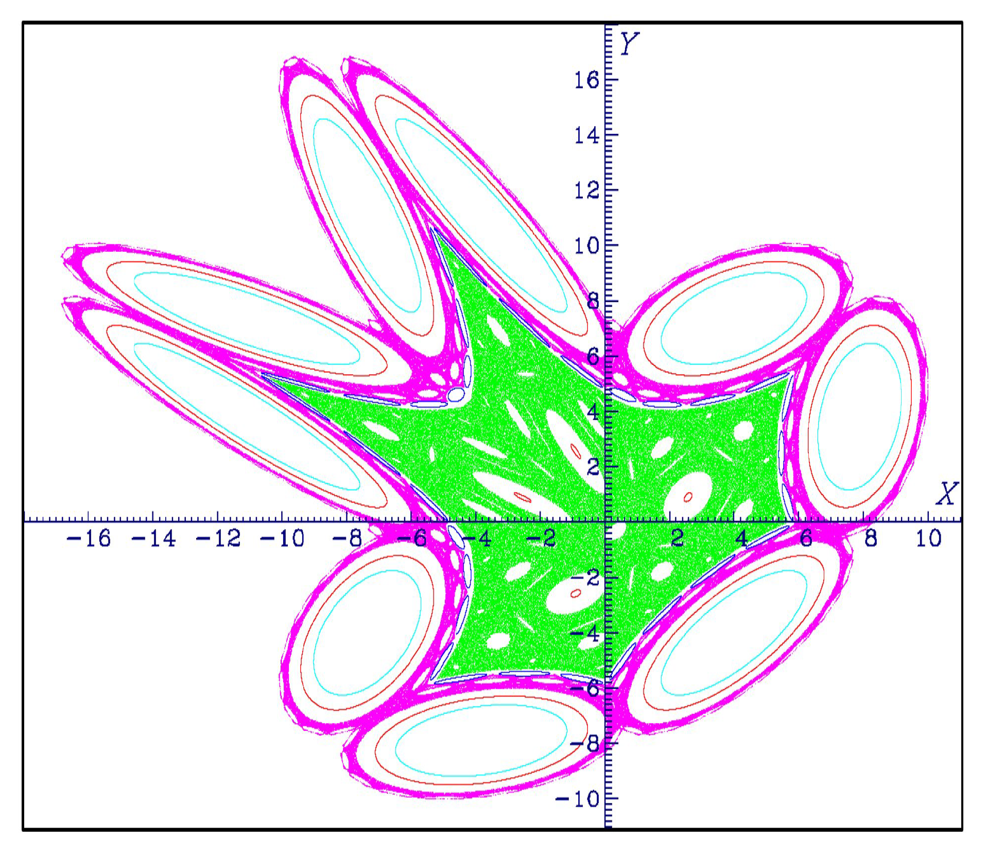
2.4. Chaotic Properties of the Conservative Map (|b| = 1)

In the conservative case (called the area-preserving case) $measure\left(f\right(\Delta \left)\right)=measure(\Delta )$, there is no attractor.

In addition to the analysis of Sushko et al. [18] (see Section 2.3), this conservative map has been studied by Lopesino et al. in [31], who proved that when $a>4$, a chaotic saddle exists in the square

$${\mathcal{S}}_q=\left\{(x,y)\in {\mathbb{R}}^2\left|\left|x\right|\le R,\left|y\right|\le R\right.\right\}$$

with

$$R=R\left(a\right)=\frac{a}{4(a-2)}.$$

(10)

The conservative case was studied by Li et al. [32], who highlighted that it can generate initial values-related coexisting infinite orbits. Its moving orbits are extremely dependent on its initial values, and present periodic, quasi-periodic, and chaotic orbits with different types and topologies. That means that the emergence of extreme multistability appears in the area-preserving Lozi map.

As an example, several such orbits are plotted in Figure 7. Li et al. noted that the coexistence of double or multiple attractors has been found in the Hénon map, the M-dimensional nonlinear hyperchaotic model [33], and multistage DC/DC switching converters [34]. Two types of simple 2D hyperchaotic maps with sine trigonometric nonlinearity and constant controllers were shown to generate initially boosted infinite attractors along a phase line [35,36]. Recently, a simple two-dimensional Sine map was presented to obtain infinitely many initially boosted attractors along a phase plane [37]. However, the authors emphasized that all these newly presented discrete maps only exhibit coexisting attractors with different positions. It can be remarked that coexisting infinite attractors with different topologies and different positions in the discrete maps, such as those in the area-preserving Lozi Map, have rarely been reported.

Li and Gu [38] studied the hierarchical structure of a chaotic sea and the existence condition and delimitation method of island chains for this map. They found the cause of the formation of two types of island chains associated with the elliptic period. The type of island chain depends on the rotation number of the linear matrix that defines the composite mapping (corresponding period).

2.5. Fractional Lozi Map

During the last four decades, the Lozi map has been generalized in many ways (for a survey, see [2]). Only its generalizations in the recent paradigm of fractional mappings are reported here, as this is a natural extension of the theory of fractal ordinary differential equations; in this context, the fractional Lozi map is used for electrical devices called memristors (see Section 3.3.2).

2.5.1. Classic Fractional Lozi Map

The first published example of fractional map used a constant fractional order $\nu$.

Using the Caputo-like delta difference

$$\begin{array}{ccc}\hfill & {}^c{\Delta }_a^{\nu }X\left(t\right)& ={\Delta }_a^{-(n-\nu )}{\Delta }^{n}X\left(t\right),\hfill \\ \hfill & & =\frac{1}{\mathrm{\Gamma }(n-\nu )}\sum _{s=a}^{t-(n-\nu )}{(t-s-1)}^{(n-\nu -s)}{\Delta }^{n}X\left(t\right),\hfill \end{array}$$

Khennaoui et al. [39] defined the fractal Lozi map as follows:

$$\left\{\begin{array}{ccc}\hfill & {}^c{\Delta }_a^{\nu }x\left(t\right)& =\alpha \left|x(t-1+\nu )\right|+y(t-1+\nu )+1-x(t-1+\nu ),\hfill \\ \hfill & {}^c{\Delta }_a^{\nu }y\left(t\right)& =\beta x(t-1+\nu )-y(t-1+\nu ),\hfill \end{array}\right.$$

(11)

for $0<\nu \le 1$ and $t\in {\mathbb{N}}_{a+1-\nu }=\left\{a+1-\nu ,a+2-\nu ,\dots \right\}$. In this example the fractional order of the two fractional differences is identical. This system is commonly referred to as a commensurate system. The following equivalent discrete integral equation of such a map can be obtained:

$$\left\{\begin{array}{ccc}\hfill & x\left(t\right)& =x\left(a\right)+\frac{1}{\mathrm{\Gamma }\left(\nu \right)}\sum _{s=a+1}^{t-\nu }{(t-s-1)}^{(\nu -1)}\left[-\alpha \left|x(t-1+\nu )\right|+y(t-1+\nu )+1-x(t-1+\nu )\right],\hfill \\ \hfill & y\left(t\right)& =y\left(a\right)+\frac{1}{\mathrm{\Gamma }\left(\nu \right)}\sum _{s=a-\nu }^{t-\nu }{(t-s-1)}^{(\nu -1)}\left[\beta x(t-1+\nu )-y(t-1+\nu )\right],\hfill \end{array}\right.$$

(12)

where $\frac{{(t-s-1)}^{(\nu -1)}}{\mathrm{\Gamma }\left(\nu \right)}$ is the discrete kernel function

$$\frac{{(t-s-1)}^{(\nu -1)}}{\mathrm{\Gamma }\left(\nu \right)}=\frac{\mathrm{\Gamma }(t-s)}{\mathrm{\Gamma }\left(\nu \right)\mathrm{\Gamma }(t-s-\nu +1)}$$

and $a=0$ yields the numerical formula

$$\left\{\begin{array}{ccc}\hfill & x\left(n\right)& =x\left(0\right)+\frac{1}{\mathrm{\Gamma }\left(\nu \right)}\sum _{j=1}^n\frac{\mathrm{\Gamma }(n-j+\nu )}{\mathrm{\Gamma }(n-j+1)}\left[-\alpha \left|x(j-1)\right|+y(j-1)+1-x(j-1)\right],\hfill \\ \hfill & y\left(n\right)& =y\left(0\right)+\frac{1}{\mathrm{\Gamma }\left(\nu \right)}\sum _{j=1}^n\frac{\mathrm{\Gamma }(n-j+\nu )}{\mathrm{\Gamma }(n-j+1)}\left[\beta x(j-1)-y(j-1)\right].\hfill \end{array}\right.$$

(13)

Extended numerical simulations of this fractional map have shown that the value of the fractional order $\nu$ modifies the general shape of the bifurcation diagram (compared to the non-fractional map) as well as the length of the chaotic interval. If $\nu =0.98$, the bifurcation diagram appears similar the corresponding integer diagram, with the exception of a small widening in the interval where chaos is observed. For smaller values of $\nu$, when $0\le \alpha \le 0.5$ the orbit no longer goes to a fixed point, unlike the non-fractional map. In fact, as n increases it can be observed that the trajectory becomes unbounded. A major difference between the bifurcation diagram of the integer and fractional maps concerns the interval over which chaos is observed, which becomes slightly smaller as $\nu$ decreases.

Ibrahim and Baleanu [40] used linear interpolation of quadratic and absolute value functions to define and study a combined Hénon–Lozi fractional map.

2.5.2. Variable Fractional Lozi Map

Several authors, including Al-Saidi et al. [41], have extended the definition of a fractional map to the case where the order of derivation is variable. To this end, they considered the function $\zeta \left(\nu \right)$ instead of $\nu$ in Section 2.5.1:

$$\begin{array}{ccc}\hfill & {}^c{\Delta }_a^{\zeta \left(\nu \right)}X\left(t\right)& ={\Delta }_a^{-(n-\zeta (\nu \left)\right)}{\Delta }^{n}X\left(t\right),\hfill \\ \hfill & & =\frac{1}{\mathrm{\Gamma }(n-\zeta (\nu \left)\right)}\sum _{s=a}^{t-(n-\zeta (\nu \left)\right)}{(t-s-1)}^{(n-\zeta (\nu )-s)}{\Delta }^{n}X\left(t\right)\hfill \end{array}$$

Hence, the variable fractional Lozi map (VFLM) is defined as

$$\left\{\begin{array}{ccc}\hfill & {}^c{\Delta }_a^{\zeta \left(\nu \right)}x\left(t\right)& =\alpha \left|x(t-1+\zeta (\nu \left)\right)\right|+y(t-1+\zeta \left(\nu \right))+1-x(t-1+\zeta \left(\nu \right)),\hfill \\ \hfill & {}^c{\Delta }_a^{\zeta \left(\nu \right)}y\left(t\right)& =\beta x(t-1+\zeta (\nu \left)\right)-y(t-1+\zeta (\nu \left)\right),\hfill \end{array}\right.$$

(14)

and for numerical values, when $a=0$ we obtain

$$\left\{\begin{array}{ccc}\hfill & x\left(n\right)& =x\left(0\right)+\frac{1}{\mathrm{\Gamma }\left(\zeta \right(\nu \left)\right)}\sum _{j=1}^n\frac{\mathrm{\Gamma }(n-j+\zeta (\nu \left)\right)}{\mathrm{\Gamma }(n-j+1)}\left[-\alpha \left|x(j-1)\right|+y(j-1)+1-x(j-1)\right],\hfill \\ \hfill & y\left(n\right)& =y\left(0\right)+\frac{1}{\mathrm{\Gamma }\left(\zeta \right(\nu \left)\right)}\sum _{j=1}^n\frac{\mathrm{\Gamma }(n-j+\zeta (\nu \left)\right)}{\mathrm{\Gamma }(n-j+1)}\left[\beta x(j-1)-y(j-1)\right].\hfill \end{array}\right.$$

(15)

Al-Saidi et al. studied the partial dynamics of such VFLMs. Additionally, they looked into the prerequisites that the variable fractional dynamic systems must meet in order to be stable and asymptotically stable. To obtain stable and asymptotically stable zero solutions, they imposed several essential requirements on the VFLM. To stabilize the system, they suggested combining these maps with control rules.

2.5.3. Complex Fractional Map

Other authors, such as Joshi et al. [42], have considered the definition of a fractional map (13) for the case where the order of derivation $\nu$ is a complex number with $0<Re\left(\nu \right)<1$. They used $L_1$ to denote the model defined by (13) and $L_2$ to denote the one defined by

$$x\left(n\right)=x\left(0\right)+\frac{1}{\mathrm{\Gamma }\left(\nu \right)}\sum _{j=1}^n\frac{\mathrm{\Gamma }(n-j+\nu )}{\mathrm{\Gamma }(n-j+1)}\left[-\alpha \left|x(j-1)\right|+x(j-1)+1-bx(j-2)\right].$$

(16)

To systematically investigate the impact of complex order on fractional maps, they set $\nu ={\nu }_0{e}^{ir\pi /2}$ with $0<{\nu }_0<1$, which reduces to the real fractional order for $r=0$. They studied the bifurcation diagram numerically, comparing it to the bifurcation diagram of the Hénon map.

In the case of the Hénon map, they did not observe chaos for $r\ne 0$, indicating that the chaotic attractor is destroyed when complex order was introduced. They checked their results using a number of different initial conditions, finding that the bifurcation diagram does not change, which highlights that multistability is not very pronounced for the fractional order.

They found, however, that the situation is different for the Lozi map. In this case, the chaos does not disappear. They computed the bifurcation diagrams of the Lozi map for ${\nu }_0=0.8$ and $r=0,0.01,0.1,0.5$ for model $L_1$.

The range of variable values indicates that there are parameter zones that are chaotic, or at least periodic with a very large period. They performed other tests as well, such as finding the largest Lyapunov exponent for models $L_1$ and $L_2$ to confirm the presence of chaos (the divergence of trajectories is exponential in the $L_1$ formulation, and the calculation of the Lyapunov exponent is justified). They found that the largest exponents are $0.264$ for model $L_1$ and $0.326$ for model $L_2$ for the parameters mentioned above. These results confirm that the Lozi map shows chaos for the difference equation of the complex fractional order.

Moreover, they noted that extremely strange bifurcations are observed in model $L_1$, showing bifurcation diagrams for $\nu =0.4+0.3i$ and $\nu =0.4+0.5i$ (see Figure 7a,b of [42]) which clearly indicate the possibility of very large periods and a rich bifurcation structure that is not generally seen in integer-order systems.

In addition, they noted that the system has memory; the complex fractional ordered Lozi map shows multistability, and the asymptotic attractor depends on the initial conditions.

Finally, they studied control (see Section 5.2.1) and synchronization (see Section 7.1.6) for this map.

3. The Use of the Lozi Map in Electrical Devices, Memristors, and Computers

The first paradigm change in the study of the Lozi map came in 1987, nine years after the initial publication. Instead of focusing on the theoretical study of its mathematical properties or on finding generalizations, electrical engineers used it to build new devices. Subsequently and continuing up to the present day, this map has been continuously involved in the field of electronics, electrical devices, multiple access communications, memristors, and computer software.

3.1. Chaos from Switched-Capacitor Circuits

Prior to 1990, computers were not as efficient as they are today, and many experimenters used analog electrical systems to explore the behavior of chaotic maps. In 1987, Rodriguez-Vasquez et al. [43] presented a special-purpose analog computer made of switched capacitor circuits for analyzing chaos and bifurcation phenomena in nonlinear discrete dynamical systems modeled by discrete maps. They published results for four maps: the logistic map, a piece-wise linear map

$$x_{n+1}=V-(\left|x_n\right|-0.4)\left[1+sgn(\left|x_n\right|-0.4)\right],$$

(17)

where $x\in \left[-4,4\right]$ for $0\le V\le 4$, the Hénon map (2), and the Lozi map (3) in the form

$$\left\{\begin{array}{c}{x}_{n+1}=3-1.8\left|x_n\right|+y_n,\hfill \\ y_{n+1}=0.25x_n.\hfill \end{array}\right.$$

(18)

For (18), they built a rather complicated circuit realization (see Figure 25 of [43]) and compared the attractor measured from this circuit with the corresponding numerical simulation, finding good agreement between them. Even if this example is not, strictly speaking, an application of the Lozi map for electrical purposes, it constitutes one of the first examples of solid realization. The same year, Matsumoto [44] considered a generalization of this map (similar to, though less general, than the one studied by Glendinning and Simpson [19]) and built an electric circuit to study its attractors.

3.2. Multiple Access Communication Based on Control of Special Chaotic Trajectories

In 2000, Dmitriev et al. [45] discussed the principle of multiple access in satellite communication systems or cellular telephony based on the fine structure of chaotic attractors and using control of special chaotic trajectories. They demonstrated the experimental verification of the proposed approach for asynchronous packet data transmission. In their approach, they considered that a chaotic attractor can be treated as a number of countable sets of special trajectories consisting of unstable periodic orbits (UPO) and transitions between these orbits. The instability of the periodic orbits and transient trajectories between them gives rise to irregular chaotic behavior. They used the set of the unstable “skeleton” periodic trajectories, constituting the structure of the strange attractor (or a part of this set), as a “reservoir” of potential codes for multi-user communication systems. They observed that the multitude of codes from a certain “reservoir” for communications is practically infinite, i.e., the number of users that can be provided with individual code sets is unlimited.

The initial information carrier (in the absence of the transmitted message) is the chaotic oscillations produced by the dynamic system. The “user” codes are the fragments of the entire complex motion; thus, each user’s “own” code does not disturb the system behavior, and alternating the “owned” code for a certain user and others’ orbits does not change the structure of the total signal in the channel. The signal in the channel is the “information for everybody”, containing pieces of chaotic trajectory, “owned” unstable cycles (orbits) and codes belonging to “others”. This means that the proposed method for the transmitted message formation additionally has the useful property of confidentiality. As both the position and duration of the code packages in the channel can be arbitrary, a sequential asynchronous stream of cycle-codes is realized.

As an example of the realization of their method, they considered twenty period-16 (UPO) of the Lozi map (3) for $a=1.7$ and $b=0.5$. They displayed the switching between them in the Figure 2 of [45] and showed from this diagram that the forming of all successive cycles (repeating ten times) is practically instantaneous. Improving on their initial method, they remarked that unstable periodic orbits can be utilized for encoding the entire transmitted information as well as to attribute it to this or that group of users, i.e., playing the role of “chaotic markers”. The idea of using the system of unstable periodic orbits as markers was applied to the problem of asynchronous packet transmission of data from several users through a single common communication channel.

They concluded that the generation and control of UPO may be realized in the relatively high-frequency bands provided by modern digital methods.

They later carried out a similar study with the Lozi map (3) for $a=1.4$ and $b=0.3$ in [46].

3.3. Memristors

In 1971, L.O. Chua predicted the existence of a missing fourth passive circuit element in addition to the three classical ones (resistors, inductors, and capacitor) [47]. He called these new elements ‘memristors’, referring to a resistor with memory. Memristors are characterized by a nonlinear constitutive relationship between the charge q and flux $\phi$. A physical device was not reported until 2008, when a physical model of a two-terminal hp device behaving as a memristor was announced [48]. This sparked intense research interest, with thousands of papers being published to date. A generalized version of Ohm’s law for theorizing about such devices was published ten years ago [49].

3.3.1. Memristor-Based Lozi Map with Hidden Hyperchaos

Nowadays, the discrete memristor model is a well known research hotspot. Many researchers have devoted themselves to the analysis of chaotic phenomena in discrete memristors. Recently, hidden attractors have been discovered in discrete memristor-based maps [50]. Wang et al. [51] included a discrete-time memristor to create a memristive Lozi map. This new 3D memristor-based Lozi map was established by coupling a discrete memristor to the original 2D Lozi map (3):

$$\left\{\begin{array}{c}{x}_{n+1}=1-a\left|x_n\right|+y_n,\hfill \\ y_{n+1}=b{x}_n+k{y}_{n}sin\left(z_n\right),\hfill \\ z_{n+1}=y_n+z_n,\hfill \end{array}\right.$$

(19)

where k is the real-valued control parameter coupling gain between the discrete-time memristor and the Lozi map.

Because there are no fixed points and hyperchaos can emerge, the memristor-based Lozi map is a hidden hyperchaotic map.

For certain specific control parameters, the 3D memristor-based Lozi map can show heterogeneous and homogeneous hidden multistability. It should be noted that heterogeneous hidden multistability implies the coexisting behavior of multiple hidden attractors of different stability types, while homogeneous hidden multistability indicates the coexisting behavior of multiple hidden attractors of the same stability type that only differ in dynamic intervals. In addition to the coexistence of these heterogeneous hidden attractors, the memristor-based Lozi map is very likely to produce the coexistence of homogeneous hidden hyperchaotic attractors, i.e., homogeneous hidden multistability. Therefore, the homogeneous hidden hyperchaotic attractors from the 3D memristor-based Lozi map can be robustly controlled by the memristor’s initial conditions.

Additionally, Wang et al. implemented this memristor in a digital circuit based on a high-performance microcontroller. They physically obtained an image of the hyperchaotic hidden attractors using a digital oscilloscope. Eventually, a digital platform was exploited and its experimental phase portraits were obtained to confirm the numerical portraits.

3.3.2. 3D Fractional Memristor-Based Lozi Map

Another method to obtain a memristor-based Lozi map is to consider the fractional counterpart of this map (see Section 2.5). Khennaoui et al. [52] used the Caputo-like delta difference to obtain the fractional map corresponding to (19):

$$\left\{\begin{array}{c}{\Delta }^{{\alpha }_1}{x}_n=1-a\left|x_n\right|+y_n-x_n,\hfill \\ {\Delta }^{{\alpha }_2}{y}_n=b{x}_n+k{y}_{n}sin\left(z_n\right)-y_n,\hfill \\ {\Delta }^{{\alpha }_3}{z}_n=y_n,\hfill \end{array}\right.$$

(20)

in which ${\Delta }^{{\alpha }_i}$$(i=1,2,3)$ stands for the Grunwald–Letnikov difference operator.

Obviously, when ${\alpha }_1={\alpha }_2={\alpha }_3=1$, the fractional map (20) corresponds to the first-order map (19).

This map exhibits hidden dynamic evolutions and multistability. The description of the fractional discrete memristor-based Lozi map was investigated according to its Lyapunov exponents, phase portraits, and bifurcation diagrams, demonstrating several kind of coexisting multiple hidden attractor behaviours that can be generated by the proposed model.

Using the classical discretization scheme, the iterative equation of the fractional order memristor-based Lozi map with no equilibrium point (20) is provided by

$$\left\{\begin{array}{c}{x}_{n+1}=1-a\left|x_n\right|+y_n+({\alpha }_1-1)x_n-\sum _{p_1=1}^n{\beta }_{p_1}{x}_{n-p_1},\hfill \\ y_{n+1}=b{x}_n+k{y}_{n}sin\left(z_n\right)+({\alpha }_2-1)y_n-\sum _{p_2=1}^n{\beta }_{p_2}{y}_{n-p_2},\hfill \\ z_{n+1}=y_n+{\alpha }_3{z}_n-\sum _{p_3=1}^n{\beta }_{p_3}{z}_{n-p_3},\hfill \end{array}\right.$$

(21)

where ${\beta }_{p_1}$, ${\beta }_{p_2}$, and ${\beta }_{p_3}$ are the binomial coefficients:

$${\beta }_{p_j=0}=-{\alpha }_1,{\beta }_{p_j}=\left(1-\frac{1+{\alpha }_j}{p+1}\right){\beta }_{p_{j-1}},j=1,2,3.$$

(22)

It can be shown that the value of ${\beta }_p$ decreases when the number of iterations p increases, regardless of the value of the fractional order. Thus, the easiest way to numerically implement the iteration Formula (21) is to use a finite truncation of the memory length M to approximate the fractional discrete memristor map (20). The short memory model M is provided by

$$\left\{\begin{array}{c}{x}_{n+1}=1-a\left|x_n\right|+y_n+({\alpha }_1-1)x_n-\sum _{p_1=1}^M{\beta }_{p_1}{x}_{n-p_1},\hfill \\ y_{n+1}=b{x}_n+k{y}_{n}sin\left(z_n\right)+({\alpha }_2-1)y_n-\sum _{p_2=1}^M{\beta }_{p_2}{y}_{n-p_2},\hfill \\ z_{n+1}=y_n+{\alpha }_3{z}_n-\sum _{p_3=1}^M{\beta }_{p_3}{z}_{n-p_3}.\hfill \end{array}\right.$$

(23)

The authors used a hardware platform based on a microcontroller (Arduino Uno board) to realize such a fractional memristive Lozi map for which the initial conditions can be changed easily. They showed that this map exhibits the initial condition-dependent dynamical phenomena of multistability and confirmed this through numerical simulations.

3.4. Chaotic Interleaver for Turbo Codes

In [53], Sahnoune and Berkani presented a new method to design a deterministic interleaver with random-like behavior based on the Lozi map. The interleaver is a fundamental part of turbo code design and plays a critical role in the performance of turbo coding. The basic role of the interleaver is to construct a random code and spread out burst errors. The interleaver provides “scrambled” information data to the second component encoder for constructing random codes, and decorrelates the inputs to the two component decoders; hence, the convergence of the iterative decoding algorithm improves.

An interleaver is a vector $\pi$, where $\pi \left(n\right)$ is the position in the information sequence that is interleaved to position n. Most proposed deterministic interleavers are linear interleavers with a designed index function provided by

$$\pi \left(n\right)=kn+umodN,0\le n\le N,$$

(24)

where k and n are fixed integers and k is prime relative to N.

The chaotic interleaver based on the Lozi map (with $a=1.7$ and $b=0.5$) is defined as follows:

• Step 1: the integer sequence ${\left\{n\right\}}_{n=1}^N\in \mathbb{Z}$ is mapped to a real number sequence ${\left\{x\left(n\right)\right\}}_{n=1}^N\in \mathbb{R}$ using (3).
• Step 2: ${\left\{x\left(n\right)\right\}}_{n=1}^N$ is mapped to another integer sequence ${\left\{s\left(n\right)\right\}}_{n=1}^N\in \mathbb{Z}$ by designing $s\left(n\right)$ as the position of index of $x\left(n\right)$ in the sort ascending of ${\left\{x\left(n\right)\right\}}_{n=1}^N$.
• Step 3: the chaotic interleaver indexes are provided by $\pi \left({\left\{s\left(n\right)\right\}}_{n=1}^N\right)={\left\{n\right\}}_{n=1}^N$.

Sahnoune and Berkani concluded that, compared with a random interleaver and dithered Golden interleaver, a chaotic interleaver has low latency, low complexity of implementation, and improves the security of the encoded data.

Urrea et al. [54] compared the performances of a chaotic interleaver with short block lengths to a new chaotic interleaver based on the Duffing map, which showed slightly better performance.

4. Applications in Optimization

Most engineering problems can be defined as optimization problems, e.g., finding an optimal trajectory for a robot arm, the optimal thickness of steel in pressure vessels, the optimal set of parameters for controllers, optimal relations or fuzzy sets in fuzzy models, etc. Solutions to such problems are usually difficult to find, and their parameters usually include variables of different types, such as floating point or integer variables.

Applications of the Lozi map in the now-flourishing field of optimization took longer to appear than applications in electrical devices. The main reason for this is due to a paradigm shift in optimization algorithms; instead of using deterministic algorithms such as gradient or steepest descent methods, which are not efficient in high-dimensional problem optimization involving hundred or thousand of variables, heuristic algorithms based on an imitation of Darwin’s theory of the evolution of species were introduced a few decades ago. Such algorithms require easy access to random or chaotic numbers. This is why interest has only recently focused on chaotic attractors.

Thirty years after the publication of the Lozi map, Araujo and Coelho used it as a core function for Particle Swarm Optimization (PSO) algorithms [55]. Their article was accepted on October 2007. Optimization algorithms based on chaos theory are methodologies for searching optimal solutions that differ from any of the existing traditional stochastic optimization techniques. Due to the wandering of chaos, it can carry out overall searches in the solution space at higher velocities compared to stochastic ergodic searches, which rely on probability-based computation. This remark appeared in the pioneering work of Caponetto et al. [56], who, four years before Araujo and Coelho, found that chaotic sequences improved the performance of evolutionary algorithms.

In fact, there are many kinds of genetic and evolutionary algorithms used for optimization; see [57] for a survey. In addition to PSO, Differential Evolution (DE) is a main branch of research into metaheuristic algorithms, and a few researchers have used the Lozi map [58]. Among the less conventional approaches for enhancing the performance of metaheuristics is the incorporation of chaos as a source of stochasticity. As a key operation in metaheuristics, stochasticity is typically used for three basic operators: selection, crossover, and mutation. It is possible to implement chaotic dynamics in any of these.

It should be noted that three years before Araujo and Coelho’s landmark publication, Zelinka et al. proposed a slightly different algorithm called SOMA (Self-Organizing Migrating Algorithm) using chaotic attractors, which can be classified among the metaheuristic algorithms [59].

Finally, the Lozi map is widely used in non-evolutionary chaotic optimization algorithms (see Section 4.5) such as the Improved Lozi map-based Chaotic Optimization Algorithm (ILCOA).

In this section, we explain how this chaotic map is used in these algorithms.

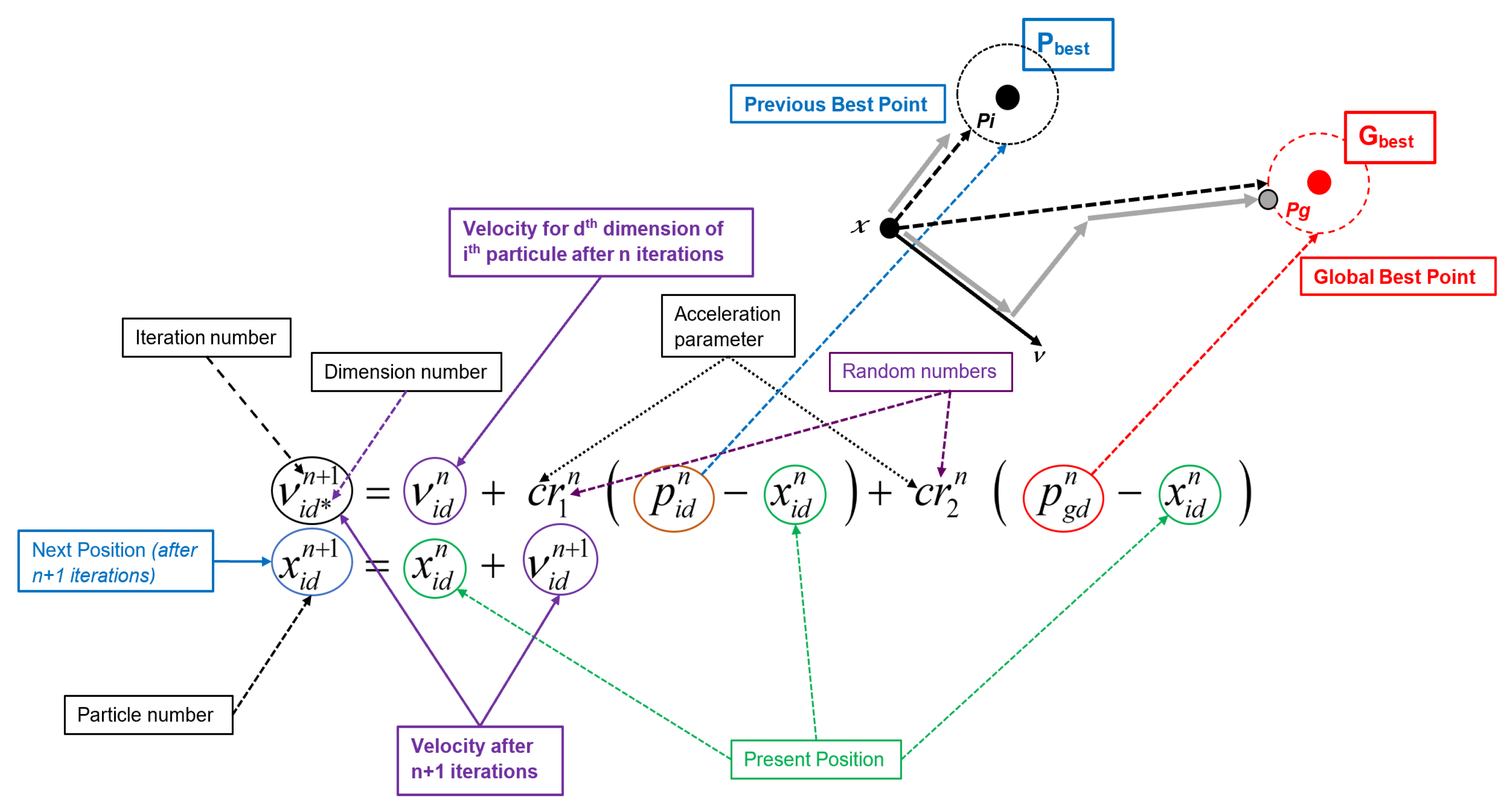
4.1. Particle Swarm Optimization (PSO)

Particle Swarm Optimization is a population-based evolutionary algorithm inspired by simulations of social behaviour instead of the survival of the fittest individual. PSO is randomly initialized with a population of individuals, which correspond to potential solutions. Unlike the most evolutionary algorithms, each particle in PSO is associated with a randomized velocity that “flows” through the problem space. In PSO, a uniform probability distribution is used to generate random numbers. However, the use of other probability distributions may provide improved fine-tuning or even allow the algorithm to escape from local optima, such as the distributions presented in [60]. In the meantime, the use of chaotic sequences has been proposed to generate random numbers for updating the velocity equation.

4.1.1. Thermal Vacuum System

In [55], the PSO approach was intertwined with Lozi map chaotic sequences to obtain a Takagi–Sugeno (TS) fuzzy model for representing dynamical behaviors. This proposed chaotic PSO (CPSO) approach was employed to optimize the premises in the IF–THEN rules of the TS fuzzy model, and were utilized in an experimental application, specifically, a thermal vacuum system employed for space environmental emulation and satellite qualification.

The essential idea of this model is to compute a global nonlinear model by partitioning the input space into fuzzy areas and approximating each area through a linear model.

The TS models consist of linguistic IF–THEN rules that can be represented by the following general form:

$$\left\{\begin{array}{c}{R}^{\left(j\right)}:IF\left(z_{1}is{A}_1^j\right)AND\cdots AND\left(z_{m}is{A}_j^m\right),\hfill \\ THEN{y}_j=b_0^j+b_1^j{x}_1^j+b_{q_j}^j{x}_{q_j}^j.\hfill \end{array}\right.$$

(25)

The IF statements define the premise part, while the THEN functions constitute the subsequent part of the fuzzy system; here, $A_i^j$ represents the labels of the fuzzy sets and $z={\left[z_1,z_2,\dots ,z_m\right]}^T$ with $i=1,\dots ,m$ is the input vector of premise p.

PSO is an optimization tool based on a population in which the position of each member particle is a potential solution to an analyzed problem. Each particle is associated with a randomized velocity that moves throughout the problem space. The coordinates of each particle are tracked in the problem space, and are associated with the best solution (fitness) achieved thus far. This value is called pbest. Another ‘best’ value that is tracked by the global version of the particle swarm optimizer is the overall best value. Its location, called gbest, can be obtained by any particle in the population. The past best position and the entire best overall position of the group are employed to minimize (maximize) the solution. At each time step, the PSO algorithm changes the velocity (acceleration) of each particle moving toward its pbest and gbest locations. Acceleration is weighted by random terms, with separate random numbers being generated for acceleration toward the pbest and gbest locations (see Figure 8).

Araujo and Coelho defined the following three CPSO approaches based on the Lozi map, considering that the velocity equation of each particle is updated at each step t by

$$v_i(t+1)=K\left[v_i\left(t\right)+c_{1}u{d}_i\left(t\right)(p_i\left(t\right)-x_i\left(t\right))+c_{2}u{d}_i\left(t\right)(p_g\left(t\right)-x_i\left(t\right))\right].$$

(26)

Approach 1 (CPSO1): the parameter $u{d}_i\left(t\right)$ is modified to

$$v_i(t+1)=K\left[v_i\left(t\right)+c_1{Y}_i\left(t\right)(p_i\left(t\right)-x_i\left(t\right))+c_{2}u{d}_i\left(t\right)(p_g\left(t\right)-x_i\left(t\right))\right].$$

(27)

Approach 2 (CPSO2): the parameter $u{d}_i\left(t\right)$ is modified to

$$v_i(t+1)=K\left[v_i\left(t\right)+c_{1}u{d}_i\left(t\right)(p_i\left(t\right)-x_i\left(t\right))+c_2{Y}_i\left(t\right)(p_g\left(t\right)-x_i\left(t\right))\right].$$

(28)

Approach 3 (CPSO3): the parameter $u{d}_i\left(t\right)$ is modified to

$$v_i(t+1)=K\left[v_i\left(t\right)+c_1{Y}_i\left(t\right)(p_i\left(t\right)-x_i\left(t\right))+c_{2}Y{}_i^{{}^{\prime }}\left(t\right)(p_g\left(t\right)-x_i\left(t\right))\right],$$

(29)

where $Y_i\left(t\right)$ are obtained from the chaotic attractor (3) with the parameter values $a=1.7$ and $b=0.5$ by scaling the variable $y\in \left[-0.6418,0.6716\right]$ within 0 and 1 at each iteration, as follows:

$$Y_i\left(t\right)=\frac{y_i\left(t\right)-\sigma }{\delta -\sigma },$$

(30)

with $\left[\sigma ,\delta \right]=(-0.6418,0.6716)$. The $Y{}_i^{{}^{\prime }}\left(t\right)$ are obtained in the same way as $Y_i\left(t\right)$, though with different initial values in (3). The constriction coefficient K is usually set to $K=0.729$.

After their launch and during their operational life, satellites are exposed to difficult physical conditions due to sunshine, albedo, earth radiation, and earthshine infrared in alternative shadow/eclipse conditions. In order to reproduce these challenging environmental conditions that satellites experience during their operational life as closely as possible, it is possible to use thermal vacuum chambers that consist of a chamber, a ‘shroud’ (set of pipes) which heats or cools off the environment, and auxiliary equipment. In the thermal vacuum system used by the Brazilian National Institute for Space Research (INPE), the original controller was designed to control the temperature on the shroud [61].

The three proposed approaches shown here have been tested thoroughly. The authors succeeded in eliciting a TS fuzzy model for this nonlinear and time-delay application, with the best algorithm obtained using COSP3.

4.1.2. Pid Controller Using PSO

A few years after the initial use of chaotic attractor properties in PSO by Araujo and Coelho, a team led by Ivan Zelinka from the Technical University of Ostrava (VSB-TU, Faculty of Electrical Engineering and Computer Sciences) extensively explored a quasi-similar method in a series of articles. They used a slightly different velocity equation, shown in Equation (26), introducing an inertia weight modification to the PSO strategy based on two control parameters, $w_{start}$ and $w_{end}$:

$$v_i(t+1)=w·v_i\left(t\right)+c_1·Rand·(pBest-x_i\left(t\right))+c_2·Rand·(gBest-x_i\left(t\right))$$

(31)

with (32)

$$w=w_{start}-\frac{\left(w_{start}-w_{end}\right)·t}{n}$$

(32)

where t stands for the current generation number and n for the total number of generations.

Within the Chaos PSO algorithm, the basic inbuilt computer random generator was replaced by a chaotic generator (in this case, using the Lozi map).

First, Pluhacek et al. [62] considered a Partial Integral Derivative (PID) controller for a Direct Current (DC) motor system in order to obtain optimal settings. A DC motor is any of a class of rotary electrical motors that converts direct current electrical energy into mechanical energy. Proportional Integral Derivative (PID) control is the most common control algorithm used by industry, and has been universally accepted in industrial control.

The popularity of PID controllers can be attributed to their robust performance in a wide range of operating conditions and their functional simplicity, which allows engineers to operate them in a simple and straightforward manner.

All PID controllers contain three unique basic coefficients, namely, proportional, integral, and derivative, which are varied to achieve optimal response (see [63] for a detailed description). A simplified form in the Laplace domain is provided by

$$G\left(s\right)=K\left(1+\frac{1}{s{T}_i}+s{T}_d\right),$$

(33)

where K is the controller gain, $T_i$ is the adjustable integral time parameter, and $T_d$ is the rate time. For suitable analytical calculations, the following form is often chosen:

$$G\left(s\right)=k_p+\frac{k_i}{s}+k_{d}s,$$

(34)

where the parameters are related to the standard form (33) through $k_p=K$, $k_i=K/T_i$, and $k_d=K/T_d$.

The transfer function for the DC motor considered in [62] is provided by

$$G\left(s\right)=\frac{0.9}{0.00105s^3+0.2104s^2+0.8913s}.$$

(35)

The optimization process involving the PSO algorithm was applied to minimize errors of the output transfer function, which can indicate the quality of regulation of the controller. Four criteria were considered:

-

The integral of the time multiplied by absolute error (ITAE):

$$I_{ITAE}={\int }_0^{T}t\left|e\left(t\right)\right|dt,$$

(36)

where $e\left(t\right)$ is the control error (see [63]).

-

The integral of the absolute magnitude of the error (IAE):

$$I_{IAE}={\int }_0^T\left|e\left(t\right)\right|dt.$$

(37)

-

The integral of the square of the error (ISE):

$$I_{ISE}={\int }_0^T{\left(e\left(t\right)\right)}^{2}dt.$$

(38)

-

The mean of the square of the error (MSE):

$$I_{MSE}=\frac{1}{n}\sum _{i=1}^n{\left(e\left(t\right)\right)}^2.$$

(39)

The presented data and graphical simulation results of [62] lend weight to the argument that the implementation of a chaotic Lozi map into the PSO algorithm as a random number generator can significantly improve its performance over other non-heuristic and heuristic methods when solving the problem of optimal PID controller design for DC motor systems.

In [64], the same authors addressed a fourth-order system provided by

$$G\left(s\right)=\frac{1}{s^4+6s^3+11s^2+6s}.$$

(40)

For statistical reasons, in both articles the optimization for each criterion was repeated thirty times. The results for the fourth-order system showed the same improvement of the Lozi map-based PSO method versus other non-heuristic and heuristic methods.

4.1.3. Assessment of Enhanced PSO Algorithm with Lozi Chaotic Map

In order to better evaluate the improvement conferred by the use of chaos in PSO algorithms, Pluhacek et al. [65], investigated the effect of tuning the control parameters a and b of (3) (recall that in all three above examples the parameter values were fixed to $a=1.7$ and $b=0.5$). Three different benchmark functions from the IEEE’s CEC 2013 benchmark suite [66] were selected for the tuning experiments. The controlling parameters of the Lozi map were set as follows:

$$\begin{gathered} a:1.3–1.7, \mathrm{step} 0.05 \\ b:0.1–0.6, \mathrm{step} 0.05 \end{gathered}$$

The benchmark functions were evaluated for dimension = 10, population size = 40, number of iterations = 2500, $w_{start}=0.9$, and $w_{end}=0.4$ according to the demands in [66]. The PSO algorithm with an adequately set Chaotic Pseudo-Random Number Generator (CPRNG) was run 100 times, and the mean results for each function and Lozi map setting were analyzed. The presented results support the claim that different settings of the chaotic map lead to significantly different CPRNG attributes, and have a great effect on the subsequent performance of the chaotic PSO algorithm. It seems that the most promising values for the parameter are $a\in [1.4–1.5]$ and $b\in [0.35–0.45].$

In [67,68], the authors compared the classical version of PSO with inertia weight (labelled PSO weight), PSO with Lozi map (PSO Lozi) with the sole classical value of the parameters $a=1.7$, $b=0.5$, and Differential Evolution (DE) with the “DE/Rand/1/Bin” strategy (see the next Section), for which they used four different benchmark functions in different dimensions:

-

The first De Jong function:

$$f\left(x\right)=\sum _{i=1}^{dim}{x}_i^2$$

(41)

-

The second De Jong function:

$$f\left(x\right)=\sum _{i=1}^{dim-1}100{\left(x_i^2-x_{i+1}\right)}^2+{\left(1-x_i\right)}^2$$

(42)

-

The Rastrigin function:

$$f\left(x\right)=10dim\sum _{i=1}^{dim}{x}_i^2-10cos\left(2\pi x_i\right)$$

(43)

-

The Schwefel function:

$$f\left(x\right)=\sum _{i=1}^{dim}-x_{i}sin\left(\sqrt{\left|x_i\right|}\right)$$

(44)

The basic PSO control parameters were set based on previous experiments and the literature, as follows: population size 30, iterations/generations 10 * the dimension, and dimensions of 2, 5, 10, 20, and 40.

For statistical reasons, optimization for each dimension value was repeated thirty times.

The numerical results with the first De Jong function highlighted that implementation of the chaotic number generator improved the performance of the PSO algorithm. The results were better or comparable with those of differential evolution. In the case of higher dimensions (20 and 40), DE provided better results, and the differences between the results of PSO Weight and PSO Lozi were less significant.

-

For the second De Jong function, PSO Lozi obtained the best results in almost all tests performed with this benchmark function. The performance of both PSO algorithms was better than that of DE.

-

In the case of Rastrigin’s benchmark function, there was no significant improvement in PSO performance; however, both PSO algorithms were significantly worse than DE for dim = 40.

-

The results for Schwefel’s function showed an increasing difference between the median values for PSO Weight and PSO Lozi, together with increasing dimension in favour of the PSO enhanced with the Lozi map. As in the previous case, both algorithms were surpassed by DE.

Pluhacek et al. deepened their previous analysis in [69], enlarging the tested population size from 30 to 50, 75, 100, 150, 200, 300, and 400. For smaller population sizes, they found similar results for the first and second De Jong functions as well as for the Rastrigin and Schwefel functions (for an example, see the case dim = 40 for the Second De Jong function in

Table 1. Results for the second De Jong function for dim = 40.

Result for dim = 40	PSO Weight	PSO Lozi	DE
The worst result	1.03$\times {\mathbf{10}}^{\mathbf{0}}$	$1.33\times {10}^0$	$1.34\times {10}^2$
The best result	$7.93\times {10}^{-2}$	2.25$\times {\mathbf{10}}^{-\mathbf{2}}$	$5.02\times {10}^1$
Median	$3.74\times {10}^{-1}$	2.19$\times {\mathbf{10}}^{-\mathbf{1}}$	$7.77\times {10}^1$

).

However, they found that increasing the size of the population led to significantly improved performance of both PSO algorithms with inertia weight (

Table 2. Mean value for thirty runs with Schwefel’s function, dim = 20, and generations = 200.

Pop. number	30	50	75	100	150	200	300	400
PSO Weight	−3697.6	−3873.6	−4141.0	−4255.8	−4329.6	−4866.4	−5316.4	−5377.7
PSO Lozi	−4340.1	−4560.4	−5032.8	−5241.8	−5802.0	−5998.1	−6174.6	−6225.6
DE	−6100.9	−5737.7	−5649.1	−5500.0	−5635.6	−5651.5	−5673.3	−5651.23

).

From this investigation, they concluded that the population size has very significant influence on both algorithms. With increasing population size, DE was outperformed by PSO even though both algorithms performed the same amount of CF evaluations.

Widening the scope of their investigations, in [70] Zelinka’s team explored two other chaotic maps: first, the dissipative standard map [71]

$$\left\{\begin{array}{c}{x}_{n+1}=x_{n+1}+y_{n+1}\left(mod2\pi \right),\hfill \\ y_{n+1}=b{y}_n+ksin{x}_n\left(mod2\pi \right),\hfill \end{array}\right.$$

(45)

with $b=0.6$ and $k=8.8$, and second, the Arnold’s Cat map [72]

$$\left\{\begin{array}{c}{x}_{n+1}=x_n+y_n\left(mod1\right),\hfill \\ y_{n+1}=x_n+k{y}_n\left(mod1\right),\hfill \end{array}\right.$$

(46)

with $k=0.1$. They compared these to the Lozi map with $a=1.7$ and $b=0.5$ using the same test function (41)–(44).

After a very extensive sequence of tests, they concluded that, first, the number generator based on the Arnold’s Cat chaotic map does not seem to have any significant effect on the behavior or performance of the PSO algorithm with linear decreasing inertia weight.

Second, the Lozi map used as the number generator seemed to have a significant positive effect on the speed of convergence of the algorithm. This may support the idea of using this modification in real-time optimization tasks on low-dimensional problems, especially because the risk of premature convergence and stagnation in higher dimensions seems to be a significant drawback of the PSO Lozi version. Finally, the PSO with the dissipative standard map seemed able to avoid premature convergence much better than any other version in this study. However, a drawback was its very slow speed of convergence; in other terms, a higher number of generations were needed to find the optimal value, or at least a satisfactory solution.

Finally, based on these conclusions, in [73] they found a new way to improve PSO based on the dissipative standard map and Lozi map by using them sequentially.

4.2. Differential Evolution (DE)

Meta-heuristic optimization methods have seen incredible advancements over the two last decades. More efficient computational algorithms have enabled solving of complex problems. One of these modern meta-heuristics is Differential Evolution (DE), an evolutionary computation method which has become widely used in engineering optimization due to its simple structure, ease of use, fast convergence speed, versatility, and robustness.

The main difference between genetic algorithms and DE is that in genetic algorithms mutation is the result of small perturbations to the genes of an individual (potential solution) while in DE mutation is the result of arithmetical combinations of individuals.

4.2.1. Overspeed Protection System of a Gas Turbine

In [58], dos Santos Coehlo considered the reliability–redundancy optimization problem of an overspeed protection system for a gas turbine. The fundamental idea behind DE is a scheme whereby it generates the trial parameter vectors. A DE population is subject to mutation, crossover, and selection operators. At each time step, DE mutates vectors by adding weighted random vector differentials to these operators. If the cost of the trial vector is better than that of the target, the target vector is replaced by trial vector in the next generation.

Among the many different strategies possible for DE, dos Santos Coehlo implemented the “DE/rand/1/bin” strategy, meaning that the target vector was randomly selected and only one difference vector was used. The bin acronym indicates that recombination was controlled by a binomial decision rule. Their strategy consisted of seven steps [58]

Step 1: Choice of the control parameters

Step 2: Initialization of population with M individuals

Step 3: Evaluation of individuals

Step 4: Mutation operation (or differential operation)

Step 5: Recombination operation

Step 6: Selection operation

Step 7: Verification of the stopping criterion

The mutation operation in Step 4 is an operation that adds a vector differential to a population vector of individuals according to

$$z_i(t+1)=x_{i,r_i}\left(t\right)+f_m\left(t\right)\left[x_{i,r_2}\left(t\right)-x_{i,r_3}\left(t\right)\right],$$

(47)

where $i=1,2,\dots ,M$ is the individual’s index of population; t is the generation (time), $x_i\left(t\right)={\left[x_{i_1}\left(t\right),x_{i_2}\left(t\right),\dots ,x_{i_n}\left(t\right)\right]}^T$ stands for the $i-th$ individual of a population of real-valued N-dimensional vectors, $z_i\left(t\right)={\left[z_{i_1}\left(t\right),z_{i_2}\left(t\right),\dots ,z_{i_n}\left(t\right)\right]}^T$ stands for the $i-th$ individual of a mutant vector, and $r_1$, $r_2$, and $r_3$ are mutually different integers that are different from the running index i, which is randomly selected with a uniform distribution from the set $\left\{1,2,\dots ,i-1,i+1,\dots N\right\}$. The mutation factor $f_m\left(t\right)>0$ is a real parameter which controls the amplification of the difference between two individuals with indexes $r_2$ and $r_3$.

It is well known that DE is particularly sensitive to its control parameters, particularly the mutation factor $f_m\left(t\right)$. In this context, due to the ergodic and dynamic properties of the Lozi map variables, dos Santos Coehlo introduced Lozi map-based DE (LDE), which can be useful in mutation factor design for escaping from local optima in optimization problems. The LDE approach was employed to increase the diversity of individuals’ population and prevent the premature convergence. The LDE approach is a modification of (47) provided by

$$z_i(t+1)=x_{i,r_i}\left(t\right)+L\left(t\right)\left[x_{i,r_2}\left(t\right)-x_{i,r_3}\left(t\right)\right],$$

(48)

where $L\left(t\right)$ is the Lozi map (3) normalized following (30) in the range $\left[0.1,0.9\right]$.

In each case study, fifty independent runs were carried out for each of the optimization methods involving fifty different initial trial solutions for each optimization method. Moreover, the DE and LDE approaches were adopted using 2250 cost function evaluations in each run. Both the DE and the LDE optimization methods were successfully applied to estimate the parameters of the overspeed protection system of a gas turbine in a reliability–redundancy optimization problem including discrete and continuous variables. Among seven variants of each of these methods, three DE variants and LDE five variants succeeded in finding the best solution for the tested methods. The author concluded that the LDE strategies have potential to be further applied in constrained optimization problems.

4.2.2. Chemical Reactor Optimization

Senkerik et al. used Differential Evolution in the optimization task of the batch reactor geometry [74]. The novelty of this approach is that Lozi map was not only used as a chaotic pseudo-random number generator to drive the mutation process as in [58], it was used for the crossover process in DE. The obtained results were compared with original reactor geometry and process parameters adjustment. The statistical analysis of the results provided by chaos-driven DE was compared with canonical DE strategy.

The authors used a simplified mathematical model of the reactor consisting of two physical inputs: one for chemical substances Chemical FK (Filter Cake), with parameters temperature $T_{FK}$, mass flow rate ${\dot{m}}_{FK}$, and specific heat $c_{FK}$, and one for the cooling medium of the temperature $T_{VP}$, mass flow rate ${\dot{m}}_V$, and specific heat $c_V$. The reactor had one output, with the cooling medium flowing through the jacket inner space of the reactor (with the volume related to the mass $m_{VR}$) and flowing out through the second output, with the following parameters: mass flow rate $m_V$, temperature $T_V$, and specific heat $c_V$.

There was an initial batch inside the reactor, with the mass parameter $m_P$ introduced at the beginning of the process. The chemical FK was then added to this initial batch, resulting in a reaction mixture inside the reactor with the following parameters: total mass m, temperature T, and specific heat $c_R$. In addition, the partially unreacted portions of the chemical FK were described by the concentration parameter $a_{FK}$.

This “batch” technique allowed for partial control of the temperature of the reaction mixture through controlled feeding of the input chemical FK. In general, this reaction is highly exothermic; thus, the most important parameter is the temperature of the reaction mixture. This temperature must not exceed $100{}^{\circ }$C because of safety and product quality requirements. The original design of the reactor was based on standard chemical–technological methods as part of a proposal involving the physical dimensions of the reactor and the parameters of the chemical substances. In the paper, these values were called the original parameters. The main objective of the optimization was to achieve the processing of large amounts of the chemical FK in a very short time. A system of four balance equations (49) was used to describe the reactor process, while another Equation (50) defined the term k:

$$\left\{\begin{array}{c}{\dot{m}}_{FK}=m^{\prime }\left[t\right],\hfill \\ {\dot{m}}_{FK}=m\left[t\right]a_{FK}^{\prime }\left[t\right]+km\left[t\right]a_{FK}\left[t\right],\hfill \\ {\dot{m}}_{FK}{c}_{FK}{T}_{FK}+\Delta H_{r}km\left[t\right]a_{FK}\left[t\right]=KS(T\left[t\right]-T_V\left[t\right])+m\left[t\right]c_R{T}^{\prime }\left[t\right],\hfill \\ {\dot{m}}_V{c}_V{T}_{VP}+KS(T\left[t\right]-T_V\left[t\right])={\dot{m}}_V{c}_V{T}_V\left[t\right]+m_{VR}{c}_V\left[t\right]T_V^{\prime }\left[t\right],\hfill \end{array}\right.$$

(49)

$$k=A{e}^{-\frac{E}{RT\left[t\right]}}.$$

(50)

Similar to dos Santos Coehlo [58], Senkerik et al. implemented the “DE/rand/1/bin” strategy; for the mutation operation, they used

$$u_{j,i,G_{+1}}=x_{j,r_1,G}+F·\left(x_{j,r_2,G}-x_{j,r_3,G}\right)$$

(51)

to minimize the cost function (CF)

$$f_{cost}=\sum _{t=0}^{t_1}\left|w-T\left[t\right]\right|+\sum _{t=0}^{t_1}{a}_{FK}\left[t\right]+pen.1+pen.2$$

(52)

with two penalizations:

$$pen.1=\left\{\begin{array}{c}0,Max\left(T\left[\tau \right]\right)\le 323.15,\hfill \\ 50,000else,\hfill \end{array}\right.$$

(53)

for $\tau \in (t_2,t_3)$ and

$$pen.2=\left\{\begin{array}{c}0,Max\left(T\left[\tau \right]\right)\le 373.15,\hfill \\ 50,000else,\hfill \end{array}\right.$$

(54)

for $\tau \in (0,t_3)$. The time intervals were set as follows: $t_1=15,000$ s, $t_1=20,000$ s, $t_1=25,000$ s.

The first penalization helps to find solutions in which the temperature of reaction mixture quickly cools down to its initial state, which shortens the process duration.

The second corresponds to the critical temperature. The best optimization results are shown in

Table 3. Statistical results of all 100 runs of Chaos DE and Canonical DE.

DE Version	Avg. CF	Median CF	Std. Dev.	Max CF	Min CF
Canonical DE	21,259.0	21,234.1	94.1	21,588.2	21,089.2
Chaos DE Lozi	21,107.6	21,107.4	25.4	21,160.7	21,059.0

and

Table 4. Average CF values for generation Nos. 50, 100, 150 and 200 from all 100 runs of Chaos DE and Canonical DE.

Generation No.:	50	100	150	200
Avg. CF for Canonical DE	25,320.1	22,719.9	21,619.8	21,259.0
Avg. CF for Chaos DE Lozi	24,707.1	21,992.1	21,265.2	21,107.6

. Their analysis showed that the temperature of the reaction mixture did not exceed the critical value. The maximum temperature was $373.11$ K ($99.95{}^{\circ }$C). The required temperature w used in the cost function was $370.0$ K ($96.85{}^{\circ }$C).

Senkerik et al. concluded that “based on statistical analysis, it is possible to claim that embedding the chaotic dynamics in the form of a chaotic pseudo-random number generator into differential evolution algorithm significantly improves the performance of DE.”

4.2.3. Evolutionary Chaos Control Optimization

An original study introduced by Zelinka’s team sought to utilize hidden chaotic dynamics in pseudo-random sequences generated via chaotic map to help the differential evolution algorithm search for the best controller settings for the same chaotic system. In [75,76,77], they considered (55) with the standard parameter values of $a=1.7$ and $b=0.5$, and tried to stabilize desired Unstable Periodic Orbits (UPO) using the chaos-driven DE for tuning the parameters of the Extended Delay Feedback (ETDAS) control method proposed by Pyragas [78].

$${\mathcal{L}}_{a,b}\left(\begin{array}{c}X\hfill \\ Y\hfill \end{array}\right)=\left(\begin{array}{c}1-a\left|X\right|+Y,\hfill \\ bX.\hfill \end{array}\right)$$

(55)

This control method takes the form

$$\left\{\begin{array}{c}{x}_{n+1}=1-a\left|X_n\right|+b{Y}_n+F_n,\hfill \\ F_n=K\left[\left(1-R\right)S_{n-m}-x_n\right],\hfill \\ S_n=x_n+R{S}_{n-m},\hfill \end{array}\right.$$

(56)

where K and R are adjustable constants which have to be evolutionary tuned, F is the perturbation, S is provided by a delay equation utilizing the previous states of the system, and m is the period of the m-periodic orbit to be stabilized. The perturbation $F_n$ in Equation (56) may have an arbitrarily large value, which can cause divergence of the system outside the output interval of the Lozi map system $\left[-1.4,1.4\right]$. Therefore, $F_n$ should have a value between $\left[-F_{max},F_{max}\right]$.

The suitable $F_{max}$ value was obtained from the evolutionary optimization process.

In these articles, two cost function designs, $C{F}_{SIMPLE}$ and $C{F}_{UNI}$, were utilized and compared. The goal of the first basic $C{F}_{SIMPLE}$, which can be used only for the stabilization of p-1 orbit, was to minimize the area created by the difference between the required state and the real system output on the whole simulation interval $\left[0,{\tau }_i\right]$:

$$C{F}_{SIMPLE}=\sum _{t=0}^{{\tau }_i}\left|T{S}_t-A{S}_t\right|,$$

(57)

where $T{S}_t$ is the target state and $A{S}_t$ the actual state.

Nevertheless, this simple approach has one prominent disadvantage, which is the inclusion of the initial chaotic transient behavior of the not-yet-stabilized system in the cost function value. To avoid this disadvantage, a universal cost function suppressing the initial chaotic transient behavior was introduced to ensure the stabilization of either the p-1 orbit (stable state) or the higher periodic orbit while retaining the possibility of adding penalization rules:

$$C{F}_{UNIVERSAL}=pe{n}_1+\sum _{t={\tau }_1}^{{\tau }_2}\left|T{S}_t-A{S}_t\right|,$$

(58)

where ${\tau }_1$ is the first minimal value of the difference between TS and AS and ${\tau }_2$ indicates the end of the optimization interval (${\tau }_1+{\tau }_s$), with $pe{n}_1=0$ if ${\tau }_i-{\tau }_2\ge {\tau }_s$ and $pe{n}_1=10\ast ({\tau }_i-{\tau }_2)$ if ${\tau }_i-{\tau }_2<{\tau }_s$ (i.e., late stabilization).

After hundreds of numerical tests, the researchers on Zelinka’s team concluded that embedding the chaotic dynamics into the differential evolution algorithm in the form of a chaotic pseudo-random number generator may help to improve their performance and robustness. In this way, optimal solutions were obtained securing very fast and precise stabilization for a convenient cost function surface in the $C{F}_{SIMPLE}$ case and a very chaotic and nonlinear cost function surface in the $C{F}_{UNIVERSAL}$ case.

4.2.4. Comparison of PSO with DE

Having presented the PSO and DE optimization methods, it is natural to compare them.

In [79], Senkerik et al. compared the swarm-based PSO technique to Differential Evolution on the task described above involving optimal evolutionary tuning of controller parameters for the stabilization of a Lozi discrete chaotic system. The novelty of this approach was that the most utilized examples of evolutionary/swarm based algorithms were compared directly on the highly nonlinear and complex multimodal optimization and simulation task. The simulations and comparisons were performed for three different required final behaviors of the chaotic system which were simulated in the following form:

• Case study 1: p-1 UPO, Lozi map as controlled system with $C{F}_{SIMPLE}$ (57)
• Case study 2: p-2 UPO with the same control
• Case study 3: higher order p-4 UPO with the same control

Within their research, a total of fifty simulations for each experiments was performed in the Wolfram Mathematica environment. All experiments used different initializations, i.e., a different initial population was generated in each run of DE/PSO.

The parameter settings for DE were population size = 25, F = 0.5, $Cr$ = 0.9, number of generations = 300, and CF Evaluations (CFE) = 7500.

For PSO, they were population size = 25, $c_1=c_2=2.0$, number of iterations = 300, and CF Evaluations (CFE) = 7500.

All simulations were successful and provided new optimal settings for the ETDAS control method, securing the fast stabilization of the chaotic system at the required behaviors, which were p-1 UPO (stable state), p-2 UPO (oscillation between two values), and p-4 UPO.

These results allowed the authors to compare DE and PSO in each case.

• Case Study 1: from the statistical point of view, the performance of both heuristics was similar. Nevertheless, DE converged towards the optimal solution in only twenty generations, and all fifty runs provided identical results. The convergence for PSO was much slower. Therefore, DE is more suitable for online control of nonlinear chaotic dynamics.
• Case Study 2: as in Case Study 1, the structure asnd simulation outputs showed similar features, with an even larger difference in favor of the DE algorithm.
• Case Study 3: dealing with the most complex and highly nonlinear dynamics, this case showed several interesting features. The classical geometrical (vector crossover)-based evolutionary algorithm was stacked in many suboptimal solutions, with only a small chance of leaving this area of the solution space. The PSO (swarm-based) algorithm was statistically better in the searching process, with a lower standard deviation and range of CF. Even when DE found a lower final CF value, PSO seemed to be a better and more robust choice for optimization in extremely nonlinear solution spaces due to its better natural exploration ability.

Senkerik et al. in [76] continued this comparison, using both $C{F}_{SIMPLE}$ and $C{F}_{UNIVERSAL}$:

• Case Study 4: p-1 UPO, Lozi map as controlled system with $C{F}_{UNIVERSAL}$ (58)
• Case Study 5: p-2 UPO with the same control
• Case Study 6: higher order p-4 UPO with the same control

The authors found that $C{F}_{UNIVERSAL}$ led to faster and more precise stabilization of the chaotic system.

4.2.5. Optimal Tuning of Speed Control for a Brushless DC Motor

As a last example involving the DE algorithm, we consider the work of Rodríguez-Molina et al. [80], who assessed the efficiency of the controller performance in a Brushless Direct current (BLDC) motor in an uncertain environment. The performance of the BLDC depends highly on the adaptability of the controller gains. The authors proposed a chaotic adaptive tuning strategy for controller gains (CATSCG) for speed regulation of BLDC motors. The CATSCG includes two sequential dynamic optimization stages based on identification and predictive processes, with a novel chaotic online differential evolution (CODE) used to provide the controller gain at each predefined time interval.

The CATSCG consisted of a two-stage tuning strategy; the dynamics associated with the future behavior of the BLDC motor are estimated in the first stage using the experience gained from the past optimization process. These dynamics are used in the second stage to find the controller gains that directly impact the closed-loop system responses through the novel Chaotic Online Differential Evolution (CODE) approach. Furthermore, CODE includes the Lozi chaotic initial populations in the differential evolution algorithm to enhance the diversity of candidate solutions in the dynamic environment, which further improves the quality of the controller gains under the effects of uncertainties.

The proposed chaotic online differential evolution (CODE) is an optimizer based on the DE/rand/1/bin variant of differential evolution (see Section 4.2.1). It incorporates a chaotic initialization and an elitist adaptation mechanism to improve the exploitative capacity and speed convergence of the original algorithm.

In the case of CODE, the random numbers utilized in the population initialization are generated by a Lozi chaotic map with $a=1.7$ and $b=0.5$. This is intended to increase the initial diversity of solutions at the beginning of each CODE run. Concerning the initial condition of the Lozi discrete dynamics adopted in the adaptive tuning proposal, it is established randomly at the very first instant of the control strategy execution (i.e., when $t=0$). After that, the Lozi map dynamics evolve one step forward each time a new chaotic random number is required (i.e., when it is required to generate a new random variable while generating each individual from the initial population of CODE).

Rodríguez-Molina et al.highlighted that among the tested optimizers (online differential evolution (ODE), online genetic algorithm (OGA), and online particle swarm optimization (OPSO)) in the adaptive controller tuning, the statistical results evidence that the use of CODE suitably balances the search capacities of exploration and exploitation of the algorithm such that the proposed CATSCG maintains the minimum possible motor velocity error under the effects of disturbances, uncertainties, noise, and reference velocity changes. They attributed the outstanding performance of CATSCG to the use of the chaotic initialization based on the Lozi map.

4.3. Self-Organizing Migrating Algorithm (SOMA)

In 2004, Zelinka introduced SOMA (Self-Organizing Migrating Algorithm) [59], a new class of stochastic optimization algorithms. Evolutionary algorithms work on populations of candidate solutions that are evolved in generations (i.e., two parents create one new individual, called the offspring) in which only the best-suited (or fittest) individuals are likely to survive. Instead, SOMA which can works on a population of individuals, is based on the self-organizing behavior of groups of individuals in a “social environment”, e.g., a herd of animals looking for food.

4.3.1. SOMA Philosophy

A group of animals such as wolves or other predators makes for a good example. If they are looking for food, they usually cooperate and compete such that if one member of the group is successful (has found food or shelter) then the other animals of the group change their trajectories towards the most successful member. If a member of this group is more successful than the previous best one (it has found more food, etc.), then again all members change their trajectories towards the new successful member. This is repeated until all members meet around one food source. This principle from the real world is of course strongly simplified; nonetheless, it can be said that it is the competitive–cooperative behavior of intelligent agents that allows SOMA to carry out very successful searches.

SOMA can be classified as an evolutionary algorithm, despite the fact that no new generations of individuals are created during the search based on philosophy of this algorithm. Only the positions of the individuals in the search space are changed during a generation, which is called a “migration loop”. Individuals are generated by random according to what is called the “specimen of the individual” principle. However, it is possible to classify SOMA as an evolutionary algorithm, as the final result after one migration loop is equivalent to the result from one generation derived by the classic EA algorithms.

Recently, Zelinka et al. used SOMA [81] for the design of quantum computing circuits for future quantum computers.

One key point in SOMA is the possibility of avoiding premature convergence by means of a so-called PRTVector (or Perturbation Vector), which limits the movement of particles to certain dimensions. Pluhacek et al. [82], considering that there is no conceptual barrier between DE, PSO, and SOMA, found that it is possible to noticeably improve the performance of a PSO algorithm driven by a Lozi chaotic map by implementing the PRTVector mechanism from the SOMA algorithm.

Through several examples of objective function, such as the Sphere function, Rosenbrock’s function

$$f\left(x\right)=\sum _{i=1}^{D-1}\left|100{(x_i^2-x_{i+1}^2)}^2-{(1-x_i)}^2\right|,$$

(59)

noise function, Rastrigin´s function (43), Schwefel’s function (44), Ackley’s function,

$$f\left(x\right)=-20exp\left(-0.2\sqrt{\frac{1}{D}\sum _{i=1}^D{x}_i^2}\right)-exp\left(\frac{1}{D}{\displaystyle \sum _{i=1}^D}{x}_i^{2}cos2\pi x_1\right)+20+e,$$

(60)

etc., they highlighted that it is possible to find better solutions even faster than with the original design of PSO driven by Lozi map.

4.3.2. Performance Comparison of PID Controller Using DE and SOMA Versus PSO

The comparison of PSO performance with DE (see Section 4.2.4) was extended to SOMA by Davendra et al. [63] for the problem of a PID controller (see Section 4.1.2) using three transfer functions:

• A third-order system

  $$G\left(s\right)=\frac{0.1}{s(3s+1)(0.8s+1)},$$

  (61)
• A fourth-order system comparable with the Ball and Hoop system (40),
• A third-order system for an electric DC Motor (35).

For all these problems, four unique optimization specifications (IAE (37), ISE (38), ITAE (36), and MSE (39)) were utilized. The obtained values were then used to calculate the following three performance indices:

• Rise time: the time it takes for the process output to achieve the new desired value. One-third of the dominant process time constant is typical.
• Settling time: the time it takes for the process output to die to between, say, $\pm 5\%$ of the setpoint.
• Peak overshoot: the magnitude by which the controlled “variable swings” past the setpoint $\pm 5\%–10\%$ overshoot is normally acceptable for most loops.

The Lozi map was selected as the chaotic map of choice due to its superior performance in previous research [83], in which additional comparisons for PID controllers using DE and PSO with the Lozi map can be found. The results obtained by chaos-driven DE and SOMA were compared with the values obtained using the Ziegler–Nichols method [84] and other published heuristics. For all the attempted problems, DE and SOMA performed better than the Ziegler–Nichols method. In the ball and hoop system (40), DE and SOMA performed better than the Genetic Algorithm (GA), while in the electric DC motor problem (35) they obtained better overshoot and settling times compared to other heuristics (GA, PSO, Continuous Cycling [85], and Evolutionary Programming [86]). The authors found that DE and SOMA both achieved consistently better results.

4.4. Other Genetic and Evolutionary Algorithms

In addition to PSO, DE, and SOMA there are a large number of other genetic and evolutionary optimization algorithms [57]. Among these, many use the Lozi map as a chaotic pseudo-random number generator. In this section, we describe several of these (for the tribes optimization approach, see Section 7.1.5).

4.4.1. Ant Lion Approach

The Ant Lion Optimizer (ALO) is a nature-inspired stochastic metaheuristic algorithm that mimics the hunting behavior of ant lions in nature. It uses the steps of hunting prey (such as a random walk of ants), building traps, entrapment of ants, catching prey, and rebuilding traps. This algorithm was proposed by Mirjalili [87] and adapted by Coelho et al. [88], who based it on the Lozi Map within the scope of Multiobjective Transformer Design Optimization.

Ant lions, or doodlebugs, belong to the Myrmeleontidae family and Neuroptera order (net-winged insects). The lifecycle of antlions includes two main phases: larvae and adult. A natural total lifespan can be up to three years, which mostly occurs in larvae (only 3–5 weeks for adulthood). Antlions undergo metamorphosis in a cocoon to become adults. They mostly hunt as larvae, with the adulthood period used for reproduction [87]. Their name originates from their unique hunting behaviour and favourite prey. An antlion larva digs a cone-shaped pit in sand by moving along a circular path and throwing out sand with its massive jaws. After digging the trap, the larva hides underneath the bottom of the cone and waits for insects (preferably ants) to become trapped in the pit. When the ant lion realizes that prey is in the trap, it tries to catch it. However, insects are usually not caught immediately, and try to escape the trap. In this case, the ant lion intelligently throws sand towards to edge of the pit in order to slide the prey to the bottom of the pit. When prey is caught in the ant lion’s jaws, the prey is pulled under the soil and consumed. After consuming the prey, the ant lions throws the remains outside the pit and repairs the pit for the next hunt.

The ant lion algorithm mimics the interaction between ant lions and ants in the trap. To model this interactions, ants are required to move over the search space and ant lions are expected to hunt them and become fitter using their traps. Because ants move stochastically in nature when searching for food, in the original ALO algorithm a random walk is chosen to model the ants’ movement. The steps of the ALO for single-objective optimization problems are briefly described in the following pseudo-code [88]:

• 1: Define the objective function and population size (NP)
• 2: Generate the populations of ant lions and ants
• 3: Evaluate the fitness of the ant lions
• 4: Initialize the generation counter $t=1$
• 5: For $t<maximumofiterations$:
• 6: For each ant from 1 to $NP$:
• 7:   Perform a random walk around a random ant lion,
• 8:   Perform a random walk around the elite individual (best ant lion),
• 9:   Update the position and check the search boundaries.
• 10:  Evaluate the fitness of the ants
• 11:  End for,
• 12:  Update ant lion positions based on the ants
• 13:  Update the elite individual and keep it in the population
• 14:  Update the generation counter $t=t+1$
• 15: End while,
• 16: Return the fittest (elite) ant lion.

On the other hand, multi-objective optimization refers to the optimization of more than one objective; these are generally in conflict with each other, resulting in no single solution to the problem. For this kind of optimization problems, the aim becomes to find good “trade-off” solutions that represent the best possible compromises among the objectives. The tradeoff between obtaining a well-converged and well-distributed set of Pareto-optimal solutions is an important issue in multi-objective optimization.

The MOALO is a classical multi-objective variant that uses the crowding distance [89] and the dominance concept for selecting the elite (best ant lion) and a tournament mechanism to select the ant lions to perform the random walk. One of the main pillars of optimization meta-heuristics, such as ALO, is their reliance on randomness or stochasticity, which is used to spark a path towards a desired goal. The current norm is the use of pseudo-random number generators. Unlike the MOALO, the proposed L-MOALO employs a mechanism with a chaotic dynamical behavior based on the Lozi map (similar to (30)) instead of pseudo-random number generators to enhance exploration during the ants’ movement.

The results of [88] obtained from simulations have shown that the MOALO and L-MOALO algorithms can be successfully applied to a Transformer Design Optimization (TDO) problem with two competing objectives, both providing a set of different solutions that present a trade-off between the objective costs.

4.4.2. Computational Intelligence Algorithm

Martinez-Vargas et al. [90] proposed a leader–follower optimization algorithm based on the combination of five different Population-based Algorithms (PAs) to tackle the high-dimensional optimization problem known as the Base Station (BS) deactivation problem in telephony. The general idea is to find the minimal set of active BSs in a 6G cellular network to maintain service for at least 99% of mobile users (MUs) who are reassigned due to BSs being shut down. Computational Intelligence (CI) is the key enabler for future 6G systems to autonomously manage their elements and build an intelligent wireless environment. The five follower PAs are: binary particle swarm optimization (BPSO), chaotic BPSO (BPSOC), a Genetic Algorithm (GA) with a steady-state population model (AGE), a GA with a generational model (AGG), and a binary artificial bee colony.

Each follower algorithm searches for its best solution (that is, the best local solution) in its set of candidate solutions during some number of iterations. Meanwhile, the leader algorithm checks whether the followers’ status is waiting or working. If the follower algorithms have the waiting status, the leader algorithm asks for the best local solution they have found thus far. Then, the leader gathers those best local solutions and chooses the best one among them as the best global solution. Consequently, the leader sets its status to working and sends the best global solution to the followers. When the followers receive the best global solution, they search for the worst candidate solution in their group of candidate solutions. The best global solution takes the place of the worst candidate solution (elitism). After the number of iterations is met, the leader resolves the problem, that is, it finds the lowest number of active BSs and reassigns those MUs whose BSs have been deactivated.

Among the follower algorithms, BPSOC has a unique mechanism to move through the search space. This mechanism uses chaos sequences to improve diversity and prevent premature convergence to a local optimum. To this end, BPSOC uses a Lozi map embedded in

$$v_{id}=\omega \ast v_{id}+c_1\ast v\ast \mathbf{chaos}\left(\right)\ast (g_{best}-x_{id})+c_2\ast \mathbf{chaos}\left(\right)\ast (p_{best}-x_{id}),$$

(62)

on the chaos() function.

The BPSO and BPSOC algorithms have exploitation bias. The diversity trend throughout iterations in these two followers is acute. This means that the convergence velocity towards $p_{b}est$ and $g_{b}est$ is fast. Furthermore, diversity is slightly greater in BPSOC because of the Lozi map effect (this is a unique mechanism in BPSOC).

In conclusion, Martinez-Vargas et al. found that the leader–follower optimization algorithm can find solutions even in challenging scenarios, and that BPSO and BPSOC find better solutions by performing deeper exploitation.

4.4.3. Mixed Fruit Fly Optimization

The Fruit Fly Optimization Algorithm (FOA) is a meta-heuristic technique proposed by Pan [91] that is inspired by the behavior of fruit flies. It simulates the foraging behavior of fruit flies. In comparison with other swarm intelligence-based algorithms, FOA has a sample framework with few parameters, and is easily understood and implemented. It has been improved as the Mixed Fruit Fly Optimization Algorithm LGM-FOA (Logistic Mapping-FOA) on the basis of the logistic map of Mitic et al. [92]; however, the algorithm shows an ideal state with respect to convergence precision and stability in the optimization process, as there are three discontinuous points from the logistic map. To solve this problem, Luo et al. [93] proposed a new mixed fruit fly algorithm that uses the Lozi map instead of the logistic map to conduct a global search for the optimal parameter values. It uses the value as the center to perform tiny fluctuations in order to obtain a final optimal value of quadratic optimization, thereby improving the initial value selection method of LGM-FOA. In support of the simulation between vector machine regression forecasting and the original Fruit Fly Algorithm, Particle Swarm Optimization (PSO), and LGM-FOA, this result testifies that the convergence accuracy of this new mixed fruit fly algorithm has obvious advantages.

4.4.4. Hybrid Chaos Immune Algorithm

Liu et al. [94], seeking to improve the performance of the immune algorithm, integrated chaos optimization into the immune clone selection algorithm. After decoding, a portion of the antibodies are mapped onto the Lozi system, then every optical value is collected at each iteration. Those values are added into the new antibody group to improve the antibody–antigen fitness value. Comparative results indicate that the optimization method of the hybrid chaos immune algorithm with self-adaptive parameter adjustment has many advantages, such as better self-adaptive capacity, higher computation efficiency, and better design accuracy.

4.5. Non-Evolutionary Chaotic Optimization Algorithms

In addition to evolutionary chaotic optimization algorithms, the Lozi map has been used as the core of more classical optimization algorithms.

4.5.1. Chaotic Optimization Algorithms

The tuning of PID controller (see Section 4.1.2 and Section 4.3.2) was addressed by Coelho [95] using a non-evolutionary chaotic optimization approach based on the Lozi map. He considered an automatic regulator voltage (AVR) system.

The problem of the dynamic stability of power systems has challenged power system engineers for decades. In a synchronous generator, the electromechanical coupling between the rotor and the rest of the system causes it to behave in a manner similar to a spring mass damper system, which exhibits oscillatory behavior around the equilibrium state following any disturbance, such as a sudden change in load, change in transmission line parameters, or fluctuations in the turbine output. Synchronous generator excitation control is one of the most important measures to enhance power system stability and to guarantee the quality of electrical power.

The transfer function of such a system is provided by

$$G\left(s\right)=\frac{0.07s+7}{0.0004s^4+0.0454s^3+0555sr+1.51s+8}.$$

(63)

The proposed chaotic optimization algorithm (CAO) (called the Chaotic Optimization Method based on Lozi map (COLM) by Coelho) is described as follows.

The Lozi map for this CAO is defined by

$$\left\{\begin{array}{c}{y}_1\left(k\right)=1-a\left|y_1(k-1)\right|+y(k-1),\hfill \\ y\left(k\right)=b{y}_1(k-1),\hfill \\ z\left(k\right)=\frac{y\left(k\right)-\alpha }{\beta -\alpha },\hfill \end{array}\right.$$

(64)

where k is the iteration number. Similar to (30), the values of y are normalized in the range $[0,1]$ to each decision variable in the n-dimensional space of the optimization problem. Thus, we have $y_1\in [-0.6418,0.6716]$ and $[\alpha ,\beta ]=[-0.6418,0.6716]$ for $a=1.7$ and $b=0.5$. Many unconstrained optimization problems with continuous variables can be formulated as the following functional optimization problem.

Find X to minimize $f\left(X\right)$, $X=[x_1,x_2,\dots ,x_n]$, where f is the objective function and X is the decision solution vector consisting of n variables. Here, $x_i$ bounded by lower limits $\left(L_i\right)$ and upper limits $\left(U_i\right)$. The COLM can be illustrated as follows.

Step 1: Initialization of variables and initial conditions. Set $k=1$, $y_1\left(0\right)$, $y\left(0\right)$ and set the

initial best objective function $\overline{f}$.

Step 2: Algorithm for chaotic global search.

 Begin

 While $k\le M_g$ do

   $x_i\left(k\right)=L_i+z_i\left(k\right)\times (U_i-L_i)$

   If $f\left(X\left(k\right)\right)<\overline{f}$  Then

     $\overline{X}=X\left(k\right)$

     $\overline{f}=f\left(X\left(k\right)\right)$

  End if

   $k=k+1$

  End while

  End

Step 3: Algorithm for chaotic local search.

  Begin

  While $k\le (M_g+M_L)$ do

    for $i=1$ to n

      If $r<0.5$ then (where r is a uniformly distributed random variable with

      range $[0,1]$)

         $x_i\left(k\right)={\overline{x}}_i+\lambda z_i\left(k\right)\times \left|U_i-{\overline{X}}_i\right|$

      Else

         $x_i\left(k\right)={\overline{x}}_i-\lambda z_i\left(k\right)\times \left|{\overline{X}}_i-L_1\right|$

      End if

    End for

    If $f\left(X\left(k\right)\right)<\overline{f}$ then

       $\overline{X}=X\left(k\right)$

       $\overline{f}=f\left(X\left(k\right)\right)$

    End if

     $k=k+1$

  End while

  End

Here, $M_g$ and $M_L$ are the maximum number of iterations of the chaotic global and local searches, respectively, while $M_g+M_L$ is the stopping criterion in iterations. The step size in chaotic local search is $\lambda$. The best objective function is $\overline{f}$, and $\overline{X}$ is the best solution from the current run of the chaotic search.

A suitable value for the step size usually provides a balance between global and local exploration abilities, and consequently a reduction in the number of iterations required to locate the optimum solution. In [95], the tested values of step size in COLM were described as follows:

• COLM(1): the step size $\lambda$ equals $0.01$
• COLM(2): the step size $\lambda$ equals $0.05$
• COLM(3): the step size $\lambda$ equals $0.10$
• COLM(4): the step size $\lambda$ linearly decreases from $0.10$ to $0.01$
• COLM(5): the step size $\lambda$ linearly increases from $0.01$ to $0.10$

In each case study, fifty independent runs were carried out for each of the COLM methods involving fifty different initial trial conditions $y1\left(0\right)$, $y\left(0\right)$.

From the case studies and comparison of the results through the five tested COLM approaches, it has been shown that the step size parameter $\lambda$ is essential to obtaining a good convergence profile. In this context, the $\lambda$ parameter regulates the trade-off between the global and local exploration abilities of the chaotic local search.

Shayeghi et al. [96,97], using the COA introduced by Coelho, proposed a multi-objective design for multi-machine Power System Stabilizers (PSSs). The PSS parameter tuning problem was converted to an optimization problem which was solved by COLM using the COLM(4) strategy. The authors suggested that COLM, which has the features of easy implementation, short execution time, and robust mechanisms of escaping from the local optimum, is a promising tool for engineering applications. The chaotic sequences increase its convergence rate and improve the precision of the results.

The effectiveness of the proposed method was tested on a multi-machine power system for a wide range of loading conditions and disturbances. Eigenvalues analysis provided the satisfactory damping level for the system modes, especially the low frequency modes, for systems with the proposed COA-based tuned PSSs, especially according to the time domain-based multi-objective function. Time domain simulations showed that the oscillations of the synchronous machines can be quickly and effectively damped for power systems over a wide range of loading conditions using the proposed PSSs.

The same authors used this algorithm for an output feedback damping controller design of a static synchronous compensator (STATCOM) [98].

The same algorithm was used by Jalilvand et al. [99] to design a Unified Power Flow Controller (UPFC) based on damping controllers using COA. Their eigenvalues analysis and simulation results showed that it has good performance for damping low-frequency oscillations and can improve transient stability under different operating conditions.

The COLM algorithm was later improved by Hamaizia and Lozi [100] by locally averaging the global search, then performing a few steps of chaotic local search around every point obtained by the chaotic series. In another study, Bououden and Abdelouahab [101] used transformations to modify the density of the Lozi map and combined Lozi and logistic maps during global and local search [102].

4.5.2. Improved Lozi Map-Based Chaotic Optimization Algorithm (ILCOA)

The COLM algorithm (called the Lozi Chaotic Optimization Algorithm (LCOA)) was improved by Alizadeh et al. in [103]. ILCOA was employed to solve a single-machine Power System Stabilizer (PSS) design problem, and its promising features in comparison with LCOA were highlighted.

In ILCOA, the chaotic variable interval is partitioned into three areas, namely, $A_1=[0,C_1]$, $A_2=[C_1,C_2]$ and $A_3=[C_2,1]$, in which $0<C_1<0.5$ and $0.5<C_2<1$ are adjustable parameters.

During the chaotic global search, each time a value of the chaotic variable $z_i$ is generated from the Lozi map and its validity is evaluated. If the chaotic variable $z_i$ belongs to $A_1$ or $A_3$, it must be regenerated; otherwise, it is reserved and used for calculating the objective function and checking its optimum, as it certainly belongs to the area $A_2$.

The lower ($L_i$) and upper ($U_i$) limits of the solution variables have been reformed as well. Thus, in the chaotic global search subroutine of ILCOA, $U_i$ and $L_i$ are replaced by $U_i^{new}$ and $L_i^{new}$, respectively, where

$$U_i^{new}=\frac{1-C_1}{C_2-C_1}{U}_i+\frac{1-C_2}{C_2-C_1}{L}_i,$$

(65)

$$L_i^{new}=\frac{-C_1}{C_2-C_1}{U}_i+\frac{C_2}{C_2-C_1}{L}_i,$$

(66)

$$z_i^{new}=\frac{1}{C_2-C_1}\times (z_i-C_1).$$

(67)

and where, similar to the chaotic global search subroutine, $C_1\le z_i\le C_2$; therefore, $0\le z_i^{new}\le 1$.

There is another parameter in the chaotic local search subroutine, namely, the step size $\lambda$, which is an important parameter in the convergence behavior of optimization methods. It adjusts small ergodic ranges around $\overline{X}$. The selection of the step size $\lambda$ has a direct effect on the process of generating a new trial solution. Balance between the global and local exploration abilities is provided by an appropriate value of $\lambda$. In [103], the authors introduced a new selection strategy for step size $\lambda$, namely, the semi-exponential step size (SESS), which focuses more on smaller values of $\lambda$ and contributes to better exploitation for refining the results:

$$\left\{\begin{array}{c}\lambda ={\lambda }_{max}-\frac{{\lambda }_{max}-{\lambda }_{mid}}{ite{r}_{max}^1}\times iteration,1\le iteration\le ite{r}_{max}^1\hfill \\ \lambda =\left[{\lambda }_{max}-\frac{{\lambda }_{max}-{\lambda }_{mid}}{ite{r}_{max}^1}\right]\times e^{\frac{(ite{r}_{max}^1-iteration)}{k}},ite{r}_{max}^1\le iteration\le ite{r}_{max}^2\hfill \end{array}\right.$$

(68)

where ${\lambda }_{m}ax$ is the initial step size, ${\lambda }_{mid}$ is the step size of the linear section ending, $ite{r}_{max}^2$ is the total number of searching generations in the local search subroutine, and ($ite{r}_{max}^2=M_L$) represents the generations in which the step size is linearly reduced. Different ending values of $\lambda$ can be achieved by adjusting k.

The results of the tests to solve a single-machine PSS design problem were promising, and showed that the ILCOA has features such as higher stability, better ability to escape from local minima, more robustness to search space size, and finer performance in comparison to LCOA, especially in high-dimensional problems with large search spaces.

In [104], Pourmousa et al. used ILCOA to evaluate the performance of photovoltaic panels. This evaluation inevitably involves having the exact model of solar cells. Different approaches to solar cell modeling have been proposed in the literature, and can generally be classified as either traditional or intelligent methods. To obtain an accurate model of such highly nonlinear systems, however, is a challenging task that continues to defy researchers. The authors suggested that the remarkable local and global search abilities of ILCOA grant it a distinct edge over other optimization methods, allowing it to sift through the entire search space for the global optimum. The efficacy of the proposed approach was highlighted by comparing its performance to those of three other algorithms: the Bird Mating Optimizer (BMO) [105], Improved Chaotic Whale Optimization Algorithm (ICWOA) [106], and LCOA in terms of Root Mean Square Error (RMSE), Relative Error, Mean Absolute Error (MAE), Normalized MAE, and Mean Bias Error.

The results showed that ILCOA performs better than the other algorithms and has higher convergence speed and stability. Moreover, it was able to reach a smaller value of the objective function compared with LCOA.

ILCOA was tested by Ebrahimi et al. [107] along with other algorithms to identify the parameter of the two chaotic Chen and Lorenz attractors as well as a permanent magnet synchronous motor system. Their simulation results ascertained the very good performance and high speed of this algorithm in identifying these systems in comparison with other algorithms.

5. Applications in Control Theory

Controlling chaos via different control schemes has received great interest after it was first introduced in 1990 by Ott, Grebogi, and Yorke [108]. The Lozi map is often used in this domain and in control theory-based chaos.

5.1. Observers

Observers are a primary tool used in control theory. Consider the problem of estimating the current state $x_k$ of a discrete-time nonlinear dynamical system described by a system of first-order difference equations:

$$\left\{\begin{array}{c}{x}_{k+1}=f\left(x_k\right),\hfill \\ y_{k+1}=h\left(x_k\right),\hfill \end{array}\right.$$

(69)

where, from past observations, $y_s$ and $s\le k$, where $k\in \left\{0,1,2,\dots \right\}$.

The vector fields $f:{\mathbb{R}}^n⟶{\mathbb{R}}^n$ and $h:{\mathbb{R}}^n⟶{\mathbb{R}}^p$ are continuous with $p\le n$. The variable $x\in {\mathbb{R}}^n$ stands for the state of the system, while the variable $y\in {\mathbb{R}}^p$ represents the measurement output.

An observer is a system driven by observations

$${\widehat{x}}_{k+1}=\widehat{f}({\widehat{x}}_k,y_k)$$

(70)

such that the error ${\tilde{x}}_k=x_k-{\widehat{x}}_k$ goes to zero as $k⟶\infty$.

In [109], Xiao provided a direct method for constructing a change of coordinates for the design of nonlinear discrete-time observers along with an explicit expression of this change of coordinates. He used the Lozi (3) and Hénon (2) maps to perform simulations for chaotic systems to illustrate the method.

Instead, Voortman et al. [110] designed a data rate-constrained observer for a dynamical system which functions in both discrete time and continuous time. The system is connected to a remote location by a communication channel that can transmit limited amounts of data per unit of time. The objective of the observer is to provide estimates of the state at the remote location through messages that are sent via the channel. The observer is designed such that it is robust to losses in the communication channel. It was tested through simulations for the Lozi map and the Lorenz system. As the Lozi map is not differentiable, a smoothed version was used:

$${\mathsf{\Phi }}_{\alpha }\left(\begin{array}{c}x\hfill \\ y\hfill \end{array}\right)=\left(\begin{array}{c}1-a{f}_{\alpha }\left(x\right)+by,\hfill \\ x,\hfill \end{array}\right),$$

(71)

where

$$f_{\alpha }\left(x\right)=\left\{\begin{array}{c}\left|x\right|,if\left|x\right|\ge \alpha ,\hfill \\ \frac{x^2}{2\alpha }+\frac{x}{2\alpha },if\left|x\right|<\alpha ,\hfill \end{array}\right.$$

(72)

with $\alpha <<1$.

By combining results from several other papers, the authors provided an analytical bound on the channel rate that depends on the Lyapunov dimension rather than the upper box dimension. These analytical bounds were computed for the smoothed Lozi map and the Lorenz system. Under the following Assumption 1, they proved Theorem 2 below.

Assumption 1. 

$a,b,\alpha >0$, $1-a<b<1$, $\alpha <{(a+1-b)}^{-1}$

Theorem 2 

([110]). Let Assumption 5 hold and let $S_0$ be a compact invariant set of the smoothed Lozi map (71). Then, the associated dynamical system is observable on the set $S_0$ via any communication channel with capacity

$$c<\frac{\left[2lo{g}_2\left(\frac{\sqrt{a^2+4b}-a}{2}\right)-lo{g}_{2}b\right]\left[lo{g}_2\left(\frac{\sqrt{a^2+4b}-a}{2}\right)\right]}{lo{g}_2\left(\frac{\sqrt{a^2+4b}-a}{2}\right)}.$$

In addition, they computed the Lyapunov dimension for the smoothed Lozi map. Simulations of the observer on both systems proved that the theoretical rate is closely related to the actual rate required to implement the observer.

5.2. Control of Chaos

In this section, we consider three aspects of the control of chaos: stabilization, adaptive and predictive control methods, and the identification of chaotic systems.

5.2.1. Stabilization of Chaos

Orbits of a dynamical system originating near an unstable fixed point remain unstable throughout the evolution of the system. To obtain regular motion from such initial point, the method used by Saha and Kumra [111] is to modify the value of the parameters a and b. As an example, they considered the case of $a=1.6$ and $b=0.5$ for which there exists an unstable fixed point $P^{*}=(0.47619,0.238095)$. Taking the initial point $P=(0.5,0.3)$ near $P^{*}$, they performed search using their previously defined method of asymptotic stability [112] for the new parameter values, for which the solution is periodic with the same initial point. This method is based on the computation of the Lyapunov exponents. They found that $a=1.52381$ and $b=0.57619$.

Gokce et al. [113] investigated the stability and tracking performance of discrete-time chaotic systems in the presence of external disturbance and noise. They developed a neural network control scheme on the basis of a novel adaptive learning rate to stabilize the chaotic motion of discrete-time chaotic systems to a fixed point as well as to track the desired reference trajectory. The effectiveness of the proposed method was investigated through simulation studies on the Lozi map and a performance comparison was made with the backstepping control strategy. The backstepping method based on the Lyapunov stability is a recursive procedure that breaks the full system into a sequence of small subsystems. Simulation studies demonstrated that the proposed method can successfully stabilize the chaotic trajectory of the system to the fixed point and track the desired reference trajectory. It has been shown that the proposed method is less sensitive to noise and disturbance and has a more robust property than the backstepping control scheme if the neural network is trained properly with accurate training parameters.

Joshi et al. [42] studied the control of a complex fractional-ordered Lozi map (see Section 2.5.2). They used the Pyragas method [78], which is a feedback method that can be attempted without any detailed knowledge of the dynamical system under consideration. There are two ways in which delay can be introduced in the system, are formulated as follows:

$$x\left(n\right)=\gamma x(j-2)+x\left(0\right)+\frac{1}{\mathrm{\Gamma }\left(\nu \right)}\sum _{j=1}^n\frac{\mathrm{\Gamma }(n-j+\nu )}{\mathrm{\Gamma }(n-j+1)}\left[-\alpha \left|x(j-1)\right|-x(j-1)+1+bx(j-2)\right],$$

(73)

and

$$x\left(n\right)=x\left(0\right)+\frac{1}{\mathrm{\Gamma }\left(\nu \right)}\sum _{j=1}^n\frac{\mathrm{\Gamma }(n-j+\nu )}{\mathrm{\Gamma }(n-j+1)}\left[-\alpha \left|x(j-1)\right|-x(j-1)+1+bx(j-2)+\gamma x(j-3)\right],$$

(74)

where $\gamma$ is the strength of the delay. For their numerical simulations, they set $\gamma =0.33$ for both (73) and (74).

They found that in both cases there is a reduction in the range over which chaos is observed. Period 2 is stabilized instead.

In Case 1 (73), Period 2 has an even more stable range, and the stability range of Period 1 is reduced, whereas for Case 2 (74) the range of Period 1 is significantly increased and that of Period 2 spans over a smaller range of parameters. Thus, chaos control can be achieved using the Pyragas method even in complex-order fractional maps.

5.2.2. Adaptive and Predictive Control

In [114], Chen and Dong presented interesting analysis and simulations on the control of chaotic dynamic systems using conventional feedback control strategies. The trajectories of the chaotic Lozi system are controlled to its equilibrium points using conventional feedback controls. The proposed controlled Lozi map is

$$\left\{\begin{array}{c}{x}_{k+1}=1-a\left|x_k\right|+y_k,\hfill \\ y_{k+1}=b{x}_k-K{v}_k.\hfill \end{array}\right.$$

(75)

For this system, Chen and Dong proved the following.

Proposition 2 

([114]). A necessary and sufficient condition for the local controllability of the chaotic Lozi system (3) to its equilibrium point $(x^{*},y^{*})=\left(\frac{1}{a-(b-1)},\frac{b}{a-(b-1)}\right)$ is $v_k⟶0$, as $k⟶\infty$, where $u_k=-K{v}_k$ is the feedback controller applied to the system shown in (75) and $v_k$ is the executive control input in the feedback $u_k=-K{v}_k$.

Computer simulations have been performed for $a=1.8$, $b=-1$, $K=-0.195$; $a=1.8$, $b=0.4$, $K=1.205$; $a=1.8$, $b=0.997$, $K=1.802$; and $a=1.8$, $b=1.0$, $K=1.805$.

Improving this method, Gonzalez [115] considered the Lozi map and showed that the trajectories can be driven to the fixed point as well as to other fixed reference points $(x^{*},b{x}^{*})$. The controlled the Lozi map defined as

$$\left\{\begin{array}{c}{x}_{k+1}=1-a\left|x_k\right|+y_k+u_k,\hfill \\ y_{k+1}=b{x}_k.\hfill \end{array}\right.$$

(76)

The following two control algorithms were proposed.

• Case 1: the value of a is unknown and the value of b is precisely known. In this case, the chosen control law is

  $$u_k={\tilde{a}}_k\left|x_k\right|-b{x}_{k-1}-1+x^{*},$$

  with

  $${\tilde{a}}_{k+1}={\tilde{a}}_k+\frac{\alpha \left|x_k\right|}{\gamma +x_k^2}\left(x_{k+1}-(-\tilde{a}\left|x_k\right|+b{x}_{k-1}+1+u_k)\right)$$

  and $\alpha >0$, $\gamma \ge 0$.
  With $a_k={\tilde{a}}_k-a$, the closed loop system emerges:

  $$\left\{\begin{array}{c}{x}_{k+1}=a_k\left|x_k\right|+x^{*},\hfill \\ a_{k+1}=a_k-\frac{\alpha {\left|x_k\right|}^2}{\gamma +x_k^2}{a}_k.\hfill \end{array}\right.$$
• Case 2: both values of a and b are known approximately. In this second case, the chosen control law is

  $$u_k={\tilde{a}}_k\left|x_k\right|-1+x^{*},$$

  (77)

  where the parameter estimator is provided by

  $${\tilde{a}}_{k+1}={\tilde{a}}_k+\frac{\alpha \left|x_k\right|}{\gamma +x_k^2}\left(x_{k+1}-(-\tilde{a}\left|x_k\right|+1+u_k)\right)$$

  (78)

  and $\alpha >0$, $\gamma \ge 0$.
  With $a_k={\tilde{a}}_k-a$ and $z_k=x_{k-1}$, the closed loop systems emerges:

  $$\left\{\begin{array}{c}{x}_{k+1}=a_k\left|x_k\right|+b{z}_k+x^{*},\hfill \\ z_{k+1}=x_{k-1},\hfill \\ a_{k+1}=a_k-\frac{\alpha {\left|x_k\right|}^2}{\gamma +x_k^2}({\tilde{a}}_k\left|x_k\right|+b{z}_k).\hfill \end{array}\right.$$

  (79)

In this case, there is now the law b. It was proved that for every real a and $-1<b<1/2$, $b\ne 0$ there exist $\alpha$ and $\beta$ such that the fixed point is asymptotically stable for (79). This means that by applying the adaptive strategy (77) and (78) to the control system (76) and taking $(x_1\left(0\right),x_2\left(0\right),{\tilde{a}}_0)$ in the neighborhood of $(x^{*},q{x}^{*},a-sgn\left(x^{*}\right)b)$, we obtain $(x_1\left(k\right),x_2\left(k\right))⟶(x^{*},q{x}^{*})$ as $k⟶+\infty$; at the same time, we obtain a better approximation to the values of a and b.

These two proposed control laws can be applied when $0<b<1$, $a>b+1$, and $2a+b<4$, that is, for the regions in the parameter space where chaos can occur (see Figure 3). It has been shown that when using these control laws $(x,y)$ converges towards $(x^{*},b{x}^{*})$.

In [116], Park et al. investigated the possibility of controlling discrete-time chaotic dynamical systems through a generalized predictive control (GPC) method which does not require a precise mathematical model of the chaotic dynamics. GPC methods may be considered as a kind of adaptive control strategy. By combining the ARMAX (AutoRegressive Moving Average model with eXogenous noise input) modeling with the GPC technique, they developed a strategy for adaptive control of uncertain discrete-time chaotic systems. They investigated both the control performance and the system’s sensitivity to initial conditions, and compared them with that of the conventional reference model adaptive control by means of numerical simulations on Lozi (for $a=1.8$ and $b=0.4$) and Hénon maps. Simulation results showed that this new controller yields faster settling time and more robust tracking performance.

For the same value of parameters of the Lozi map, Feng and Chen [117] have presented a new adaptive control algorithm. The basic idea behind their proposed approach is to represent the chaotic system as a Takagi–Sugeno fuzzy model (see Section 4.1.1), design a local linear adaptive controller in each local region, and then reassemble a global adaptive controller over the entire domain in such a way that the stability of the closed-loop adaptive control system is guaranteed.

5.2.3. Identification of Chaotic Systems

In [118,119], Chen et al. studied a feed-forward artificial neural network in a Wiener-type cascade dynamic model in which a three-layer feed-forward artificial neural network is employed as the nonlinear static subsystem and a simple linear plant is used as the dynamic subsystem. They presented theoretical results showing that various chaotic systems can be well identified by these two basic structures by training the neural network and choosing an appropriate linear subsystem. They demonstrated the approximation capability of the proposed system through simulations, where it was used to identify (synchronize) the chaotic continuous-time Duffing oscillator and the discrete-time Hénon and Lozi systems.

6. Cryptography

Cryptography is the primary means of protecting communications in the cyber-centric world in which humankind lives today. Modern technologies involve fast communication links between potentially billions of devices via complex networks (satellites, mobile phones, the internet, etc.). The primary concern posed by these complex and tangled networks is their protection against passive and active attacks that could compromise public safety and privacy. Cryptography has been around for over two thousand years, with the famous Caesar code being used by Emperor Julius Caesar. Today, the properties of chaotic attractors are recognized as the basis of many different methods of cryptography.

6.1. Theoretical Algorithms

The literature includes two articles in which the Lozi map is at the center of theoretical cryptographic algorithms. In the first considered article, Sira-Ramirez et al. [120] proposed the use of nonlinear exact chaotic system state reconstructors for the fast and efficient decoding of multiple discrete-time chaotic encrypted digital messages. After a general description of their method, in order to test the effectiveness of the exact reconstructor scheme in an actual message decoding problem, they applied it using the Lozi map. They considered transmission in a noise-free environment such as the internet.

They transmitted to a remote computer containing a reconstructor digital computer program, a message consisting of a digitized file of Van Gogh’s self portrait. The encoding of the messages was carried out using the states z and w of the following unobservable but constructible Lozi system:

$$\left\{\begin{array}{c}{x}_{k+1}=z_k,\hfill \\ z_{k+1}=-a\left|z_k\right|+b{x}_k+1,\hfill \\ w_{k+1}=x_k{z}_k,\hfill \\ y_k=x_k.\hfill \end{array}\right.$$

(80)

The exact reconstructor of system (80) for the non measured variable $z_k$ may be obtained trivially, as x is a one-step delay of z. This was readily derived to be

$$\left\{\begin{array}{c}{x}_k=y_k,\hfill \\ z_k=-a\left|y_k\right|+b{y}_{k-1}+1,\hfill \\ w_{k+1}=y_{k-1}(-a\left|y_{k-1}\right|+b{y}_{k-2}+1).\hfill \end{array}\right.$$

(81)

The image and text files were chaotically encoded in a byte-by-byte fashion after a simple normalization of the carrier chaotic states by an appropriate constant factor. Thus, they defined

$$I_k=K_1{z}_k+i_k,T_k=K_2{w}_k+t_k,i_k=I_k-K_1{\widehat{z}}_k,t_k=T_k-K_2{\widehat{w}}_k,$$

where $i_k$ and $t_k$ represent the kth byte of the image file, $I_k$ and $T_k$ are the corresponding kth bit of the chaotic encrypted image, and the factors $K_1$ and $K_2$ are suitable normalizing parameters, both taken as equal to 1000. The reconstructed states $\widehat{z}$ and $\widehat{w}$ exactly coincide with the original states z and w.

The encryption and decryption programs were written in the C programming language and compiled with Borland $C^{++}$ version 1.01. The size of the digital image file was approximately 120 KB. The process of encryption was completed in approximately two seconds, as was the decoding process.

In the second article, Aliwi and Ajeena [121] used an unconventional generalization of (3) based on the chaotic cosine map recently published in [122].

The Cosine Chaotic Map (CCM) is a chaotification method that enhances the chaotic complexity of existing chaotic maps. This method performs the cosine function alongside a chaotic map that cascades in the system under consideration. Thus, the results provide a new chaotic map having a wide chaotic range within the closed interval $\left[-1,+1\right]$. Theoretically, the CCM has properties based on the properties of the underlying seed maps. In the case of the Lozi map, Aliwi and Ajeena considered (3), changing 1 to 3 in the first component

$$f\left(\begin{array}{c}x\hfill \\ y\hfill \end{array}\right)=\left(\begin{array}{c}3-a\left|x\right|+y,\hfill \\ bx,\hfill \end{array}\right)$$

(82)

with $a=-1.8$ and $b=0.25$. Then, they inserted (82) in CCM:

$$f\left(\begin{array}{c}x\hfill \\ y\hfill \end{array}\right)=\left(\begin{array}{c}cos\left(2^{(k+3-a\left|x\right|+y)}\right),\hfill \\ cos\left(2^{(k+bx)}\right),\hfill \end{array}\right)$$

(83)

where $k\in \left[10,24\right]$.

Starting with any initial point $(x_0,y_0)$ belonging to the basin of attraction of the Lozi map, the iterates randomly fulfill the square ${\left[-1,+1\right]}^2$ (see Figure 9).

Based on a Knapsack problem approach, a fuzzy chaos-based cryptography method for a chaotic cosine map was proposed in which the system works by designing the Takagi–Sugeno (TS) fuzzy model (see Section 4.1.1) on a chaotic map as a seed map in the cosine map. The basic idea of this method is to apply the chaotification method in order to use a cosine chaotic map approach on the outputs of the TS fuzzy model to compute a real super-increasing sequence applied in the Knapsack equation. Aliwi and Ajeena [121] explicitly described this method, which is too long to be included here. The algorithmic performance of the method was derived as well. In addition, numerical simulations were presented to demonstrate the effectiveness of the proposed method.

6.2. Algorithms for Images

6.2.1. Image Encryption Algorithms

Several algorithms for image encryption based on the Lozi map have been developed.

An optical color image encryption scheme based on a fingerprint key and three-step phase-shifting digital holography was proposed by Su et al. [123]. In this scheme, the fingerprint directly serves as a secret key. The random phase masks generated from the fingerprint using a secure hash algorithm (SHA-256) and the chaotic Lozi map are used as interim variables. With the help of the fingerprint-based random phase masks located in the linear canonical transform domain and the three-step phase-shifting digital holography, the primary color image that is hidden in a grey-scale carrier image can be encrypted into three noise-like holograms. In addition, the parameters of the chaotic Lozi map and linear canonical transform can provide additional security to the proposed encryption scheme.

The generation process of the fingerprint-based random phase masks mainly comprises the following steps [123]:

•

Step 1: Calculate the hash value of the fingerprint using the SHA-256; a 256-bit hash value expressed as a hexadecimal number array can be obtained as follows: $H=\left[h_1,h_2,\dots ,h_{64}\right]$.

•

Step 2: Use elements of the array H to generate the initial values of the chaotic Lozi map in the following way:

$$\left\{\begin{array}{c}x=x_0+hexa2dec\left(H(h_i:h_{i+7})\right)\times {10}^{-16},\hfill \\ y=y_0+hexa2dec\left(H(h_i:h_{i+7})\right)\times {10}^{-16},\hfill \end{array}\right.$$

(84)

where $i,j=1,2,\dots 57$; $x_0$, $y_0$, and x, y denote the common and generated initial values of the chaotic Lozi map, respectively; and $hexa2dec\left(x\right)$ is used to convert hexadecimal number x to a decimal number.

•

Step 3: Suppose that the size of fingerprint-based random phase mask to be generated is $M\times N$ pixels. First, construct the chaotic Lozi map with initial values x and y, then iterate $\frac{M\times N}{2}$ times to obtain two random sequences $X=\left\{x_1,x_2,\dots ,x_{\frac{M\times N}{2}}\right\}$ and $Y=\left\{y_1,y_2,\dots ,y_{\frac{M\times N}{2}}\right\}$.

•

Step 4: Combine sequence X with sequence Y to form a new random sequence Z where $Z=\left\{x_1,x_2,\dots ,x_{\frac{M\times N}{2}};y_1,y_2,\dots ,y_{\frac{M\times N}{2}}\right\}$.

•

Step 5: Reshape the random sequence Z to form a two-dimensional random matrix $RM$ with size $M\times N$, where $RM=reshape(Z,M,N)$.

•

Step 6: The fingerprint-based random phase mask $FRPM$ can be generated in the following way: $FRPM=exp(i·\pi ·RM)$.

It is worth noting that a series of fingerprint-based random phase masks can be generated using different elements of the array H to generate the initial values of the chaotic Lozi map from Equation (84) and repetition of steps 3–6.

We do not describe the other parts of the algorithm that are not linked to the Lozi map here.

This algorithm was tested numerically with common initial values of $x_0=0.34$ and $y_0=0.0$ and the common control parameters $a=1.75$ and $b=0.33$. Numerical simulation results showed that the proposed encryption scheme has a high security level and can resist statistical attacks, data loss attacks, and noise attacks.

The same team from Hebei University developed a similar algorithm based on diffractive imaging and the Lozi map in [124].

6.2.2. Image Authentication Algorithm

Suresh et al. [125] proposed a new approach to authenticate images using a combination of different chaotic maps along with a newly developed kind of chaotic neural network. This authentication code is carried by the transmitted image itself at near-lossless image content quality, and does not require any extra memory requirement. The initial parameter sensitivity and aperiodicity of chaotic maps and its integration with other chaotic maps and a chaos-based neural network were utilized to create uncertainty in the predictability of authentication code in association with image pixels.

The proposed scheme for an image authentication scheme uses the Lozi map corresponding to (3) under the form

$$\left\{\begin{array}{c}{S}_{n+1}=1-P\left|S_n\right|+y_n,\hfill \\ y_{n+1}=Q{S}_n,\hfill \end{array}\right.$$

(85)

where n is the iteration number and the logistic map

$$X_{n+1}=\nu X_n\left(1-X_n\right).$$

(86)

is as follows [125]:

•

Step 1: Generate the random initial condition under the defined range for the Lozi and logistic maps.

•

Step 2: Generate more samples based on the number of image pixels using the Lozi map and logistic map (say, $L_i$ and $D_i$).

•

Step 3: Remove the LSB value from all pixels $P_{ri}$ and normalize the pixels (say, $P_i$).

•

Step 4: From the initial starting sample of the Lozi chaotic sequence, start adding samples with normalized pixels, i.e., $S_i=P_i+L_i$.

•

Step 5: Keep the range of $S_i$ within $[0,1]$ by subtracting any values greater than 1 (say, $S_i$).

•

Step 6: From the initial starting sample of the logistic chaotic sequence, start adding samples with $S_{ni}$, $Z_i=S_{ni}+D_i$.

•

Step 7: Keep the range of $Z_i$ within $[0,1]$ by subtracting any values more than 1 (say, $Z_i$).

•

Step 8: Take each value of $Z_i$ as an input to the ANN, which has weights trained using the Lozi map and generate the corresponding output (say, $A{N}_i$).

•

Step 9: Evaluate the mean value of $A{N}_i$ (say, m) and apply thresholding with $ANi\ge m$ to generate the authentication code (say, $A_i$).

•

Step 10: With $P_{ri}$m add the authentication code $A_i$ to obtain the image with authentication code.

For the Lozi map, the values of y are normalized in the range $[0,1]$ to each decision variable in the n-dimensional space of the optimization problem. This transformation is provided by

$$Z_k=\frac{y_k-{\lambda }_{min}}{{\lambda }_{max}-{\lambda }_{min}}$$

(87)

where $y\in \left[-0.6418,0.6716\right]$, $\left[{\lambda }_{max},{\lambda }_{min}\right]$ equals $[0.6418,-0.6716]$, $P=1.7$, and $Q=0.5$ (this is similar to the normalization used by Araujo and Coelho in (30)). For the logistic map, $\nu$ is defined with uniform randomness in the range of $[3.65,3.95]$.

Various experiments were carried out with initial conditions defined randomly in the range of [0, 0.5]. Extracting the right authentication code is only possible with the correct information about the initialization of both chaotic maps and neural network weights. It is impossible to extract this information from image pixels.

The proposed schemes completely destroy the relationship among pixels in the generation of authentication code. Experimental results show that this scheme has efficient in authentication and localization and does minimal damage to the original image; furthermore, it can be applied to both grayscale and color images.

6.2.3. Hardware-Implemented Cryptographic Algorithms

In addition to the previous algorithms, others have been directly implemented on hardware circuits, as we show in the three following examples.

In [126], Cicek implemented the Lozi, Tinkerbell, and Barnsley Fern two-dimensional discrete chaotic maps on a microcontroller. Then, he implemented a microcontroller-based random number generator (RNG) using these three different maps.

For RNG design, the outputs of the x and y state variables of the chaotic maps are first multiplied by 1000 to magnify the variables. Second, the output of these magnified variables is converted to a 32-bit single floating-point binary number, as in Figure 7 of [126]. After that, the first 24 bits $(0,1,2,3,\dots ,23)$ of the 32 bits of this floating-point binary number are used for the preprocessing algorithm, which is shown schematically in Figure 8 and 9 of [126].

In the first case, the EXOR operation is performed mutually from the zeroth bit of the x state variable of Lozi map and the twenty-third bit of the x state variable of the Tinkerbell map $(0⟶23,1⟶22,2⟶21,\dots )$. The result obtained here is applied to EXOR processing with the zeroth bit of x from the Barnsley map. The other bits are applied to the same processing in order. In this way, the first 24-bit RNG output is obtained.

Then, a similar algorithm is applied for the second 24-bit RNG output. The subsequent 48-bit sequences are obtained from the chaotic map output values after every 95 iteration calculations. In this way, different random values are obtained simultaneously.

The implemented RNG design was run on the microcontroller and the obtained random numbers were tested for validity using the NIST SP800-22 test package.

Merah et al. [127] proposed a stream cipher based on chaotic synchronization of the Lozi map. Their technique consists of feeding back the ciphertext to the cryptosystem and incorporating it on the driver signal for synchronization.

The driver system (corresponding to (3)) is provided by

$$\left\{\begin{array}{c}{x}_{n+1}=1-a\left|x_n\right|+y_n,\hfill \\ y_{n+1}=b{x}_n,\hfill \end{array}\right.$$

(88)

whereas the response system is provided by

$$\left\{\begin{array}{c}{x}_{n+1}^{\prime }=1+y_n^{\prime }-\alpha s\left(x_n\right),\hfill \\ y_{n+1}^{\prime }=\beta x_n^{\prime },\hfill \end{array}\right.$$

(89)

The driver signal $s\left(x_n\right)=\left|x_n\right|$ is used to drive the response system. Note that $e_1=x_{n+1}-x_{n+1}^{\prime }$ and $e_2=y_{n+1}-y_{n+1}^{\prime }$ are the synchronization errors. By assigning different initial conditions to the driver and response systems, $e_1$ and $e_2$ vanish after some number of iterations. Therefore, the coupled systems synchronize and the difference between the outputs of the master and slave systems tends to zero.

The authors took the driver signal $\left|x_n\right|$, which has 64 bits of length, then divided it into two parts, the first containing the lower bits m and the second containing the upper bits d, where $d+m=64$ bits. For encryption purposes, the m lower bits are XORed with those of the plaintext, the resulting ciphertext (which has m bits of length) is concatenated with the d upper bits of $\left|x_n\right|$, and a new sample is made which is 64 bits in length (d upper bits of the previous and m lower bits of the ciphertext). The new $\left|x_n\right|$ is then fed back to chaotic system and sent to the receiver at the same time for synchronization and to bear the ciphertext.

On the receiver side, the response system synchronizes with the driver one, then the plaintext is recovered by XORing the m lower bits of the driver signal with m lower bits of the signal generated from the response of the chaotic system.

Simulation results showed that the proposed stream cipher has good confusion/diffusion properties and provides a strong key.

Xiao et al. [128] developed a time–frequency domain encryption technique based on multi-chaotics for physical layer security and a chaotic map (CM) for peak-to-average-power ratio (PAPR) reduction. They experimentally demonstrated its feasibility in an Orthogonal Frequency Division Multiplexing (OFDM)–Passive Optical Network (PON) system. The proposed scheme is based on the Lozi and logistic maps and can generate chaotic sequences to scramble the subcarrier in both the time and frequency domains to enhance physical layer security. In the experiment, an 8.9 GB/s encrypted OFDM signal was securely transmitted over 100 km of standard single-mode fiber.

The Lozi map was used to generate phase rotation sequences for frequency domain encryption and the logistic map to generate index sequences for time-domain interleaving. The combination of these two maps can enhance the key space and the security of an OFDM-PON system.

In frequency domain encryption, the chaotic sequences are generated by a Lozi map (88) with $a=1.7$, $b=0.5$. To generate phase rotation sequences for the frequency domain, $\left\{x_i\right\}$ and $\left\{y_i\right\}$ are postprocessed to be $\left\{R{x}_i\right\}$ and $\left\{I{y}_i\right\}$, as described by

$$\left\{\begin{array}{c}{R}_{x_i}=sign(mod(fix(x_i\times {10}^{14})·256)-128),\hfill \\ I_{y_i}=sign(mod(fix(y_i\times {10}^{14})·256)-128),\hfill \end{array}\right.$$

(90)

where the function fix(x) returns the nearest integer rounded to zero. Then, the following phase rotation sequence $\left\{p_i\right\}$ is obtained:

$$p_i=R_{x_i}+j{I}_{y_i},1\le i\le N.$$

(91)

Here, N is the number of OFDM subcarriers. After constellation mapping, the input sequence becomes a matrix of $X={\left[X_0,X_1,\dots X_{n-1}\right]}^T$, where $X_k$ represents the corresponding subcarrier data. In a transmitter, the input sequence X is expanded to K identical sequences. According to the different initial conditions of the Lozi map, different phase rotation sequences $\left\{p_n\right\}$ are obtained. After calculating the PAPR values of the encrypted OFDM signal, the minimum PAPR signal is transmitted, then chaotic time domain interleaving is performed. Additionally, the logistic map is used to generate a permuted index sequence.

The experimental results showed that the proposed method can effectively prevent illegal users from eavesdropping. Moreover, the proposed scheme has low complexity, low cost, and is easy to implement.

7. Networks

During the past decades there has been growing interest in examining networks within the recent theory of complexity, which makes it possible to model complex systems encountered in real-life situations. In this section, we examine networks of chaotic attractors.

7.1. Synchronization

Based on the definition of chaos, two trajectories of a chaotic system starting from two close but different initial conditions become exponentially separated in time because their evolution strongly depends on the initial conditions. Pecora and Carroll [129] demonstrated that coupled (even different) chaotic systems with different initial values can be synchronized; subsequently, there has been increasing interest in the study of chaos synchronization and its applications in various fields, including physics, biology, chemistry, mathematics, and engineering.

Several different methods are used to synchronize chaotic attractors. Synchronization can involve either two attractors or several in complex networks, as we discuss in the cases of chimera, solitary states, and cellular neural networks.

7.1.1. Observer-Based Synchronization

In addition to the observers described in Section 5.1., Zhang et al. [130] proposed a switching observer-based synchronization scheme for piecewise linear discrete chaotic systems such as skew tent maps and Lozi maps based on piecewise quadratic Lyapunov functions. In this scheme, the observer switches according to the output of the drive system.

For piecewise linear chaotic systems of the form

$$\left\{\begin{array}{c}x(t+1)=A_{l}x\left(t\right)+{\alpha }_{l}forx\left(t\right)\in R_l,\hfill \\ y\left(t\right)=Cx\left(t\right),\hfill \end{array}\right.$$

(92)

the observer is defined as follows:

$$\left\{\begin{array}{c}\widehat{x}(t+1)=A_l\widehat{x}\left(t\right)+{\alpha }_l+K_l(y\left(t\right)-\widehat{y}\left(t\right))forx\left(t\right)\in R_l,\hfill \\ \widehat{y}\left(t\right)=C\widehat{x}\left(t\right),\hfill \end{array}\right.$$

(93)

where $\widehat{x}\left(t\right)\in {\mathbb{R}}^n$ is the observer state, ${\left\{R_l\right\}}_{l\in L}\subseteq {\mathbb{R}}^n$ denotes a partition of the state space of the chaotic system into a number of closed polyhedral subspaces, $y\left(t\right)\in {\mathbb{R}}^m$ and $\widehat{y}\left(t\right)\in {\mathbb{R}}^m$ are the outputs of the chaotic system and observer, respectively, and $K_l\in {\mathbb{R}}^{n\times m}$ is a switching gain matrix that is yet to be determined.

For synchronization, $y\left(t\right)=Cx\left(t\right)$ is the synchronization signal to be sent to the receiver (observer) and the observer switches the dynamics according to the state of chaotic systems. However, it is well known that not all of the state variables are measurable in practice. Thus, Zhang et al. divided the space of the output $y\left(t\right)$ into several polyhedral cells $\left\{S_l\right\},l\in L\subseteq {\mathbb{R}}^m$ to meet the following two requirements:

(1)

The number of cells of the space of the output $y\left(t\right)$ is exactly equal to that of the state of the chaotic drive system.

(2)

The observer is guaranteed to acquire the information about which cell in the state of chaotic system is from the synchronization signal $y\left(t\right)$; in other words, the output $y\left(t\right)$ is in cell $S_l$ if and only if $x\left(t\right)$ is in cell $R_l$.

To prove the synchronization property, Zhang et al. defined the synchronization error as $e\left(t\right)=x\left(t\right)-\widehat{x}\left(t\right)$. Combining (92) and (93), they obtained to the following error dynamics:

$$e(t+1)=(A_l-K_{l}C)e\left(t\right)=F_{l}e\left(t\right)fory\in S_l.$$

(94)

Then, they obtained the following switching feedback stabilization result for the synchronization error dynamics (94).

Theorem 3 

([130]). The synchronization error dynamics (94) are asymptotically stable with the switching feedback gain $K_l,l\in L$ if there exists a set of positive matrices $P_l,l\in L$ such that the following linear matrix inequalities are satisfied:

$${(A_l-K_{l}C)}^T{P}_l(A_l-K_{l}C)-P_l<0,l\in L$$

(95)

$${(A_j-K_{j}C)}^T{P}_j(A_j-K_{j}C)-P_j<0,l,j\in \mathrm{\Omega }\cap L$$

(96)

where Ω is the set that represents all possible transitions from one region to another, that is,

$$\left\{\mathrm{\Omega }=l,j\left|y\left(t\right)\right.\in S_j,y(t-1)\in S_l,j\ne l\right\}.$$

(97)

They used the values $a=1.7$ and $b=0.5$ with initial conditions $x_1=-0.2,x_2=0.2$ for the Lozi map to illustrate the synchronization of two maps.

7.1.2. Dead-Beat Synchronization

“Dead-beat” synchronization, first introduced by De Angeli et al. [131], corresponds to the situation in which the error between the drive and response systems converges to zero in finite steps.

Grassi [132] studied the propagation of projective synchronization in a series connection of N chaotic discrete-time drive systems and N response systems. By exploiting an observer-based approach, he demonstrated that dead-beat projective synchronization (i.e., exact synchronization in finite time for any scaling factor) is achieved between the nth drive and nth response systems. In particular, he showed that projective synchronization starts from the innermost (Nth) drive–response system pair and propagates toward the outermost (first) drive–response system pair. He illustrated the propagation of different types of chaos synchronization in a series connection consisting of three chaotic attractors: the Gingerbread man map, the Lozi map and the generalized Hénon map.

The Gingerbread man map [133] (a conservative version of the Lozi map) is defined as

$$\begin{array}{c}\hfill \left[\begin{array}{c}\hfill x_{1,1}(k+1)\\ \hfill x_{1,2}(k+1)\end{array}\right]=\left[\begin{array}{c}\hfill 0-1\\ \hfill 10\end{array}\right]\left[\begin{array}{c}\hfill x_{1,1}\left(k\right)\\ \hfill x_{1,2}\left(k\right)\end{array}\right]+\left[\begin{array}{c}\hfill 1\\ \hfill 0\end{array}\right]\left|x_{1,1}\left(k\right)\right|+\left[\begin{array}{c}\hfill 1\\ \hfill 0\end{array}\right]+\left[\begin{array}{c}\hfill 0\\ \hfill 1\end{array}\right]{ϵ}_1{\phi }_1\left(k\right).\end{array}$$

(98)

The Hénon map is generalized as follows:

$$\begin{array}{c}\hfill \left[\begin{array}{c}\hfill x_{2,1}(k+1)\\ \hfill x_{2,2}(k+1)\\ \hfill x_{2,3}(k+1)\end{array}\right]=\left[\begin{array}{c}\hfill 00-0.1\\ \hfill 100\\ \hfill 010\end{array}\right]\left[\begin{array}{c}\hfill x_{2,1}\left(k\right)\\ \hfill x_{2,2}\left(k\right)\\ \hfill x_{2,3}\left(k\right)\end{array}\right]+\left[\begin{array}{c}\hfill 1\\ \hfill 0\\ \hfill 0\end{array}\right]{\left(x_{2,2}\left(k\right)\right)}^2+\left[\begin{array}{c}\hfill 1.76\\ \hfill 0\\ \hfill 0\end{array}\right]+\left[\begin{array}{c}\hfill -1\\ \hfill 0\\ \hfill 1\end{array}\right]{ϵ}_1{\phi }_2\left(k\right).\end{array}$$

(99)

and the Lozi map for $a=1.4$ and $b=0.3$ is

$$\begin{array}{c}\hfill \left[\begin{array}{c}\hfill x_{3,1}(k+1)\\ \hfill x_{3,2}(k+1)\end{array}\right]=\left[\begin{array}{c}\hfill 01\\ \hfill 0.30\end{array}\right]\left[\begin{array}{c}\hfill x_{3,1}\left(k\right)\\ \hfill x_{3,2}\left(k\right)\end{array}\right]+\left[\begin{array}{c}\hfill -1.4\\ \hfill 0\end{array}\right]\left|x_{3,1}\left(k\right)\right|+\left[\begin{array}{c}\hfill 1\\ \hfill 0\end{array}\right]+\left[\begin{array}{c}\hfill -1.4\\ \hfill 0\end{array}\right]{ϵ}_3{\phi }_3\left(k\right),\end{array}$$

(100)

where ${\phi }_1$ is an arbitrary perturbation

$${\phi }_2\left(k\right)=\left|x_{1,1}\left(k\right)\right|+\left[0-1\right]{\left[x_{1,1}\left(k\right)x_{1,2}\left(k\right)\right]}^T+{ϵ}_1{\phi }_1\left(k\right)$$

and

$${\phi }_3\left(k\right)={\left(x_{2,2}\left(k\right)\right)}^2+\left[001\right]{\left[x_{2,1}\left(k\right)x_{2,2}\left(k\right)x_{2,3}\left(k\right)\right]}^T+{ϵ}_2{\phi }_2\left(k\right).$$

Synchronization was obtained after few iterations.

In [134], Lian et al. analyzed various scalar coupling signals with several classical chaotic attractors (Logistic, Hénon, Lozi, etc.) to show that the connected systems achieve dead-beat synchronization.

7.1.3. Impulsive Synchronization

In the case of two coupled attractors, Zheng, Nian, and Liu [135] presented a theorem on impulsive synchronization using synchronization impulses with varying impulse intervals. As an example and application of the theorem, they derived sufficient conditions for the synchronization of two chaotic Lozi maps via impulse control.

Letting $w_n^T=(x_n,y_n)$, they rewrote (88) in the following matrix form:

$$w_{n+1}=A{w}_n+\mathsf{\Phi }\left(w_n\right),$$

(101)

where

$$A=\left(\begin{array}{c}0b\hfill \\ 10\hfill \end{array}\right),\mathsf{\Phi }\left(w_n\right)=\left(\begin{array}{c}1-a\left|x_n\right|\hfill \\ 0\hfill \end{array}\right).$$

In the impulsive synchronization configuration, the master system is provided by (101) and the slave system is provided by the following impulsive equation:

$$\left\{\begin{array}{c}{\widehat{w}}_{n+1}=A{\widehat{w}}_n+\mathsf{\Phi }\left({\widehat{w}}_n\right),n\ne n_i,\hfill \\ \Delta {\widehat{w}}_{n_i}={\widehat{w}}_{n_i^{+}}-{\widehat{w}}_{n_i^{-}}=-B{e}_{n_i^{-}}=-B{e}_n,n=n_i,i=1,2,\dots \hfill \end{array}\right.$$

(102)

where B is a $2\times 2$ synchronization matrix and $e_n=w_n-{\widehat{w}}_n=(x_n-{\widehat{x}}_n,y_n-{\widehat{y}}_n)$ is the synchronization error.

They proved the following theorem to guarantee that the impulsive synchronization of the Lozi maps is asymptotically stable.

Theorem 4 

([135]). Let d be the largest eigenvalue of $(I+B^T)(I+B)$, where B is a $2\times 2$ synchronization matrix and I denotes the $2\times 2$ identity matrix. We assume that the impulse are equidistant from each other and are separated by an integer Δ if there exists an $r>1$ such that

$$0\le ln(1+a)\le -\frac{1}{2\Delta }ln\left(rd\right);$$

(103)

Then, the impulsive synchronization of the two Lozi maps provided in (102) is asymptotically stable.

In addition, they carried out a number of numerical simulations to illustrate this theorem.

Zhang and Jiang [136] generalized the impulsive synchronization method and illustrated it using Hénon and Lozi maps.

7.1.4. Fuzzy Synchronization

Another kind of synchronization involves using a fuzzy model-based adaptive approach to synchronize two different discrete-time chaotic systems. In [137], Vasegh and Majd considered a Takagi–Sugeno (TS) fuzzy model (see Section 4.1.1) employed to represent a chaotic drive and response system. As the parameters of the drive system are assumed to be unknown, an adaptive law was derived to estimate its unknown parameters. They proposed a control law to stabilize the error dynamics. This design procedure was illustrated using the two examples of the Lozi and Hénon maps to demonstrate the effectiveness of the proposed methodology.

They defined the Lozi fuzzy model as

$$y(k+1)=-A\left|y\left(k\right)\right|+By(k-1)+C+Du\left(k\right)$$

(104)

and chose two membership functions

$${\mu }_{1}y\left(k\right)=\frac{sign\left(y\left(k\right)\right)}{d},{\mu }_{2}y\left(k\right)=1-\frac{sign\left(y\left(k\right)\right)}{d},$$

(105)

where d is a large enough constant to cover the range of the output. This model can be expressed as follows:

• Rule 1: If $y\left(k\right)$ is ${\mu }_1$, then $y(k+1)=a_{11}y\left(k\right)+a_{12}y(k-1)+b_{1}u\left(k\right)+c_1\xi \left(k\right)$
• Rule 2: If $y\left(k\right)$ is ${\mu }_2$, then $y(k+1)=a_{21}y\left(k\right)+a_{22}y(k-1)+b_{2}u\left(k\right)+c_2\xi \left(k\right)$

with the following parameters: $a_{11}=-Ad$, $a_{21}=0$, $a_{12}=a_{22}=B$, $b_1=b_2=D$, $c_1=c_2=C$, and $\xi \left(k\right)=1$.

For two different chaotic systems where one is used as the drive system and the other as the response system, the task of synchronization is to force the trajectory of the response system to become identical to that of the drive system, where the response system receives the driving signals from the drive system. Vasegh and Majd looked into this problem for uncertain chaotic systems and proved several theorems. As an illustrative example, they considered the Hénon fuzzy map as a drive system with the numerical values

$$y(k+1)=-y{\left(k\right)}^2+0.3y(k-1)+1.4,$$

(106)

which was modeled using fuzzy rules similar to the above rules used for the Lozi map, with the membership functions

$${\mu }_{1}y\left(k\right)=0.5\left(1-\frac{y\left(k\right)}{d}\right),{\mu }_{2}y\left(k\right)=0.5\left(1+\frac{y\left(k\right)}{d}\right),$$

(107)

and parameters $a_{11}=-a_{12}=Ad$, $a_{12}=a_{22}=B$, $b_1=b_2=D$, $c_1=c_2=C$, and $\xi \left(k\right)=1$.

The Lozi fuzzy map was used as the response system with the following fixed parameter values:

$$x(k+1)=-1.8\left|x\left(k\right)\right|+0.4x(k-1)+1.$$

(108)

The simulation results showed the effectiveness of the proposed method.

7.1.5. Chaotic Synchronization

Dmitriev et al. [138] considered a synchronization scheme for two-dimensional maps that is based on transmission of information about the state of drive system by unidirectional coupling.

In the proposed scheme (see Figure 3 of [138]), the signal $x_n$ produced by iteration of the Lozi map is transformed by a two-level quantizer (threshold device) into a symbolic sequence $X_n=sign\left(x_n\right)$, i.e., into $-1$ if $x_n<0$ and into $+1$ if $x_n\ge 0$. Then, this binary signal is sent through the channel, where it is corrupted by noise ($z_n=X_n+w_n$). The quantizer transforms it back to the binary signal ${\widehat{X}}_n=sign\left(z_n\right)$. The $\pm 1$ values of the binary sequence correspond to the symbols L and R of the symbolic sequence. This symbolic sequence is used in the reconstruction block to restore the chaotic sequence. Thus, in the absence of noise, the chaotic sequence reconstructed with a high precision is fed to the input of the response system (or an estimate of this chaotic sequence if there is noise).

The reconstruction algorithm provided by Dmitriev et al. is defined as follows.

For a given symbolic sequence $X_1,\dots ,X_n,\dots ,X_{n+k},\dots ,X_N$, where $X_k\in \left\{-1,1\right\}$: N is the number of elements in the sequence, it is possible to evaluate $\left|x_n\right|$ at the first step for all elements other than the first and the last (i.e., for $n=2,\dots ,N-1$) in the following way:

$$x_n^1=X_n\left|x_n^1\right|=X_n\left|\frac{\alpha -1}{\alpha }-\frac{1}{\alpha }{X}_{n+1}+\frac{\beta }{\alpha }{X}_{n-1}\right|.$$

(109)

The elements of the symbolic sequence are used at this stage as an initial approximation for the estimate. At the ith step of the procedure, the estimates obtained at the previous $(i-1)$th step are used:

$$x_n^i=X_n\left|x_n^i\right|=X_n\left|\frac{\alpha -1}{\alpha }-\frac{1}{\alpha }{x}_{n+1}^{i-1}+\frac{\beta }{\alpha }{x}_{n-1}^{i-1}\right|,$$

(110)

where $n=2,\dots ,N-1$. The process is complete when the difference between the estimates of $x_i$ in the ith and $i+1$th iterations is less then some small $ϵ$.

It has been shown that in order to achieve synchronization of both hyperbolic and non-hyperbolic maps it is sufficient to transmit information contained in the chaotic sequence and then utilize this information to reconstruct the chaotic sequence. The precision of reconstruction depends on the length of the sequence and the number of elements of the symbolic sequence that are directly used to reconstruct the chaotic sample. The reconstructed sequence of samples ensures high-quality synchronization of drive and response systems.

It has been shown that the necessary amount of information that must be delivered to the response system is determined by the rate of information production by the dynamical system. When this threshold is increased, however, arbitrarily precise synchronization can be achieved. The only price to pay for this is increased complexity of the reconstruction algorithm and delay of the reconstructed signal. This is contrary to the common belief that the synchronization error necessarily monotonically increases with the noise.

Another method based on evolutionary optimization, called the Tribes optimization approach, was used by Coelho and Bernert [139] for synchronization of two identical discrete chaotic systems subject to different initial conditions. The Tribes algorithm, first introduced by Clerc [140], is an adaptive and robust parameter searching technique. Moreover, Tribes is a parameter-free particle swarm system paradigm in which the population is divided in subpopulations that each maintaining their own order and structure. The Tribes algorithm is inspired by the social behavior of bird flocking, and is an adaptive optimization procedure that does not require sociometric or swarm size parameter tuning.

Coelho and Bernert evaluated the classical Tribes, MTribes (a modified Tribes optimization algorithm based on truncated chaotic Zaslavskii map), and PSO approaches (see Section 4.1.2) to tune PID controller gains in a synchronization application of two Lozi systems with different initial conditions.

The principles of Tribes are [139]:

(i)

The swarm is divided in tribes, and each particle belongs to a single tribe

(ii)

Initially, the swarm is composed of only one particle

(iii)

Particles are added or removed according to tribes’ behaviors

(iv)

Displacement strategies are adapted according to the performance of the particles

“Good” tribes may benefit from removal of their weakest member, as they already possess good problem solutions and may be able to afford to reduce their population; “bad” tribes, on the other hand, may benefit from the addition of a new member, as this increases the possibility of improvement. New particles are randomly generated.

MTribes uses a truncated chaotic Zaslavskii map

$$\left\{\begin{array}{c}{w}_n=mod[w_{n-1}+v+a{z}_n]\left(1\right),\hfill \\ z_n=cos\left(2\pi w_{n-1}\right)+e^{-r}{z}_{n-1},\hfill \end{array}\right.$$

(111)

where n is the sample and mod is the modulus after division by 1. The Zaslavskii map shows a strange attractor with the largest Lyapunov exponent for $v=400$, $r=3$, and $a=12.6695$. In this case, the values of $z_n\in [-1.0512,1.0512]$. The choice of the chaotic Zaslavskii map in the MTribes design is justified theoretically by its unpredictability, i.e., by its spread-spectrum characteristic and large Lyapunov exponent.

Simulation results based on synchronization of two Lozi systems (with $a=1.7$ and $b=0.5$) with different initial value conditions have demonstrated the effectiveness and efficiency of the proposed MTribes method.

7.1.6. Synchronization of Complex Fractional Lozi Maps

Joshi et al. [42] studied the synchronization of complex fractional-ordered Lozi maps (see Section 2.5.3). They defined a system of two symmetrically coupled maps

$$\left\{\begin{array}{ccc}\hfill & f\left(n\right)& =1-a\left|x\left(n\right)\right|+bx(n-1),\hfill \\ \hfill & g\left(n\right)& =1-a\left|y\left(n\right)\right|+by(n-1),\hfill \\ \hfill & x\left(n\right)& =x\left(0\right)+\frac{1}{\mathrm{\Gamma }\left(\nu \right)}\sum _{j=1}^n\frac{\mathrm{\Gamma }(n-j+\nu )}{\mathrm{\Gamma }(n-j+1)}\left[(1-ϵ)f(j-1)+ϵg(j-1)-x(j-1)\right],\hfill \\ \hfill & y\left(n\right)& =y\left(0\right)+\frac{1}{\mathrm{\Gamma }\left(\nu \right)}\sum _{j=1}^n\frac{\mathrm{\Gamma }(n-j+\nu )}{\mathrm{\Gamma }(n-j+1)}\left[(1-ϵ)g(j-1)+ϵf(j-1)-y(j-1)\right].\hfill \end{array}\right.$$

(112)

For this, they found numerically that there is a significant range over which synchronized chaos is observed with positive coupling for $r=0.01$, where $\nu ={\nu }_0{e}^{ir\pi /2}$ with $0<{\nu }_0<1$ (see Section 2.5.3). In addition, they found a significant range over which $Re\left(x\right(t)-y(t\left)\right)⟶0$ (with the imaginary part going to zero as well). They demonstrated synchronization in a detailed manner for $a=1.4$ and noted that synchronization is observed for stronger coupling. Even for weaker couplings, certain correlations are seen. They expressed $Re\left(y\right(t\left)\right)$ as a function of $Re\left(x\right(t\left)\right)$ after discarding transients for $ϵ=0.05$ and $ϵ=0.02$.

Furthermore, they observed many other relationships between the variables x and y which we do not report due to the limited extent of this survey.

7.1.7. Synchronization of Globally Coupled Maps

Roy and Acharyya [141] considered a network of Lozi maps periodically synchronized by the periodic variation of one of the parameters. Interestingly, it was observed that, due to the variation of the parameter with time, the transition from a desynchronized state to a synchronized state occurs at lower values of the global coupling strength.

The system transition to the synchronized state in globally coupled Lozi maps under parametric excitation can provide a better way to achieve the synchronized state in the case of various natural and well known examples of synchronizing systems.

The global coupling in the Lozi maps (3)

$$\left\{\begin{array}{c}{x}_{t+1}=1-a\left(t\right)\left|x_t\right|+y_t\equiv f(x_t,y_t),\hfill \\ y_{t+1}=b{x}_t,\hfill \end{array}\right.$$

(113)

is introduced by the term $ϵh_t$, and is described by the equation

$$\left\{\begin{array}{c}{x}_{t+1}^i=(1-ϵ)f(x_t^i,y_t^i)+ϵh_t\hfill \\ y_{t+1}^i=b{x}_t^i,\hfill \end{array}\right.$$

(114)

where

$$h_t=\frac{1}{N}\sum _{j=1}^{N}f(x_t^j,y_t^j).$$

(115)

Here, the parameter $ϵ$ represents the strength of the global coupling of the maps, $x_t^i$ and $y_t^i$ are the values of the state variables at the $i^{th}$ lattice point $i=(1,2,\dots ,N)$ at discrete time t, and the parameter $ϵ$ represents the strength of the global coupling of the maps.

Synchronization in this system of equations at iterate n arises when $(x_n^i,y_n^i)=(x_n^j,y_n^j)$, $\forall (i,j)$. Note that synchronization of the x variable implies synchronization of the y variable.

Note that in a previous work Cano and Cosenza studied the behavior of a large number ($N=1000$) of globally coupled Lozi maps when the parameter a of the Lozi maps remains constant over time [142]. They observed four desynchronized states, chimeras (see Section 7.2), clusters, and synchronized states in increasing order of the coupling strength $ϵ$. Although the parameters a and b of the map were chosen such that the individual mapping was in the chaotic range, depending on the strength of the global coupling parameter $ϵ$ the behavior of the equilibrium state will be one of four states.

Roy and Acharyya, instead, were only interested in observing how the synchronization of globally coupled Lozi maps changes when time dependence of the parameter is introduced.

Time dependence of the parameter $a\left(t\right)$ is introduced by considering periodically kicked $a\left(t\right)$ of time period T, i.e., $a\left(t\right)$ varies with time as follows:

$a\left(t\right)=a_2$ always except at times, $t=T,2T,3T,4T,$ …, etc. when a takes the value $a_2$. Therefore, the periodically kicked $a\left(t\right)$ of time period $\left(T\right)$ follows:

• $a\left(t\right)=a_2$ at every $t=nT$
• $a\left(t\right)=a_1$ otherwise

where $n\in {\mathbb{Z}}^{+}$, $T\in {\mathbb{Z}}^{+}$.

The values of $a_1$ and $a_2$ were chosen such that the map was in the chaotic region for $a_1$ and in the fixed point region for $a_2$. Thus, the parameter a of the Lozi map was forced to change its value from $a_1=1.4$ to $a_2=1.0$ after a regular interval of time.

They found that the transition from a desynchronized to a synchronized state changes as the value of $ϵ$ crosses ${ϵ}_c$ from below, and that this change occurs at lower values of coupling strength (${ϵ}_c$) compared to the case of time-independent a. They observed that the value of ${ϵ}_c$ increases as the time period $\left(T\right)$ of the periodically kicked $a\left(t\right)$ increases and approaches the value that corresponds to the value of constant $a_1=1.4$.

7.2. Chimeras

In addition to the general synchronization presented above, the Lozi map can be used to construct networks of chaotic attractors, either alone or with the Hénon map, which present unusual behaviors such as chimera and solitary states.

In networks of chaotic attractors, chimeras consist of the coexistence of one or more clusters and a subset of desynchronized elements. In 2020, Parastesh et al. wrote a survey on chimeras [143]. In this section, we include more recent results.

It is important to note that chimeras are not easy to find. In 2015 and 2016, Semenova et al. [144,145] studied the following network of Lozi maps:

$$\left\{\begin{array}{c}{x}_{n+1}^i=f(x_n^i,y_n^i)+\frac{\sigma }{2P}\sum _{j=i-P}^{j=i+P}\left[f(x_n^j,y_n^j)-f(x_n^i,y_n^i)\right],i=1,2,\dots ,N,\hfill \\ y_{n+1}^i=b{x}_n^i,\hfill \end{array}\right.$$

(116)

with

$$f(x_n,y_n)=1-a\left|x_n\right|+y_n,$$

(117)

where N is the number of elements in the ensemble of coupled equations. The nonlocal coupling is characterized by the coupling strength $\sigma$, number of neighbours $2P$ (P neighbors on the either side of the ith element), and coupling range $r=P/N$.

They hypothesized that chimeric states can be obtained only in networks of chaotic non-hyperbolic systems, and are not found in networks of hyperbolic systems such as (116). This hypothesis was supported by their numerical simulations.

However, they revisited this hypothesis later and found it to be wrong due to insufficient previous simulations (see Section 7.3.1).

As mentioned above, in 2017 Cano and Cosenza [142] considered the autonomous system of globally coupled Lozi maps described by Equations (113) and (114), with $a\left(t\right)$ remaining constant a:

$$\left\{\begin{array}{c}{x}_{n+1}^i=(1-ϵ)f(x_n^i,y_n^i)+ϵh_n,\hfill \\ y_{n+1}^i=b{x}_n^i,\hfill \end{array}\right.$$

(118)

with f defined by (117) and

$$h_n=\frac{1}{N}\sum _{j=1}^{N}f(x_n^i,y_n^i).$$

(119)

In addition to synchronization, they observed the following collective states in this globally coupled system:

(i)

Clustering: a dynamical cluster is defined as a subset of elements that are synchronized among themselves. In a clustered state, the elements in the system segregate into K distinct subsets that evolve in time, i.e., $x_n^i=x_n^j=X_n^{\nu },\forall (i,j)$ in the $\upsilon$th cluster with $\nu =1,\dots ,K$.

(ii)

A chimeric state consists of the coexistence of one or more clusters and a subset of desynchronized elements.

(iii)

A desynchronized or incoherent state occurs when $x_n^i\ne x_n^j,\forall (i,j)$.

They considered the system of nonlocally coupled Lozi maps described by

$$\left\{\begin{array}{c}{x}_{n+1}^i=(1-ϵ)f(x_n^i,y_n^i)+ϵh_n^i,\hfill \\ y_{n+1}^i=b{x}_n^i,\hfill \end{array}\right.$$

(120)

with

$$h_n^i=\frac{1}{2k}\sum _{j=i-k}^{j=i+k}\left[f(x_n^i,y_n^i)-f(x_n^j,y_n^j)\right],$$

(121)

where the elements $i=1,\dots ,N$ are located on a ring with periodic boundary conditions, $ϵ$ is the coupling parameter, k is the number of neighbors coupled on either side of site i, and $h_n^i$ is the local field acting on element i.

The presence of chimeric states in globally coupled networks of identical oscillators at first seemed counterintuitive because of the perfect symmetry of such a system. However, such networks are among the simplest extended systems that can exhibit chimeric behavior. Cano and Cosenza identified that the presence of global interactions can indeed allow for the emergence of chimera states in networks of coupled elements possessing chaotic hyperbolic attractors (such as Lozi maps) in cases where such states do not form with local interactions.

Both chimeras and clusters can be interpreted as manifestations of the multistability of the resulting drive–response dynamics at the local level in systems with global interactions. The above-mentioned results suggest that chimeric states, as with other collective behaviors, arise from the interplay between the local dynamics and the network topology, and that either ingredient can prevent or induce its occurrence.

Other example of chimeric states have been exhibited by Anishchenko et al. [146], who numerically explored the dynamics of two coupled one-dimensional ensembles, namely, an ensemble of Hénon maps and an ensemble of Lozi maps. Both networks were considered under conditions of nonlocal coupling. The ensemble of Lozi maps was characterized by a hyperbolic attractor of the individual elements, while the ensemble of Hénon maps was characterized by a non-hyperbolic attractor. They revealed the features involved in realizing chimeric states in the coupled system, which were caused by the mutual influence of two ensembles with fundamentally different dynamics without coupling (see Section 7.3.2 for a presentation of these results).

7.3. Solitary States

In addition to chimeric states, solitary states exemplify another important type of partial synchronization patterns. They are defined as network states for which a single element or several elements behave differently compared with the majority of units, which can either demonstrate coherent dynamics or be fully synchronized.

7.3.1. Existence of Solitary States

Semenova et al. [147], revisiting their previous work, studied (116).

They showed that the ensemble of nonlocally coupled Lozi maps demonstrates the solitary state for specific values of the coupling parameters. Coupling changes the properties of partial elements and leads to the bistability, though the Lozi map does not have this property in its uncoupled form. The emergence of solitary states is accompanied by a second attracting set arising for the ensemble element.

Using a ring network of nonlocally coupled Lozi maps as an example, Rybalova and Strelkova [148] explored the robustness of solitary states against heterogeneity in the parameters of the local dynamics or coupling strength. They found that if these network parameters are continuously modulated by noise, then solitary states are suppressed as the noise intensity increases. However, these states may persist in the case of static randomly distributed system parameters for a wide range of the distribution width. Domains of solitary state existence were constructed in the parameter plane of coupling strength and noise intensity using a cross-correlation coefficient.

They numerically studied the spatiotemporal dynamics of a one-dimensional ensemble (a ring network) of nonlocally coupled discrete-time systems. This network is described by the following system of equations, a generalization of (116):

$$\left\{\begin{array}{c}{x}_i^{n+1}=F(x_i^n,y_i^n)+\frac{{\sigma }_i^n}{2R}\sum _{j=i-P}^{j=i+P}\left[F(x_j^n,y_j^n)-F(x_i^n,y_i^n))\right],\hfill \\ y_i^{n+1}=G(x_i^n,y_i^n),\hfill \end{array}\right.$$

(122)

where $x_i^n$, $y_i^n$ are dynamical variables, $i=1,2,\dots ,N$ denotes the element number, $N=1000$ is the total number of elements in the ensemble, and n is the discrete time. The local dynamics of every element i in the ring (122) are described by the two-dimensional Lozi map

$$\left\{\begin{array}{c}F(x_i^n,y_i^n)=1-{\alpha }_i^n\left|x_i^n\right|+y_i^n,\hfill \\ G(x_i^n,y_i^n)=\beta x_i^n,\hfill \end{array}\right.$$

(123)

where ${\alpha }_i^n>0$ and $\beta >0$ are the control parameters. The Lozi map demonstrates a quasihyperbolic chaotic attractor which follows directly from a border-collision bifurcation developed from a stable four-periodic orbit [10,12] and exists within the parameter range $\alpha \in [1.3,1.8]$. In their simulations, Rybalova and Strelkova fixed $\beta =0.3$ for all the network elements.

The heterogeneities in the parameters ${\alpha }_i^n$ and ${\sigma }_i^n$ were realized using two independent noise sources with a uniform distribution and a standard normal (Gaussian) distribution, while noise-modulated parameters were determined by the following expressions:

$${\alpha }_i^n={\alpha }_0+D_{\alpha }{\xi }_i^n,$$

(124)

$${\sigma }_i^n={\sigma }_0+D_{\alpha }{\xi }_i^n,$$

(125)

where ${\alpha }_0=1.4$ is the mean value of the local dynamics parameter, ${\sigma }_0$ is the mean value of the coupling strength, which was varied in the numerical experiments, ${\xi }_i^n$ is a noise generator with a uniform distribution in the interval $\left[-1,1\right]$, and D is the noise intensity (i.e., the width of the interval within which random source values are distributed).

Calculations were performed for fifty different realizations of the initial conditions $x_i^0$ and $y_i^0$ randomly distributed in the interval $\left[-0.5,0.5\right]$. For each set of initial conditions, different uniform noise realizations were used for parameter modulation or to realize an inhomogeneous distribution of the system parameters. This allowed satisfactory statistical data to be obtained.

They considered many different situations, including noise-modulated local dynamics parameters, noise-modulated coupling strengths, the case of randomly distributed local dynamics parameters, the case of randomly distributed coupling strengths, and localized inhomogeneity of the network parameters.

Their findings provide insights into the influence of noise-modulated parameters on the existence and robustness of solitary states, and show the possibilities of controlling them (either by suppression or inducement and persistence) by introducing parameter inhomogeneities.

7.3.2. Solitary State Chimeras

Solitary states can additionally be found in the unexpected form of solitary state chimeras (SSC).

Rybalova et al. [149] showed that this chimeric state can appear in a two-layer network of nonlocally coupled nonlinear chaotic maps. One of the coupled networks represents a ring of nonlocally coupled Lozi maps that individually shows a special spatiotemporal pattern, called the solitary state, when there is no coupling between the subnetworks. The authors analyzed the bifurcation mechanism of the solitary state appearance in the network of coupled Lozi maps, showing that this particular state is responsible for the formation of the solitary state chimera in the two-layer network.

They first considered the single-layer network (116) with $N=1000$. Their numerical studies showed that the solitary state’s emergence is related to the structural changes in the chaotic attractor of the individual elements in this ensemble. In turn, these changes are caused by the impact of the $2P$ nodes which the solitary state oscillator is coupled with. It can be argued that the solitary state regime is related to the formation of a new attractor in the phase space, which the network oscillators can reach (or not) depending on their initial conditions.

Their numerical simulations revealed the mechanism of solitary state appearance in a ring of nonlocally coupled Lozi maps (116). It was shown that the nonlocal coupling induces the bistability mode in the individual nodes, at which two chaotic attractors with different basins of attraction co-exist in the phase space of this network. The first attractor corresponds to the Lozi attractor in the individual element without coupling. The second attractor emerges only in the presence of nonlocal coupling; thus, it promotes the appearance of solitary states. Randomly chosen initial conditions provide the possibility of the initial states of a group of oscillators belonging to the basin of attraction of the second attractor; in this way, solitary state regimes can be realized.

Next, they considered a complex system consisting of three coupled rings of nonlocally coupled chaotic maps. This multilayer network is described by the following equations:

$$\left\{\begin{array}{c}{x}_{n+1}^i=f(x_n^i,y_n^i)+\frac{{\sigma }_1}{2P}\sum _{j=i-P}^{j=i+P}\left[f(x_n^j,y_n^j)-f(x_n^i,y_n^i)\right]+{\gamma }_1{F}_n^i,\hfill \\ y_{n+1}^i=b{x}_n^i,\hfill \\ u_{n+1}^i=f(u_n^i,v_n^i)+\frac{{\sigma }_2}{2R}\sum _{j=i-R}^{j=i+R}\left[f(u_n^j,v_n^j)-f(u_n^i,v_n^i)\right]+{\gamma }_2{G}_n^i,\hfill \\ v_{n+1}^i=b{x}_n^i,\hfill \\ z_{n+1}^i=f(z_n^i,s_n^i)+\frac{{\sigma }_3}{2T}\sum _{j=i-T}^{j=i+T}\left[f(z_n^j,s_n^j)-f(z_n^i,s_n^i)\right]+{\gamma }_3{H}_n^i,\hfill \\ s_{n+1}^i=b{x}_n^i,\hfill \end{array}\right.$$

(126)

The first system of equations in (126) specifies a ring network of nonlocally coupled Hénon maps

$$f(x_n,y_n)=1-a{x}_n^2+y_n,$$

(127)

with $a=1.4$, $b=0.3$, ${\sigma }_1=0.72$, and $P=320$. The second pair of equations corresponds to the ring of nonlocally coupled Lozi maps (with f defined by (117)) and was analyzed for $a=1.4$, $b=0.3$, ${\sigma }_2=0.206$, and $R=180$. The third pair of equations determines the ring of nonlocally coupled Hénon maps with $a=1.4$, $b=0.3$, ${\sigma }_1=0.295$, and $T=320$.

The first two rings are coupled inertially via the coupling functions $F_n^i=-G_n^i=u_n^i-x_n^i$ with the coupling coefficients ${\gamma }_1$ and ${\gamma }_2$. The third ring node is connected unidirectionally to the first ring units by the coupling term ${\gamma }_3{H}_n^i$, where

$$H_n^i=f(x_n^i,y_n^i)-f(z_n^i,s_n^i),$$

(128)

defines the diffusive coupling with coupling coefficient ${\gamma }_3$. The coupling parameters ${\sigma }_{1,2,3}$ and $P,R,T$ have the same meaning as in the description of system (116). The initial conditions were chosen to be randomly distributed in the interval $\left[-0.5,0\right]$ for all the variables of the network (126).

Using numerical simulations, the authors demonstrated that a network of two symmetrically coupled ensembles of Hénon and Lozi maps can show a novel type of chimeric state, namely, a solitary state chimera (SSC), when the coupling between them is weak. This special structure emerges in the case of a Lozi ensemble that exhibits a developed regime of solitary states. The SSC is fairly stable, and is observed within a finite range of parameter variation. If the two-layer network of nonlocally coupled Hénon and Lozi maps in the solitary state chimera is unidirectionally coupled to the third ring of nonlocally coupled Hénon maps, then the effect of external synchronization can be observed in a finite range of the coupling coefficient ${\gamma }_3$.

These results were preceded by studies by Buckh et al. [150] (from the same group of researchers around Vadim Anishchenko at Saratov University) and by Anishenko et al. [146]. These studies investigated a complex system with only two coupled rings of nonlocally coupled chaotic maps (one ring of coupled Hénon maps and one ring of coupled Lozi maps) presenting SSCs. These SSCs are characterized by the coexistence of an incoherence cluster with uncorrelated chaotic oscillations of the cluster elements and a coherence cluster with synchronous chaotic oscillations. Additionally, these authors constructed the region of synchronization for a selected spatiotemporal structure in the plane of coupling parameters of the network under study; their results provide corroboration of the fact that the effect of synchronization is realized in double-layer systems.

In [151], Rybalova et al. further studied the model of three coupled rings from [149] by permuting the rings of attractors. They studied a Hénon–Lozi–Hénon system and a Lozi–Hénon–Lozi system, concluding that complete synchronization does not occur in the Hénon–Lozi–Hénon network. Instead, complete synchronization takes place in the Lozi–Hénon–Lozi network for almost the whole range of the intralayer coupling ${\sigma }_2$, starting with its very small value when the elements in the relay layer are almost desynchronized.

7.3.3. Noise Induced and Controlled Chimera

In [152], Rybalova et al. studied (116) in more detail, establishing that the SSC regime can be induced by multiplicative noise

$$\sigma ={\sigma }_0(1+\sqrt{2D{\xi }^i)},$$

(129)

introduced into the nonlocal coupling coefficient of this network, where ${\xi }^i$ is a random process distributed uniformly in the interval $[-1,1]$ and D is the noise intensity.

In this case, bistability emerges in the phase space of each individual oscillator. Because the initial conditions are set randomly for all the ensemble elements, the appearance of solitary states and SSCs becomes possible. However, their detailed studies showed that bistability can be caused by both the noise perturbation and by the signals from P neighboring oscillators on each individual oscillator of the ensemble (the second term in (116)).

More importantly, they established that the structure of the basins of attraction essentially depends on how far the ensemble oscillator in the solitary state regime is located from the phase chimera. The basin of attraction of the attractor corresponding to the solitary state regime gradually narrows as the distance between this oscillator and the phase chimera grows. Moreover, when an amplitude chimera exists in the considered network, the riddling effect takes place, which increases the probability of switching the phase trajectories into the solitary state and the SSC. The fact that the basins of attraction for the SSC decrease with the distance from the SSC cluster explains the existence of a finite incoherence cluster in space.

Instead of multiplicative noise, Rybalova et al. [153] numerically studied the spatiotemporal dynamics of ring networks of coupled discrete-time systems in the presence of additive noise. They explored the robustness of chimeric states with respect to noise perturbations for two ensembles in which the individual elements are described by either logistic maps or Hénon maps in the chaotic regime. The influence of noise on the behavior of solitary states was investigated for a ring of nonlocally coupled Lozi maps

$$\left\{\begin{array}{c}{x}_{n+1}^i=f(x_n^i,y_n^i)+\frac{\sigma }{2P}\sum _{j=i-P}^{j=i+P}\left[f(x_n^j,y_n^j)-f(x_n^i,y_n^i)\right]+D{\xi }_n^i,i=1,2,\dots ,N,\hfill \\ y_{n+1}^i=b{x}_n^i,\hfill \end{array}\right.$$

(130)

where ${\xi }_n^i$ is a random process distributed uniformly in the interval $[-1,1]$ and D is the noise intensity.

Numerical simulations were performed for a set of different noise realizations and random initial conditions to provide reliable statistical data. The type of dynamics of the considered networks was quantified using a cross-correlation coefficient. They found that there is a finite and sufficiently wide region with respect to the coupling strength and the noise intensity in which the probability of observing chimeras and solitary states is high.

7.4. Cellular Neural Networks

In 1988, L.O. Chua introduced the concept of Cellular Neural Networks [154]. Similar to other neural networks, these are large-scale nonlinear analog circuits that process signals in real time.

Similar to cellular automata, they are made up of a massive aggregation of regularly-spaced circuit clones (called cells) which communicate directly which each other only through their nearest neighbors. Each cell consists of a linear capacitor, a nonlinear voltage-controlled current source, and a few resistive linear circuit elements.

Such neural networks are uniquely suited for high-speed parallel signal processing. Applications of cellular neural networks in areas such as image processing and pattern recognition have been demonstrated [155].

In [156], Chang and Juang considered the following generalized version of the Lozi map which arises in the study of the complexity of a set of bounded stable stationary solutions of one-dimensional cellular neural networks:

$$T(x,y)=(y,F(y)-bx),$$

(131)

with

$$\mathcal{F}\left(y\right)=\left(\begin{array}{c}{a}_{1}y+a_0-a_1+c_{1}ify\ge 1,\hfill \\ a_{0}y+c_{1}if\left|y\right|\le 1,\hfill \\ a_{-1}y+a_{-1}-a_0+c_{1}ify\le -1.\hfill \end{array}\right).$$

(132)

Here, $a_0<0$, $a1,a_1>1$, $b>0$, and $c_1\in \mathbb{R}$ is a biased term.

They first proved a theorem which states that a semi-conjugate condition for T implies the existence of a Smale horseshoe. Second, the theorem was applied to show the spatial chaos of one-dimensional cellular neural networks.

In [157], they studied this map in more detail and provided results on its entropy in the context of cellular neural networks.

8. Miscellaneous

As a complement to the principal applications of the Lozi chaotic map, a few other miscellaneous applications can be mentioned.

8.1. The Use of the Lozi Map as a Benchmark

In certain cases, the Lozi map has been used as a benchmark to test numerical methods, for example, in [158], in which the goal of Skrynnyke et al. was to demonstrate the effectiveness of the cycle search averaged predictive control method on certain dynamical systems widely referred to in technical reference sources. Their article demonstrated the efficiency of the large-length cycle searching method based on the stabilization of unstable and a priori unknown periodic orbits of these systems using several well-known examples of discrete-time nonlinear systems. Research in this area has mainly focused on Lozi systems.

As an example, they computed two different cycles of period 1001 and one cycle of period 1111 for $a=1.7$ and $b=0.5$.

They suggested that the proposed algorithm with the phenomenological rule of the choice of control parameter makes it possible to hope for the possibility of finding a large number of giga- and even tera-cycles.

In [159], Shang et al. proposed a Multi-Dimensional Scaling (MDS) method based on the Complexity-Invariant Distance (CID) and Generalized Complexity-Invariant Distance (GCID) to analyze and classify complex time series such as traffic signals and financial stock indexes.

Shang et al. adopted a new method for measuring dissimilarity called the CID along with an advanced version called the GCID. Both methods were applied in MDS for the classification of time series, including artificial and real-world time series. First, in order to test the efficiency of the MDS method based on CID and GCID, they used three types of artificial time series: the $\alpha$ map model, the 2D Hénon map model, and the Lozi map model (with $a=0.95$ and $b=0.12$ for the first pair of parameters and $a=1.0$, $b=0.14$ for the second), which they used to observe the spatial distributions created by the MDS with the CID and GCID and examine their plausibility by calculating the stress. Additionally, three more sets of artificial time series were created with longer data length to demonstrate that their method is not likely to be affected by data length.

Jacob et al. [160] proposed a novel measure of degree heterogeneity for unweighted and undirected complex networks which requires only the degree distribution of the network for its computation. They showed that the proposed measure can be applied to all types of network topology with ease and that it increases with the diversity of the node degrees in the network.

As a specific application, they showed that the proposed measure can be used to compare the heterogeneity of recurrence networks constructed from time series of several low-dimensional chaotic attractors, thereby providing a single index to compare the structural complexity of chaotic attractors.

They compared the Lorenz, Rössler, and Duffing continuous attractors and the Hénon, Lozi, and Cat maps.

Their results indicated that the Lorenz attractor is the most structurally complex among the continuous systems, while in the case of two-dimensional discrete systems the Lozi attractor is the most diverse in terms of probability density variations.

In [161], Amigo and Kennel showed that the topological permutation entropy rate $\left(h_{top}^{*}\left(f\right)\right)$ for expansive maps equals the conventional topological entropy rate $\left(h_{top}\left(f\right)\right)$ from symbolic dynamics. After providing rigorous theoretical proofs of this equality, they sought to check it numerically. This task was found to be quite difficult; they stated that “Estimation of topological entropies from naive numerical simulation of long orbits is notoriously difficult. Metric entropy by itself can be quite tricky and difficult, requiring very long data sets for increasing L (the number of the joints distributions of a finite-state stochastic process), but topological entropy is worse yet, because it weights each pattern equally. This means that patterns which are exceptionally infrequent on the natural measure of the attractor can still have a significant influence on the result. Attempting to estimate the same quantities using empirical occurrences of order patterns is even more difficult, requiring more data than would a good, low-alphabet generating partition for ordinary symbolic dynamics.”

As such, they found that the Lozi map is the only known map that satisfies all of the following criteria: a continuous system in more than one dimension, with a natural chaotic attractor, and with a topological entropy that can be found by independent rigorous means, for which there exist parameter values with reasonably low entropies.

In particular, they observed that $a=6/5$ and $b=-2/15$ yield a low-entropy chaotic attractor (roughly $0.3$ bits/iteration) and that the topological entropy for these parameters can be bounded rigorously via computer-assisted analytical computations. After defining clever strategies to compute $\left(h_{top}^{*}\left({\mathcal{L}}_{a,b}\right)\right)$ and $\left(h_{top}\left({\mathcal{L}}_{a,b}\right)\right)$ for these values, their numerical simulations conformed to the proven theorems.

Meckler [162] proposed an algorithm to allow automatic calculation of $D_2$, the correlation dimension of reconstructed attractor of Electroencephalogram (EEG), and processing of large accumulations of experimental data. This algorithm was adopted for EEG signals specifically. The algorithm was tested on the Tent, Lozi, and Hénon maps and on the Rössler and Lorenz attractors.

Yan and Duan [163], working in the domain of Intelligent Transportation Systems (ITS), proposed a novel co-evolutionary Artificial Bee Colony (ABC) algorithm improved by the Differential Evolution (DE) optimization algorithm combined with a traffic flow prediction model trained by an Extreme Learning Machine (ELM) neural network. Accurate and rapid short-term traffic flow prediction is important to the performance of many advanced applications of Intelligent Transportation Systems (ITS). Forecasting results can help road users to find better travel routes, reduce traffic congestion, and improve the capacity of existing road networks.

The proposed algorithm inherited the better generalization performance and lower training time consumption of the standard ELM, achieved a more balanced search strategy with the optimized weights and biases to overcome the random initialization deficiency of the typical ELM, and successfully obtained higher prediction accuracy compared to state-of-the-art methods.

To verify the efficiency of the proposed algorithm, the authors applied it to Lozi and Tent chaotic time series simulations, and measured traffic flow time series experiments; their simulation and experimental results demonstrated that the proposed model has superior performance and competitive computational efficiency.

8.2. Economy

Tang et al. [164] carried out an analysis of Parrondo’s game with different chaotic switching strategies. The performance on Parrondo’s game was compared with random and periodic switching strategies. The main idea of Parrondo’s paradox, first presented in 1996, is that two individually losing games can be combined to win via deterministic or non-deterministic mixing of the games [165]. In [164], a fair way to compare random and chaotic Parrondo’s games was generalized. The logistic, tent, sinusoidal, and Gaussian 1D maps were considered together with the Hénon and Lozi maps.

To play a chaotic Parrondo’s game where one of these chaotic generator is chosen, consider a sequence generated from an initial value. Then, every nth iterate of such a sequence determines whether Game A or Game B is played. Of course, the outcomes of Parrondo’s game is affected by the different switching strategies applied and the chosen initial value. The relative proportions of Games A and B should be equal for all switching strategies in a fair comparison.

In conclusion, the authors found that a chaotic Parondo’s game can provide a higher rate of winning compared to random switching strategies.

This result recalls the remark made by Caponetto et al. in [56] (see Section 4) that chaotic sequences can improve the performance of evolutionary algorithms compared to random sequences.

8.3. Education

Surprisingly, chaotic attractors can be involved in new education methods, as demonstrated by the following example. Al-Hilli [166] studied the use of software and technology to solve mathematics problems in order to speed up the learning process. She investigated a case study in which the dynamic properties that lead to transformations into chaos were studied, including the point of resistance and the points of proximity. She focused on studying the Lozi map (3), highlighting simple properties such as the sensitive dependence on initial conditions. She discussed solving this problem by applying Matlab software to vary the initial points and parameter values and display the resulting graphs. Due to the simple definition of this map, it can be easily understood by students with even a low level of mathematics.

The subjects of study were 88 primary school teachers in Baghdad who were studying in the second semester. A questionnaire developed by the researcher was used to collect the required information. It contained 24 closed-ended questions in the domain of the five studied variables, including attitude change, reasoning, and creativity (with five questions each) and fixation (with four questions).

The results showed that the use of information and communication technology is effective in changing students’ attitudes towards mathematics. Thus, it was shown that the students learning and teaching efficacy can be increased by about 20% percent for the solved case study in Matlab software compared to conventional teaching and learning systems.

9. Conclusions

This article is a review of applications of the two-dimensional piece-wise linear chaotic Lozi map developed over the four last decades. These applications concern many areas (cryptography, electronic devices, memristors, optimization, synchronization, secure communications, AI with swarm intelligence, chimeras, solitary states, and more). As new applications have been regularly discovered at an accelerated pace over the last decade, there was a need to render them more easily accessible, which is the goal of this survey.

The Lozi map was initially discovered in the limited context of chaotic dynamical systems as they existed in the 1970s, when it was used as a toy model to rigorously prove the existence of a strange (and chaotic) attractor for plane mapping, which seemed inaccessible for the Hénon map. When I first began to study this model in June 1977, (without, of course all of the modern mathematical tools developed since then), I was convinced that a few weeks would be enough to explain the structure of such an attractor, as it was basically composed of line segments. However, the task turned out to be more difficult than I expected, mainly because unlike Michal Misiurewicz, I did not limit the range of the parameter values for the study. Following Misiurewicz’s work, hundreds of papers were published on countless aspects of this chaotic attractor.

Today, if we go back to the late 1970s, life was very different from now in many ways. There were no personal computers (Michel Hénon used one of the only two computers at the University of Nice, an IBM 7040, to plot the figure of his original paper), no internet, and no mobile phones. Communications between researchers took place through slow post office mail and air travel was very expensive, limiting in-person contact between researchers. Technological advancements over the past fifty years have been spectacular in all aspects of life. It took almost my entire professional life as a mathematician to see the results I expected to be published in a few weeks.

However, amazingly, I was able to see the great unity of mathematics over these decades. For example, since 1975, when I was a young associate professor, I have been disappointed for years in the search for a classical global optimization algorithm able to avoid pseudo-minima. It is funny to notice how the map I introduced for a completely different purpose is now commonly used to solve this problem through a metaheuristic algorithms.

Thus, it is difficult to predict what the next areas of application of this map will be in the future. Perhaps in the field of biological and medical sciences, where research using chaos seems promising? Perhaps more advances are coming in control theory and cryptography? It can be observed that the Lozi map belongs to the class of chaotic and hyperchaotic systems which possess Input-to-State Stability (ISS)-like features. These systems are now involved in this field (see [167]).

With new applications being regularly discovered at an accelerated pace over the past decade, there is no reason to think that this phenomenon will stop.

References

1. Zeraoulia, E. Lozi Mappings—Theory and Applications; CRC Press: Boca Raton, FL, USA; London, UK; New York, NY, USA, 2013; 309p. [Google Scholar]
2. Lozi, R. Coexistence of Thread and Sheet Chaotic Attractors for Three-Dimensional Lozi Map. Dynamics 2023, 3, 315–344. [Google Scholar] [CrossRef]
3. Ruelle, D. Dynamical systems with turbulent behavior. In Mathematical Problems in Theoretical Physics; Lecture Notes in Physics; Dell’Antonio, G., Doplicher, S., Jona-Lasinio, G., Eds.; Springer: Berlin/Heidelberg, Germany, 1978; Volume 80, pp. 341–360. [Google Scholar] [CrossRef]
4. Letellier, C.; Abraham, R.; Shepelyansky, D.L.; Rössler, O.E.; Holmes, P.; Lozi, R.; Glass, L.; Pikovsky, A.; Olsen, L.F.; Tsuda, I.; et al. Some elements for a history of the dynamical systems theory. Chaos 2021, 31, 053110. [Google Scholar] [CrossRef]
5. Lorenz, E.N. Deterministic nonperiodic flow. J. Atmos. Sci. 1963, 20, 130–141. [Google Scholar] [CrossRef]
6. Hénon, M. A two-dimensional mapping with a strange attractor. Commun. Math. Phys. 1976, 50, 69–77. [Google Scholar] [CrossRef]
7. Lozi, R. Analyse Numérique de Certains Problèmes de Bifurcation. Ph.D. Thesis, University of Nice, Nice, France, 1975. [Google Scholar]
8. Smale, S. Differentiable dynamical systems. I Diffeormorphisms. Bull. Am. Math. Soc. 1967, 73, 747–817. [Google Scholar] [CrossRef]
9. Lozi, R. Un attracteur étrange (?) du type attracteur de Hénon. J. Phys. 1978, 39, C5-9–C5-10. [Google Scholar] [CrossRef]
10. Misiurewicz, M. Strange attractors for the Lozi mappings. Ann. N. Y. Acad. Sci. 1980, 357, 348–358. [Google Scholar] [CrossRef]
11. Misiurewicz, M.; Stimac, S. Symbolic dynamics for Lozi maps. Nonlinearity 2016, 29, 3031–3046. [Google Scholar] [CrossRef]
12. Cao, Y.; Liu, Z. Strange attractors in the orientation-preserving Lozi Map. Chaos Solitons Fractals 1998, 9, 1857–1863. [Google Scholar] [CrossRef]
13. Kucharski, P. Strange attractors for the family of orientation preserving Lozi Maps. arXiv 2022, arXiv:2211.10296. [Google Scholar]
14. Baptista, D.; Severino, R.; Vinagre, S. The basin of attraction of Lozi Mappings. Int. J. Bifurc. Chaos 2009, 19, 1043–1049. [Google Scholar] [CrossRef]
15. Ishii, Y. Towards a kneading theory for Lozi mappings I: A solution of the pruning front conjecture and the first tangency problem. Nonlinearity 1997, 10, 731–747. [Google Scholar] [CrossRef]
16. Boroński, J.P.; Kucharski, P.; Ou, D.-S. Lozi Maps with Periodic Points of All Periods n > 13. 2022, Preprint. Available online: https://www.researchgate.net/publication/366740872_Lozi_maps_with_periodic_points_of_all_periods_n_13 (accessed on 27 April 2023).
17. Botella-Soler, V.; Castelo, J.M.; Oteo, J.A.; Ros, J. Bifurcations in the Lozi map. J. Phys. A Math. Theor. 2011, 44, 305101. [Google Scholar] [CrossRef]
18. Sushko, I.; Avrutin, V.; Gardini, L. Center Bifurcation in the Lozi Map. Int. J. Bifurc. Chaos 2021, 31, 2130046. [Google Scholar] [CrossRef]
19. Glendinning, P.A.; Simpson, D.J.W. Chaos in the border-collision normal form: A computer-assisted proof using induced maps and invariant expanding cones. Appl. Math. Comput. 2022, 434, 127357. [Google Scholar] [CrossRef]
20. Collet, P.; Levy, Y. Ergodic properties of the Lozi mappings. Commun. Math. Phys. 1984, 93, 461–482. [Google Scholar] [CrossRef]
21. Rychlik, M. Invariant Measures and the Variational Principle for Lozi Mappings. In The Theory of Chaotic Attractors; Hunt, B.R., Li, T.Y., Kennedy, J.A., Nusse, H.E., Eds.; Springer: New York, NY, USA, 2004. [Google Scholar] [CrossRef]
22. Cao, Y.; Liu, Z. The Geometric Structure of Strange Attractors in the Lozi Map. Commun. Nonlinear Sci. Numer. Simul. 1998, 3, 119–123. [Google Scholar] [CrossRef]
23. Afraimovich, V.S.; Chernov, N.I.; Sataev, E.A. Statistical properties of 2-D generalized hyperbolic attractors. Chaos 1995, 5, 238–252. [Google Scholar] [CrossRef] [PubMed]
24. Zheng, W.-M. Symbolic Dynamics for the Lozi Map. Chaos Solitons Fractals 1991, 1, 243–248. [Google Scholar] [CrossRef]
25. Ishii, Y. Towards a kneading theory for Lozi mappings II: Monotonicity of the Topological Entropy and Hausdorff Dimension of Attractors. Commun. Math. Phys. 1997, 190, 375–394. [Google Scholar] [CrossRef]
26. Ishii, Y.; Sands, D. Monotonicity of the Lozi family near the tent-maps. Comm. Math. Phys. 1998, 198, 397–406. [Google Scholar] [CrossRef]
27. de Carvalho, A.; Hall, T. How to prune a horseshoe. Nonlinearity 2002, 15, R19–R68. [Google Scholar] [CrossRef]
28. Wormell, C.L. Conditional mixing in deterministic chaos. Ergod. Theory Dyn. Syst. 2023, 1–31. [Google Scholar] [CrossRef]
29. Boroński, J.P.; Stimac, S. Densely branching trees as models for Hénon-like and Lozi-like attractors. Adv. Math. 2023, 429, 109191. [Google Scholar] [CrossRef]
30. Anishchenko, V.S.; Boev, Y.I.; Semenova, N.I.; Strelkova, G.I. Local and global approaches to the problem of Poincaré recurrences. Applications in nonlinear dynamics. Phys. Rep. 2015, 587, 1–39. [Google Scholar] [CrossRef]
31. Lopesino, C.; Balibrea, F.; Wiggins, S.R.; Mancho, A.M. The Chaotic Saddle in the Lozi Map, Autonomous and Nonautonomous Versions. Int. J. Bifurc. Chaos 2015, 25, 1550184. [Google Scholar] [CrossRef]
32. Li, H.; Li, K.; Chen, M.; Bao, B. Coexisting Infinite Orbits in an Area-Preserving Lozi Map. Entropy 2020, 22, 1119. [Google Scholar] [CrossRef] [PubMed]
33. Natiq, H.; Banerjee, S.; Ariffin, M.R.K.; Said, M.R.M. Can hyperchaotic maps with high complexity produce multistability? Chaos 2019, 29, 011103. [Google Scholar] [CrossRef]
34. Zhusubaliyev, Z.T.; Mosekilde, E. Multistability and hidden attractors in a multilevel DC/DC converter. Math. Comput. Simul. 2015, 109, 32–45. [Google Scholar] [CrossRef]
35. Bao, B.C.; Li, H.Z.; Zhu, L.; Zhang, X.; Chen, M. Initial-switched boosting bifurcations in 2D hyperchaotic map. Chaos 2020, 30, 033107. [Google Scholar] [CrossRef]
36. Zhang, L.-P.; Liu, Y.; Wei, Z.-C.; Jiang, H.-B.; Bi, Q.-S. A novel class of two-dimensional chaotic maps with infinitely many coexisting attractors. Chin. Phys. B 2020, 29, 060501. [Google Scholar] [CrossRef]
37. Bao, H.; Hua, Z.Y.; Wang, N.; Zhu, L.; Chen, M.; Bao, B.C. Initials-boosted coexisting chaos in a 2D Sine map and its hardware implementation. IEEE Trans. Ind. Inform. 2021, 17, 1132–1140. [Google Scholar] [CrossRef]
38. Li, B.; Gu, E.-G. The stratification and invariant region in the sea of an area-preserving map. Res. Sq. 2023. preprint. [Google Scholar] [CrossRef]
39. Khennaoui, A.-A.; Ouannas, A.; Bendoukha, S.; Grassi, G.; Lozi, R.; Pham, V.-T. On fractional–order discrete-time systems: Chaos, stabilization and synchronization. Chaos Solitons Fractals 2019, 119, 150–162. [Google Scholar] [CrossRef]
40. Ibrahim, R.W.; Baleanu, D. Global stability of local fractional Hénon-Lozi map using fixed point theory. AIMS Math. 2022, 7, 11399–11416. [Google Scholar] [CrossRef]
41. Al-Saidi, N.M.G.; Natiq, H.; Baleanu, D.; Ibrahim, R.W. The dynamic and discrete systems of variable fractional order in the sense of the Lozi structure map. AIMS Math. 2023, 8, 733–751. [Google Scholar] [CrossRef]
42. Joshi, D.D.; Gade, P.M.; Bhalekar, S. Study of low-dimensional nonlinear fractional difference equations of complex order. Chaos 2022, 32, 113101. [Google Scholar] [CrossRef] [PubMed]
43. Rodriguez-Vazquez, A.; Huertas, J.L.; Rueda, A.; Perez-Verdu, B.; Chua, L.O. Chaos from Switched-Capacitor Circuits: Discrete Maps. Proc. IEEE 1987, 75, 1090–1106. [Google Scholar] [CrossRef]
44. Matsumoto, T. Chaos in Electronic Circuits. Proc. IEEE 1987, 75, 1033–1057. [Google Scholar] [CrossRef]
45. Dmitriev, A.S.; Panas, A.I.; Starkov, S.O. Multiple access communication based on control of special chaotic trajectories. In Proceedings of the 2nd International Conference “Control of Oscillations and Chaos”, St. Petersburg, Russia, 5–7 July 2000; Volume 3. Available online: https://web.archive.org/web/20050220212257/http://www.cplire.ru:80/win/InformChaosLab/papers/coc00dps.pdf (accessed on 18 October 2023).
46. Dmitriev, A.S.; Starkov, S.O. Fine structure of chaotic attractor for multiple-access communications. In Proceedings of the 7th IEEE International Specialist Workshop on Nonlinear Dynamics of Electronic Systems, Ronne, Denmark, 15–17 July 1999; pp. 161–164. Available online: http://www.cplire.ru/rus/InformChaosLab/papers/ndes99ds.html (accessed on 22 September 2023).
47. Chua, L.O. Memristor-the missing circuit element. IEEE Trans. Circuit Theory 1971, 18, 507–519. [Google Scholar] [CrossRef]
48. Strukov, D.B.; Snider, G.S.; Stewart, D.R.; Williams, R.S. The missing memristor found. Nature 2008, 453, 80–83. [Google Scholar] [CrossRef]
49. Abdelouahab, M.S.; Lozi, R.; Chua, L.O. Memfractance: A Mathematical Paradigm for Circuit Elements with Memory. Int. J. Bifurc. Chaos 2014, 24, 1430023. [Google Scholar] [CrossRef]
50. Zhang, L.P.; Wei, Z.C.; Jiang, H.B.; Lyu, W.P.; Bi, Q.S. Extremely hidden multistability in a class of a two dimensional maps with a cosine memristor. Chin. Phys. B 2022, 31, 100503. [Google Scholar] [CrossRef]
51. Wang, J.; Gu, Y.; Rong, K.; Xu, Q.; Zhang, X. Memristor-Based Lozi Map with Hidden Hyperchaos. Mathematics 2022, 10, 3426. [Google Scholar] [CrossRef]
52. Khennaoui, A.-A.; Pham, V.-T.; Thoai, V.P.; Ouannas, A.; Grassi, G.; Momani, S. From Lozi map to fractional memristive Lozi map. Eur. Phys. J. Spec. Top. 2023. [Google Scholar] [CrossRef]
53. Sahnoune, A.; Berkani, D. On the performance of chaotic interleaver for turbo codes. SN Appl. Sci. 2021, 3, 106. [Google Scholar] [CrossRef]
54. Urrea, U.; Kern, J.; Lopez-Escobar, R. Design of chaotic interleaver based on Duffing map for turbo code. Symmetry 2022, 14, 2529. [Google Scholar] [CrossRef]
55. Araujo, E.; Coelho, L.S. Particle swarm approaches using Lozi map chaotic sequences to fuzzy modelling of an experimental thermal-vacuum system. Appl. Soft Comput. 2008, 8, 1354–1364. [Google Scholar] [CrossRef]
56. Caponetto, R.; Fortuna, L.; Fazzino, S.; Xibilia, M.G. Chaotic sequences to improve the performance of evolutionary algorithms. IEEE Trans. Evol. Comput. 2003, 7, 289–304. [Google Scholar] [CrossRef]
57. Onwubolu, G.C.; Babu, B.V. New Optimization Techniques in Engineering. In Studies in Fuzziness and Soft Computing; Springer: Berlin/Heidelberg, Germany, 2004; Volume 141. [Google Scholar]
58. Coelho, L.S. Reliability–redundancy optimization by means of a chaotic differential evolution approach. Chaos Solitons Fractals 2009, 41, 594–602. [Google Scholar] [CrossRef]
59. Zelinka, I. SOMA–Self-Organizing Migrating Algorithm. In Studies in Fuzziness and Soft Computing; New Optimization Techniques in Engineering; Springer: Berlin/Heidelberg, Germany, 2004; Volume 141, pp. 167–217. [Google Scholar]
60. Coelho, L.S.; Krohling, R.A. Predictive controller tuning using modified particle swarm optimisation based on Cauchy and Gaussian distributions. In Soft Computing: Methodologies and Applications; Springer Engineering Series in Advances in Soft Computing; Hoffmann, F., Köppen, M., Klawonn, F., Roy, R., Eds.; Springer: Berlin/Heidelberg, Germany, 2005; Volume 32, pp. 287–298. [Google Scholar] [CrossRef]
61. Marinke, R.; Araujo, J.E.; Coelho, L.S.; Matko, I. Particle swarm optimization (PSO) applied to fuzzy modeling in a thermal-vacuum system. In Proceedings of the 5th International Conference on Hybrid Intelligent Systems, Rio de Janeiro, Brazil, 6–9 December 2005; pp. 67–72. [Google Scholar]
62. Pluhacek, M.; Senkerik, R.; Davendra, D.; Zelinka, I. Designing PID controller for DC motor system by means of enhaced PSO algorithm with discrete Lozi map. In Proceedings of the 26th European Conference on Modelling and Simulation, ECMS 2012, Koblenz, Germany, 29 May–1 June 2012; Troitzsch, K.G., Möhring, M., Lotzmann, U., Eds.; ECMS Digital Library: Caserta, Italy, 2012; pp. 405–409, ISBN 978-0-9564944-4-3. [Google Scholar] [CrossRef]
63. Davendra, D.; Zelinka, I.; Senkerik, R. Chaos driven evolutionary algorithms for the task of PID control. Comput. Math. Appl. 2010, 60, 1088–1104. [Google Scholar] [CrossRef]
64. Pluhacek, M.; Senkerik, R.; Davendra, D.; Zelinka, I. PID controller design for 4th order system by means of enhanced PSO algorithm with Lozi chaotic map. In Proceedings of the 18th International Conference on Soft Computing, MENDEL, Salamanca, Spain, 5–7 September 2012; pp. 35–39, ISBN 978-80-214-4540-6. [Google Scholar]
65. Pluhacek, M.; Senkerik, R.; Zelinka, I. PSO algorithm enhanced with Lozi Chaotic Map-Tuning experiment. AIP Conf. Proc. 2015, 1648, 550022. [Google Scholar] [CrossRef]
66. Liang, J.J.; Qu, B.-Y.; Suganthan, P.N.; Hernández-Díaz Alfredo, G. Problem Definitions and Evaluation Criteria for the CEC 2013 Special Session and Competition on Real-Parameter Optimization; Technical Report 201212; Computational Intelligence Laboratory, Zhengzhou University: Zhengzhou, China; Nanyang Technological University: Singapore, 2013. [Google Scholar]
67. Pluhacek, M.; Budikova, V.; Senkerik, R.; Oplatkova, Z.; Zelinka, I. On The Performance of Enhanced PSO Algorithm with Lozi Chaotic Map—An initial Study. In Proceedings of the 18th International Conference on Soft Computing, MENDEL, Brno, Czech Republic, 27–29 June 2012; pp. 40–45, ISBN 978-80-214-4540-6. [Google Scholar]
68. Pluhacek, M.; Senkerik, R.; Zelinka, I. An Overview on the Chaotic Lozi Map Enhanced PSO Algorithm with Inertia Weight. Informatika 2012, 2. Available online: http://trilobit.fai.utb.cz/an-overview-on-the-chaotic-lozi-map-enhanced-pso-algorithm-with-inertia-weight_6bb6ea8e-f3cb-47bc-8170-71fab42624f1 (accessed on 22 September 2023).
69. Pluhacek, M.; Budikova, V.; Senkerik, R.; Oplatkova, Z.; Zelinka, I. Extended initial study on the perforance of enhaced PSO algorithm with Lozi chaotic map. In Advances in Intelligent Systems and Computing; Nostradamus: Modern Methods of Prediction, Modeling and Analysis of Nonlinear Systems; Springer: Berlin/Heidelberg, Germany, 2012; Volume 192, pp. 167–177. ISBN 978-3-642-33226-5. [Google Scholar]
70. Pluhacek, M.; Senkerik, R.; Davendra, D.; Oplatkova, Z.; Zelinka, I. On the behavior and performance of chaos driven PSO algorithm with inertia weight. Comput. Math. Appl. 2013, 66, 122–134. [Google Scholar] [CrossRef]
71. Chirikov, B.V. Research Concerning the Theory of Nonlinear Resonance and Stochasticity; Preprint N 267; Institute of Nuclear Physics: Novosibirsk, Russia, 1971. [Google Scholar]
72. Arnold, V.I.; Avez, A. Problèmes Ergodiques de la Mécanique Classique; Gauthier-Villars: Paris, France, 1967. [Google Scholar]
73. Pluhacek, M.; Senkerik, R.; Zelinka, I. Chaos PSO Algorithm Driven Alternately by two Different Chaotic Maps–an Initial Study. In Proceedings of the 2013 IEEE Congress on Evolutionary Computation (CEC), Cancún, Mexico, 20–23 June 2013; pp. 2444–2449. [Google Scholar] [CrossRef]
74. Senkerik, R.; Davendra, D.; Zelinka, I.; Pluhacek, M.; Kominkova Oplatkova, Z. Chaos Driven Differential Evolution with Lozi Map in the Task of Chemical Reactor Optimization. In Artificial Intelligence and Soft Computing; ICAISC 2013. Lecture Notes in Computer Science; Rutkowski, L., Korytkowski, M., Scherer, R., Tadeusiewicz, R., Zadeh, L.A., Zurada, J.M., Eds.; Springer: Berlin/Heidelberg, Germany, 2013; Volume 7895. [Google Scholar] [CrossRef]
75. Senkerik, R.; Pluhacek, M.; Zelinka, I.; Davendra, D.; Oplatkova, Z.K.; Jasek, R. Evolutionary Control of Chaotic Lozi Map by Means of Chaos Driven Differential Evolution. In Recent Advances in Electrical Engineering and Related Sciences; AETA 2013: Lecture Notes in Electrical Engineering; Zelinka, I., Duy, V., Cha, J., Eds.; Springer: Berlin/Heidelberg, Germany, 2013; Volume 282. [Google Scholar] [CrossRef]
76. Senkerik, R.; Zelinka, I.; Pluhacek, M. Chaos Enhanced Differential Evolution in the Task of Evolutionary Control of Discrete Chaotic Lozi Map. Theor. Comput. Sci. 2016, 14, 836484. [Google Scholar] [CrossRef]
77. Senkerik, R.; Zelinka, I.; Pluhacek, M.; Davendra, D.; Oplatkova, Z.K. Chaos Enhanced Differential Evolution in the Task of Evolutionary Control of Selected Set of Discrete Chaotic Systems. Sci. World J. 2014, 2014, 836484. [Google Scholar] [CrossRef]
78. Pyragas, K. Control of chaos via extended delay feedback. Phys. Lett. Ser. A 1995, 206, 323–330. [Google Scholar] [CrossRef]
79. Senkerik, R.; Pluhacek, M.; Zelinka, I.; Viktorin, A. Comparison of PSO and DE in the task of optimal control of Chaotic Lozi Map. In Proceedings of the 28th European Modeling and Simulation Symposium, Larnaca, Cyprus, 26–28 September 2016; Longo, F., Louca, L.S., Zhang, L., Eds.; pp. 303–308, ISBN 978-88-97999-68-3. Available online: http://www.msc-les.org/proceedings/emss/2016/EMSS2016.pdf (accessed on 15 September 2023).
80. Rodríguez-Molina, A.; Villarreal-Cervantes, M.G.; Serrano-Pérez, O.; Solís-Romero, J.; Silva-Ortigoza, R. Optimal Tuning of the Speed Control for Brushless DC Motor Based on Chaotic Online Differential Evolution. Mathematics 2022, 10, 1977. [Google Scholar] [CrossRef]
81. Zelinka, I.; Kojecky, L.; Lampart, M.; Nowakova, M.J.; Plucar, J. iSOMA swarm intelligence algorithm in synthesis of quantum computing circuits. Appl. Soft Comput. 2023, 142, 110350. [Google Scholar] [CrossRef]
82. Pluhacek, M.; Zelinka, I.; Senkerik, R.; Davendra, D. Inspired in SOMA: Perturbation Vector Embedded into the Chaotic PSO Algorithm Driven by Lozi Chaotic Map. In Self-Organizing Migrating Algorithm; Studies in Computational Intelligence; Davendra, D., Zelinka, I., Eds.; Springer: Cham, Switzerland, 2016; Volume 626. [Google Scholar] [CrossRef]
83. Davendra, D.; Zelinka, I. Controller parameters optimization on a representative set of systems using deterministic-chaotic-mutation evolutionary algorithms. In Evolutionary Algorithms and Chaotic Systems; Zelinka, I., Celikovský, S., Richter, H., Chen, G., Eds.; Springer: Berlin/Heidelberg, Germany, 2010. [Google Scholar]
84. Astrom, K.J.; Hagglund, T. A more recent survey that covers the Ziegler-Nichols and Kappa-Tau tuning rules: “Automatic Tuning of PID Controllers”. In The Control Handbook; Levine, W.S., Ed.; IEEE/CRC Press: Boca Raton, FL, USA, 1995; Chapter 52; ISBN 9781420073669. [Google Scholar]
85. Nikita, S.; Chidambaram, M. Improved Continuous Cycling Method of Tuning PID Controllers for Unstable Systems. Indian Chem. Eng. 2018, 60, 213–231. [Google Scholar] [CrossRef]
86. Vikhar, P.A. Evolutionary algorithms: A critical review and its future prospects. In Proceedings of the 2016 International Conference on Global Trends in Signal Processing, Information Computing and Communication (ICGTSPICC), Jalgaon, India, 22–24 December 2016; pp. 261–265. [Google Scholar]
87. Mirjalili, S. The ant lion optimizer. Adv. Eng. Softw. 2015, 83, 80–98. [Google Scholar] [CrossRef]
88. Coelho, L.d.S.; Maidl, G.; Pierezan, J.; Mariani, V.C.; da Luz, M.V.F.; Leite, J.V. Ant Lion Approach Based on Lozi Map for Multiobjective Transformer Design Optimization. In Proceedings of the International Symposium on Power Electronics, Electrical Drives, Automation and Motion (SPEEDAM), Amalfi, Italy, 20–22 June 2018; pp. 280–285. [Google Scholar] [CrossRef]
89. Deb, K.; Pratap, A.; Agarwal, S.; Meyarivan, T. A fast and elitist multiobjective genetic algorithm: NSGA-II. IEEE Trans. Evol. Comput. 2002, 6, 182–197. [Google Scholar] [CrossRef]
90. Martínez-Vargas, A.; Gomez-Aviles, J.A.; Cosio-Leon, M.A.; Andrade, A.G. Explaining the walking through of a team of algorithms. Computer 2023, 56, 67–81. [Google Scholar] [CrossRef]
91. Pan, W.T. A new fruit fly optimization algorithm: Taking the financial distress model. Knowl. Based Syst. 2012, 26, 69–74. [Google Scholar] [CrossRef]
92. Mitic, M.; Vukovic, N.; Petrovic, M.; Miljkovic, Z. Chaotic fruit fly optimization algorithm. Knowl. Based Syst. 2015, 89, 446–458. [Google Scholar] [CrossRef]
93. Luo, H.; Zhang, G.; Shen, Y.; Hu, J. Mixed Fruit Fly Optimization Algorithm Based on Lozi’s Chaotic Mapping. In Proceedings of the 2014 Ninth International Conference on P2P, Parallel, Grid, Cloud and Internet Computing, Guangzhou, China, 8–10 November 2014; pp. 179–183. [Google Scholar] [CrossRef]
94. Liu, D.; Liu, X.; Zhang, L.; Wei, C.; Wang, D. Optimization design of hybrid chaos immune algorithm with self-adaptive parameter adjusting. In Proceedings of the 2012 8th International Conference on Natural Computation, Chongqing, China, 29–31 May 2012; pp. 869–873. [Google Scholar] [CrossRef]
95. Coelho, L.S. Tuning of PID controller for an automatic regulator voltage system using chaotic optimization approach. Chaos Solitons Fractals 2009, 39, 1504–1514. [Google Scholar] [CrossRef]
96. Shayeghi, H.; Shayanfar, H.A.; Jalilzadeh, S.; Safari, A. Multi-machine power system stabilizers design using chaotic optimization algorithm. Energy Convers. Manag. 2010, 51, 1572–1580. [Google Scholar] [CrossRef]
97. Shayeghi, H.; Jalilzadeh, S.; Shayanfar, H.A.; Safari, A. Robust PSS Design Using Chaotic Optimization Algorithm for a Multimachine Power System. In Proceedings of the 2009 6th International Conference on Electrical Engineering/Electronics, Computer, Telecommunications and Information Technology, Chonburi, Thailand, 6–9 May 2009; pp. 40–43. [Google Scholar] [CrossRef]
98. Safari, A.; Shayeghi, H.; Shayanfar, H.A. A chaotic optimization algorithm to output feedback damping controller design for a statcom. Int. J. Tech. Phys. Probl. Eng. 2010, 2, 44–50. Available online: https://www.iotpe.com/IJTPE/IJTPE-2010/IJTPE-Issue4-Vol2-No3-Sep2010/7-IJTPE-Issue4-Vol2-No3-Sep2010-pp44-50.pdf (accessed on 25 August 2023).
99. Jalilvand, A.; Safari, A.; Bagheri, A. Design of an immune-genetic algorithm-based optimal state feedback controller as UPFC. In Proceedings of the 6th International Conference on Electrical Engineering/Electronics, Computer, Telecommunications and Information Technology, Chonburi, Thailand, 6–9 May 2009; pp. 36–39. [Google Scholar] [CrossRef]
100. Hamaizia, T.; Lozi, R. An improved chaotic optimization algorithm using a new global locally averaged strategy. J. Nonlinear Syst. Appl. 2012, 3, 58–63. [Google Scholar]
101. Bououden, R.; Abdelouahab, M.-S. Chaotic Optimization Algorithm Based on the Modified Probability Density Function of Lozi Map. Bol. Soc. Paran. Mat. 2021, 39, 9–22. [Google Scholar] [CrossRef]
102. Bououden, R.; Abdelouahab, M.-S. On Efficient Chaotic Optimization Algorithm Based on Partition of Data Set in Global Research Step. Nonlinear Dyn. Syst. Theory 2018, 18, 42–52. Available online: http://www.e-ndst.kiev.ua/v18n1/5(62).pdf (accessed on 25 August 2023).
103. Alizadeh, M.; Alizadeh, M.; Ganjefar, S. Simultaneous coordinated design of PSS and SSSC using improved Lozi map based chaotic optimization algorithm (ILCOA). Neurocomputing 2013, 122, 181–192. [Google Scholar] [CrossRef]
104. Pourmousa, N.; Ebrahimi, S.M.; Malekzadeh, M.; Alizadeh, M. Parameter estimation of photovoltaic cells using improved Lozi map based chaotic optimization Algorithm. Sol. Energy 2019, 180, 180–191. [Google Scholar] [CrossRef]
105. Askarzadeh, A.; Rezazadeh, A. Extraction of maximum power point in solar cells using bird mating optimizer-based parameters identification approach. Sol. Energy 2013, 90, 123–133. [Google Scholar] [CrossRef]
106. Oliva, D.; El Aziz, M.A.; Hassanien, A.E. Parameter estimation of photovoltaic cells using an improved chaotic whale optimization algorithm. Sol. Energy 2017, 200, 141–154. [Google Scholar] [CrossRef]
107. Ebrahimi, S.M.; Malekzadeh, M.; Alizadeh, M.; HosseinNia, S.H. Parameter identification of nonlinear system using an improved Lozi map based chaotic optimization algorithm (ILCOA). Evol. Syst. 2021, 12, 255–272. [Google Scholar] [CrossRef]
108. Ott, E.; Grebogi, C.; Yorke, J.A. Controlling chaos. Phys. Rev. Lett. 1990, 64, 1196, Erratum in Phys. Rev. Lett. 1990, 64, 2837. [Google Scholar] [CrossRef]
109. Xiao, M.Q. A direct method for the construction of nonlinear discrete-time observer with linearizable error dynamics. IEEE Trans. Autom. Control 2006, 51, 128–135. [Google Scholar] [CrossRef]
110. Voortman, Q.; Pogromsky, A.Y.; Matveev, A.S.; Nijmeijer, H. Data-Rate Constrained Observers of Nonlinear Systems. Entropy 2019, 21, 282. [Google Scholar] [CrossRef]
111. Saha, L.M.; Kumra, N. Complexities in Lozi map and control of chaos. Adv. Stud. Contemp. Math. 2016, 26, 343–353. Available online: https://www.kci.go.kr/kciportal/ci/sereArticleSearch/ciSereArtiView.kci?sereArticleSearchBean.artiId=ART002103170 (accessed on 25 August 2023).
112. Saha, L.M.; Erjaee, G.H.; Budhraja, M. Controlling chaos in 2-dimensional systems. Iran. J. Sci. Technol. Trans. A 2004, 28, 221–226. [Google Scholar] [CrossRef]
113. Gokce, K.; Uyaroglu, Y. Adaptive neural network based stabilization and trajectory tracking control of discrete-time chaotic systems. Optoelectron. Adv. Mater. Rapid Commun. 2015, 9, 1022–1027. [Google Scholar]
114. Chen, G.; Dong, X. On feedback control of chaotic nonlinear dynamic systems. Int. J. Bifurc. Chaos 1992, 2, 407–411. [Google Scholar] [CrossRef]
115. Gonzalez, G.A. Controlling chaos of an uncertain Lozi system via adaptive techniques. Int. J. Bifurc. Chaos 1995, 5, 559–562. [Google Scholar] [CrossRef]
116. Park, K.-S.; Park, J.-B.; Choi, Y.-H.; Yoon, T.-S.; Chen, G. Generalized predictive control of discrete-time chaotic systems. Int. J. Bifurc. Chaos 1998, 8, 1591–1597. [Google Scholar] [CrossRef]
117. Feng, G.; Chen, G. Adaptive control of discrete-time chaotic systems: A fuzzy control approach. Chaos Solitons Fractals 2005, 23, 459–467. [Google Scholar] [CrossRef]
118. Chen, G.; Chen, Y.; Ogmen, H. Identifying chaotic systems via a Wiener-type cascade models. IEEE Control Syst. 1997, 17, 29–36. [Google Scholar] [CrossRef]
119. Xu, M.; Chen, G.; Tian, Y.-G. Identifying chaotic systems using Wiener and Hammerstein cascade models. Math. Comput. Model. 2001, 33, 483–493. [Google Scholar] [CrossRef]
120. Sira-Ramirez, H.; Ibanez, C.A.; Suarez-Castagnon, M. Exact state reconstructors in the recovery of messages encrypted by the sates of nonlinear discrete-time chaotic systems. Int. J. Bifurc. Chaos 2004, 12, 169–177. [Google Scholar] [CrossRef]
121. Aliwi, B.H.; Ajeena, R.K.K. A performed knapsack problem on the fuzzy chaos cryptosystem with cosine Lozi chaotic map. AIP Conf. Proc. 2023, 2414, 040047. [Google Scholar] [CrossRef]
122. Alawida, M.; Samsudin, A.; Teh, J.S.; Alshoura, W.H. Digital Cosine Chaotic Map for Cryptographic Applications. IEEE Access 2019, 7, 150609–150622. [Google Scholar] [CrossRef]
123. Su, Y.; Xu, W.; Li, T.; Zhao, J.; Liu, S. Optical color image encryption based on fingerprint key and phase-shifting digital holography. Optics Lasers Eng. 2021, 140, 106550. [Google Scholar] [CrossRef]
124. Wang, Y.; Zhao, Q.; Zhang, H.; Li, T.; Xu, W.; Liu, S.; Su, Y. Optical single-channel color image encryption based on chaotic fingerprint phase mask and diffractive imaging. Appl. Opt. 2023, 62, 1009–1018. [Google Scholar] [CrossRef] [PubMed]
125. Suresh, D.K.; MadhaviLatha, M.; Singh, M.K. Image authentication with tampering localization using chaotic and neural mapping. Int. J. Neural Netw. Adv. Appl. 2014, 1, 20–29. Available online: https://www.naun.org/cms.action?id=7634 (accessed on 23 August 2023).
126. Cicek, S. Microcontroller-based random number generator implementation by using discrete chaotic maps. Sak. Univ. J. Sci. 2020, 24, 832–844. [Google Scholar] [CrossRef]
127. Merah, L.; Ali-Pacha, A.; Hadj-Said, N.; Mecheri, B.; Dellassi, M. FPGA hardware co-simulation of new chaos-based stream cipher based on Lozi Map. Int. J. Eng. Technol. 2017, 9, 420–425. [Google Scholar] [CrossRef]
128. Xiao, Y.; Wang, Z.; Cao, J.; Deng, R.; Liu, Y.; He, J.; Chen, L. Time–frequency domain encryption with SLM scheme for physical-layer security in an OFDM-PON system. J. Opt. Commun. Netw. 2018, 10, 46–51. [Google Scholar] [CrossRef]
129. Pecora, L.M.; Carroll, T.L. Synchronization in chaotic systems. Phys. Rev. Lett. 1990, 64, 821–824. [Google Scholar] [CrossRef]
130. Zhang, H.; Li, C.; Liao, X. Observer-based synchronization for piecewise-linear discrete chaotic systems based on piecewise quadratic Lyapunov functions. Int. J. Bifurc. Chaos 2005, 19, 4389–4397. [Google Scholar] [CrossRef]
131. Angeli, A.; De Genesio, R.; Tesi, A. Deadbeat chaos synchronization in discrete-time systems. IEEE Trans. Circuits Syst. 1995, 42, 54–56. [Google Scholar] [CrossRef]
132. Grassi, G. Propagation of projectives ynchronization in a series connection of chaotic systems. J. Frankl. Inst. 2010, 347, 438–451. [Google Scholar] [CrossRef]
133. Devaney, R.L. A piecewise linear model for the zones of instability of an area-preserving map. Physica D 1984, 10, 387–393. [Google Scholar] [CrossRef]
134. Lian, K.-Y.; Liu, P.; Chiu, C.-S.; Chiang, T.-S. Robust Dead-beat synchronization and communication for discrete-time chaotic systems. Int. J. Bifurc. Chaos 2002, 12, 835–846. [Google Scholar] [CrossRef]
135. Zheng, Y.-A.; Nian, Y.-B.; Liu, Z.-R. Impulsive synchronization of Discrete chaotic systems. Chin. Phys. Lett. 2003, 20, 199–201. [Google Scholar] [CrossRef]
136. Zhang, L.; Jiang, H. Impulsive generalized synchronization for a class of nonlinear discrete chaotic systems. Commun. Nonlinear Sci. Numer. Simulat. 2011, 16, 2027–2032. [Google Scholar] [CrossRef]
137. Vasegh, N.; Majd, V.J. Adaptive fuzzy synchronization of discrete-time chaotic systems. Chaos Solitons Fractals 2006, 28, 1029–1036. [Google Scholar] [CrossRef]
138. Dmitriev, A.S.; Kassian, G.A.; Khilinsky, A.D.; Hasler, M. Chaotic Synchronization Via Minimum Information Transmission. arXiv 2002, arXiv:nlin/0205029. [Google Scholar] [CrossRef]
139. Coelho, L.S.; de Andrade Bernert, D.L. PID control design for chaotic synchronization using a tribes optimization approach. Chaos Solitons Fractals 2009, 42, 634–640. [Google Scholar] [CrossRef]
140. Clerc, M. Particle Swarm Optimization; ISTE: London, UK, 2006. [Google Scholar]
141. Roy, B.; Acharyya, A.B. Synchronization of globally coupled Lozi map using periodically varying parameter. Acta Phys. Pol. B 2019, 50, 1671–1679. [Google Scholar] [CrossRef]
142. Cano, A.V.; Cosenza, M.G. Chimeras and clusters in networks of hyperbolic chaotic oscillators. Phys. Rev. E 2017, 95, 030202(R). [Google Scholar] [CrossRef]
143. Parastesh, F.; Jafari, S.; Azarnoush, H.; Shahriari, Z.; Wang, Z.; Boccaletti, S.; Perc, M. Chimeras. Phys. Rep. 2021, 898, 1–114. [Google Scholar] [CrossRef]
144. Semenova, N.; Zakharova, A.; Schöll, E.; Anishchenko, V. Impact of hyperbolicity on chimera states in ensembles of nonlocally coupled chaotic oscillators. AIP Conf. Proc. 2016, 1738, 210014. [Google Scholar] [CrossRef]
145. Semenova, N.; Zakharova, A.; Schöll, E.; Anishchenko, V. Does hyperbolicity impede emergence of chimera states in networks of nonlocally coupled chaotic oscillators? Europhys. Lett. 2015, 112, 40002. [Google Scholar] [CrossRef]
146. Anishchenko, V.; Rybalova, E.; Semenova, N. Chimera States in two coupled ensembles of Henon and Lozi maps. Controlling chimera states. AIP Conf. Proc. 2018, 1978, 470013. [Google Scholar] [CrossRef]
147. Semenova, N.; Vadivasova, T.; Anishchenko, V. Mechanism of solitary state appearance in an ensemble of nonlocally coupled Lozi maps. Eur. Phys. J. Spec. Top. 2018, 227, 1173–1183. [Google Scholar] [CrossRef]
148. Rybalova, E.; Strelkova, G. Response of solitary states to noise-modulated parameters in nonlocally coupled networks of Lozi maps. Chaos 2022, 32, 021101. [Google Scholar] [CrossRef] [PubMed]
149. Rybalova, E.; Semenova, N.; Anishchenko, V. Solitary State Chimera: Appearance, Structure, and Synchronization. In Proceedings of the 2018 International Symposium on Nonlinear Theory and Its Applications NOLTA2018, Tarragona, Spain, 2–6 September 2018; pp. 601–604. [Google Scholar]
150. Bukh, A.; Rybalova, E.; Semenova, N.; Strelkova, G.; Anishchenko, V. New type of chimera and mutual synchronization of spatiotemporal structures in two coupled ensembles of nonlocally interacting chaotic maps. Chaos 2017, 27, 111102. [Google Scholar] [CrossRef]
151. Rybalova, E.; Strelkova, G.; Schöll, E.; Anishchenko, V. Relay and complete synchronization in heterogeneous multiplex networks of chaotic maps. Chaos 2020, 30, 061104. [Google Scholar] [CrossRef]
152. Rybalova, E.; Strelkova, G.; Anishchenko, V. Mechanism of realizing a solitary state chimera in a ring of nonlocally coupled chaotic maps. Chaos Solitons Fractals 2018, 115, 300–305. [Google Scholar] [CrossRef]
153. Rybalova, E.; Schöll, E.; Strelkova, G. Controlling chimera and solitary states by additive noise in networks of chaotic maps. J. Differ. Appl. 2022, 1–22. [Google Scholar] [CrossRef]
154. Chua, L.O.; Yang, L. Cellular neural networks: Theory. IEEE Trans. Circuits Syst. 1998, 35, 1257–1272. [Google Scholar] [CrossRef]
155. Chua, L.O.; Yang, L. Cellular neural networks: Applications. IEEE Trans. Circuits Syst. 1998, 35, 1273–1290. [Google Scholar] [CrossRef]
156. Chang, H.-M.; Juang, J. Piecewise two-dimensional maps and applications to cellular neural networks. Int. J. Bifurc. Chaos 2004, 14, 2223–2228. [Google Scholar] [CrossRef]
157. Chang, H.-M.; Juang, J. Boundary Influence on the Entropy of a Problem in Cellular Neural Networks. Master’s Thesis, National Chiao Tung University, Taiwan, China, 2004. Available online: https://ir.nctu.edu.tw/bitstream/11536/52224/3/250303.pdf (accessed on 22 September 2023). (In English).
158. Skrynnyk, I.; Dmitrishin, D.; Stokolos, A.; Iacob, I.E. Computational aspects of large-length cycle search algorithms for nonlinear discrete systems. Proc. Odessa Polytech. Univ. 2019, 58, 69–84. Available online: http://dspace.opu.ua/jspui/handle/123456789/10522 (accessed on 28 July 2023). [CrossRef]
159. Shang, D.; Shang, P.; Liu, L. Multidimensional scaling method for complex time series feature classification based on generalized complexity-invariant distance. Nonlinear Dyn. 2019, 95, 2875–2892. [Google Scholar] [CrossRef]
160. Jacob, R.; Harikrishnan1, K.P.; Misra, R.; Ambika, G. Measure for degree heterogeneity in complex networks and its application to recurrence network analysis. R. Soc. Open Sci. 2017, 4, 160757. [Google Scholar] [CrossRef]
161. Amigo, J.M.; Kennel, M.B. Topological permutation entropy. Physica D 2007, 231, 137–142. [Google Scholar] [CrossRef]
162. Mekler, A. Calculation of EEG correlation dimension: Large massifs of experimental data. Comput. Methods Programs Biomed. 2008, 92, 154–160. [Google Scholar] [CrossRef]
163. Yang, Y.; Duan, Z. An effective co-evolutionary algorithm based on artificial bee colony and differential evolution for time series predicting optimization. Complex Intell. Syst. 2020, 6, 299–308. [Google Scholar] [CrossRef]
164. Tang, T.W.; Allison, A.; Abbott, D. Investigation of chaotic switching strategies in Parrondo’s games. Fluct. Noise Lett. 2004, 4, L585–L596. [Google Scholar] [CrossRef]
165. Harmer, G.P.; Abbott, D.; Taylor, P.G.; Parrondo, J.M.R. Brownian ratchets and Parrondo’s games. Chaos 2001, 11, 705–714. [Google Scholar] [CrossRef] [PubMed]
166. Al-Hilli, W.H. Using Software’s and Technology in Solving Mathematics Problem to Motivate and Accelerate the Learning Process. EURASIA J. Math. Sci. Technol. Educ. 2019, 15, em1670. [Google Scholar] [CrossRef] [PubMed]
167. Rodrigues, V.H.P.; Oliveira, T.R.; Cunha, J.P.V.S. Globally Stable Synchronization of Chaotic Systems Based on Norm Observers Connected in Cascade. IEEE Trans. Circuits Syst. II Express Briefs 2016, 63, 883–887. [Google Scholar] [CrossRef]
Figure 1. Hénon map for the parameter value a = 1.2 , b = 0.42 , initial value x 0 = 0 , y 0 = 0 .
Algorithms 16 00491 g001
Figure 2. Original Lozi map in dimension 2 for the parameter value a = 1.62 ,   b = 0.56 , initial value x 0 = 0 , y 0 = 0 .
Algorithms 16 00491 g002
Figure 3. The set M of the plane of parameters in which the Lozi map has a strange attractor, following the first proof of Misiurewicz (4). Pink lines: b = 0 and b = 1 , blue line: b = a − 1, green line: b = 4 2 a , brown line: b = a 2 − 2, red curve: b = a 2 1 2 a + 1 .
Algorithms 16 00491 g003
Figure 4. The sets M + and M for the plane of parameters where the Lozi map has a strange attractor in the second proof of Misiurewicz and Stimac (5) and the proof of Kucharski (6). Blue lines: b = a − 1 and b = 1 a, red lines: b = a 2 − 2 and b = 2 a 2 , cyan line: b = 4 2 a , dark green line: b = 8 a + 3 a 2 + 16 a 3 + 9 a 4 8 .
Algorithms 16 00491 g004
Figure 5. Bifurcation diagram for b = 0.1. Notice that the bisecting bifurcations take place at a = 1 ± b .
Algorithms 16 00491 g005
Figure 6. Bifurcation diagram for a = 1.5. Notice that the bisecting bifurcations take place at b = ± ( a 1 ) .
Algorithms 16 00491 g006
Figure 7. Quasi-periodic and chaotic orbits of the area-preserving map (3) in the plane ( x , y ) when a = 1.1 and b = 1 . Initial values: green (most extended chaotic orbit): x 0 = 2.1 , y 0 = 2.0 ; red (four-ellipse quasiperiodic orbit inside the green orbit): x 0 = 2.5 , y 0 = 1.0 ; blue (32-ellipse quasiperiodic orbit outside the green orbit): x 0 = 0.87 , y 0 = 4.36 ; magenta (chaotic orbit ): x 0 = 0.78 , y 0 = 5.05 ; red (nine-ellipse quasiperiodic orbit inside the magenta chaotic orbit): x 0 = 1.2 , y 0 = 6.5 ; light blue (nine-ellipse quasiperiodic orbit inside the nine red ellipses): x 0 = 2.0 , y 0 = 6.0 .
Algorithms 16 00491 g007
Figure 8. Geometric core of Particle Swarm Optimization (PSO) algorithm.
Algorithms 16 00491 g008
Figure 9. Image on the ( x , y ) -plane of 300,000 iterates of the cosine Lozi chaotic map (83) for initial values x 0 = 0.1 and y 0 = 0.3 and parameter values a = 1.8 , b = 0.25 , and k = 12.0 .
Algorithms 16 00491 g009