Article

The Iterative Exclusion of Compatible Samples Workflow for Multi-SNP Analysis in Complex Diseases

1
Hubei Key Laboratory of Agricultural Bioinformatics, College of Informatics, Huazhong Agricultural University, Wuhan 430070, China
2
School of Information Engineering, Hubei University of Economics, Wuhan 430205, China
3
College of Public Administration, Huazhong Agricultural University, Wuhan 430070, China
*
Authors to whom correspondence should be addressed.
Algorithms 2023, 16(10), 480; https://doi.org/10.3390/a16100480
Submission received: 4 September 2023 / Revised: 28 September 2023 / Accepted: 11 October 2023 / Published: 16 October 2023
(This article belongs to the Section Algorithms for Multidisciplinary Applications)

Abstract

:
Complex diseases are affected by various factors, and single-nucleotide polymorphisms (SNPs) are the basis for their susceptibility by affecting protein structure and gene expression. Complex diseases often arise from the interactions of multiple SNPs and are investigated using epistasis detection algorithms. Nevertheless, the computational burden associated with the “combination explosion” hinders these algorithms’ ability to detect these interactions. To perform multi-SNP analysis in complex diseases, the iterative exclusion of compatible samples (IECS) workflow is proposed in this work. In the IECS workflow, qualitative comparative analysis (QCA) is firstly employed as the calculation engine to calculate the solution; secondly, the pattern is extracted from the prime implicants with the greatest raw coverage in the solution; then, the pattern is tested with the chi-square test in the source dataset; finally, all compatible samples are excluded from the current dataset. This process is repeated until the QCA calculation has no solution or reaches the iteration threshold. The workflow was applied to analyze simulated datasets and the Alzheimer’s disease dataset, and its performance was compared with that of the BOOST and MDR algorithms. The findings illustrated that IECS exhibits greater power with less computation and can be applied to perform multi-SNP analysis in complex diseases.

1. Introduction

Single-nucleotide polymorphism (SNP), the most prevalent form of genetic variation in the human genome, represents a third-generation genetic marker [1,2,3,4]. SNPs are connected to the occurrence of inherited diseases in humans [5], while there is still limited understanding regarding the mechanism underlying this phenomenon [6,7]. Some associations between SNPs and diseases have been discovered, including the primary effect of single SNPs, interactions between SNPs, and interactions between SNPs and the environment [8,9,10]. The main effects of single SNPs can be detected by single-point association analysis [11,12,13]. However, this approach can only explain a small portion of complex diseases. To explain more complex diseases, epistasis analysis is required to detect SNP–SNP interactions [14,15].
Studies of epistasis analysis methods start with small datasets. With the development of genome sequencing technologies, extensive volumes of data have been produced, resulting in the widespread implementation of genome-wide association studies (GWAS) [16]. GWAS have been carried out to identify sequence variations in the whole human genome and screen out the SNPs associated with diseases through single-point association analysis and epistasis analysis [17,18]. With the advancement of bioinformatics, numerous epistasis analysis methods have emerged, but epistasis analysis is faced with the challenge of combinatorial explosion since GWAS data are characterized by high dimensions [19].
For epistasis analysis, the methods can be mainly classified into searching, screening, and machine learning methods. The searching method transforms the mining of SNP–SNP interactions into a problem of searching for SNP combinations in an N-dimensional space. For instance, multifactor dimension reduction (MDR) is a searching method, proposed in 2001 [20], which can transform a structure of high dimensions into a structure of one dimension which consists of two levels (high risk or low risk). Following dimensionality reduction, evaluation of the capability to identify and predict diseases using the one-dimensional multifactor combination can be performed through cross-validation and permutation tests [21]. In the following years, the MDR method has been continuously improved. For instance, an enhanced method named OR-MDR (odds ratio-based MDR) was introduced by incorporating the odds ratio as a risk indicator [22], which greatly improves the recognition ability but increases the amount of calculation. GMDR (generalized multifactor dimensionality reduction) (GMDR) broadens the data range of MDR to continuous variables [23]. The method of MB-MDR (multifactor dimensionality reduction based on models) can be applied to investigate datasets with limited initial sample sizes [24]. MDRGPU is a GPU-based multifactor dimension reduction method with great improvement of computing speed [25]. QMDR is an algorithm that can identify models for quantitative traits [26]. MDR-ER, proposed in 2013, introduces a classifier function, which improves the probability of the correct classification of genotypes but also increases the amount of calculation [27]. Fuzzy MDR combines the fuzzy set theory, in which the conditional variables can be fuzzy data between 0 and 1 [28]. UM-MDR is a unified model-based MDR method that reduces the error rate by using a regression framework with a semiparametric correction procedure [29]. The combination of classification-based multifactor dimensionality reduction (CMDR) with the differential evolution algorithm has led to the development of an innovative algorithm known as DECMDR, which shows improvement of recognition ability but an increase in the calculation amount [30]. Multi-objective MDR (MOMDR) regards the contingency table of MDR as the target equation and employs the classification accuracy and likelihood ratio to measure SNP–SNP interactions, which improves the recognition ability of MDR [31]. GFQMDR, proposed in 2018, is a method to detect interactions between genes for complex quantitative traits via generalized fuzzy classification, which can calculate multiple SNP interactions with a heavy computational burden [32].
The screening methods can effectively screen SNPs, delete a large number of noise sites, and effectively retain the genetic correlation of data, thereby improving the calculation efficiency and recognition ability. In 2008, a two-stage method for epistasis analysis was reported. In this method, significant SNPs are first screened out and single SNPs with marginal effects significantly exceeding the threshold are retained, and then epistasis is identified based on the retained SNPs [33]. INTERSNP, proposed in 2009, can screen SNPs by combining SNP association, genomic location, and pathway information, and logistic regression (LR) is then used to identify higher-order epistasis based on the screened SNPs [34]. The efficient detection of all pairwise interactions in genome-wide case–control studies can be achieved through the application of the BOolean operation-based screening and testing (BOOST) approach [35]. BOOST introduces a Boolean expression of genotype, establishes a 3 × 3 contingency table, and adopts a two-stage searching approach. To evaluate all SNP pairs, a non-iterative method is utilized in the filtering stage to calculate the approximate likelihood statistical ratio [36], and the interactive impact of the chosen SNP pairs is evaluated using both the classical likelihood ratio test and the chi-square test during the testing stage [37,38].
Machine learning methods judge the phenotype of new data by learning the training data and select the SNP combinations with the strongest association with diseases by converting epistasis detection into a classification problem. Random forest (RF) [39], support vector machines (SVM) [40], neural networks (NNs) [41], and LR [42] are machine learning methods commonly used in epistasis analysis. Usually, machine learning models are difficult to interpret due to their complexity.
Some of the aforementioned algorithms can only analyze two-order SNP interactions, and some have a heavy computational workload or difficulty in interpretation. Boolean algebra is a rigorous logical calculation system that can obtain the combination of conditional variables for a specific result which has the potential to be used to study the association between SNPs and complex diseases. Qualitative comparative analysis (QCA) [43], a configurational analysis method grounded in set theory and Boolean algebra, has been extensively applied in sociology [44,45] to examine the interplay between conditional variables and outcome variables. For an SNP dataset, there are generally many conditional variables and relatively few samples. Boolean minimization and simplification can only eliminate a small number of conditional variables, and therefore the complex solution of QCA usually has no simple prime implicants. Since complex diseases are often caused by mutated SNPs, the mutated SNPs can be extracted from the prime implicants screened according to the coverage and then combined into pathogenic patterns, followed by the chi-square test on the pathogenic pattern in the source data to check the association between the pathogenic pattern and complex diseases. To further mine the information, the samples compatible with the pathogenic pattern are excluded, and the remaining samples will be subjected to the next round of calculation. The four steps (QCA, pattern extraction, the chi-square test, and compatible sample exclusion) are iterated and form the IECS workflow.

2. Materials and Methods

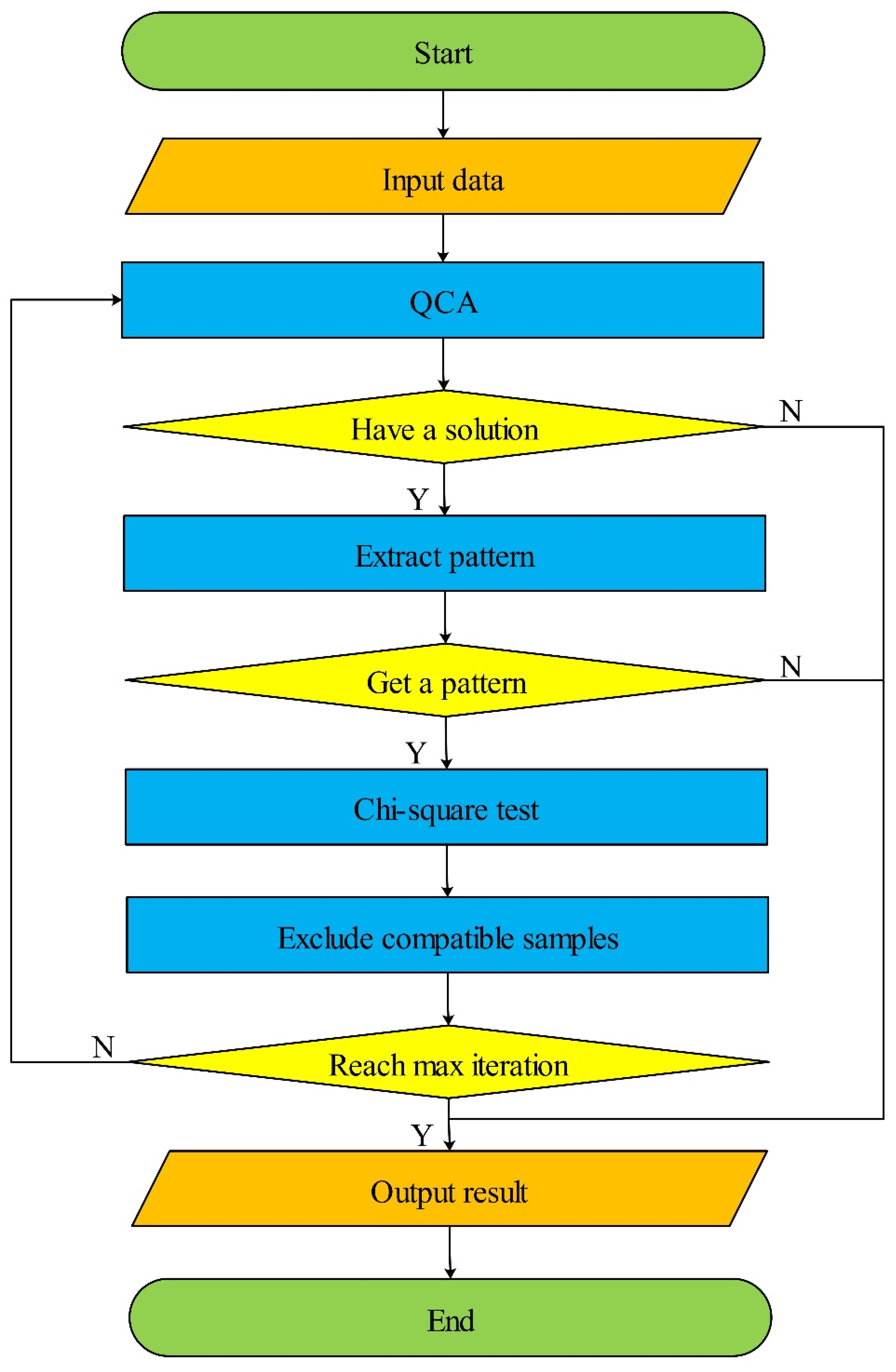
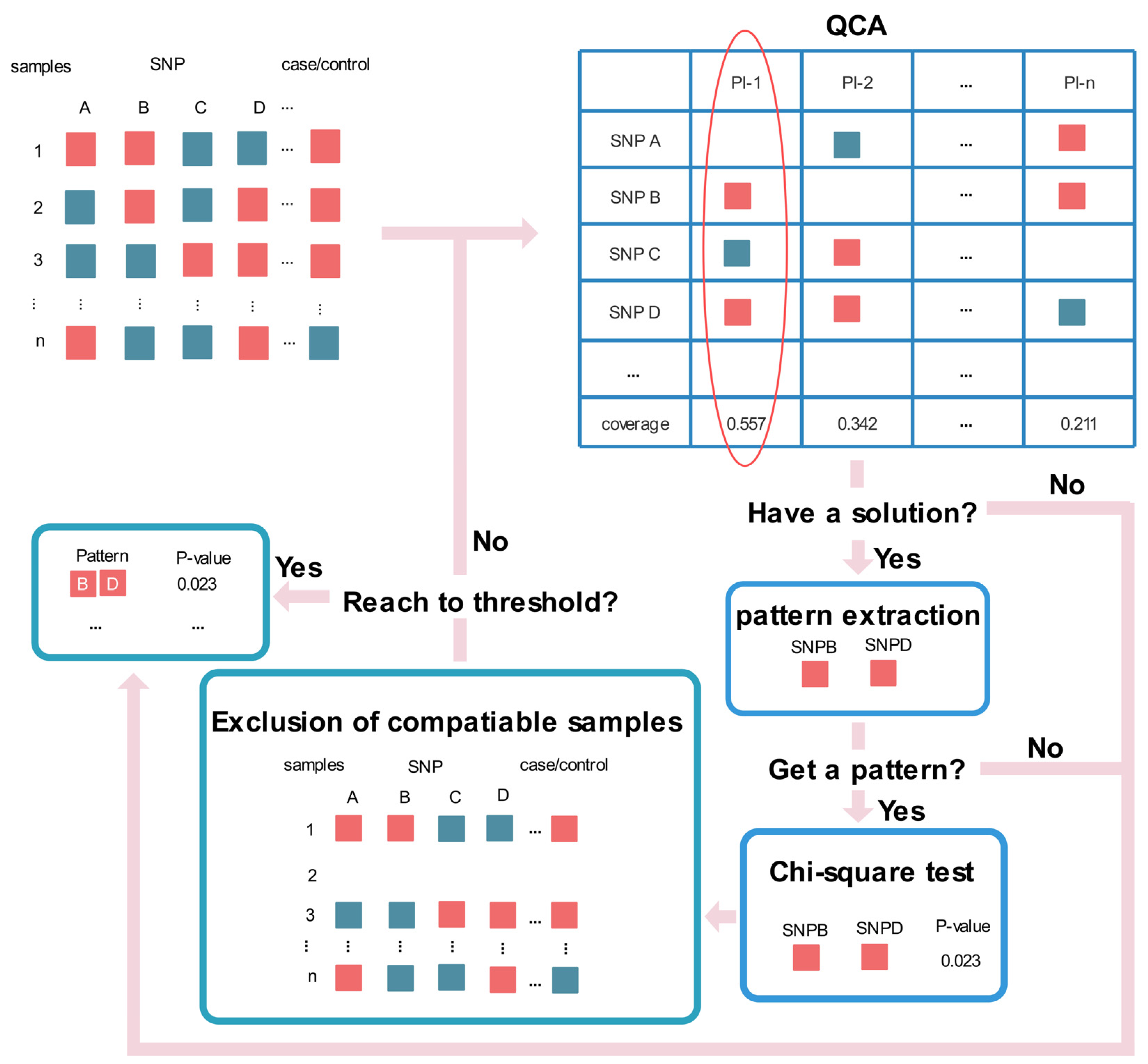
2.1. Iterative Exclusion of Compatible Samples Workflow

In set theory, the definition of a subset is as follows: consider two sets X and Y, if every element in X is also an element in Y, then X is a subset of Y. A subset is a sufficient condition for a superset, and it can be logically deduced that if X, then Y. In real situations, there are very rare complete subset relationships. Therefore, it is necessary to evaluate the extent to which a condition set is sufficient for an outcome set, namely, consistency. Consistency represents the proportion of samples with a particular antecedent or a combination of antecedents with the same outcome. Coverage represents the extent to which the subset covers the target set, which can be used to measure the empirical importance of a particular antecedent or a combination of antecedents and represents the explanatory power of the dataset with respect to the result.
QCA explores how the outcome occurs as a whole by examining the subset relationship of sufficiency between the conditional variables and the outcome variable. In sufficiency analysis, the conditional variable is taken as the subset of the outcome variable, whose consistency is calculated by Equation (1).
Consistency ( X i Y i ) = [ min ( X i , Y i ) ] / ( X i )
The coverage is calculated by Equation (2).
Coverage ( X i Y i ) = [ min ( X i , Y i ) ] / ( Y i )
where Xi denotes the value of the conditional variable and Yi denotes the value of the outcome variable.
The flow chart of IECS is presented in Figure 1. In IECS, the iteration of four steps (QCA, pattern extraction, the chi-square test, and exclusion of compatible samples) is used to analyze the sufficiency relationship between SNPs and complex diseases.
QCA obtains the solution by constructing a truth table according to the dataset and performing Boolean minimization, simplification, and elimination of some conditional variables, and the resultant solution is a combination of multiple prime implicants. If there is no solution, the items obtained in previous rounds of iteration are output, and the IECS workflow is ended.
Pattern extraction selects the prime implicant with the greatest raw coverage in the solution, extracts the conditional variables with “1”, and combines these conditional variables into a pattern. If all the conditional variables in the prime implicant are “0”, the prime implicant with the second greatest raw coverage is selected, and so on. If no pattern can be extracted from all prime implicants in the solution, the items obtained in previous rounds of iteration are output, and the IECS workflow is ended.
The chi-square test is then employed to test whether the pattern is related to the complex disease in the source dataset.
Exclusion of compatible samples is performed to exclude all samples compatible with the pattern and subject the remaining samples to the next round of analysis.
This cycle of processes is repeated until the preset maximum number of iterations is obtained, the results are output, and the IECS workflow is ended.
IECS can work in two modes: the first mode restricts the number of iterations, while the second mode has no limitations on the number of iterations. In the first mode, assume that the number of iterations is set to k. If each round of QCA produces a solution and a pathogenic pattern can be extracted, the program will iteratively run until the preset number of iterations is reached. However, if QCA has no solution or no pathogenic pattern can be extracted in a certain round, the program will end and n pathogenic patterns will be obtained (n < k). On the other hand, in the second mode, the program will run iteratively until the next round of QCA calculation has no solution or no pathogenic pattern can be extracted. It is recommended to initially limit the number of iterations to a smaller value and then decide whether to increase the number of iterations or switch to the second mode after observing the results. This approach helps avoid excessive analysis time in the beginning.
The framework of IECS with data examples is presented in Figure 2. In the first mode, IECS performs the first round of analysis: QCA obtains n prime implicants, among which PI-1 has the greatest coverage (0.557). Therefore, the pathogenic pattern of simultaneous mutations of SNP B and SNP D is extracted from PI-1. The p-value (0.023) for this pathogenic pattern is calculated in the source dataset. Next, samples that are compatible with the pathogenic pattern (such as sample 2, etc.) are excluded. Then, it is checked whether the number of iterations has been reached. If so, the IECS workflow is ended, and all the items are output. If not, IECS continues with a following round of iterations with the remaining samples. During the iterations, if the solution of QCA is empty or the extracted pathogenic pattern is empty, the items obtained in previous rounds of iteration are output, and the IECS workflow is ended.
In the second mode, IECS works until a certain round of QCA solution is empty or the extracted pathogenic pattern is empty.
The pseudocode of IECS is as following Algorithm 1. The code folder is available at https://github.com/happyputi/IECS (accessed on 10 October 2023).
Algorithm 1 IECS
Input: k: threshold of iterations; consistency threshold: threshold of consistency;
U: set of samples.
Output: Solution: The SNP combinations with p-value of chi-square test.
1: Solution ← ∅
2: V ← U
3: W ← U
4: For i = 1 → k do
5: X ← qca(V)
6: If X.length == 1 then
7: Break
8: Else
9: Z ← Extractpattern(X)
10: p ← Chisquaretest(Z, W)
11: V ← Excludesamples(V)
12: Z ← Append(Z, p)
13: Solution ← Append(Solution, Z)
14: End if
15: End for

2.2. Analysis of Necessary Conditions

Analysis of necessary conditions considers complex diseases as the subsets of single SNPs and calculates the consistency and coverage parameters. Then, single SNPs with consistency and coverage greater than the threshold are selected, followed by a chi-square test to screen single SNPs as the necessary conditions (with statistical significance) of complex diseases.

2.3. Performance Measurements

The recognition ability (power) and runtimes of MDR, BOOST, and IECS were compared. Measurement of power was performed with the proportion of the number of datasets identified by the algorithm to that of all datasets [35]. Power is calculated as follows:
Power = N T / N D
where NT denotes the number of identified datasets determined by whether the whole solution has at least one item that is the same as the item in the logical expression of the pathogenic model [46], and ND denotes the total number of datasets, which was set to 1000 in this experiment. Runtime is obtained by calculating the average time that the program runs in each dataset of each dataset group.

2.4. Simulated Data

Suppose the S disease is caused by the simultaneous mutation of SNP-A and SNP-B or SNP-C and SNP-D, and E is added to stand for any other SNP. The configuration table of all logical combinations of the S disease is expressed as A × B × C × D × E × S, and the pathogenic model is recorded as A × B + C × D = S.
Collection I comprises seven dataset groups introduced with 10%, 20%, 30%, 40%, 50%, 60%, and 70% noise, respectively, and each group contains 1000 datasets, with each dataset including 100 samples.
Collection II comprises seven dataset groups respectively containing 200, 400, 600, 800, 1000, 1200, and 1400 samples, and each dataset group includes 1000 datasets introduced with 30% noise.

2.5. Alzheimer’s Disease Data

The etiology of Alzheimer’s disease (a neurodegenerative disorder) remains unknown [47]. The performance of IECS was further tested in a real dataset of Alzheimer’s disease downloaded from the Kaggle website. This dataset encompasses 257 Chinese individuals diagnosed with sporadic Alzheimer’s disease along with 242 control subjects exhibiting normal cognitive function. The average age of the patients at examination was 76.7 years, and the average age of the controls was 80.0 years.

3. Results and Discussion

All calculations were executed on the same computer with the configuration as follows: CPU, Intel(R) Core(TM) i7-8700 CPU @ 3.20 GHz; RAM, 16.0 GB; OS, Windows 10 64 Bit.

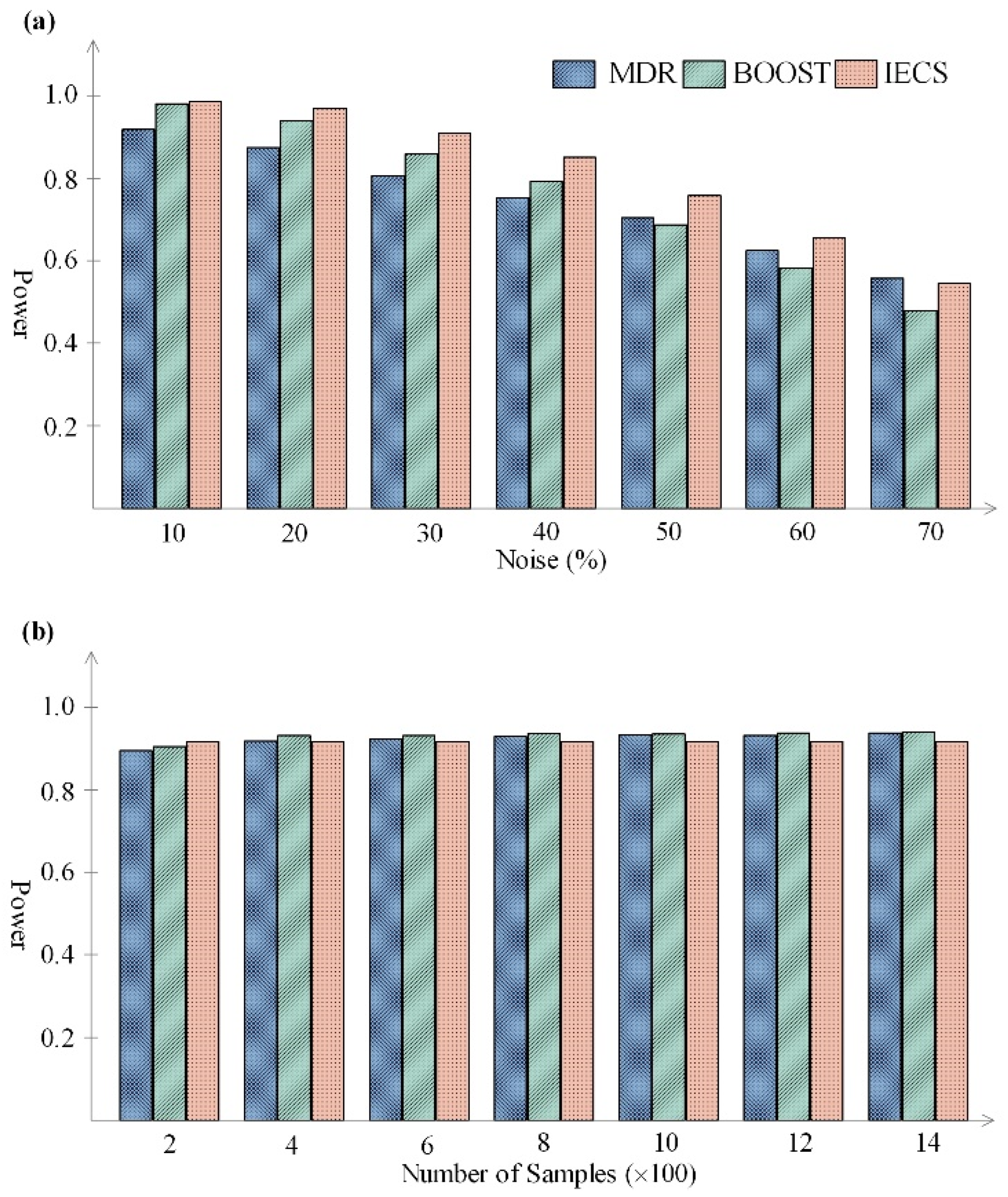
3.1. Simulated Data Experiment

For Collection I, the power levels of IECS, MDR, and BOOST are presented in Figure 3a. The results revealed that when the noise was lower than or equal to 60%, IECS exhibited a greater power compared to both the MDR and BOOST methods; when the noise level reached 70%, the power of IECS was slightly smaller than that of MDR, but greater than that of BOOST. IECS utilizes QCA for calculation and then extracts the pattern for the chi-square test, which can minimize the negative impact caused by noise and then more accurately identify SNP interactions.
Noise showed a great influence on the power: the power of IECS, MDR, and BOOST was close to 1 when the noise was 10% and gradually decreased with increasing noise. A greater noise ratio represents more interfered samples. For MDR, a greater noise ratio means a greater error probability to define different combinations of SNP pairs and accordingly a higher probability of incorrect results in the cross-validation, thereby leading to the smaller power of the algorithm; for BOOST, it means a lower probability that the distribution of the contingency table is consistent with the pathogenic model, so the power is smaller; and for IECS, it means a greater reduction in the consistency and coverage during QCA, which has a greater impact on the identification process and then leads to smaller power.
The runtimes of IECS, MDR, and BOOST for simulated data with different noise ratios are shown in Table 1. In general, BOOST is the fastest, followed by IECS and then MDR. MDR performs the permutation test on generated multiple new datasets by randomly shuffling the outcome of the original samples and then carries out MDR analysis on these new datasets, which is very computationally intensive, resulting in its having the lowest speed among IECS, MDR, and BOOST. BOOST employs an approximate approach to evaluate all pairs of loci by calculating the approximate likelihood ratio in a non-iterative way, which reduces the runtime by simplifying the calculation. With increasing noise ratio, the runtime remains almost constant.
For Collection II, the power levels of IECS, MDR, and BOOST for simulated data with different numbers of samples are presented in Figure 3b. With an increasing number of samples, the power of MDR and BOOST increases slowly, while that of IECS remains almost constant. With more samples, more information about the pathogenic model could be obtained by MDR and BOOST, which would contribute to a greater power. However, in IECS, the QCA calculation engine becomes insensitive to the number of samples beyond a certain amount. When the noise is constant, the number of excluded samples will be adjusted proportionally, and then the extracted pattern is almost unchanged, resulting in the constant power of IECS.
The runtimes of IECS, MDR, and BOOST for simulated data with different numbers of samples are presented in Table 1. With an increasing number of samples, the runtime of MDR and IECS will increase, because more information needs to be calculated for more samples, and therefore more runtime is consumed. BOOST employs an approximate approach to evaluate all pairs of loci by calculating the approximate likelihood ratio in a non-iterative way, which is not sensitive to the number of samples, resulting in an almost constant runtime.
Based on the above results of simulated datasets with a comprehensive comparison of power and runtime, IECS has a stronger recognition ability for pathogenic models with an acceptable runtime.

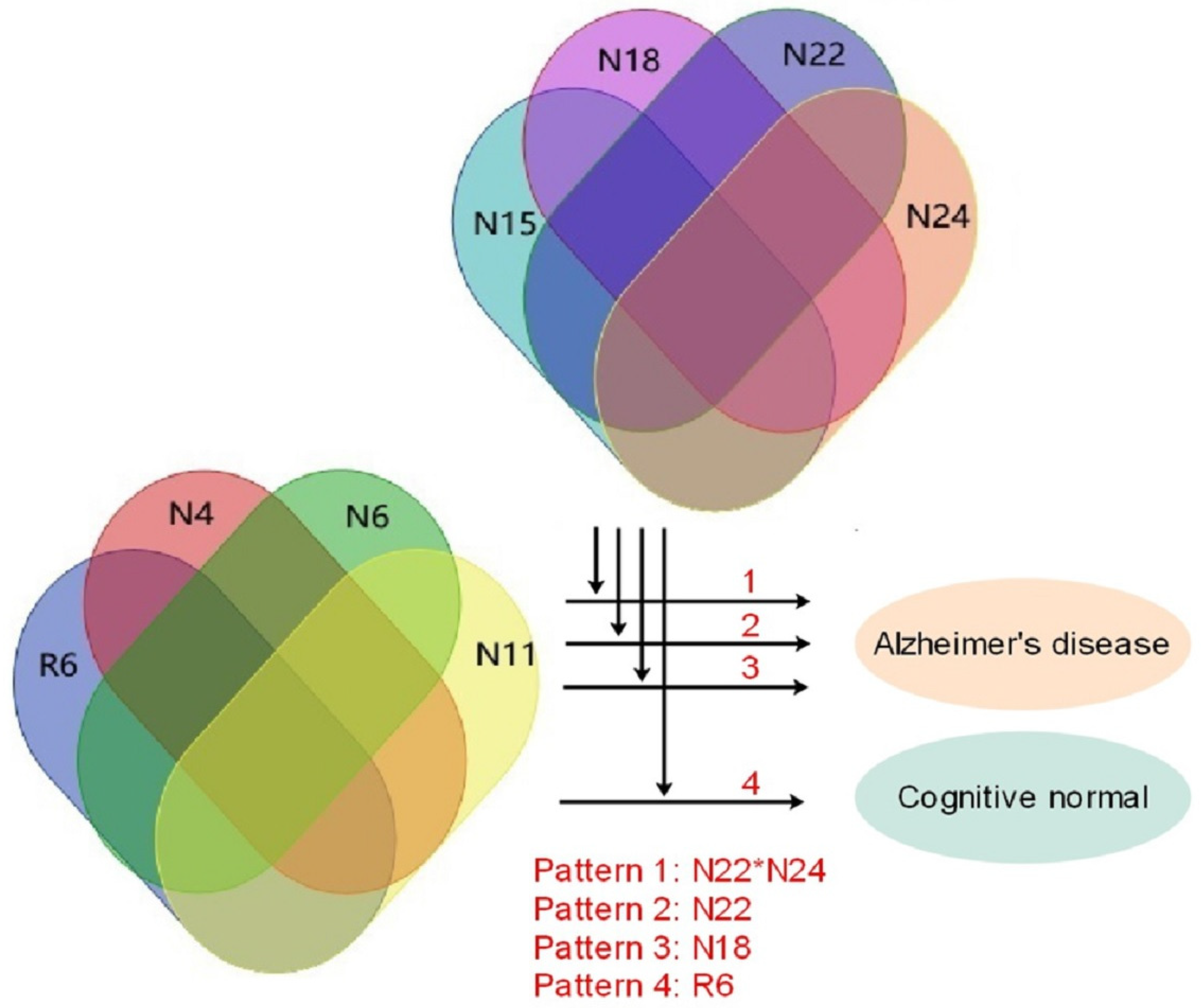
3.2. Alzheimer’s Disease Data Experiment

The dominant model was adopted to code homozygous wild-type alleles as 0 and heterozygous wild-type and mutant alleles or homozygous mutant alleles as 1.
Four iterations were completed in the IECS workflow. The pattern of the simultaneous mutation of SNP (IV S22 + 36 C > A) and SNP (3′UT R159 C > T) was extracted in the first round; the IV S17 − 294 C > T mutation pattern was extracted in the second round; the simultaneous mutation pattern of IV S3 + 106 T >G, IV S10 − 5 C > T, and 3 ’UT R159 C > T was extracted in the third round; and the IV S22 + 36 C > A mutation pattern was extracted in the fourth round. Please refer to Table 2 for the results of the QCA analysis.
The chi-square test was employed to analyze the predictive power of the four patterns in the source dataset, and the p-value of the pattern with simultaneous mutation of IV S3 + 106 T > G, IV S10 − 5 C > T, and 3′UT R159 C > T was 0.909, which was greater than 0.05, and therefore this pattern was excluded from the pathogenic model.
The relationship between SNPs and Alzheimer’s disease was obtained by IECS. If IV S22 + 36 C > A and 3′UT R159 C > T are simultaneously mutated, or IV S17 − 294 C > T or IV S22 + 36 C > A is mutated, the individual might get Alzheimer’s disease.
The Alzheimer’s disease data were also analyzed by MDR and BOOST, and the results and comparisons with those of IECS are shown in Table 3. IECS obtained three significant items with a runtime of 4.496 s. MDR obtained one significant item, namely, the simultaneous mutation of IV S22 + 36 C > A and 3′UT R159 C > T, with a runtime of 42.591 s. BOOST obtained an insignificant item, namely, the simultaneous mutation of IV S10 − 5 C > T and IV S22 + 36 C > A, with a runtime of 0.368 s.
Previous research has demonstrated the interactive association of Alzheimer’s disease with two SNPs, namely, IV S22 + 36 C > A and 3′UT R159 C > T, located within introns [22]. This interaction was determined using the multifactor dimensionality reduction method based on a log-linear model and the multifactor dimensionality reduction algorithm. IV S17 − 294 C > T in introns was associated with an increase in the risk for Alzheimer’s disease, as indicated by the statistical analysis and the haplotype analysis; in addition, IV S22 + 36 C > A in introns was also related to a higher risk of Alzheimer’s disease [48].
Among IECS, MDR, and BOOST for the Alzheimer’s disease dataset, IECS could obtain more results than MDR and BOOST, its runtime is relatively short, and the results are all supported by the literature, demonstrating that IECS can detect multiple SNPs related to complex diseases.
According to the significance of necessary conditions, we took Alzheimer’s disease as the outcome and eight SNPs as the conditional variables to perform the chi-square test. The relation of necessary conditions was expressed as “No A, then no B” logically. A conditional variable is deemed necessary if its consistency exceeds 0.9 and its coverage surpasses 0.5 [49]. There are four conditional variables necessary for Alzheimer’s disease: ∼−204 G > C, ∼C.401 A > G, ∼IV S10 − 5 C > T, and ∼IV S15 + 144 T > A (“∼” denotes no mutation of the SNP). According to the significance of necessary conditional variables, a chi-square test was conducted by taking the disease as the outcome. The results are shown in Table 4. “No mutation of −204 G > C” under Alzheimer’s disease is significant with a p-value of 0.008, suggesting that if the SNP of −204 G > C is mutated, the individual will not get Alzheimer’s disease. The other three conditional variables are not significant. In a previous study, analysis of the transcription factor binding site performed by Consite showed that the mutation at the position of −204 G > C enables it to enhance the expression of neprilysin and reduce the accumulation of A β (amyloid beta) in the brain, which possibly hinders Alzheimer’s disease [48].
The relationships between SNPs and Alzheimer’s disease obtained by IECS and the analysis of necessary conditions are shown in Figure 4. All results are supported by the literature.

4. Conclusions

The IECS workflow with QCA as the calculation engine was proposed and applied to analyze simulated datasets and the real dataset of Alzheimer’s disease, and its performance was compared with that of the BOOST and MDR algorithms. The results revealed that IECS has greater power with relatively less computation cost. IECS has a relatively acceptable runtime and can compute high-dimensional pathogenic patterns with greater power. IECS could be applied to multi-SNP analysis in complex diseases as well as gene–gene and gene–environment interactions to explore the causes of complex diseases. In further research, we would use IECS to analyze more datasets to explore the causes of complex diseases and accelerate the computing speed of IECS.

Author Contributions

J.G.: idea conceptualization, project administration, and funding acquisition. L.Z., W.X. and X.Z.: methodology and validation. W.X.: article writing. All authors have read and agreed to the published version of the manuscript.

Funding

This research was funded by the National Natural Science Foundation of China (no. 21873034), GHFUND A (no. ghfund202302011713), and RFHBUE (no. XJ201906).

Data Availability Statement

Acknowledgments

The authors would like to thank Hongyu Zhang and Jing Gong of Huazhong Agricultural University for insightful discussions.

Conflicts of Interest

The authors declare no conflict of interest.

References

  1. Komar, A.A. SNPs, Silent but Not Invisible. Science 2007, 315, 466–467. [Google Scholar] [CrossRef]
  2. Korte, A.; Farlow, A. The advantages and limitations of trait analysis with GWAS: A review. Plant Methods 2013, 9, 1–9. [Google Scholar] [CrossRef] [PubMed]
  3. The International SNP Map Working Group; Sachidanandam, R.; Weissman, D.; Schmidt, S.C.; Kakol, J.M.; Stein, L.D.; Marth, G.; Sherry, S.; Mullikin, J.C.; Mortimore, B.J.; et al. A map of human genome sequence variation containing 1.42 million single nucleotide polymorphisms. Nature 2001, 409, 928–933. [Google Scholar] [CrossRef]
  4. Wu, X.; Larson, S.R.; Hu, Z.; Palazzo, A.J.; A Jones, T.; Wang, R.R.-C.; Jensen, K.B.; Chatterton, N.J. Molecular genetic linkage maps for allotetraploid Leymus wildryes (Gramineae: Triticeae). Genome 2003, 46, 627–646. [Google Scholar] [CrossRef]
  5. Culverhouse, R.; Suarez, B.K.; Lin, J.; Reich, T. A perspective on epistasis: Limits of models displaying no main effect. Am. J. Hum. Genet. 2002, 70, 461–471. [Google Scholar] [CrossRef] [PubMed]
  6. Huang, Y.-T.; VanderWeele, T.J.; Lin, X. Joint analysis of SNP and gene expression data in genetic association studies of complex diseases. Ann. Appl. Stat. 2014, 8, 352–376. [Google Scholar] [CrossRef] [PubMed]
  7. Momtaz, R.; Ghanem, N.; El-Makky, N.; Ismail, M. Integrated analysis of SNP, CNV and gene expression data in genetic association studies. Clin. Genet. 2017, 93, 557–566. [Google Scholar] [CrossRef]
  8. Khera, A.V.; Chaffin, M.; Aragam, K.G.; Haas, M.E.; Roselli, C.; Choi, S.H.; Natarajan, P.; Lander, E.S.; Lubitz, S.A.; Ellinor, P.T.; et al. Genome-wide polygenic scores for common diseases identify individuals with risk equivalent to monogenic mutations. Nat. Genet. 2018, 50, 1219–1224. [Google Scholar] [CrossRef] [PubMed]
  9. Nolte, I.M.; Van Der Most, P.J.; Alizadeh, B.Z.; De Bakker, P.I.; Boezen, H.M.; Bruinenberg, M.; Franke, L.; Van Der Harst, P.; Navis, G.; Postma, D.S.; et al. Missing heritability: Is the gap closing? An analysis of 32 complex traits in the lifelines cohort study. Eur. J. Hum. Genet. 2017, 25, 877–885. [Google Scholar] [CrossRef] [PubMed]
  10. Román-Ponce, S.-I.; Samoré, A.B.; A Dolezal, M.; Bagnato, A.; Meuwissen, T.H. Estimates of missing heritability for complex traits in Brown Swiss cattle. Genet. Sel. Evol. 2014, 46, 36. [Google Scholar] [CrossRef]
  11. Freidlin, B.; Zheng, G.; Li, Z.; Gastwirth, J.L. Trend Tests for Case-Control Studies of Genetic Markers: Power, Sample Size and Robustness. Hum. Hered. 2002, 53, 146–152. [Google Scholar] [CrossRef] [PubMed]
  12. Song, K.; Elston, R.C. A powerful method of combining measures of association and Hardy-Weinberg disequilibrium for fine-mapping in case-control studies. Stat. Med. 2006, 25, 105–126. [Google Scholar] [CrossRef]
  13. Zheng, G.; Ng, H.K.T. Genetic model selection in two-phase analysis for case-control association studies. Biostatistics 2007, 9, 391–399. [Google Scholar] [CrossRef]
  14. Nelson, M.; Kardia, S.; Ferrell, R.; Sing, C. A Combinatorial Partitioning Method to Identify Multilocus Genotypic Partitions That Predict Quantitative Trait Variation. Genome Res. 2001, 11, 458–470. [Google Scholar] [CrossRef]
  15. Wang, Y.-T.; Sung, P.-Y.; Lin, P.-L.; Yu, Y.-W.; Chung, R.-H. A multi-SNP association test for complex diseases incorporating an optimal P-value threshold algorithm in nuclear families. BMC Genom. 2015, 16, 381. [Google Scholar] [CrossRef]
  16. Cordell, H.J. Detecting gene–gene interactions that underlie human diseases. Nat. Rev. Genet. 2009, 10, 392–404. [Google Scholar] [CrossRef]
  17. Klein, R.J.; Zeiss, C.; Chew, E.Y.; Tsai, J.-Y.; Sackler, R.S.; Haynes, C.; Henning, A.K.; SanGiovanni, J.P.; Mane, S.M.; Mayne, S.T.; et al. Complement Factor H Polymorphism in Age-Related Macular Degeneration. Science 2005, 308, 385–389. [Google Scholar] [CrossRef]
  18. Risch, N.; Merikangas, K. The Future of Genetic Studies of Complex Human Diseases. Science 1996, 273, 1516–1517. [Google Scholar] [CrossRef]
  19. Chatelain, C.; Durand, G.; Thuillier, V.; Augé, F. Performance of epistasis detection methods in semi-simulated GWAS. BMC Bioinform. 2018, 19, 231. [Google Scholar] [CrossRef] [PubMed]
  20. Ritchie, M.D.; Hahn, L.W.; Roodi, N.; Bailey, L.R.; Dupont, W.D.; Parl, F.F.; Moore, J.H. Multifactor-dimensionality reduction reveals high-order interactions among estrogen-metabolism genes in sporadic breast cancer. Am. J. Hum. Genet. 2001, 69, 138–147. [Google Scholar] [CrossRef] [PubMed]
  21. Hahn, L.W.; Ritchie, M.D.; Moore, J.H. Multifactor dimensionality reduction software for detecting gene–gene and gene–environment interactions. Bioinformatics 2003, 19, 376–382. [Google Scholar] [CrossRef] [PubMed]
  22. Lee, S.Y.; Chung, Y.; Elston, R.C.; Kim, Y.; Park, T. Log-linear model-based multifactor dimensionality reduction method to detect gene–gene interactions. Bioinformatics 2007, 23, 2589–2595. [Google Scholar] [CrossRef] [PubMed]
  23. Lou, X.-Y.; Chen, G.-B.; Yan, L.; Ma, J.Z.; Zhu, J.; Elston, R.C.; Li, M.D. A Generalized Combinatorial Approach for Detecting Gene-by-Gene and Gene-by-Environment Interactions with Application to Nicotine Dependence. Am. J. Hum. Genet. 2007, 80, 1125–1137. [Google Scholar] [CrossRef] [PubMed]
  24. Cattaert, T.; Calle, M.L.; Dudek, S.M.; Mahachie John, J.M.; Van Lishout, F.; Urrea, V.; Ritchie, M.D.; Van Steen, K. Model-based multifactor dimensionality reduction for detecting epistasis in case-control data in the presence of noise. Ann. Hum. Genet. 2011, 75, 78–89. [Google Scholar] [CrossRef] [PubMed]
  25. Greene, C.S.; Sinnott-Armstrong, N.A.; Himmelstein, D.S.; Park, J.P.; Jason, H.M.; Brent, T.H. Multifactor dimensionality reduction for graphics processing units enables genome-wide testing of epistasis in sporadicals. Bioinformatics 2010, 26, 694–695. [Google Scholar] [CrossRef]
  26. Gui, J.; Moore, J.H.; Williams, S.M.; Andrews, P.; Hillege, H.L.; Van Der Harst, P.; Navis, G.; Van Gilst, W.H.; Asselbergs, F.W.; Gilbert-Diamond, D. A simple and computationally effient approach to multifactor dimensionality reduction analysis of gene-gene interactions for quantitative traits. PLoS ONE 2013, 8, e66545. [Google Scholar] [CrossRef]
  27. Yang, C.-H.; Lin, Y.-D.; Chuang, L.-Y.; Chen, J.-B.; Chang, H.-W. MDR-ER: Balancing Functions for Adjusting the Ratio in Risk Classes and Classification Errors for Imbalanced Cases and Controls Using Multifactor-Dimensionality Reduction. PLoS ONE 2013, 8, e79387. [Google Scholar] [CrossRef]
  28. Jung, H.-Y.; Leem, S.; Lee, S.; Park, T. A novel fuzzy set based multifactor dimensionality reduction method for detecting gene–gene interaction. Comput. Biol. Chem. 2016, 65, 193–202. [Google Scholar] [CrossRef]
  29. Yu, W.; Lee, S.; Park, T. A unified model based multifactor dimensionality reduction framework for detecting gene–gene interactions. Bioinformatics 2016, 32, i605–i610. [Google Scholar] [CrossRef]
  30. Yang, C.-H.; Chuang, L.-Y.; Lin, Y.-D. CMDR based differential evolution identifies the epistatic interaction in genome-wide association studies. Bioinformatics 2017, 33, 2354–2362. [Google Scholar] [CrossRef]
  31. Yang, C.-H.; Chuang, L.-Y.; Lin, Y.-D. Multiobjective multifactor dimensionality reduction to detect SNP–SNP interactions. Bioinformatics 2018, 34, 2228–2236. [Google Scholar] [CrossRef]
  32. Zhou, X.; Chan, K.C.C. Detecting gene-gene interactions for complex quantitative traits using generalized fuzzy classification. BMC Bioinform. 2018, 19, 329. [Google Scholar] [CrossRef] [PubMed]
  33. Kooperberg, C.L.; LeBlanc, M. Increasing the power of identifying gene × gene interactions in genome-wide association studies. Genet. Epidemiol. 2018, 32, 255–263. [Google Scholar] [CrossRef] [PubMed]
  34. Herold, C.; Steffens, M.; Brockschmidt, F.F.; Baur, M.P.; Becker, T. INTERSNP: Genome-wide interaction analysis guided by a priori information. Bioinformatics 2009, 25, 3275–3281. [Google Scholar] [CrossRef] [PubMed]
  35. Wan, X.; Yang, C.; Yang, Q.; Xue, H.; Fan, X.; Tang, N.L.; Yu, W. BOOST: A Fast Approach to Detecting Gene-Gene Interactions in Genome-wide Case-Control Studies. Am. J. Hum. Genet. 2010, 87, 325–340. [Google Scholar] [CrossRef] [PubMed]
  36. Matsuda, H. Physical nature of higher-order mutual information: Intrinsic correlations and frustration, Physical review E, Statis-tical physics, plasmas, flids, and related interdisciplinary topics. Phys. Rev. E 2000, 62 Pt A, 3096–3102. [Google Scholar] [CrossRef]
  37. Wu, X.; Dong, H.; Luo, L.; Zhu, Y.; Peng, G.; Reveille, J.D.; Xiong, M. A Novel Statistic for Genome-Wide Interaction Analysis. PLoS Genet. 2010, 6, e1001131. [Google Scholar] [CrossRef]
  38. Ueki, M.; Cordell, H.J. Improved Statistics for Genome-Wide Interaction Analysis. PLoS Genet. 2012, 8, e1002625. [Google Scholar] [CrossRef]
  39. Li, J.; Malley, J.D.; Andrew, A.S.; Karagas, M.R.; Moore, J.H. Detecting gene-gene interactions using a permutation-based random forest method. BioData Min. 2016, 9, 14. [Google Scholar] [CrossRef]
  40. Chen, S.H.; Sun, J.; Dimitrov, L.; Turner, A.R.; Adams, T.S.; Meyers, D.A.; Chang, B.L.; Zheng, S.L.; Grönberg, H.; Xu, J.; et al. A support vector machine approach for detecting gene-gene interaction. Genet. Epidemiol. 2008, 32, 152–167. [Google Scholar] [CrossRef]
  41. Ritchie, M.D.; White, B.C.; Parker, J.S.; Hahn, L.W.; Moore, J.H. Optimization of neural network architecture using genetic programming improves detection and modeling of gene-gene interactions in studies of human diseases. BMC Bioinform. 2003, 4, 28. [Google Scholar] [CrossRef]
  42. Onay, V.; Briollais, L.; A Knight, J.; Shi, E.; Wang, Y.; Wells, S.; Li, H.; Rajendram, I.; Andrulis, I.L.; Ozcelik, H. SNP-SNP interactions in breast cancer susceptibility. BMC Cancer 2006, 6, 114. [Google Scholar] [CrossRef] [PubMed]
  43. Raign, C.C. The Comparative Method: Moving beyond Qualitative and Quantitative Strategies, 1st ed.; University of California Press: Oakland, CA, USA, 1987. [Google Scholar]
  44. McAdam, D.; Boudet, H.S.; Davis, J.; Orr, R.J.; Scott, W.R.; Levitt, R.E. “Site Fights”: Explaining Opposition to Pipeline Projects in the Developing World1. Sociol. Forum 2010, 25, 401–427. [Google Scholar] [CrossRef]
  45. Pappas, I.O.; Woodside, A.G. Fuzzy-set Qualitative Comparative Analysis (fsQCA): Guidelines for research practice in Information Systems and marketing. Int. J. Inf. Manag. 2021, 58, 102310. [Google Scholar] [CrossRef]
  46. Baumgartner, M.; Ambühl, M. Causal modeling with multi-value and fuzzy-set Coincidence Analysis. Politi- Sci. Res. Methods 2018, 8, 526–542. [Google Scholar] [CrossRef]
  47. Kelly, J.; Moyeed, R.; Carroll, C.; Luo, S.; Li, X. Genetic networks in Parkinson’s and Alzheimer’s disease. Aging 2020, 12, 5221–5243. [Google Scholar] [CrossRef]
  48. Shi, J.; Zhang, S.; Tang, M.; Ma, C.; Zhao, J.; Li, T.; Liu, X.; Sun, Y.; Guo, Y.; Han, H.; et al. Mutation screening and association study of the neprilysin gene in sporadic Alzheimer’s disease in Chinese persons. J. Gerontol. Ser. A Biol. Sci. Med. Sci. 2005, 60, 301–306. [Google Scholar] [CrossRef]
  49. Hossain, M.A.; Quaddus, M.; Warren, M.; Akter, S.; Pappas, I. Are you a cyberbully on social media? exploring the personality traits using a fuzzy-set confiurational approach. Int. J. Inf. Manag. 2022, 66, 102537. [Google Scholar] [CrossRef]
Figure 1. Flow chart of IECS workflow. IECS utilizes the iteration of four steps (QCA, pattern extraction, the chi-square test, and exclusion of compatible samples) to analyze the relationship between SNPs and complex diseases.
Algorithms 16 00480 g001
Figure 2. Framework of IECS with data examples. For the data examples, the row name is the sample ID; each column indicates one SNP, except the last column, which indicates whether there is a disease. For conditions, red squares indicate the mutation of the SNP, and green squares indicate no mutation of the SNP. For the result, red squares indicate the disease, green squares indicate no disease. In the first mode, IECS performs the first round of analysis, and QCA obtains n prime implicants, among which PI-1 has the greatest coverage (0.557). Therefore, the pathogenic pattern of simultaneous mutations of SNP B and SNP D is extracted from PI-1. The p-value (0.023) for this pathogenic pattern is calculated in the source dataset. Next, samples that are compatible with the pathogenic pattern (such as sample 2, etc.) are excluded. This cycle of processes is repeated until the preset maximum number of iterations is obtained, the results are output, and the IECS workflow is ended. During the iterations, if the solution of QCA is empty or the extracted pathogenic pattern is empty, the items obtained in previous rounds of iteration are output, and the IECS workflow is ended.
Algorithms 16 00480 g002
Figure 3. (a) The power levels of IECS, MDR, and BOOST for simulated data with different noise levels. When the noise was less than or equal to 60%, the power of IECS was greatest; when the noise was 70%, the power of IECS was slightly less than MDR, but greater than BOOST. (b) The power levels of the three algorithms with different numbers of samples. With the increase in the number of samples, the power of MDR and BOOST increase slowly and IECS remains constant; the more samples, the more information about the pathogenic model obtained by the MDR and BOOST algorithms and the greater the power. However, in IECS, the QCA calculation engine becomes insensitive to the number of samples beyond a certain amount.
Algorithms 16 00480 g003
Figure 4. Relationships between SNPs and Alzheimer’s disease obtained by IECS and analysis of necessary conditions. R6 indicates −204 G > C, N4 indicates IVS3 + 106 T > G, N6 indicates C. 401 A > G, N11 indicates I V S10 − 5 C > T, N15 indicates I V S15 + 144 T > A, N18 indicates I V S17 − 294 C > T, N22 indicates I V S22 + 36 C > A, N24 indicates 3′U T R159 C > T and asterisk “*” indicates simultaneous mutation. Simultaneous mutation of I V S22 + 36 C > A and 3′U T R159 C > T, I V S22 + 36 C > A mutation, and I V S17 − 294 C > T mutation cause Alzheimer’s disease; −204 G > C mutation prevents Alzheimer’s disease.
Algorithms 16 00480 g004
Table 1. Runtimes of IECS, MDR, and BOOST for simulated data with different noise percentages and numbers of samples.
Noise (%)Runtime (Seconds)SamplesRuntime (Seconds)
MDRBOOSTIECSMDRBOOSTIECS
1014.2580.0560.96220013.7830.0560.953
2014.2410.0561.03440017.2430.0591.013
3014.2380.0561.06960020.6580.0631.070
4014.2210.0561.04080024.1590.0741.151
5014.1040.0560.969100026.8100.0681.162
6012.3930.0560.783120030.2030.0711.229
7011.9900.0580.651140033.5740.0751.288
Table 2. QCA results for Alzheimer’s disease data of four iterations.
ConfigurationRound 1Round 2Round 3Round 4
−204 G > C
IVS3 + 106 T > G
c.401 A > G
IVS10-5 C > T
IVS15 + 144 T > A
IVS17-294 C > T
IVS22 + 36 C > A
3′UTR159 C > T
Raw coverage9.73%2.71%1.96%1.51%
Consistency1111
Black circles “●” indicate mutation, while white circles “○” indicate no mutation; the blank spaces indicate “don’t care”; four iterations are completed in the IECS workflow.
Table 3. Comparison of IECS, MDR, and BOOST for Alzheimer’s disease data.
MethodResultp-ValueRuntime
IECSIVS22 + 36 C > A * 3′UTR159 C > T0.0074..496 s
IVS17-294 C > T0.026
IVS22 + 36 C > A0.002
MDRIVS22 + 36 C > A * 3′UTR159 C > T042.591 s
BOOSTIVS10-5 C > T * IVS22 + 36 C > A0.1530.368 s
Asterisks “*” indicate simultaneous mutation.
Table 4. Results of analysis of necessary conditions for Alzheimer’s disease data.
ConditionConsistencyCoveragep-Value
~−204 G > C0.9690.5300.008
~c.401 A > G0.9610.5100.130
~IVS10-5 C > T0.9110.5180.711
~IVS15 + 144 T > A0.9260.5280.082
Tildes “~” indicate no mutation of the SNP.
Disclaimer/Publisher’s Note: The statements, opinions and data contained in all publications are solely those of the individual author(s) and contributor(s) and not of MDPI and/or the editor(s). MDPI and/or the editor(s) disclaim responsibility for any injury to people or property resulting from any ideas, methods, instructions or products referred to in the content.

