Problem-Driven Scenario Generation for Stochastic Programming Problems: A Survey

Abstract

Stochastic Programming is a powerful framework that addresses decision-making under uncertainties, which is a frequent occurrence in real-world problems. To effectively solve Stochastic Programming problems, scenario generation is one of the common practices that organizes realizations of stochastic processes with finite discrete distributions, which enables the use of mathematical programming models of the original problem. The quality of solutions is significantly influenced by the scenarios employed, necessitating a delicate balance between incorporating informative scenarios and preventing overfitting. Distributions-based scenario generation methodologies have been extensively studied over time, while a relatively recent concept of problem-driven scenario generation has emerged, aiming to incorporate the underlying problem’s structure during the scenario generation process. This survey explores recent literature on problem-driven scenario generation algorithms and methodologies. The investigation aims to identify circumstances under which this approach is effective and efficient. The work provides a comprehensive categorization of existing literature, supplemented by illustrative examples. Additionally, the survey examines potential applications and discusses avenues for its integration with machine learning technologies. By shedding light on the effectiveness of problem-driven scenario generation and its potential for synergistic integration with machine learning, this survey contributes to enhanced decision-making strategies in the context of uncertainties.

1. Introduction

Stochastic Programming [1] is a framework for stochastic optimization problems involving decision-making under uncertainties. The incorporation of uncertainties into the models of the optimization problems makes the problem more realistic, but meanwhile, more difficult to solve. To address this challenge, Robust Optimization (RO) [2] is commonly employed when the parameters have known bounds, while Stochastic Programming (SP) is used under the assumption that the distributions of the random variables are either known or can be inferred from data. Consequently, RO aims to identify feasible solutions within predetermined bounds, while SP endeavors to identify optimal solutions that are expected to be feasible for all possible data instances, called scenarios.

Scenario generation is an algorithmic strategy to organize the realizations of the stochastic process with finite discrete distribution, commonly in a tree structure. In such a way, the SP problem can be solved with different decomposition and approximation techniques [3,4]. The quality of the solutions naturally depends on the scenarios used. The solutions are more reliable when more scenarios are considered, while the problem is more difficult to solve. Due to this limitation, it is critical to find the balance to include in the scenario-tree the most informative scenarios that avoid over-fitting and ensure the reliability of the solution. Failure to account for the variability of the stochastic process could lead to sub-optimal solutions. By employing suitably generated scenarios, the initial problem can be effectively solved by using decomposition and approximation techniques, such as Benders Decomposition [5], a widely used technique in SP and RO that divides the original problem into a master problem and a sub-problem, enabling the exchange of information between them to update variable values and constraints. Both problems are solved iteratively until convergence, allowing the resolution of large problems with certain structures.

Various methodologies for scenario-tree generation have been proposed over the years. Classic methodologies are mainly distribution-oriented, which involves fitting statistical models to approximate the probability distribution of the stochastic parameters and then apply sampling techniques based on these distribution. A survey and review of such methodologies can be found in [6,7]. Due to advances in computing power and the evolution of machine learning, research conducted in the field is also beyond the replication of statistical characteristics of the stochastic process. In recent years, a concept of problem-driven scenario generation has been proposed and studied. Under this circumstance, we conduct a survey on recent literature on problem-driven scenario generation methodologies that takes into account the structure of the underlying problem in the scenario generation process. The objective of this investigation is to ascertain the circumstances under which this approach shows effectiveness and/or efficiency. Additionally, we explore possible avenues for the integration of such an approach with machine learning technologies.

The remainder of the paper is organized as follows. In Section 2, we provide the formulations of the Stochastic Programming problems and solving techniques, leading to the concept of quality evaluation of a scenario-tree in Section 3. Difference between distribution-oriented and problem-oriented scenario generation is explained in Section 4, which includes categorization of the existing literature on problem-driven scenario generation across various dimensions and accompanied by the presentation of example problems. In Section 5, potential applications of the problem-driven scenario generation approach are discussed. The conclusions are finally drawn in Section 6.

2. Problem Definition

2.1. A Two-Stage Stochastic Programming Problem

Suppose that a decision $x\in {\mathbb{R}}^n$ has be taken based on the information available at the time, while a stochastic process $\xi \in {\mathbb{R}}^d$ exists and its value can only be observed in the future. A general two-stage SP problem can be represented as follows [1]:

$$\underset{x\in X}{min}f\left(x\right)+{\mathbb{E}}_{\xi }\left[Q(x,\xi )\right],$$

(1)

where $f\left(x\right)$ is a continuous function representing the first-stage costs, X is the feasibility set for x defined by constraints and $Q(x,\xi )$ is the optimal value of the second-stage problem, also known as the recourse problem:

$$Q(x,\xi )=\underset{y}{min}\left\{q(y,\xi )\right|U\left(\xi \right)x+W\left(\xi \right)y\le h\left(\xi \right)\},$$

(2)

where $y\in {\mathbb{R}}^m$ is the second-stage decision vector, $q(y,\xi )$ is the cost of the recourse action in which $W\left(\xi \right)y$ compensates for a possible inconsistency of the system $U\left(\xi \right)x\le h\left(\xi \right)$ when the uncertain data $\xi$ are revealed.

The two-stage SP problem assumes that the stochastic process is realized only after the first-stage decisions have been made. The objective is to find an optimal decision that fulfills the constraints while taking into account possible realizations of the uncertainties in the coming future. For example, in a simple investment planning problem, a company has a limited budget and faces risks in returns for several projects. In the first stage, it decides which projects to invest in based on the expected returns. Further adjustment can be made to maximize the profit (or minimize the cost) in the second stage, after the actual returns are revealed.

In real-world applications, the problems usually involve a series of decisions that respond to evolving outcomes over time. To account for this, the multi-stage Stochastic Programming model that generalizes two-stage SP problems has been proposed to include sequential uncertainty realizations.

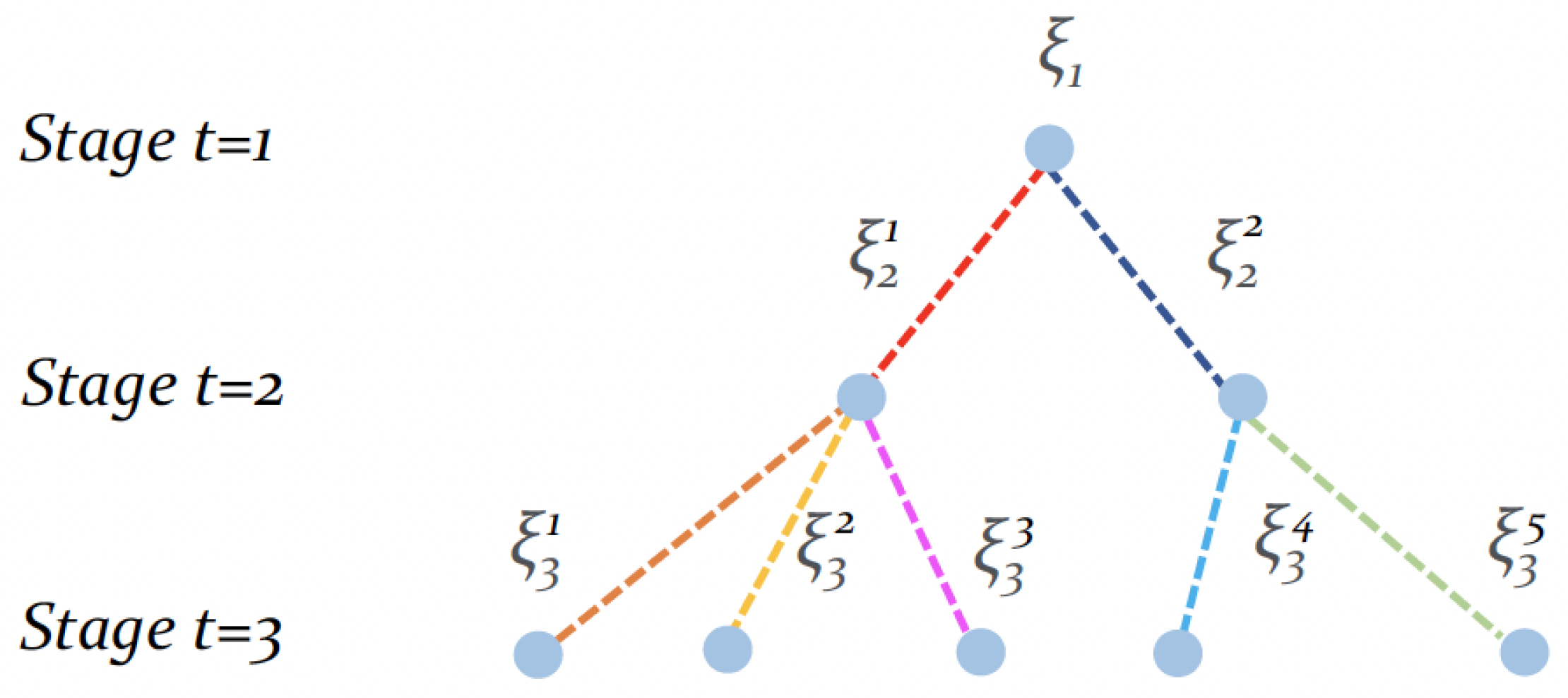
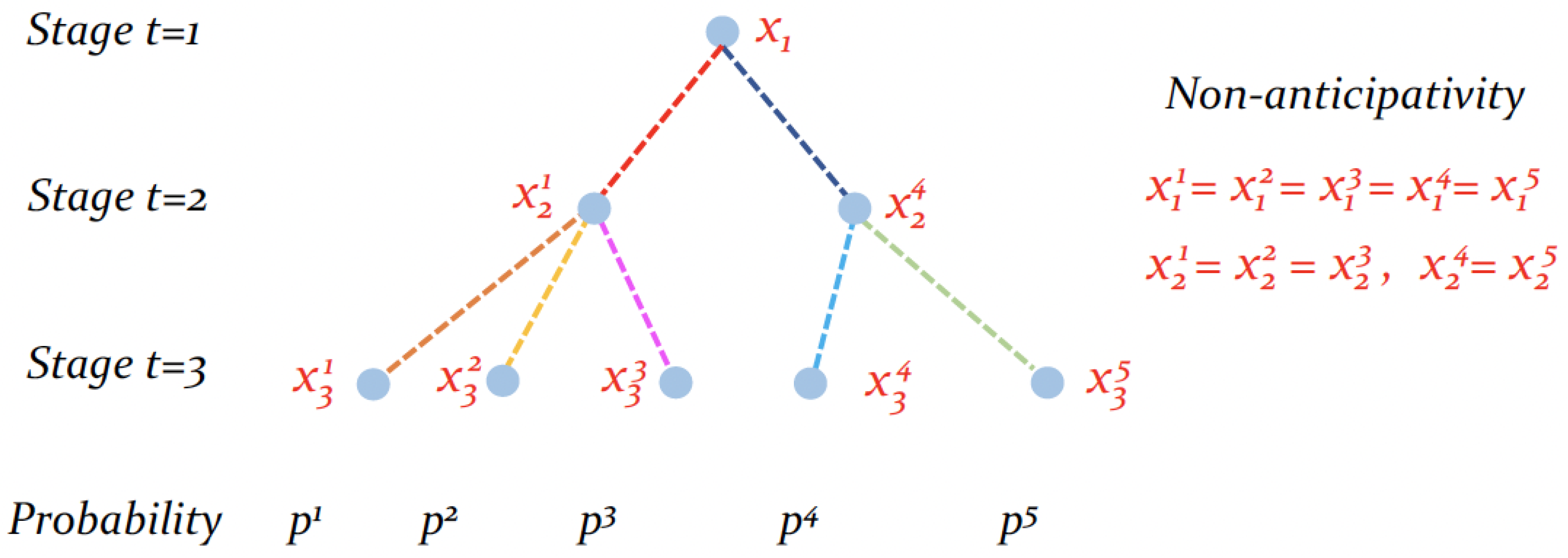
2.2. A Multi-Stage Stochastic Programming Problem

Let us consider a set of time stages $t=\{1,\dots ,T\}$ and a random vector $\xi \in {\mathbb{R}}^d$ that represents the uncertain parameters of a problem, whose value is revealed gradually over time t. The realization of the random vector is denoted as ${\left\{{\xi }_t\right\}}_{t=1}^T$. In practice, ${\xi }_1$ is a fixed value and ${\xi }_t$ is the observation value of the stochastic process following a specified probability distribution when $t>1$. At each stage, a decision $x_t\in {\mathbb{R}}^n$ must be taken with knowledge available up to stage t, and the future realizations ${\xi }_{t+1},\dots ,{\xi }_T$ are still to be observed. This concept is known as non-anticipativity. With these notations, a generic multi-stage Stochastic Programming problem that aims at maximizing the profit can be represented as follows:

$$\underset{x_1,\dots ,x_T}{max}{f}_1\left(x_1\right)+{\mathbb{E}}_{\xi }\left[\sum _{t=2}^T{f}_t(x_t,{\xi }_t)\right]$$

(3)

s.t.

$$x_1\in X_1$$

(4)

$$x_t\in X_t(x_{t-1},{\xi }_t),\forall t\in \{2,\dots ,T\},$$

(5)

where $f_t$ is a continuous function, $X_t\subseteq {\mathbb{R}}^n$ is the feasibility set for the decision $x_t$ that depends on the decision $x_{t-1}$ at the previous stage and the observation ${\xi }_t$.

Different from the formulation represented by Equations (1) and (2), which exclusively involve two decisions, the initial decision x and the recourse decision y, the multi-stage problem model (3)–(5) accommodates sequential decisions $x_t$ over multiple time periods. This introduces greater complexity and computational demands. In multi-stage optimization problems, the optimal decision is often hard to compute, especially when the underlying uncertain parameters are modeled by continuous random vectors. Therefore, a variety of approximation methods have been developed in which the stochastic process is approximated over a finite number of scenarios, commonly organized in a tree structure, i.e., a scenario-tree (see Figure 1). In the following section, we will provide a comprehensive discussion concerning the application of a scenario-tree and the implementation of solving techniques in SP problems.

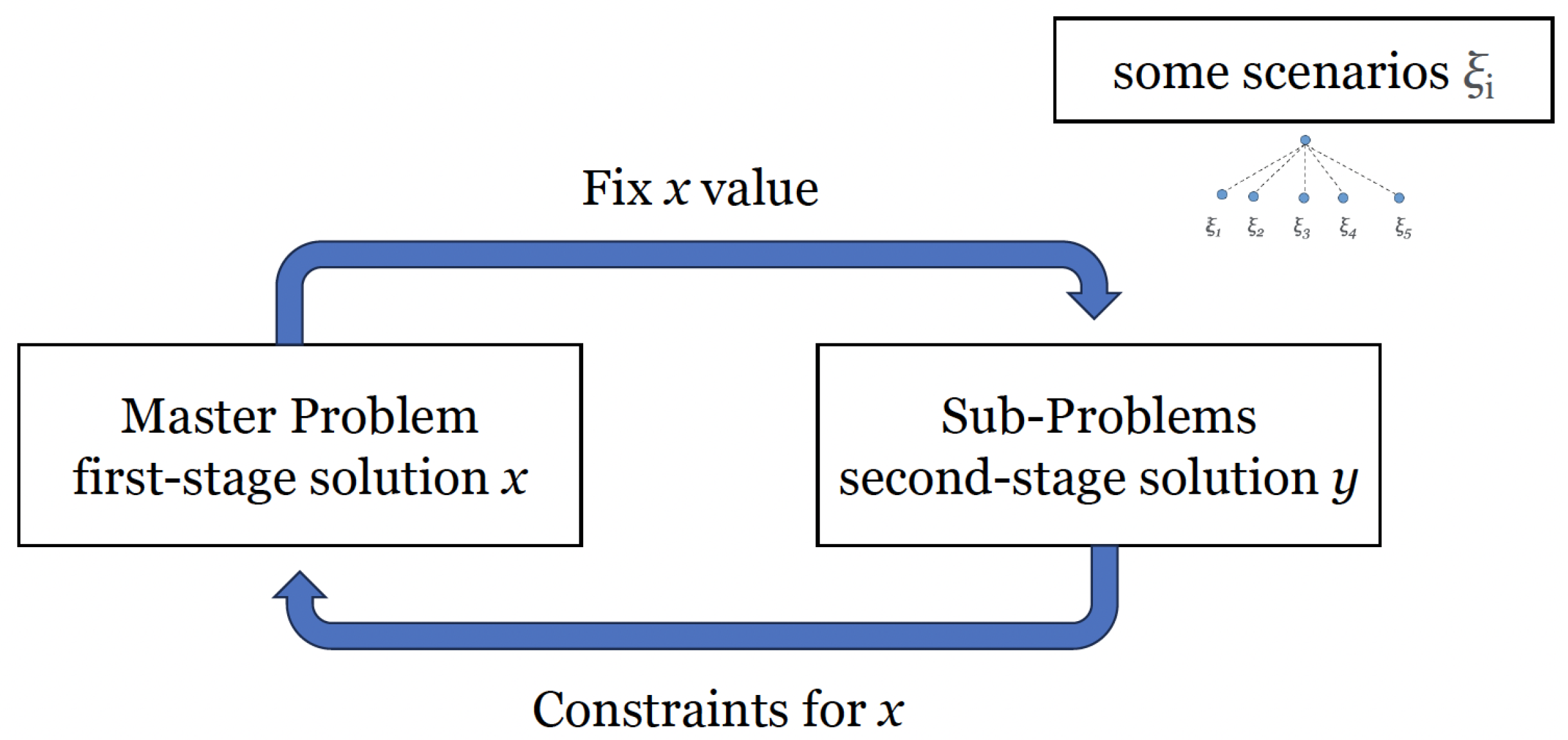
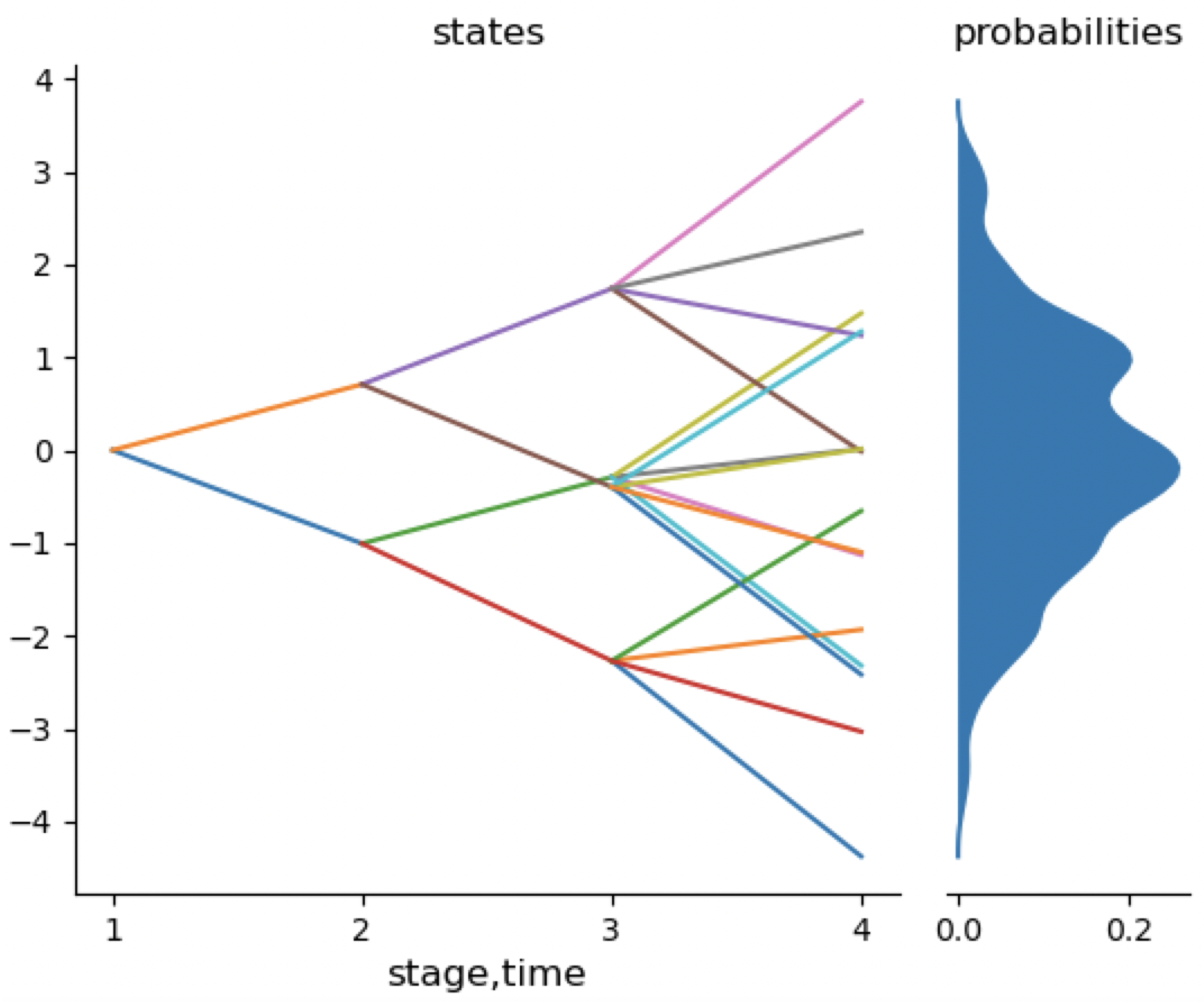
2.3. Scenario-Tree and Solving Techniques

In a scenario-tree, each scenario is depicted as a distinct path originating from the tree’s root and terminating at one of its leaves. The nodes traversing along each path correspond to the specific values taken by random parameters in the model. When continuous variables are involved, a finite and tractable scenario-tree can be constructed by using sampling techniques. A common approach is the Monte Carlo sampling [8,9,10]. The sample average approximation (SAA) for the objective function $f\left(x\right)$ can be simply formulated as follows:

$$\frac{1}{n}\sum _{i=1}^{n}f(x,{\xi }_i).$$

(6)

There are other examples such as quasi-Monte Carlo methods [11], Hidden Markov Models [12], Optimal Quantization [13], Moment-Matching [14], etc. We refrain from providing a detailed discussion of these methodologies in this work. By employing a scenario-tree, the SP problems can be solved with mathematical programming models. Among these approaches, one direct approach is to solve the corresponding Deterministic Equivalent problem.

As an illustrative example, we consider a multi-stage SP problem under the assumption that both the constraints and the objective function are linear. Consequently, the multi-stage SP problem defined by (3)–(5) can be reformulated as follows:

$$\underset{x_1,\dots ,x_T}{max}{c}_1{x}_1+{\mathbb{E}}_{\xi }\left[\sum _{t=2}^T{c}_t\left({\xi }_t\right)x_t\right]$$

(7)

s.t.

$$A_1{x}_1={\mu }_1$$

(8)

$$B_t\left({\xi }_t\right)x_{t-1}+A_t\left({\xi }_t\right)x_t={\mu }_t\left({\xi }_t\right),\forall t\in \{2,\dots ,T\}$$

(9)

$$x_t\ge 0,\forall t\in \{1,\dots ,T\}.$$

(10)

By employing a scenario-tree, the stochastic process ${\xi }_t$ is sampled by a set of S distinct scenarios. In each scenario s, the function $c_t\left({\xi }_t\right)$ in (7) takes a fixed value for each stage t. We denote the decision variable at each stage in each scenario as $x_t^s$ and it may assume varying values across different scenarios. The Deterministic Equivalent problem for the problem (7)–(10) is then defined as follows:

$$\underset{x_1,x_2^s,\dots ,x_T^s}{max}{c}_1{x}_1+\sum _{s=1}^S{p}^s[c_{s,2}{x}_2^s+\cdots +c_{s,T}{x}_T^s]$$

(11)

s.t.

$$A_1{x}_1={\mu }_1$$

(12)

$$B_{s,t}{x}_{t-1}^s+A_{s,t}{x}_t^s={\mu }_{s,t},\forall t\in \{2,\dots ,T\},\forall s\in \{1,\dots ,S\}$$

(13)

$$x_t^s\ge 0,\forall t\in \{1,\dots ,T\},\forall s\in \{1,\dots ,S\}$$

(14)

$$x_t^j=x_t^k,\mathrm{if}{\xi }_t^j={\xi }_t^k,$$

(15)

where $p^s$ is the probability associated with scenario s. Equations (12)–(14) are the constraints defining the feasibility set for the decisions $x_t^s$ in each scenario s. Constraint (15) represents the non-anticipativity conditions, which indicates every pair of scenarios j and k indistinguishable up to stage t shares the same decision at stage t (see Figure 2). In particular, the first stage solution $x_1^s$ assumes equal values in all scenarios, i.e., $x_1^s=x_1$.

Through the resolution of the Deterministic Equivalent problem (11)–(15) with each scenario s, it becomes feasible to derive an approximate solution for the original Stochastic Programming problem (7)–(10). Nevertheless, it is essential to note that in this approach, the computational time grows exponentially as the number of scenarios increases. Consequently, solving the Deterministic Equivalent problem becomes infeasible when dealing with a substantial number of scenarios. Given this challenge, decomposition algorithms, such as Lagrangian decomposition [15,16] and Benders decomposition [5] present more effective alternatives as solving techniques. An illustrative example of solving the two-stage SP problem (see Section 2.1) with Benders decomposition is shown in Figure 3. The original problem is decomposed into two parts: A master problem that searches for the optimal values of the first-stage decision variables x, and sub-problems that, given a fixed value of x obtained from the master problem, solve for the optimal recourse decisions y with different scenarios ${\xi }_i$. In each iteration, the master problem offers a fixed x value to the sub-problems and the sub-problems generate feasibility and optimality cuts for x, which are constraints added to the master problem to be solved with. The master problem and sub-problems are iteratively solved until convergence, leading to the optimal solution for the original SP problem. In multi-stage SP problems, the application of Benders decomposition transforms into a nested Benders decomposition. We suggest the work of [17] for more comprehensive details.

Regarding implementations of the solving techniques, the SP problems can be represented through the utilization of modeling frameworks such as Pyomo [18,19] in Python [20], JuMP [21] in Julia [22], SAMPL [23] based on AMPL [24], and GAMS [25]. The solving of the represented models can be accomplished by using solvers such as CPLEX [26] and Gurobi [27]. A demonstration of the implementation of Benders decomposition through the utilization of JuMP and the Julia programming language is available in [28]. Additionally, a broader framework employing JuMP has been extensively discussed in [29].

Irrespective of the specific solving techniques employed, in SP problems, the quality of the obtained solutions relies significantly on the scenario-tree employed. For the aforementioned solving techniques, the scenario-tree always plays an important role as it must cover a wide array of possibilities, from the best-case to worst-case scenarios, while effectively capturing the most probable outcomes of the problem. Accurately describing the problem in such a manner is expected to result in a more precise or robust solution from the model. In the following section, the quality evaluation of a scenario-tree and its correlation with the quality of the obtained solution is thoroughly discussed.

3. Quality Evaluation of a Scenario-Tree and a Solution

Due to computational efficiency considerations, scenario-trees often contain a finite number of scenarios, which can lead to the solution providing decisions exclusively for a subset of random parameter values. This raises two issues that must be considered: firstly, it necessitates the development of suitable evaluation methodologies for selecting the most representative scenarios to be included in the scenario-tree. Secondly, it initiates the exploration of generalization techniques that are capable of extending the results obtained with a specific scenario-tree to cover all possible scenarios. In this section, we will examine each of these issues in a detailed and systematic manner.

3.1. In-Sample and Out-of-Sample Performance

Regarding the evaluation of performance in optimization problems, computing time (or tractability in the case of computationally challenging problems) and the quality of a solution serve as typical performance metrics. The evaluation of these performance aspects for a solution derived from a specified scenario-tree using the same scenario-tree is referred to as “in-sample performance” evaluation. To derive an accurate objective function value, it is common practice to perform an out-of-sample evaluation, which evaluates the solution’s performance on scenarios outside the scenario-tree. This evaluation is crucial in validating models across different fields. As an illustration, the scenario-tree can be conceptualized as a training set in machine learning, wherein the model is trained and learns from the provided data. Correspondingly, the out-of-sample evaluation serves as a validation set, where the model’s performance is assessed on unseen data to evaluate its generalization capabilities.

In SP problems, a solution is obtained by using a specific scenario-tree. The solution is expected to be feasible and optimal for all cases considered, while keeping a reasonable computing time. Consequently, the size of the scenario-tree is constrained, which can lead to disparities between the in-sample and out-of-sample performance. In consideration of this premise, the work presented in [30] introduces a scenario generation process by minimizing a loss function that measures the discrepancy between out-of-sample and in-sample performance of the solutions. The criterion for a desirable scenario-tree $\mathcal{T}$ is also established as follows: Given a set of solutions to be evaluated both out-of-sample and in-sample with respect to the actual distribution $\xi$, in a good scenario-tree $\mathcal{T}$:

• The ranking of the solutions is preserved: if solution $x_1$ outperforms $x_2$ when evaluated out-of-sample, it should be highly probable that $x_1$ will also outperform $x_2$ when evaluated in-sample.
• Overconfident outliers should be excluded. An outlier is defined as the inconsistency between the out-of-sample $f(x,\xi )$ and in-sample values $f(x,\mathcal{T})$. For example, for a solution $x_1$ better than $x_2$ in a maximizing problem:

  –

  If $f(x_1,\xi )>f(x_2,\xi )$, $f(x_1,\mathcal{T})<f(x_2,\mathcal{T})$ while $f(x_1,\xi )\approx f(x_2,\xi )$, it is an acceptable outlier.

  –

  If $f(x_1,\xi )<f(x_2,\xi )$, $f(x_1,\mathcal{T})>f(x_2,\mathcal{T})$, it is a non-acceptable outlier.

• The in-sample values approximate well the out-of-sample values: $f(x,\xi )\approx f(x,\mathcal{T})$.

The criterion shows that a fundamental metric for assessing the quality of scenario-trees is their capacity to effectively preserve the quality of a solution. The discussion highlights that, when assessing the quality of scenario-trees, the out-of-sample performance carries greater importance than the in-sample performance, particularly when inconsistencies arise between the two. This leads to the stability arguments that address the robustness of the tree. A survey on stability-based approaches for scenario generation can be found in [31]. Several classical methodologies in Stochastic Programming have been discussed, together with a comprehensive review on optimal scenario reduction methods and techniques for generating scenario-trees.

Regarding the stability arguments and robustness of scenario-trees, a natural consideration arises that a scenario-tree is good when a substantial number of scenarios are incorporated. This is, however, impractical due to computational efficiency constraints. Therefore, another focus of attention centers on determining the minimum number of scenarios required. Two simple approaches exist in this regard, offering insights into identifying an optimal scenario-tree size that strikes a balance between computational efficiency and the desired level of stability:

• Initiating with an empty scenario-tree, scenarios are gradually added until stability is achieved. This iterative process continues until the desired level of stability is attained.
• Beginning with a large stable scenario-tree containing numerous scenarios, scenarios are successively removed to observe the loss of stability during the reduction process.

Under these circumstances, the construction of an effective scenario tree necessitates an understanding of the specific scenarios that create variations in the solutions. Sensitivity analysis [32] emerges as another widely used approach for the quality evaluation of scenario-trees. It is a process of investigating the impact of variations in the model’s input parameters on the resulting output. In the work [33], a concrete theoretical foundation for assessing the optimal-value error is proposed, which denotes the difference between the optimal value of the original SP problem and that of the approximated problem generated using different scenario-trees. The study highlights that sub-optimal discretization at a node in the scenario-tree generation process contributes to the optimal-value error, and suggests that suitable scenario-trees can be designed to numerically integrate specific classes of functions determined by the problem’s structure. The findings confirm the practicality of the problem-driven scenario generation approach.

In addition to assessing the quality of scenario-trees in terms of stability and robustness, an auxiliary objective is to find the balance between the quality of the tree and the speed of computation. This leads to the scenario reduction [34], wherein the goal is to identify a smaller subset of scenarios to reduce numerical complexity while maintaining a satisfactory level of accuracy.

3.2. Generalization of a Solution Obtained from a Scenario-Tree

Given that the scenario-tree is limited to providing decisions for mainly values of random parameters included in the tree, generalizing methods and extension procedures have been proposed to compensate the loss of information. Considering that in real-world problems, it is possible that the decisions provided by SP from a scenario-tree is neither optimal nor feasible when the actual realization of the stochastic process does not coincide with the scenarios included in the tree. In this case, a generalized decision policy is expected, which ensures the feasibility and/or the optimality for any possible scenario of the target problem. The decision policy specify actions to be taken based on the observed outcomes instead of a specific set of decisions that aims to achieve the best overall performance as a solution. Possible approaches for such a generalized decision policy have been discussed in the literature [35,36,37].

In the work [35], the multi-stage SP problem is solved by using a scenario-tree to obtain optimal decisions. The decisions at all stages in the tree are then used to fit a policy function approximations via supervised learning. In this way, decision policies associated with different scenario-trees can be derived with Gaussian regression [38] and evaluated on a new set of samples (out-of-sample evaluation). Through this process, the most effective policy function approximation can be determined. This fast simulation technique is then employed to help the selection of the optimal tree from a set of scenario-trees. A similar work on optimal scenario-tree selection for multi-stage SP problem using sequential learning can be found in [37].

A different extension procedure is presented in the work [36]. The decisions obtained on a scenario-tree are extended to a decision policy by using the Nearest Neighborhood algorithm [39] and the weighted N-Nearest Neighbors algorithm. Quality indicators are defined to assess the scenario-tree generation and extension procedures. The indicators are designed to evaluate the quality of different methodologies to derive a decision policy that is applicable for all possible values of the stochastic process, without incurring significant computational costs.

Nevertheless, there exists an ambiguity in this area of generalization methodologies. The use of SP is under the assumption that the distributions of the random variables exist, and the scenario-trees represent a discretization of the scenarios based on the primary distribution. Consequently, the generalization of the solutions acquired based on a scenario-tree to all possible scenarios does not necessarily fit the original distribution but is more of an empirical inquiry. This allows for the exploration of techniques that do not assume a precise distribution, such as Bayesian optimization [40] or Credal networks [41]. The utilization of Bayesian optimization is evident in the literature [35,37,42].

4. Problem-Driven Scenario Generation

4.1. Difference between Distribution-Oriented and Problem-Oriented Scenario Generation

Classical scenario generation methodologies are mainly distribution-based. Statistical models are used to simulate the distribution of the random variables and then the sampling techniques are applied to generate the scenario-trees. In this sense, the quality evaluation of a scenario-tree is measured by how precise it can represent the statistical features of the underlying data. An example is the use of the Kolmogorov–Smirnov test [43], which is a widely used statistical test that measures the distance between the empirical distribution and the theoretical distribution.

To illustrate, Figure 4 shows an example of a scenario-tree generated with dynamic scenario-tree generation methodologies proposed by [13] using a Julia package [44]. Given a predefined tree structure for a Gaussian random walk process across four stages, the scenario generation process uses random vectors drawn from conditional distributions that are conditioned on prior data points and sample trajectories, while incorporating a distance criterion that evaluates the fidelity of the approximation to generate the tree. The resulting scenario-tree is shown on the left side and the corresponding probability distribution of scenarios is shown on the right side. For more instances showing distribution-based scenario generation methodologies, we recommend the surveys in the literature [6,7].

While the distribution-oriented methods are commonly used to generate scenarios from the stochastic process before solving the Stochastic Programming problem, it is pointed out in [45] that, given the significance of the link between the scenario generation process and the decision model for the SP problem to be solved, there is no single scenario generation method that would be universally suitable for all Stochastic Programming models, even if they were influenced by identical random phenomena. Therefore, a concept of problem-oriented scenario generation has been proposed, in which the quality of the decision takes precedence over the precision of the probability distribution estimation.

In the following section, we provide an overview of the existing literature concerning problem-driven scenario generation, which takes into account the role of the optimization problem in the scenario generation process in a certain way.

4.2. Literature Overview

Existing literature on problem-driven scenario generation is mainly classified into the three categories as described in [46], namely:

• Feature-based filtering of outcomes (FFO);
• Guided scenario generation with problem-specific knowledge (GSG);
• Stability arguments of the scenario-trees (SA).

In this work, we also examine an additional class of problem-driven scenario generation:

• Scenario reduction and clustering (SRC).

Feature-based filtering of outcomes involves identifying the outcomes of the input distribution that have a minimal or negligible impact on the objective function. As a result, these outcomes can be aggregated or ignored. Guided scenario generation with problem-specific knowledge refers to cases where features of the problem can be used to guide the scenario generation process. This is usually accomplished by deducing attributes of the output distribution a priori or using the intuitions provided by previous experiences in solving specific problems. Stability arguments of the scenario-trees discuss the models’ performance in response to a different selection of the scenarios, both theoretically and empirically. The comprehensive assessment of scenario tree performance has been extensively explored in Section 3.1. The primary goal of scenario reduction and clustering is the identification of a reduced subset of scenarios that can lower numerical complexity while maintaining an acceptable level of error.

Based on this classification, we show the literature on problem-driven scenario generation in

Table 1. Literature on problem-driven scenario generation chronologically.

Paper	Cat.	Example Problem
Høyland and Wallace [47]	SA	Asset allocation
Feng and Ryan [48]	GSG	Stochastic unit commitment
Zhao and Wallace [49]	GSG	Facility layout problem
Sun et al. [50]	GSG	Transmission network expansion planning
Prochazka and Wallace [51]	FFO	Stochastic knapsack problem
Fairbrother et al. [52]	FFO	Portfolio selection with tail risk measures
Fairbrother et al. [53]	FFO	Portfolio selection with tail risk measures
Guo et al. [54]	GSG	Stochastic vehicle routing problem
Prochazka and Wallace [30]	SA	Stochastic knapsack problem
Narum [46]	SA	Air traffic flow management
Keutchayan et al. [55]	SRC	Network design/Facility location
Henrion and Römisch [56]	SRC	The news-vendor problem
Hewitt et al. [57]	SRC	Biweekly fleet planning/Network design
Bertsimas and Mundru [58]	SRC	Portofolio optimization/Aircraft allocation/
Narum et al. [59]	SRC	Electric power extension planning Network design/Multidimensional news-vendor/Air- lift operations scheduling/Storage layout and routing

. This table outlines the progression of studies chronologically, providing a systematic framework for understanding the evolution of methodologies in this domain. Moreover, the table includes a compilation of example problems that have been investigated in these studies, thus illuminating the diverse application areas that have been explored.

4.3. Methodologies

The present section entails an investigation into several examples of problem-driven scenario generation methodologies.

As mentioned by Fairbrother [60], property-matching scenario generation methodologies investigated in [47] can be considered one of the first problem-driven scenario generation methodologies. The aim is to construct sets of scenarios with prescribed statistical properties, such as moments of the marginal distributions, correlations of the margins, percentiles of the marginal distributions etc. [61]. It is a generalization of the moment-matching algorithms [14,47] and focuses on capturing the key statistical features instead of guaranteeing an exact representation of the distribution. Consequently, it focuses only on problems with specific properties, usually determined by empirical analysis. Subsequent advancements have been centered on establishing methodologies that can be mathematically verified and their application to real-world problems.

Two examples of the problem-driven scenario generation methodologies have been mentioned in [53]: Importance sampling [62] and Forward Selection in Recourse Clusters [48,63]. Importance sampling is a general technique that effectively samples from a distribution and has been used for distribution-based scenario generation. It involves drawing samples from a proxy distribution and modifying the weights assigned to each sample to approximate the required expectation. The construction of the proxy distribution depends on the underlying loss function of the stochastic program, the scenario generation approach is therefore considered as problem-driven when the problem-specific loss function is defined, e.g., a solution-based loss function instead of a distribution-based loss function. Nevertheless, compared to other variance reduction techniques, importance sampling is demonstrated to be computationally expensive. The Forward Selection in Recourse Clusters technique aims to prevent scenario redundancy by initially clustering scenarios based on their behavior in relation to the problem. Following this, a standard reduction technique known as forward selection is employed to select a single scenario from each cluster in the reduced set. An application of this approach to a stochastic unit commitment problem can be found in [48], along with a discussion of the practical challenges involved. Alternative modifications to the method are described in [48,63].

The research by [53] also put forward two specific approaches for handling stochastic programs that incorporate tail risk measures: aggregation sampling and aggregation reduction. The tail risk measure is a statistical or quantitative measure employed to assess the potential losses or risks associated with extreme events or outliers in a probability distribution. As demonstrated in Figure 5, the red node represents an event characterized by a low likelihood of occurrence, but holds a considerably high value when it occurs. In real-world problems, tail risk refers to the probability of infrequent and exceptional events taking place, often leading to substantial losses or disruptions. For example, in the work of [53], the conditional expectation of the random variable above its $\beta$-quantile is evaluated, which is also referred to as the Conditional Value at Risk (CVaR) [64], which evaluates the expected loss in the event that the worst-case threshold is crossed:

$$\beta -\mathrm{CVaR}\left(\theta \right)=\frac{1}{1-\beta }{\int }_{\beta }^1{F}_{\theta }^{-1}\left(u\right)du,$$

(16)

with $\theta$ being a random variable with distribution functions $F_{\theta }$ and $0<\beta <1$.

The objective of the corresponding SP problem is to find the optimal decision that minimizes the value of $\beta$-CVaR. Given that the tail risk is conceptualized as a function of a random variable that only depends on the upper tail of its distribution function, the value of any tail risk measure in the corresponding SP problems depends only on scenarios that are restricted within a defined region referred to as the risk region. In such a case, it has been demonstrated by [53] that problem-driven scenario generation methodologies consistently produce better and more stable solutions compared to standard Monte Carlo sampling. The methodologies for problem-driven scenario generation function in the following manner: with aggregation sampling, a predetermined quantity of scenarios are supposed to be in the risk region. The algorithm randomly selects samples from the distribution, storing only those samples that lie in the risk region, while aggregating those outside the risk region into a single point, usually their average value. The algorithm terminates once the predetermined number of risk scenarios has been attained. The method has been validated on the portfolio selection problem in [52].

While the aforementioned methodologies realize problem-driven scenario generation by explicitly considering the problem’s features, a scenario generation process based only on the out-of-sample performance with heuristic solutions is proposed in [30]. It is realized by formulating a loss function that quantifies the discrepancy between the out-of-sample and in-sample performance of the given solutions (see Section 3.1). By minimizing the loss function for a specified number of scenarios, the scenario-tree generation process can be expressed as follows:

• Initiate the process by generating a pool of solutions $x_i$ with $i\in \{1,\cdots ,n\}$, using a heuristic approach that strikes an appropriate balance between speed and accuracy. It is unnecessary for the solutions to be optimal or feasible in scenario-related constraints.
• Proceed to evaluate the performance of the solutions by out-of-sample evaluation, denoted as $f(x_i,\xi )$.
• Formulate a loss function that quantifies the discrepancy between the in-sample performance of the solutions $x_i$ on a given scenario-tree ${\mathcal{T}}_j$ and the out-of-sample performances of the solutions, i.e., $f(x_i,{\mathcal{T}}_j)$ versus $f(x_i,\xi )$.
• Undertake a search to identify the scenario-tree ${\mathcal{T}}^{*}$ that minimizes the loss function, considering all possible scenario-trees ${\mathcal{T}}_j$ with $j\in \{1,\dots ,m\}$, defined by a predetermined number of scenarios s.

In comparison to other methods, this approach frequently results in a lower number of scenarios. However, it has a drawback that the heuristics for generating solutions and the minimization of the loss function are specific to the problems and cannot be easily generalized. Consequently, scenario reduction and clustering have become popular again with problem-driven scenario generation to create a more general framework [55,56,57,58,59]. The primary goal is always to identify a smaller set of scenarios that maintains an acceptable level of accuracy, with a wider range of possible applications.

4.4. Advantages and Disadvantages

The rapid progress of machine learning technologies, such as neural networks, has enabled the solving of problems through “black box” methods, which reduces the need for accurate approximation of the statistical distributions of stochastic problems. Unavoidably, classical scenario generation methodologies in SP has lost some of its competitiveness. In line with the new trend of problem-driven scenario generation, the advantages and disadvantages of such an approach have become evident. The advantages of problem-driven scenario generation include but are not limited to:

• A more accurate scenario sets in terms of solving the problem: with scenarios generated based on the problem structure and features, they are more likely to provide more accurate solutions.
• More efficient use of computational resources: Several works have proven that problem-driven scenario generation can reduce the number of scenarios needed to achieve a certain level of accuracy, thereby decreasing the computational burden of the optimization problem.

While the disadvantages are:

• Requirements of problem-specific subroutines that could be difficult to identify.
• Limited generalizability: often there is no direct comparison with other problem-driven scenario generation methodologies.
• Risk of over-fitting: a common issue when a stochastic problem is solved within a small number of scenarios.
• Time-consuming for complex problems.

Overall, the decision to use problem-driven scenario generation in Stochastic Programming should be based on a careful consideration of the specific problem being addressed, the available data and the time constraints involved.

5. Potential Applications

The literature summarized in Table 1 demonstrates that problem-driven scenario generation have a broad range of potential applications in Stochastic Programming. Past applications where these methods have been shown to be effective include portfolio optimization with specific risk measures, energy systems planning, network design, and allocation problems.

Taking into account the aforementioned characteristics of problem-driven scenario generation, this approach shows the potential for situations wherein it is crucial to limit the number of scenarios. Additionally, it has been proposed in [30] that an area where problem-driven scenario generation may be particularly useful is in problems involving binary distributions, where traditional scenario generation methods based on fitting the scenario-tree and underlying distribution may not perform well.

To optimize decision-making problems involving uncertainties in more complex environments, we also consider exploring potential combinations of Stochastic Programming and machine learning technologies to enhance the performance of the solving process. Within this context, we provide a concise examination of the existing literature in this field.

Primarily, when confronted with intricate distributions that are generally hard to approximate, a direct and straightforward approach is to employ machine learning tools to approximate these distributions in SP models. An example can be found in [65] that estimates the conditional urban traffic through spatial and temporal aspects using generative adversarial networks.

More specifically in the context of scenario generation in SP problems, machine learning technologies have been investigated for the purpose of generating more informative scenarios, as illustrated in the work [42]. Furthermore, machine learning technologies have proven valuable in facilitating scenario reduction and clustering procedures, as evidenced by the research conducted in [66,67]. The computational complexity of the SP models can be significantly reduced, making it more practical for solving large-scale problems commonly encountered in real-world applications.

Regarding the resolution of SP problems, a diverse array of studies have employed various machine learning techniques aimed at enhancing the effectiveness and efficiency of the solving process. A method involving a Conditional Variational Autoencoder (CVAE) has been introduced in [68]. This CVAE is designed to capture the dependencies between scenarios and their corresponding instances. As a result, it substantially improves the problem-solving performance, enabling the attainment of high-quality solutions within a short computational time and exhibits generalizability to larger-scale problems or those featuring a greater number of scenarios. Another work by [69] introduces a neural network that is trained to approximate the expected value function, thereby constructing a surrogate model that can be solved more efficiently compared to the traditional extensive formulation approach for two-stage Stochastic Programming problems with different structures. A similar work using a neural network can also be found in [70] for multi-stage optimization problems. Related works that employ supervised learning can be found in [71] for mixed-integer linear two-stage stochastic programs. A learnable local search solver for two-stage stochastic integer programming in a large-scale data setting via reinforcement learning is presented in [72]. It addresses the task by simultaneously learning two policies: one for generating an initial solution and another for iteratively refining it through local search moves. To enable learning across various problem instances and generalization to new ones, these policies utilize contextual features associated with each problem instance as input. Additionally, the study introduces an extra policy aimed at learning the computation of the objective bound via dual decomposition.

All of the aforementioned studies provide insights into the collaborative potential of machine learning techniques and Stochastic Programming, thereby outlining noteworthy directions for future research pursuits.

6. Conclusions

In this work, we presented a survey on problem-driven scenario generation, which has become increasingly popular in recent years by incorporating problem-specific knowledge into the scenario generation process. An overview of state-of-the-art research in this area has been provided, as well as potential applications of this approach. In general, problem-driven scenario generation methodologies have a wide range of potential applications across diverse domains, and its usefulness continues to grow as these methodologies are refined and improved.

Despite the decreasing demand for approximating statistical distributions due to the rapid development of machine learning technologies, problem-driven scenario generation remains a valuable tool with multiple advantages. There is also a growing opportunity to combine problem-driven scenario generation with machine learning technologies to further improve the accuracy and efficiency of this approach.

References

1. Shapiro, A.; Philpott, A.B. A Tutorial on Stochastic Programming. 2007. Available online: https://stoprog.org/sites/default/files/SPTutorial/TutorialSP.pdf (accessed on 15 September 2023).
2. Beyer, H.G.; Sendhoff, B. Robust optimization—A comprehensive survey. Comput. Methods Appl. Mech. Eng. 2007, 196, 3190–3218. [Google Scholar] [CrossRef]
3. Ruszczyński, A. Decomposition methods in stochastic programming. Math. Program. 1997, 79, 333–353. [Google Scholar] [CrossRef]
4. Ravi, R.; Sinha, A. Hedging Uncertainty: Approximation Algorithms for Stochastic Optimization Problems. Math. Program. 2006, 108, 97–114. [Google Scholar] [CrossRef]
5. Rahmaniani, R.; Crainic, T.G.; Gendreau, M.; Rei, W. The Benders decomposition algorithm: A literature review. Eur. J. Oper. Res. 2017, 259, 801–817. [Google Scholar] [CrossRef]
6. Mitra, S. A White Paper on Scenario Generation for Stochastic Programming. In Optirisk Systems: White Paper Series; Ref. No. OPT004; OptiRisk Systems: Uxbridge, UK, 2006. [Google Scholar]
7. Li, C.; Grossmann, I.E. A Review of Stochastic Programming Methods for Optimization of Process Systems Under Uncertainty. Front. Chem. Eng. Sec. Comput. Methods Chem. Eng. 2021, 2, 34. [Google Scholar] [CrossRef]
8. Shapiro, A. Monte Carlo sampling approach to stochastic programming. Proc. MODE-SMAI Conf. 2003, 13, 65–73. [Google Scholar] [CrossRef]
9. Chou, X.; Gambardella, L.M.; Montemanni, R. Monte Carlo Sampling for the Probabilistic Orienteering Problem. In New Trends in Emerging Complex Real Life Problems; AIRO Springer Series; Daniele, P., Scrimali, L., Eds.; Springer: Cham, Switzerland, 2018; Volume 1, pp. 169–177. [Google Scholar]
10. Chou, X.; Gambardella, L.M.; Montemanni, R. A tabu search algorithm for the probabilistic orienteering problem. Comput. Oper. Res. 2021, 126, 105107. [Google Scholar] [CrossRef]
11. Leövey, H.; Römisch, W. Quasi-Monte Carlo methods for linear two-stage stochastic programming problems. Math. Program. 2015, 151, 315–345. [Google Scholar] [CrossRef]
12. Messina, E.; Toscani, D. Hidden Markov models for scenario generation. IMA J. Manag. Math. 2008, 19, 379–401. [Google Scholar] [CrossRef]
13. Pflug, G.C.; Pichler, A. Dynamic generation of scenario trees. Comput. Optim. Appl. 2015, 62, 641–668. [Google Scholar] [CrossRef]
14. Høyland, K.; Kaut, M.; Wallace, S.W. A heuristic for moment-matching scenario generation. Comput. Optim. Appl. 2003, 24, 169–185. [Google Scholar] [CrossRef]
15. Lidestam, H.; Rönnqvist, M. Use of Lagrangian decomposition in supply chain planning. Math. Comput. Model. 2011, 54, 2428–2442. [Google Scholar] [CrossRef]
16. Escudero, L.F.; Garín, M.A.; Unzueta, A. Cluster Lagrangean decomposition in multistage stochastic optimization. Comput. Oper. Res. 2016, 67, 48–62. [Google Scholar] [CrossRef]
17. Murphy, J. Benders, Nested Benders and Stochastic Programming: An Intuitive Introduction. arXiv 2013, arXiv:1312.3158. [Google Scholar]
18. Hart, W.E.; Watson, J.P.; Woodruff, D.L. Pyomo: Modeling and solving mathematical programs in Python. Math. Program. Comput. 2011, 3, 219–260. [Google Scholar] [CrossRef]
19. Bynum, M.L.; Hackebeil, G.A.; Hart, W.E.; Laird, C.D.; Nicholson, B.L.; Siirola, J.D.; Watson, J.P.; Woodruff, D.L. Pyomo–Optimization Modeling in Python, 3rd ed.; Springer: Berlin/Heidelberg, Germany, 2021; Volume 67. [Google Scholar]
20. Python Programming Language. Available online: https://www.python.org/ (accessed on 12 October 2023).
21. JuMP. Available online: https://jump.dev/ (accessed on 12 October 2023).
22. The Julia Programming language. Available online: https://julialang.org/ (accessed on 12 October 2023).
23. Gay, D.M. Update on AMPL Extensions for Stochastic Programming. Available online: https://ampl.com/wp-content/uploads/2010_08_Halifax_RC4.pdf (accessed on 12 October 2023).
24. AMPL. Available online: https://ampl.com/ (accessed on 12 October 2023).
25. Stochastic Programming in GAMS Documentation. Available online: https://www.gams.com/latest/docs/UG_EMP_SP.html (accessed on 12 October 2023).
26. IBM ILOG CPLEX Optimization Studio. Available online: https://www.ibm.com/products/ilog-cplex-optimization-studio (accessed on 12 October 2023).
27. Gurobi Optimization. Available online: https://www.gurobi.com/ (accessed on 12 October 2023).
28. Gupta, S.D. Using Julia + JuMP for Optimization—Benders Decomposition. Available online: https://www.juliaopt.org/notebooks/Shuvomoy%20-%20Benders%20decomposition.html (accessed on 15 September 2023).
29. Biel, M.; Johansson, M. Efficient stochastic programming in Julia. INFORMS J. Comput. 2022, 34, 1885–1902. [Google Scholar] [CrossRef]
30. Prochazka, V.; Wallace, S.W. Scenario tree construction driven by heuristic solutions of the optimization problem. Comput. Manag. Sci. 2020, 17, 277–307. [Google Scholar] [CrossRef]
31. Römisch, W. Scenario Generation in Stochastic Programming. 2009. Available online: https://opus4.kobv.de/opus4-matheon/files/665/6733_wileyRoem.pdf (accessed on 15 September 2023).
32. Dupačová, J. Stability and sensitivity-analysis for stochastic programming. Ann. Oper. Res. 1990, 27, 115–142. [Google Scholar] [CrossRef]
33. Keutchayan, J.; Munger, D.; Gendreau, M. On the Scenario-Tree Optimal-Value Error for Stochastic Programming Problems. Math. Oper. Res. 2020, 45, 1193–1620. [Google Scholar] [CrossRef]
34. Heitsch, H.; Römisch, W. A note on scenario reduction for two-stage stochastic programs. Oper. Res. Lett. 2007, 35, 731–738. [Google Scholar] [CrossRef]
35. Defourny, B.; Ernst, D.; Wehenkel, L. Scenario trees and policy selection for multistage stochastic programming using machine learning. NFORMS J. Comput. 2013, 25, 395–598. [Google Scholar] [CrossRef]
36. Keutchayan, J.; Gendreau, M.; Saucier, A. Quality evaluation of scenario-tree generation methods for solving stochastic programming problems. Comput. Manag. Sci. 2017, 14, 333–365. [Google Scholar] [CrossRef]
37. Galuzzi, B.G.; Messina, E.; Candelieri, A.; Archetti, F. Optimal Scenario-Tree Selection for Multistage Stochastic Programming. In Proceedings of the Machine Learning, Optimization, and Data Science: 6th International Conference, LOD 2020, Siena, Italy, 19–23 July 2020; pp. 335–346. [Google Scholar]
38. Rasmussen, C.E.; Nickisch, H. Gaussian Processes for Machine Learning (GPML) Toolbox. J. Mach. Learn. Res. 2010, 11, 3011–3015. [Google Scholar]
39. Altman, N. An introduction to kernel and nearest-neighbor nonparametric regression. Am. Stat. 1992, 46, 17–185. [Google Scholar]
40. Shahriari, B.; Swersky, K.; Wang, Z.; Adams, R.P.; de Freitas, N. Taking the Human Out of the Loop: A Review of Bayesian Optimization. Proc. IEEE 2016, 104, 148–175. [Google Scholar] [CrossRef]
41. Zaffalon, M.; Antonucci, A.; Nas, R.C. Structural Causal Models Are (Solvable by) Credal Networks. arXiv 2020, arXiv:2008.00463. [Google Scholar]
42. Candelieri, A.; Chou, X.; Archetti, F.; Messina, E. Generating Informative Scenarios via Active Learning. In Proceedings of the International Conference on Optimization and Decision Science, ODS2023, Ischia, Italy, 4–7 September 2023. [Google Scholar]
43. Shapiro, A. Quantitative stability in stochastic programming. Math. Program. 1994, 67, 99–108. [Google Scholar] [CrossRef]
44. Kirui, K.B.; Pichler, A.; Pflug, G.C. ScenTrees.jl: A Julia Package for Generating Scenario Trees and Scenario Lattices for Multistage Stochastic Programming. J. Open Source Softw. 2020, 5, 1912. [Google Scholar] [CrossRef]
45. Kaut, M.; Wallace, S.W. Evaluation of Scenario-Generation Methods for Stochastic Programming. Pac. J. Optim. 2007, 3, 257–271. [Google Scholar]
46. Narum, B.S. Problem-Based Scenario Generation in Stochastic Programming with Binary Distributions—Case Study in Air Traffic Flow Management. 2020. Available online: https://ntnuopen.ntnu.no/ntnu-xmlui/handle/11250/2777017 (accessed on 15 September 2023).
47. Høyland, K.; Wallace, S.W. Generating Scenario Trees for Multistage Decision Problems. Manag. Sci. 2001, 47, 295–307. [Google Scholar] [CrossRef]
48. Feng, Y.; Ryan, S.M. Solution sensitivity-based scenario reduction for stochastic unit commitment. Comput. Manag. Sci. 2016, 13, 29–62. [Google Scholar] [CrossRef]
49. Zhao, Y.; Wallace, S.W. Appraising redundancy in facility layout. Int. J. Prod. Res. 2016, 54, 665–679. [Google Scholar] [CrossRef]
50. Sun, M.; Teng, F.; Konstantelos, I.; Strbac, G. An objective-based scenario selection method for transmission network expansion planning with multivariate stochasticity in load and renewable energy sources. Energy 2018, 145, 871–885. [Google Scholar] [CrossRef]
51. Prochazka, V.; Wallace, S.W. Stochastic programs with binary distributions: Structural properties of scenario trees and algorithm. Comput. Manag. Sci. 2018, 15, 397–410. [Google Scholar] [CrossRef]
52. Fairbrother, J.; Turner, A.; Wallace, S. Scenario generation for single-period portfolio selection problems with tail risk measures: Coping with high dimensions and integer variables. INFORMS J. Comput. 2018, 30, 472–491. [Google Scholar] [CrossRef]
53. Fairbrother, J.; Turner, A.; Wallace, S.W. Problem-driven scenario generation: An analytical approach for stochastic programs with tail risk measure. Math. Program. 2019, 191, 141–182. [Google Scholar] [CrossRef]
54. Guo, Z.; Wallace, S.W.; Kaut, M. Vehicle Routing with Space- and Time-Correlated Stochastic Travel Times: Evaluating the Objective Function. INFORMS J. Comput. 2019, 31, 654–670. [Google Scholar] [CrossRef]
55. Keutchayan, J.; Ortmann, J.; Rei, W. Problem-Driven Scenario Clustering in Stochastic Optimization. arXiv 2021, arXiv:2106.11717. [Google Scholar] [CrossRef]
56. Henrion, R.; Römisch, W. Problem-based optimal scenario generation and reduction in stochastic programming. Math. Program. 2022, 191, 183–205. [Google Scholar] [CrossRef]
57. Hewitt, M.; Ortmann, J.; Rei, W. Decision-based scenario clustering for decision-making under uncertainty. Ann. Oper. Res. 2022, 315, 747–771. [Google Scholar] [CrossRef]
58. Bertsimas, D.; Mundru, N. Optimization-Based Scenario Reduction for Data-Driven Two-Stage Stochastic Optimization. Oper. Res. 2022, 71, 1343–1361. [Google Scholar] [CrossRef]
59. Narum, B.S.; Fairbrother, J.; Wallace, S.W. Problem-Based Scenario Generation by Decomposing Output Distribution. 2022. Available online: https://www.researchgate.net/publication/361651159_Problem-based_scenario_generation_by_decomposing_output_distributions (accessed on 15 September 2023).
60. Fairbrother, J. Problem-Driven Scenario Generation for Stochastic Programs. 2015. Available online: https://eprints.lancs.ac.uk/id/document/46997 (accessed on 15 September 2023).
61. Kaut, M.; Lium, A.G. Scenario Generation: Property Matching with Distribution Functions. 2007. Available online: https://www.researchgate.net/publication/228424333_Scenario_generation_Property_matching_with_distribution_functions (accessed on 15 September 2023).
62. Infanger, G. Monte carlo (importance) sampling within a benders decomposition algorithm for stochastic linear programs. Ann. Oper. Res. 1992, 39, 69–95. [Google Scholar] [CrossRef]
63. Li, Z.; Floudas, C.A. Optimal scenario reduction framework based on distance of uncertainty distribution and output performance: I. Single reduction via mixed integer linear optimization. Comput. Chem. Eng. 2014, 70, 50–66. [Google Scholar] [CrossRef]
64. Rockafellar, R.T.; Uryasev, S. Conditional value-at-risk for general loss distributions. J. Bank. Financ. 2002, 26, 1443–1471. [Google Scholar] [CrossRef]
65. Zhang, Y.; Li, Y.; Zhou, X.; Kong, X.; Luo, J. Curb-GAN: Conditional Urban Traffic Estimation through Spatio-Temporal Generative Adversarial Networks. In Proceedings of the 26th ACM SIGKDD International Conference on Knowledge Discovery & Data Mining, Virtual Event, 15–17 July 2020; pp. 842–852. [Google Scholar]
66. Li, J.; Zhou, J.; Chen, B. Review of wind power scenario generation methods for optimal operation of renewable energy systems. Appl. Energy 2020, 280, 115992. [Google Scholar] [CrossRef]
67. Bengio, Y.; Frejinger, E.; Lodi, A.; Patel, R.; Sankaranarayanan, S. A learning-based algorithm to quickly compute good primal solutions for stochastic integer programs. In Integration of Constraint Programming, Artificial Intelligence, and Operations Research; CPAIOR 2020. Lecture Notes in Computer Science; Hebrard, E., Musliu, N., Eds.; Springer: Cham, Switzerland, 2020; Volume 12296, pp. 99–111. [Google Scholar]
68. Wu, Y.; Song, W.; Cao, Z.; Zhang, J. Learning Scenario Pepresentation for Solving Two-Stage Stochastic Interger Programs. Available online: https://openreview.net/forum?id=06Wy2BtxXrz (accessed on 15 September 2023).
69. Dumouchelle, J.; Patel, R.; Khalil, E.B.; Bodur, M. Neur2SP: Neural Two-Stage Stochastic Programming. arXiv 2022, arXiv:2205.12006. [Google Scholar]
70. Dai, H.; Xue, Y.; Syed, Z.; Dai, D.S.B. Neural Stochastic Dual Dynamic Programming. 2022. Available online: https://openreview.net/forum?id=aisKPsMM3fg (accessed on 15 September 2023).
71. Larsen, E.; Frejinger, E.; Gendron, B.; Lodi, A. Fast continuous and integer L-shaped heuristics through supervised learning. arXiv 2022, arXiv:2205.00897. [Google Scholar] [CrossRef]
72. Nair, V.; Dvijotham, D.; Dunning, I.; Vinyals, O. Learning Fast Optimizers for Contextual Stochastic Integer Programs. In Proceedings of the Conference on Uncertainty in Artifical Intelligence, UAI 2018, Montrery, CA, USA, 6–10 August 2018; pp. 591–600. [Google Scholar]
Figure 1. Illustration of a scenario-tree with 3 stages and 5 scenarios.
Algorithms 16 00479 g001
Figure 2. Example of solving Stochastic Programming problems using the scenario-tree in Figure 1.
Algorithms 16 00479 g002
Figure 3. Illustration of using Benders decomposition algorithms for a two-stage SP problem.
Algorithms 16 00479 g003
Figure 4. Illustration of a scenario-tree with predefined branching structure for a Gaussian random walk process across four stages, generated by a dynamic scenario-tree generation process [13,44].
Algorithms 16 00479 g004
Figure 5. Example of a tail risk distribution.
Algorithms 16 00479 g005