Shelved–Retrieved Method for Weakly Balanced Constrained Clustering Problems

Abstract

Clustering problems are prevalent in areas such as transport and partitioning. Owing to the demand for centralized storage and limited resources, a complex variant of this problem has emerged, also referred to as the weakly balanced constrained clustering (WBCC) problem. Clusters must satisfy constraints regarding cluster weights and connectivity. However, existing methods fail to guarantee cluster connectivity in diverse scenarios, thereby resulting in additional transportation costs. In response to the aforementioned limitations, this study introduces a shelved–retrieved method. This method embeds adjacent relationships during power diagram construction to ensure cluster connectivity. Using the shelved–retrieved method, connected clusters are generated and iteratively adjusted to determine the optimal solutions. Further, experiments are conducted on three synthetic datasets, each with three objective functions, and the results are compared to those obtained using other techniques. Our method successfully generates clusters that satisfy the constraints imposed by the WBCC problem and consistently outperforms other techniques in terms of the evaluation measures.

1. Introduction

Clustering is a foundational task for applications in real-world scenarios [1,2] including resource allocation [3] and site selection [4]. It typically involves partitioning a set of points into several subsets, referred to as clusters, such that the points in the same cluster are similar, while those in different clusters are dissimilar. In transportation and partitioning, it is not sufficient to merely partition points according to similarity for clustering [5,6]. Owing to limited resources and the need for efficient transport, clusters must additionally meet other specific requirements, among which we are most concerned about weight constraints and cluster connectivity [7,8,9,10,11,12,13,14].

Weight constraints originate from a prominent and challenging concern regarding resource limitations in transportation and partitioning scenarios. The weight of a point is usually associated with some problem-specified quantity, such as the size, area, or volume of the corresponding object. The cumulative weight of points within a cluster, also referred to as the cluster weight, is required to remain within a predetermined capacity range. For example, constraints of this kind are raised when the number of deliveries within the service area of an express service station must not exceed its designated capacity limits. This can be achieved by limiting the cluster weights within specific intervals.

Cluster connectivity is another type of constraint often encountered in practice. In scenarios such as farmland consolidation, some points in the area may be separated by barriers [12,13]. A route connecting two separate points is required to bypass the barriers, which can cost significantly more than connecting two points that are at the same distance but are not separated by any barrier. As such, transporting between these points directly may be impossible or unreasonable, thereby resulting in their disconnection. Generalized from disconnection between point pairs, the cluster connectivity constraint requests that a cluster cannot be split into two subsets such that any point pair between the subsets is disconnected. The inconsistency between connectivity and geometric proximity makes the cluster connectivity constraint a great challenge for the design of an algorithm.

In this paper, the similarity between points is assessed via a cost kernel, a commonly used technique that generalizes the classical Euclidean distance-based similarity. Similar to the partitioning clustering, the results should reach the goal that the costs within clusters are lower enough and the costs between the clusters are high enough according to the cost kernel. The clustering problem with cost kernel under the constraints on cluster weights and connectivity is formally known as the weakly balanced constrained clustering (WBCC) problem.

The clustering problem with a cost kernel is easy to solve by traditional clustering methods, but it is challenging to handle constraints on cluster weights and connectivity. Traditional clustering methods partition points into clusters using similarity metrics and optimize the compactness of clusters. The cluster weights are not relative to the reduction in the objective functions in clustering; thus, they cannot be adjusted through the optimization of the objective function. In addition, the cluster connectivity fails to be quantified by the cost kernel. Therefore, it is particularly challenging to address these constraints in clustering.

To handle the constraints on cluster weights, previous methods used power diagrams for clustering point sets [5,8,10,12,13]. They partitioned points $\mathit{x}\in X$ into clusters $C_i$ with associated sites ${\mathit{s}}_i$ using an additively weighted distance, i.e.,

$$C_i=\{\mathit{x} :\parallel \mathit{x}-{\mathit{s}}_i{\parallel }_2-{\alpha }_i\le \parallel \mathit{x}-{\mathit{s}}_j{\parallel }_2-{\alpha }_j\}.$$

These methods obtain the cluster weights satisfying the constraints by the optimization of parameters ${\alpha }_i$. Because these methods rely solely on distance metrics and optimization of parameters, they fail to automatically avoid barriers in certain areas. They cannot readily handle these constraints on cluster connectivity, so it is particularly challenging to handle the WBCC problems.

In response to those limitations, this paper introduces a shelved–retrieved method to solve the WBCC problems. The shelved–retrieved approach embeds adjacent relationships between points in the construction of power diagrams. It assigns points to the cluster to which adjacent points belong, thereby guaranteeing the connectivity of the cluster. Further, it takes advantage of power diagrams to obtain clusters satisfying the constraints in the WBCC problem by optimizing the cluster parameters and sites. The proposed method is guaranteed to produce a clustering result that satisfies the constraints on cluster weights and connectivity. Due to the versatility of the cost kernel, our method can carve out different cost functions in a variety of scenarios and obtain feasible clustering results with lower costs than existing methods. Furthermore, the clustering results generated by our method are more compact compared with other methods.

The remainder of this paper is organized as follows: Section 2 provides an overview of the existing methods for WBCC. Section 3 details the formulation of the WBCC problem and introduces the shelved–retrieved method. Section 4 presents the simulation results, and Section 5 concludes.

2. Related Work

Previous methods for WBCC can be categorized into two groups: conventional clustering on size-constrained clustering and clustering methods induced by diagrams on WBCC.

2.1. Conventional Methods on Size-Constrained Clustering

The size-constrained clustering problem [11,14,15] (characterized by assigning uniform weights) is a specialized WBCC problem. To address this problem, conventional clustering techniques have been employed to generate clusters of predetermined sizes.

The size-constrained clustering problem can be directly handled by traditional clustering methods [7,14,16]. The k-means method was modified to incorporate cluster size constraints using prior knowledge and can escape from local minima [14]. A Deterministic Annealing method [17] was used to handle clustering problems with several forms of size constraints [7]. A heuristic method [16] was incorporated into a conventional clustering approach as an extension. Additionally, matrix factorization techniques [18] were integrated into the shrinkage clustering method to identify clusters that fulfilled the size constraints. The fuzzy C-means method was used to handle the position and the shape of each cluster, and a wrapper algorithm was introduced to alleviate the cluster size insensitivity [15,19].

To reduce the complexity, other models are proposed to formulate size-constrained clustering. A Minimum Cost Flow linear network model [11] and a mixed integer programming model [20] were introduced to handle size-constrained clustering problems. These models were solved by linear programming or network simplex methods.

2.2. Clustering Methods Induced by Diagrams

Power diagrams were introduced in the clustering methods to address the general WBCC problem. In power diagrams, a geometric domain is partitioned into predefined sizes within a continuous space [21,22,23]. Similar to the capacity constrained partition problems, power diagrams can produce solutions to WBCC problems. The properties of power diagrams are harnessed to segment point sets into distinct clusters with specific size constraints [5,10,24]. In the clustering methods induced by diagrams, the additive weighted distances in power diagrams were introduced as the basis for classifying clusters. The clustering methods induced by diagrams used parameter tuning to adjust the cluster weights.

In clustering methods induced by diagrams, several models were proposed to formulate WBCC problems. For example, a transportation network model was constructed and resolved using network Voronoi diagrams and a pressure equalizer approach [5]. Furthermore, a quadratic optimization model was formulated to address WBCC, with its optimal solution derived from power diagrams in discrete space [9,10,12,13,24]. These models were constructed for the requirements of real-world scenarios, and they optimize different objective functions.

2.3. Analysis of Related Work

Conventional methods on size-constrained clustering and clustering methods induced by diagrams are introduced above.

Table 1. Summarizing of methods in WBCC problems.

Category	Method	Benefits	Limitations
	Modified k-means method [14]	Escaping from local minima	High computational complexity
	Deterministic Annealing method [7]	Fast convergence	Low accuracy
	Heuristic method [16]	Fast convergence	Low accuracy
Size-constrained	Shrinkage clustering method [18]	Ease of implementation	High computational complexity
	Fuzzy C-means method [15,19]	High stability	High computational complexity
	Minimum Cost Flow method [11]	Escaping from local minima	Low efficiency
	Mixed integer programming method [20]	High accuracy	Low efficiency
Diagram-induced	Network Voronoi diagrams method [5]	High accuracy	Low efficiency
	Power diagrams method in discrete space [9,10,24]	High accuracy	High computational complexity

summarizes the benefits and limitations of all methods. Conventional methods on size-constrained clustering have efficiently addressed size-constrained clustering problems. However, they may fail to produce the required clusters when applied to general WBCC problems in diverse scenarios. Clustering methods based on diagrams can address WBCC problems in convex cases. However, power diagrams rely exclusively on a convex partition strategy to handle this problem, thereby hindering them from ensuring cluster connectivity. Hence, this study introduces a shelved–retrieved method as an innovative approach to overcome this limitation.

3. Methodology

In this section, the WBCC problem and the shelved–retrieved method are formulated and introduced, respectively.

3.1. Mathematical Formulation

For a given point set $X=\{{\mathit{x}}_1=(x_1^1,\dots ,x_1^d),\dots ,{\mathit{x}}_m=(x_m^1,\dots ,x_m^d)\}$, each point is assigned a weight ${\omega }_j=\omega \left(x_j\right)>0$ from a weight set $\Omega =\{{\omega }_1,\dots ,{\omega }_m\}$ to represent its quantity information. This set is divided into n clusters, wherein the binary variable ${\xi }_{i,j}$ indicates whether the point ${\mathit{x}}_j\in X$ belongs to cluster $C_i$. For instance, ${\xi }_{i,j}=1$ indicates that point ${\mathit{x}}_j$ belongs to cluster $C_i$. Further, the weight of cluster $C_i$ is determined by $\omega \left(C_i\right)={\sum }_{j=1}^m{\xi }_{i,j}{\omega }_j$, which is required to satisfy the balancing constraint $\omega \left(C_i\right)\in [{\kappa }_i^{-},{\kappa }_i^{+}]$, wherein the minimal capacity ${\kappa }_i^{-}>0$ and the maximal ${\kappa }_i^{+}$ constitute the set $K^{-}$ and $K^{+}$, respectively.

Except for the constraints on the cluster weights, the WBCC problem requires cluster connectivity. According to the cost kernel f, a weight matrix is given in the datasets. Then, the corresponding graph $G=(V,E)$ can be generated. The node set is defined as $V=X$, and edges are added to the edge set E if the corresponding edge weight is finite in the weight matrix. Further, cluster $C_i$ is connected if each induced subgraph $G\left[C_i\right]$ is also connected.

In this study, the WBCC problem uses the cost kernel $f(·,·)$ to construct the objective function. The cost kernel measures the transportation costs between points ${\mathit{x}}_j$ and ${\mathit{s}}_i\in C_i$ in each scenario. The decision variables in this problem formulation are clustering $C_i$, $i=1,\dots ,n$ and their corresponding sites ${\mathit{s}}_i,i=1,\dots ,n$.

The mathematical formulation of the WBCC problem is as follows:

$$\begin{array}{cc}\hfill \underset{C_i,{\mathit{s}}_i\in C_i,i=1,2,\dots ,n}{min}& \sum _{i=1}^n\sum _{{\mathit{x}}_j\in C_i}f({\mathit{x}}_i,{\mathit{s}}_i),\hfill \\ \hfill \mathrm{s}.\mathrm{t}.& \sum _{j=1}^m{\omega }_j{\xi }_{i,j},\in [{\kappa }_i^{-},{\kappa }_i^{+}],i=1,2,\dots ,n,\hfill \\ \hfill & \sum _{i=1}^n{\xi }_{i,j}=1,j=1,\dots ,m,\hfill \\ \hfill & {\xi }_{i,j}\in \{0,1\},i=1,\dots ,n;j=1,\dots ,m,\hfill \\ \hfill & G\left[C_i\right]\mathrm{is}\mathrm{connected},i=1,\dots ,n.\hfill \end{array}.$$

(1)

Obviously, Model (1) has a feasible solution when all ${\kappa }_i^{-}$ and ${\kappa }_i^{+}$ are set to zero and ${\sum }_{j=1}^n{\omega }_j$, respectively. There are some extreme situations in which Model (1) is unsolvable. To guarantee that Model (1) has a feasible solution, the dataset should satisfy Assumption 1. Then, Model (1) has a feasible solution, as proven in Theorem 1.

Assumption 1. 

The graph G is connected, and $K^{-}$, $K^{+}$ satisfy the following qualities:

$$\sum _{i=1}^n{\kappa }_i^{-}+n\underset{i=1,\dots ,n}{max}({\kappa }_i^{+}-{\kappa }_i^{-})<\sum _{j=1}^m{\omega }_j<\sum _{i=1}^n{\kappa }_i^{+}-n\underset{i=1,\dots ,n}{max}({\kappa }_i^{+}-{\kappa }_i^{-}),$$

(2)

$${\kappa }_i^{+}-{\kappa }_i^{-}>\underset{j=1,\dots ,m}{max}{\omega }_j.$$

(3)

Theorem 1. 

Under Assumption 1, Model (1) has a feasible solution.

Proof. 

$n=2$: Graph G can be divided into two connected sub-graphs, $G_1$ and $G_2$, where $G_1=(V_1,E_1)$, $G_2=(V_2,E_2)$.

We assume $\omega \left(V_1\right)<{\kappa }_1^{-}$. We can select point ${\mathit{x}}_t\in V_2$, such that $G[V_1+{\mathit{x}}_t]$ and $G[V_2-{\mathit{x}}_t]$ is connected. Due to Equality (3), we can obtain

$$\omega (V_1+{\mathit{x}}_t)=\omega \left(V_1\right)+{\omega }_t\le {\kappa }_1^{+}.$$

If $\omega (V_1+{\mathit{x}}_t)<{\kappa }_1^{-}$, we repeat the above operations. If $\omega (V_1+{\mathit{x}}_t)\ge {\kappa }_1^{-}$, we prove this partition is a feasible solution. Due to Formula (2),

$$\omega \left(V_1\right)+\omega \left(V_2\right)>{\kappa }_1^{-}+{\kappa }_2^{-}+({\kappa }_1^{+}-{\kappa }_1^{-})+{\omega }_t={\kappa }_1^{+}+{\kappa }_2^{-}+{\omega }_t>{\kappa }_2^{-}+\omega \left(V_1\right)+{\omega }_t.$$

Then, $\omega \left(V_2\right)-{\omega }_t\ge {\kappa }_2^{-}$. Similarly, $\omega \left(V_2\right)-{\omega }_t\le {\kappa }_2^{+}$.

We assume that when $n=k$, Model (1) has a feasible solution. When $n=k+1$, we partition the point set into two clusters $V_1$ and ${\widehat{V}}_2$ with ${\widehat{\kappa }}_1^{-}={\kappa }_1^{-},{\widehat{\kappa }}_1^{+}={\kappa }_1^{+},{\widehat{\kappa }}_2^{+}={\sum }_{i=2}^{k+1}{\kappa }_i^{-}$, ${\widehat{\kappa }}_2^{+}={\sum }_{i=2}^{k+1}{\kappa }_i^{+}$. Then, we can obtain $k+1$ clusters by partitioning the point set ${\widehat{V}}_2$.

By induction, Model (1) has a feasible solution under Assumption 1 for all $n\ge 2$.    □

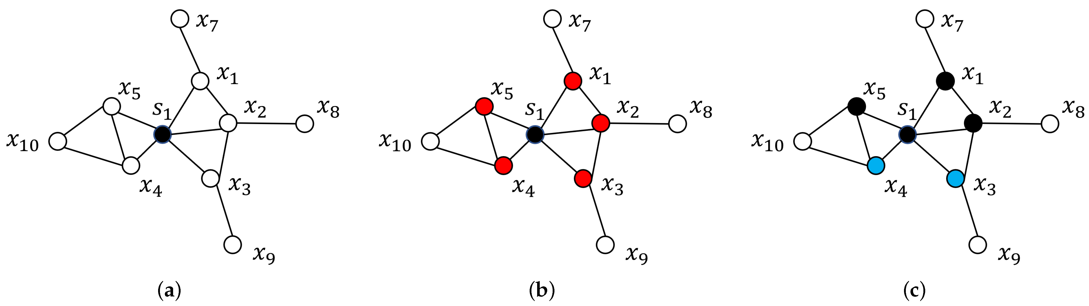
3.2. Shelved–Retrieved Method

To solve the WBCC model (1), the shelved–retrieved method embeds adjacent relationships into the construction of the power diagrams. This integration is essential for the generation of connected clusters.

It is crucial that clustering results remain connected throughout the process. Then, each point should be adjacent to at least one other point within the same cluster during the clustering procedure. In other words, they can only be assigned to clusters to which adjacent points belong. Here, we specify the assignment process for the shelved–retrieved method.

We take cluster one as an example. The shelved–retrieved method randomly selects a point from the dataset to serve as the initial site for cluster one. This selected point is assigned to cluster one and colored black in Figure 1a. Further, the adjacent hollow points of black points ${\mathit{s}}_1$, ${\mathit{x}}_1,{\mathit{x}}_2,{\mathit{x}}_3,{\mathit{x}}_4,{\mathit{x}}_5$ are identified and colored red in Figure 1b. According to parameters ${\alpha }_i,i=1,\dots ,n$, the shelved–retrieved method estimates whether $f{({\mathit{x}}_j,{\mathit{s}}_1)}^2-{\alpha }_1$ is smaller than $f{({\mathit{x}}_j,{\mathit{s}}_i)}^2-{\alpha }_i,i=2,\dots ,n$ at each point ${\mathit{x}}_j$. Assuming that $f{({\mathit{x}}_1,{\mathit{s}}_1)}^2-{\alpha }_1,f{({\mathit{x}}_2,{\mathit{s}}_1)}^2-{\alpha }_1,f{({\mathit{x}}_5,{\mathit{s}}_1)}^2-{\alpha }_1$ are the smallest and $f{({\mathit{x}}_3,{\mathit{s}}_1)}^2-{\alpha }_1,f{({\mathit{x}}_4,{\mathit{s}}_1)}^2-{\alpha }_1$ are not, the shelved–retrieved method assigns points ${\mathit{x}}_1,{\mathit{x}}_2,{\mathit{x}}_5$ to cluster one, and we color them black in Figure 1c. Points ${\mathit{x}}_3$ and ${\mathit{x}}_4$ are colored blue. The shelved–retrieved method repeats the aforementioned operations until no additional adjacent hollow points are identified.

Several blue and hollow points might not have been assigned to any cluster. These blue points are adjacent to other points within the same cluster during the clustering process. They are assigned to the clusters to which their adjacent points belong.

Using blue points ${\mathit{x}}_j$, the shelved–retrieved method identifies a set of clusters denoted by $\mathcal{A}=\{C_i:{\mathit{x}}_k\in C_i,{\mathit{x}}_k$ is a black point adjacent to ${\mathit{x}}_j\}$. The minimum $d{({\mathit{x}}_j,{\mathit{s}}_{i^{*}})}^2-{\alpha }_{i^{*}}$ is within the set $\{f{({\mathit{x}}_j,{\mathit{s}}_i)}^2-{\alpha }_i:{\mathit{s}}_i\in C_i,C_i\in \mathcal{A}\}$, while point ${\mathit{x}}_j$ is assigned to cluster $i^{*}$. The shelved–retrieved method repeats the process until all the points are turned black, as shown in Figure 1. Here, the aforementioned mechanism for clustering points with fixed parameters is concluded in Algorithm 1.

Algorithm 1 Clustering by power diagrams based on connectivity

Require: Domain $X=\{{\mathit{x}}_1,\dots ,{\mathit{x}}_m\}$, sites ${\mathit{s}}_1,\dots ,{\mathit{s}}_n$, parameters ${\alpha }_1,\dots ,{\alpha }_n$, adjacent set $A_{{\mathit{x}}_j},j=1,\dots ,m$ Ensure: Clustering solution $\mathcal{C}=\{C_1,\dots ,C_n\}$ 1: Initialize blue point set $B=\varnothing$, black point set $K=\varnothing$, red point set $R=\varnothing$, cluster $C_i=\left\{{\mathit{s}}_i\right\},i=1,\dots ,n$. 2: Update R based on $A_{{\mathit{s}}_i}$. 3: while$R\ne \varnothing$do 4:     for ${\mathit{x}}_j\in R$ do 5:         for $i=1,\dots ,n$ do 6:            if $i=\underset{i^{\prime }=1,\dots ,n}{argmin}f{({\mathit{x}}_j,{\mathit{s}}_{i^{\prime }})}^2-{\alpha }_{i^{\prime }}$ then 7:                Assign ${\mathit{x}}_j$ to $C_i$ and K, and update R based on $A_{{\mathit{x}}_j}$. 8:            end if 9:         end for 10:         if ${\mathit{x}}_j\notin K$ then 11:            Assign ${\mathit{x}}_j$ to B. 12:         end if 13:     end for 14:     if $R=\varnothing$ and $K\ne X$ then 15:         for ${\mathit{x}}_j\in B$ do 16:            Calculate $i=\underset{i^{\prime }\in \{C_i:C_i\cap K\cap A_{{\mathit{x}}_j}\ne \varnothing \}}{argmin}f{({\mathit{x}}_j,{\mathit{s}}_{i^{\prime }})}^2-{\alpha }_{i^{\prime }}$. 17:            Assign ${\mathit{x}}_j$ to $C_i$ and K, and update R based on $A_{{\mathit{x}}_j}$. 18:         end for 19:     end if 20: end while

The shelved–retrieved method uses Algorithm 2 to cluster the points. In each iteration, denoted by p, parameters ${\alpha }_i$ and $e_i:=\omega \left(C_i\right)-{\kappa }_i$ are represented by ${\alpha }_i^p$ and $e_i^p$, respectively. $\mathrm{sgn}(·)$ denotes the sign function. The sites can be updated by the Lloyd algorithm [25] in the clustering.

$${\alpha }_i^{p+1}=\left\{\begin{array}{cc}{\alpha }_i^p-0.1\mathrm{sgn}\left(e_i^p\right)\underset{j=1,\dots ,n,j\ne i}{min}d({\mathit{s}}_i,{\mathit{s}}_j)\hfill & ifp=1\hfill \\ {\alpha }_i^p-0.2\mathrm{sgn}\left(e_i^p\right)\underset{j=1,\dots ,n,j\ne i}{min}d({\mathit{s}}_i,{\mathit{s}}_j)/n\hfill & ifp\ge 2and({\alpha }_i^p-{\alpha }_i^{p-1})(e_i^p-e_i^{p-1})\ne 0\hfill \\ {\alpha }_i^p-min\left\{\left|\frac{{\alpha }_i^p-{\alpha }_i^{p-1}}{e_i^p-e_i^{p-1}}{e}_i^p\right|,0.2\underset{j=1,\dots ,n,j\ne i}{min}d({\mathit{s}}_i,{\mathit{s}}_j)/n\right\}\mathrm{sgn}\left(e_i^p\right)\hfill & \mathrm{otherwise}\hfill \end{array}\right..$$

(4)

Algorithm 2 Shelved-retrieved method

Require: Domain $X=\{{\mathit{x}}_1,\dots ,{\mathit{x}}_m\}$, weight set $\Omega =\{{\omega }_1,\dots ,{\omega }_m\}$, set $K=\{{\kappa }_1,\dots ,{\kappa }_n\}$, weight matrix $A_{\omega }$, adjacent set $A_{{\mathit{x}}_j}$ for each point ${\mathit{x}}_j$, and maximum number of iterations M. Ensure: Clustering solution $\mathcal{C}=\{C_1,\dots ,C_n\}$ 1: Initialize ${\mathit{s}}_1,\dots ,{\mathit{s}}_n$, ${\alpha }_1=0,\dots ,{\alpha }_n=0$. 2: repeat 3:     $p=1$ 4:     repeat 5:         Obtain the clustering $\mathcal{C}$ by the Algorithm 1. 6:         Update ${\alpha }_i^{p+1}$ by Formula (4) for each i. 7:         $p\leftarrow p+1$ 8:     until $p>M$ or $\mathcal{C}$ satisfies the constraints on cluster weights. 9:     Update ${\mathit{s}}_1,\dots ,{\mathit{s}}_n$ by the Lloyd algorithm. 10: until${\mathit{s}}_1,\dots ,{\mathit{s}}_n$ remain the same values.

Using the aforementioned process, the shelved–retrieved method can produce a connected solution for Model (1), as stated in Lemma 2.

Lemma 2. 

The shelved–retrieved method can produce a feasible solution for Model (1).

Proof. 

The shelved–retrieved method ensures that each point in a cluster is connected to the cluster site through a path, thereby resulting in connected clustering. Here, we prove that the clustering results satisfy the inequality constraints on the cluster weights.

For each cluster $C_i$, we can obtain point ${\mathit{x}}_j$ that satisfies

$$j=\underset{j:{\mathit{x}}_j\in C_i}{argmax}\frac{({\mathit{x}}_i-{\mathit{s}}_i)·({\mathit{s}}_k-{\mathit{s}}_i)}{f({\mathit{s}}_k,{\mathit{s}}_{\mathit{i}})}.$$

Based on the process of assigning points to the clusters, we propose the following inequality:

$${\alpha }_k-{\alpha }_i<f{({\mathit{x}}_j,{\mathit{s}}_k)}^2-f{({\mathit{x}}_j,{\mathit{s}}_{\mathit{i}})}^2,\forall e_{ik}\in E_s.$$

Further, we transform these inequalities into Standard equality system (5).

$$\begin{array}{ccc}\hfill {\alpha }_k^{\prime }-{\alpha }_k^{\prime \prime }-({\alpha }_i^{\prime }-{\alpha }_i^{\prime \prime })+{\beta }_{ik}& =f{({\mathit{x}}_j,{\mathit{s}}_k)}^2-f{({\mathit{x}}_j,{\mathit{s}}_{\mathit{i}})}^2,\hfill & \hfill \forall e_{ik}\in E_s\\ \hfill {\alpha }_i^{\prime },{\alpha }_i^{\prime \prime },{\beta }_{ik}& \ge 0,\hfill & \hfill \forall e_{ik}\in E_s\end{array}$$

(5)

The rank of the equality system is lower than $|E_s|$, both of which are smaller than the number of variables $2n+|E_s|$. Hence, Equality system (5) has a solution, and a power diagram is built.

By fixing the other parameters ${\alpha }_k,k\ne i$, the weight of cluster $C_i$ is within the interval $[\omega \left(s_i\right),{\sum }_{j=1}^m{\omega }_j]$. We consider cluster weight $\omega \left(C_i\right)$ as a response variable and parameter ${\alpha }_i$ as an independent variable. A step function is defined as the mapping from the independent variable to the response variable. Parameter ${\alpha }_i$ exists such that the corresponding cluster weight $\omega \left(C_i\right)$ in the step function satisfies the inequality constraint in Model (1). Because the sites are optimized using the shelved–retrieved method, clustering $\mathcal{C}$ produced by the shelved–retrieved method is the optimal solution for Model (1).    □

We offer the computational complexity analysis of Algorithm 2 as follows. In each iteration with a given red point set, Algorithm 1 handles these red points at most $O(mn\Delta (G\left)\right)$ times. Algorithm 1 loops through the red point set, at most, $m-n$ times; thus, the computation burden of Algorithm 1 is $O\left(\right(m-n)mn\Delta (G\left)\right)$. Algorithm 2 iterates, at most, $O(k_1{k}_2(m-n)mn\Delta \left(G\right))$ times, where $k_1$ denotes the number of site iterations and $k_2$ denotes the number of parameter iterations.

4. Results

We conducted the experiments on synthetic datasets and farmland consolidation with Windows 10, Intel(R) Core(TM) i7-10700K CPU @ 3.8GHz. The models were implemented using Python 3.8.5. To compare the results, we used two metrics for evaluation: the transportation costs (objective function value) and root-mean-square standard deviation (RMSSTD) [26]. A lower RMSSTD value indicates a better performance. RMSSTD was calculated using the following formula:

$$\mathrm{RMSSTD}={\left(\sum _{i=1}^n\frac{{\sum }_{{\mathit{x}}_j\in C_i}f{({\mathit{x}}_j,{\mathit{s}}_i)}^2}{d{\sum }_{i=1}^n\left(\right|C_i|-1)}\right)}^{\frac{1}{2}}.$$

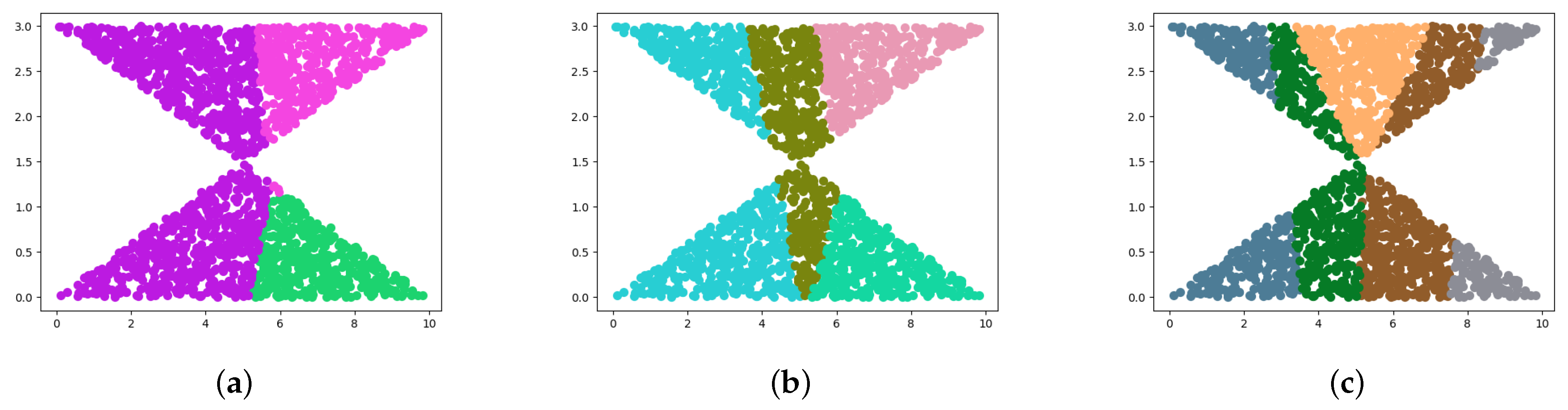
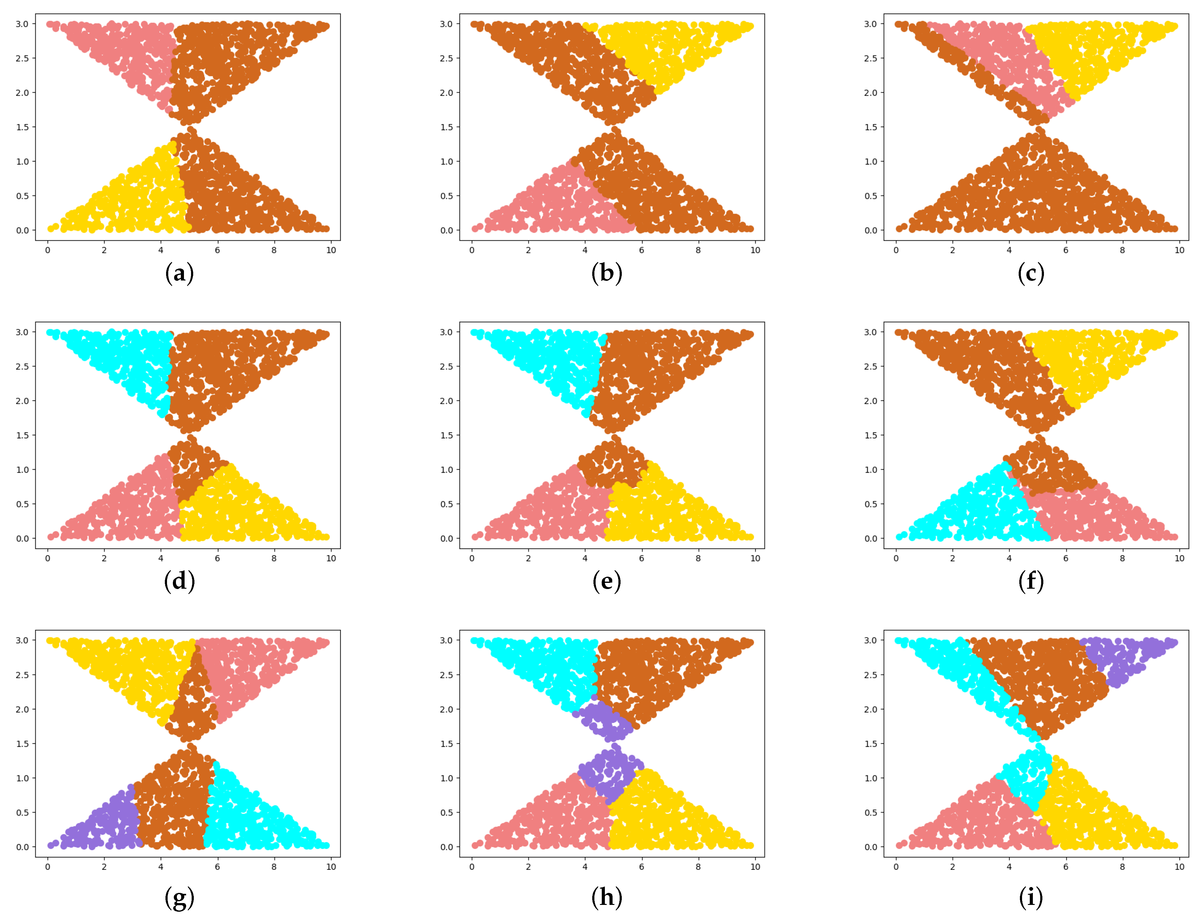
4.1. Synthetic Datasets

Experiments were conducted on three synthetic cases with three objective functions to evaluate the validity and rationality of the shelved–retrieved method. The discrete form of the centroidal power diagram (D-CPD) method, which is specified in Appendix A, was used as a comparison method in the experiments.

For all synthetic cases, 2000 points were generated in a funnel-shaped region, and chosen to effectively represent concave conditions. Three separate cases were constructed to evaluate the effectiveness of the proposed method on datasets containing different numbers of clusters. In Case 1, three subarea capacity intervals were set as [1969.49, 2089.49], [5819.85, 5939.85], and [2182.77, 2302.77]. In Case 2, we increased the number of subareas and the capacity intervals were set as [1969.49, 2089.49], [3819.85, 3939.85], [2182.77, 2302.77], and [1819.85, 2039.85]. In Case 3, we set five subareas with capacity intervals [1969.49, 2089.49], [2819.85, 2939.85], [2182.77, 2302.77], [1819.85, 2039.85], [819.85, 1045.85].

Transportation costs in different scenarios served as objective functions. Three distinct cost kernels were constructed to quantify different transportation costs and validate the effectiveness of our method across a range of scenarios.

First, the following Euclidean function was used as the cost kernel in the experiments as expressed below:

$${\widehat{f}}_1({\mathit{x}}_j,{\mathit{s}}_i)={\parallel {\mathit{x}}_j-{\mathit{s}}_i\parallel }_2.$$

In addition to the Euclidean function, two additional cost kernels, ${\widehat{f}}_2$ and ${\widehat{f}}_3$, were used in the experiments as expressed below:

$${\widehat{f}}_2(\mathit{x},\mathit{y})=(\mathit{x}-\mathit{y})M_1{(\mathit{x}-\mathit{y})}^T,$$

$${\widehat{f}}_3(\mathit{x},\mathit{y})=(\mathit{x}-\mathit{y})M_2{(\mathit{x}-\mathit{y})}^T.$$

Here,

$$M_1=\left(\begin{array}{cc}1& 0\\ 0& 4\end{array}\right)$$

is a positive-definite matrix, but

$$M_2=\left(\begin{array}{cc}1& 1\\ 2& 4\end{array}\right)$$

is not.

Because the D-CPD method is applicable exclusively in metric spaces, we applied it to address the WBCC problem with the cost kernel ${\widehat{f}}_1$. The results are shown in Figure 2. These results show that the D-CPD method yields disconnected results when applied to the synthetic datasets. Consequently, it can be inferred that the D-CPD method is unsuitable for solving the WBCC problem in all scenarios.

Further, the shelved–retrieved method was applied to address the WBCC problem. The results corresponding to the three distinct cost kernels are presented in Figure 3. The visual representations in Figure 3 show that our method consistently satisfies the connectivity requirements of the clusters. Hence, the shelved–retrieved method can produce connected results when applied in diverse scenarios.

To compare the shelved–retrieved method to the D-CPD method, we evaluated all the results using two metrics.

For each of the different cost kernels ${\widehat{f}}_k,k=1,2,3$, the transportation cost can be calculated using formula ${\sum }_{i=1}^n{\sum }_{{\mathit{x}}_j\in C_i}{\widehat{f}}_k$ for each k. The results are presented in

Table 2. Transportation costs of two methods on synthetic cases. Owing to the limitation of the D-CPD method to metric spaces, the transportation costs can only be calculated using the cost kernel ${\widehat{f}}_1$ in all the cases.

Case	Cost Kernel	Shelved–Retrieved Method	D-CPD Method	Reduction
	${\widehat{f}}_1$	2614.56	2615.82	0.0482%
Case 1	${\widehat{f}}_2$	3916.60	/	/
	${\widehat{f}}_3$	3040.00	/	/
	${\widehat{f}}_1$	2615.81	3319.67	21.20%
Case 2	${\widehat{f}}_2$	2635.42	/	/
	${\widehat{f}}_3$	2345.04	/	/
	${\widehat{f}}_1$	1881.07	3506.45	46.35%
Case 3	${\widehat{f}}_2$	2254.69	/	/
	${\widehat{f}}_3$	2069.65	/	/

. The transportation costs obtained using the shelved–retrieved method were considerably lower than those obtained using the D-CPD method. Compared to the D-CPD method, the transportation costs of the shelved–retrieved method were reduced by an average of 22.53% for the three cases. Consequently, the shelved–retrieved method effectively reduced transportation costs.

Additionally, we utilized RMSSTD as a metric to measure the similarity between the clusters.

All the results were evaluated using RMSSTD, and the values are presented in

Table 3. RMSSTD on synthetic cases. Since the D-CPD method can only be used in metric spaces, RMSSTD can be calculated with the objective function ${\widehat{f}}_1$ in all the cases.

Case	Cost Kernel	Shelved–Retrieved Method	D-CPD Method	Reduction
	${\widehat{f}}_1$	0.809	0.813	0.492%
Case 1	${\widehat{f}}_2$	0.99	/	/
	${\widehat{f}}_3$	0.87	/	/
	${\widehat{f}}_1$	0.74	0.91	18.68%
Case 2	${\widehat{f}}_2$	0.81	/	/
	${\widehat{f}}_3$	0.77	/	/
	${\widehat{f}}_1$	0.69	0.94	26.60%
Case 3	${\widehat{f}}_2$	0.75	/	/
	${\widehat{f}}_3$	0.72	/	/

. Table 3 shows that the RMSSTD of the shelved–retrieved method is considerably lower than that of the D-CPD method in each case. Consequently, the clustering results obtained using the shelved–retrieved method outperform those obtained using the D-CPD method.

In synthetic cases, compared with the D-CPD method, our method can produce connected and more compact clusters, and the corresponding transportation costs are much lower. The shelved–retrieved method is more suitable for solving the WBCC problems compared to the D-CPD method.

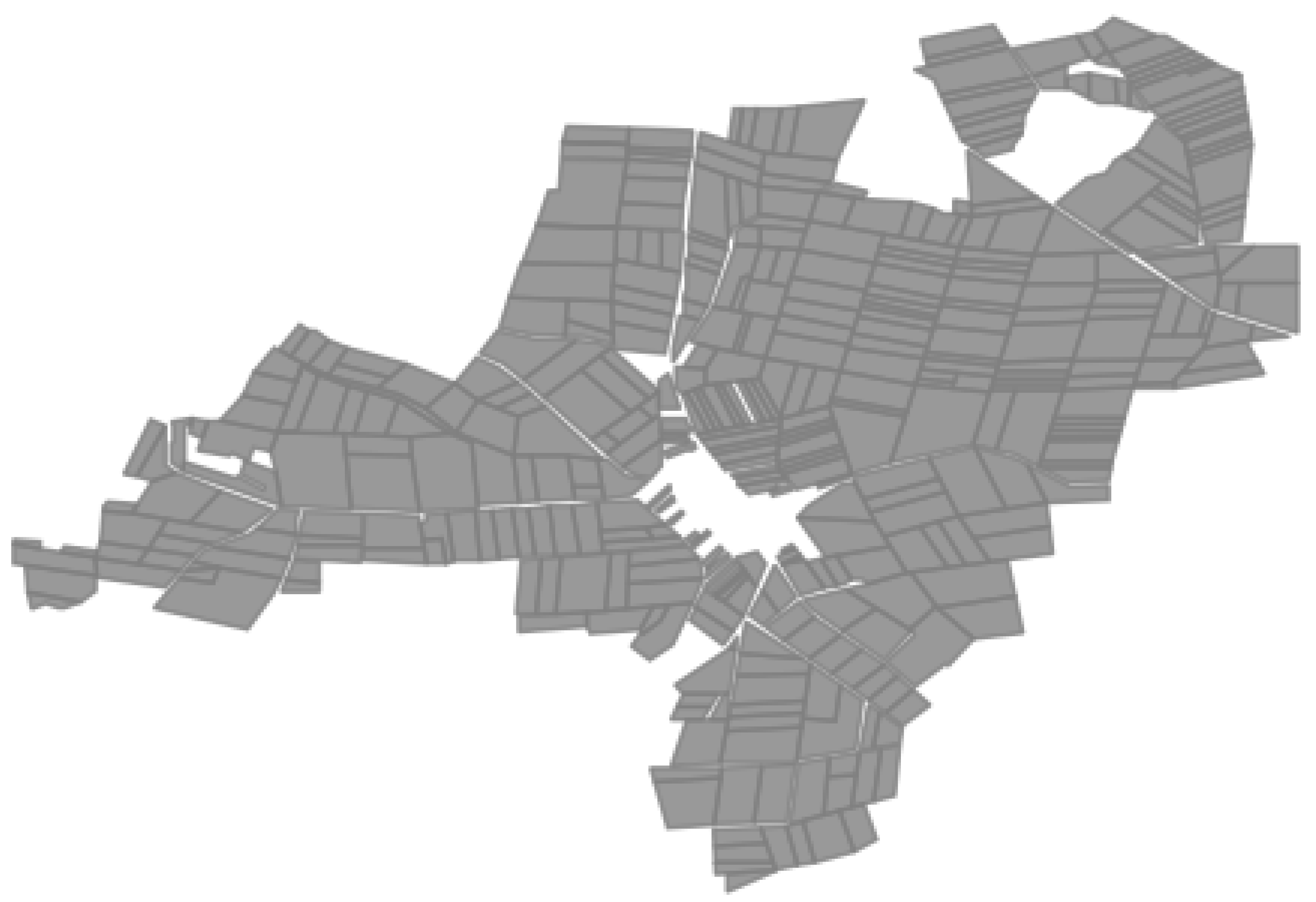
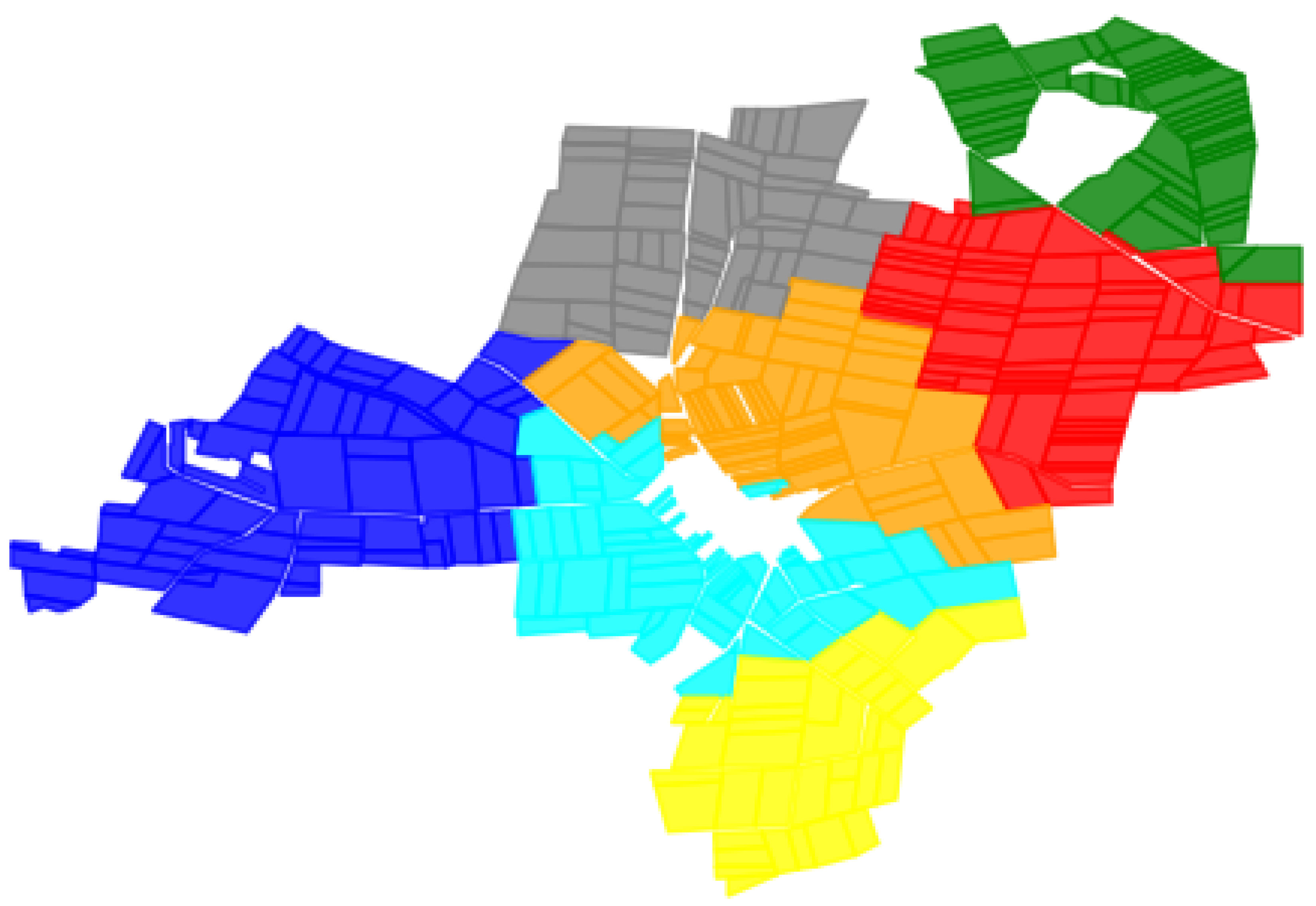
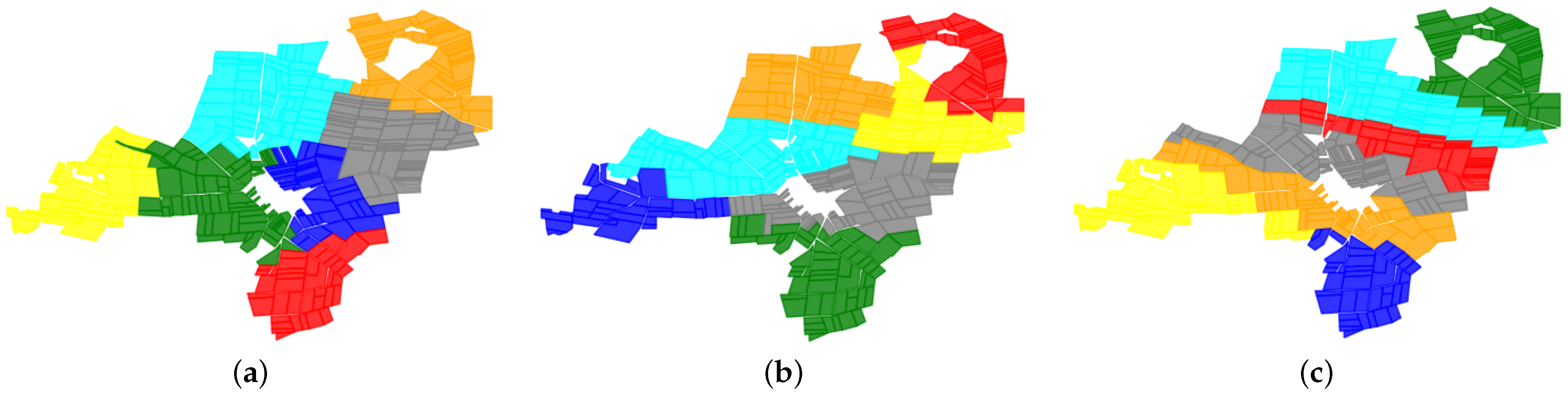
4.2. Farmland Consolidation

Farmland consolidation is a classical scenario in the WBCC. A large number of small-sized lots cultivated by farmers are scattered over an agricultural area. In farmland consolidation, these lots are restructured into several large connected fields. The adjacent lots in a large connected field are assigned to the same farmer, and the area of lots belonging to the farmer should not change too much. These requirements in farmland consolidation can be formulated by the WBCC problem.

To verify the rationality of our method, we conduct experiments on farmland consolidation. We obtain the relative data of the agricultural area in Germany, such as the position of each lot, the barriers in the area, and the boundary of the lots. Due to the privacy of the datasets, we present the schematic map of the agricultural area in Figure 4. As Figure 4 shows, the lots are distributed over a large area, and the barriers are located in the center of the farmland.

A total of 399 lots in Figure 4 are cultivated by seven farmers, and each farmer requires that the area should not change too much after reassignment. Each farmer, respectively, provides the lower and upper thresholds ${ϵ}^{-},{ϵ}^{+}$, i.e., the maximal value of area deviation. The original farm area of farmer i is denoted as ${\kappa }_i$; then, the restructured farmland area is within the interval $[{\kappa }_i-{ϵ}^{-},{\kappa }_i+{ϵ}^{+}]$. To harmonize expressions of formulation, we denote ${\kappa }_i^{-}={\kappa }_i-{ϵ}^{-}$ and ${\kappa }_i^{+}={\kappa }_i-{ϵ}^{+}$.

According to the requirements in farmland consolidation, information regarding the belonging of each lot to respective farmers should be obtained. In the experiments, we set $m=7$ and $n=399$. Similar to the experiments on synthetic datasets, the D-CPD method is applied to handle the farmland consolidation with cost kernel ${\widehat{f}}_1$. As presented in Figure 5, the D-CPD method produces a disconnected result in the cyan cluster. Hence, the D-CPD method is unsuitable for solving the WBCC problem in farmland consolidation.

Furthermore, the shelved–retrieved method is applied to solve the farmland consolidation with $r=18$ in the experiments. Three cost kernels ${\widehat{f}}_1,{\widehat{f}}_2,\widehat{f_3}$ are used to measure different transportation costs in farmland consolidation. The results corresponding to the three distinct objective functions are shown in Figure 6. Compared with the result of the D-CPD method in Figure 5, the shelved–retrieved method produces connected results but the D-CPD method does not. Thus, the shelved–retrieved method can reasonably solve the WBCC problem in farmland consolidation.

We also evaluate all results by the transportation costs and RMSSTD to compare the two methods. Transportation costs are presented in

Table 4. Transportation costs of two methods on farmland consolidation. Owing to the limitation of the D-CPD method to metric spaces, the transportation costs can only be calculated using the objective function ${\widehat{f}}_1$ in all the cases.

Cost Kernel	Shelved–Retrieved Method	D-CPD Method
${\widehat{f}}_1$	8239.77	13,772.06
${\widehat{f}}_2$	9711.75	/
${\widehat{f}}_3$	10,538.33	/

. In the experiments, the transportation cost generated by the results of the shelved–retrieved method is reduced by 40.17% compared to the D-CPD method. Therefore, the shelved–retrieved method can reduce the cost of equipment transportation between lots.

The RMSSTD value of each result is presented in

Table 5. RMSSTD of two methods on farmland consolidation. Owing to the limitation of the D-CPD method to metric spaces, the transportation costs can only be calculated using the objective function ${\widehat{f}}_1$ in all the cases.

Cost Kernel	Shelved–Retrieved Method	D-CPD Method
${\widehat{f}}_1$	3.24	4.19
${\widehat{f}}_2$	3.46	/
${\widehat{f}}_3$	3.67	/

. Table 5 shows that the RMSSTD of the shelved–retrieved method is lower than that of the D-CPD method with a 22.67% reduction. Thus, the shelved–retrieved method outperforms other methods in farmland consolidation.

5. Conclusions

The WBCC problem necessitates the division of a point set into connected clusters, each with weights falling within specified intervals. To handle this problem, our study introduced the shelved–retrieved method, which incorporates adjacent relationships into power diagram construction, enabling points to be assigned to clusters based on their adjacent points. Leveraging parameters from power diagrams, this method effectively partitions the point set into connected clusters. Furthermore, it employs a specially designed loop structure to guarantee the generation of clusters that adhere to both weight and geometrical connectivity constraints.

Our experiments, which included three synthetic cases using three cost kernels, as well as their application in farmland consolidation, consistently demonstrated the effectiveness of the shelved–retrieved method. Our results consistently met the constraints of the WBCC problem, resulting in an average reduction of transportation costs by 22.53% and 40.17% for synthetic cases and farmland consolidation, respectively.

Our findings highlight the fact that the shelved–retrieved method not only addresses the WBCC problem effectively, but also ensures cluster connectivity, surpassing other techniques in terms of transportation costs and RMSSTD. This method’s flexibility in quantifying different costs through cost kernels allows for substantial cost reductions in various scenarios. However, it is important to note that the shelved–retrieved method may face challenges when dealing with high-dimensional weights. Future research endeavors should aim to address the WBCC problem in such high-dimensional weight scenarios to further enhance the method’s applicability and effectiveness.

References

1. Jain, A.K.; Murty, M.N.; Flynn, P.J. Data clustering: A review. ACM Comput. Surv. (CSUR) 1999, 31, 264–323. [Google Scholar] [CrossRef]
2. Omran, M.G.H.; Engelbrecht, A.P.; Salman, A. An overview of clustering methods. Intell. Data Anal. 2007, 11, 583–605. [Google Scholar] [CrossRef]
3. Stillwell, M.; Schanzenbach, D.; Vivien, F.; Casanova, H. Resource allocation using virtual clusters. In Proceedings of the 2009 9th IEEE/ACM International Symposium on Cluster Computing and the Grid, Shanghai, China, 18–21 May 2009; pp. 260–267. [Google Scholar]
4. Fischer, D.T.; Church, R.L. Clustering and compactness in reserve site selection: An extension of the biodiversity management area selection model. For. Sci. 2003, 49, 555–565. [Google Scholar]
5. Yang, K.; Shekhar, A.H.; Oliver, D.; Shekhar, S. Capacity-constrained network-voronoi diagram. IEEE Trans. Knowl. Data Eng. 2015, 27, 2919–2932. [Google Scholar] [CrossRef]
6. Chopra, S.; Rao, M.R. The partition problem. Math. Program. 1993, 59, 87–115. [Google Scholar] [CrossRef]
7. Baranwal, M.; Salapaka, S.M. Clustering with capacity and size constraints: A deterministic approach. In Proceedings of the 2017 Indian Control Conference (ICC), Guwahati, India, 4–6 January 2017; pp. 251–256. [Google Scholar]
8. Brieden, A.; Gritzmann, P.; Klemm, F. Constrained clustering via diagrams: A unified theory and its application to electoral district design. Eur. J. Oper. Res. 2017, 263, 18–34. [Google Scholar] [CrossRef]
9. Brieden, A.; Gritzmann, P. On optimal weighted balanced clusterings: Gravity bodies and power diagrams. SIAM J. Discret. Math. 2012, 26, 415–434. [Google Scholar] [CrossRef]
10. Borgwardt, S.; Brieden, A.; Gritzmann, P. Geometric clustering for the consolidation of farmland and woodland. Math. Intell. 2014, 36, 37–44. [Google Scholar] [CrossRef]
11. Bradley, P.S.; Bennett, K.P.; Demiriz, A. Constrained k-means clustering. Microsoft Res. Redmond 2000, 20. Available online: https://www.microsoft.com/en-us/research/wp-content/uploads/2016/02/tr-2000-65.pdf (accessed on 15 October 2023).
12. Brieden, A.; Gritzmann, P. A quadratic optimization model for the consolidation of farmland by means of lend-lease agreements. In Operations Research Proceedings 2003; Springer: Berlin/Heidelberg, Germany, 2004; pp. 324–331. [Google Scholar]
13. Borgwardt, S.; Brieden, A.; Gritzmann, P. Constrained minimum-k-star clustering and its application to the consolidation of farmland. Oper. Res. 2011, 11, 1–17. [Google Scholar] [CrossRef]
14. Ganganath, N.; Cheng, C.; Chi, K.T. Data clustering with cluster size constraints using a modified k-means algorithm. In Proceedings of the 2014 International Conference on Cyber-Enabled Distributed Computing and Knowledge Discovery, Shanghai, China, 13–15 October 2014; pp. 158–161. [Google Scholar]
15. Höppner, F.; Klawonn, F. Clustering with size constraints. In Computational Intelligence Paradigms Innovative Applications; Springer: Berlin/Heidelberg, Germany, 2008; pp. 167–180. [Google Scholar]
16. Zhu, S.; Wang, D.; Li, T. Data clustering with size constraints. Knowl.-Based Syst. 2010, 23, 883–889. [Google Scholar] [CrossRef]
17. Rose, K. Deterministic Annealing, Clustering, and Optimization; California Institute of Technology: Pasadena, CA, USA, 1991. [Google Scholar]
18. Hu, C.W.; Li, H.; Qutub, A.A. Shrinkage clustering: A fast and size-constrained clustering algorithm for biomedical applications. BMC Bioinform. 2018, 19, 19. [Google Scholar] [CrossRef] [PubMed]
19. Li, J.; Horiguchi, Y.; Sawaragi, T. Cluster size-constrained fuzzy c-means with density center searching. Int. J. Fuzzy Log. Intell. Syst. 2020, 20, 346–357. [Google Scholar] [CrossRef]
20. Tang, W.; Yang, Y.; Zeng, L.; Zhan, Y. Size constrained clustering with milp formulation. IEEE Access 2020, 8, 1587–1599. [Google Scholar] [CrossRef]
21. Balzer, M. Capacity-constrained voronoi diagrams in continuous spaces. In Proceedings of the 2009 Sixth International Symposium on Voronoi Diagrams, Copenhagen, Denmark, 23–26 June 2009; pp. 79–88. [Google Scholar]
22. Xin, S.; Lévy, B.; Chen, Z.; Chu, L.; Yu, Y.; Tu, C.; Wang, W. Centroidal power diagrams with capacity constraints: Computation, applications, and extension. ACM Trans. Graph. (TOG) 2016, 35, 1–12. [Google Scholar] [CrossRef]
23. Galvao, L.C.; Novaes, A.G.; De Cursi, J.S.; Souza, J.C. A multiplicatively-weighted voronoi diagram approach to logistics districting. Comput. Oper. Res. 2006, 33, 93–114. [Google Scholar] [CrossRef]
24. Aurenhammer, F.; Hoffmann, F.; Aronov, B. Minkowski-type theorems and least-squares clustering. Algorithmica 1998, 20, 61–76. [Google Scholar] [CrossRef]
25. Lloyd, S. Least squares quantization in PCM. IEEE Trans. Inf. Theory 1982, 28, 129–137. [Google Scholar] [CrossRef]
26. Liu, Y.; Li, Z.; Xiong, H.; Gao, X.; Wu, J. Understanding of internal clustering validation measures. In Proceedings of the 2010 IEEE International Conference on Data Mining, Sydney, Australia, 13 December 2010; pp. 911–916. [Google Scholar]
Figure 1. The assigning process of the shelved–retrieved method: The black, hollow, red, and blue points represent those that belong to clusters, have not undergone processing yet, are eligible candidates for assignment to clusters, and are temporarily unassigned to any clusters, respectively. (a) Initial state; (b) Finding the adjacent points; (c) Assigning points.
Algorithms 16 00492 g001
Figure 2. Results on the three synthetic cases. In each subfigure, the color of a point represents the cluster to which it belongs. (a) The result in Case 1; (b) The result in Case 2; (c) The result in Case 3.
Algorithms 16 00492 g002
Figure 3. (ai) Results of three synthetic cases with three cost kernels. In each subfigure, the color of a point represents the cluster to which it belongs. The results in the same row represent variations of a single case under different cost kernel functions, while those in the same column correspond to a common cost kernel. The cost kernels involved in the three columns are f ^ 1 ( x , y ) = x y 2 , f ^ 2 ( x , y ) = ( x y ) M 1 ( x y ) T , and f ^ 3 ( x , y ) = ( x y ) M 2 ( x y ) T , respectively.
Algorithms 16 00492 g003
Figure 4. The schematic map of the agricultural area in German.
Algorithms 16 00492 g004
Figure 5. Results on farmland consolidation by the D-CPD method. The color of a point represents the cluster to which it belongs.
Algorithms 16 00492 g005
Figure 6. Results on the farmland consolidation with three cost kernels. The color of a point represents the cluster to which it belongs. (a) The result with cost kernel f ^ 1 ; (b) The result with cost kernel f ^ 2 ; (c) The result with cost kernel f ^ 3 .
Algorithms 16 00492 g006