
Exploring Graph and Digraph Persistence


Abstract
1. Introduction
Organization of the Paper
2. State of the Art
2.1. Generalizations of Persistence
2.2. Persistent Homology for (Di)graphs
3. Graph-Theoretical Persistence
3.1. Categorical Persistence Functions
- and ;
- .
3.2. Indexing-Aware Persistence Functions
- For any (di)graphs and any , in implies that in .
- In any (di)graph , for any , implies that .
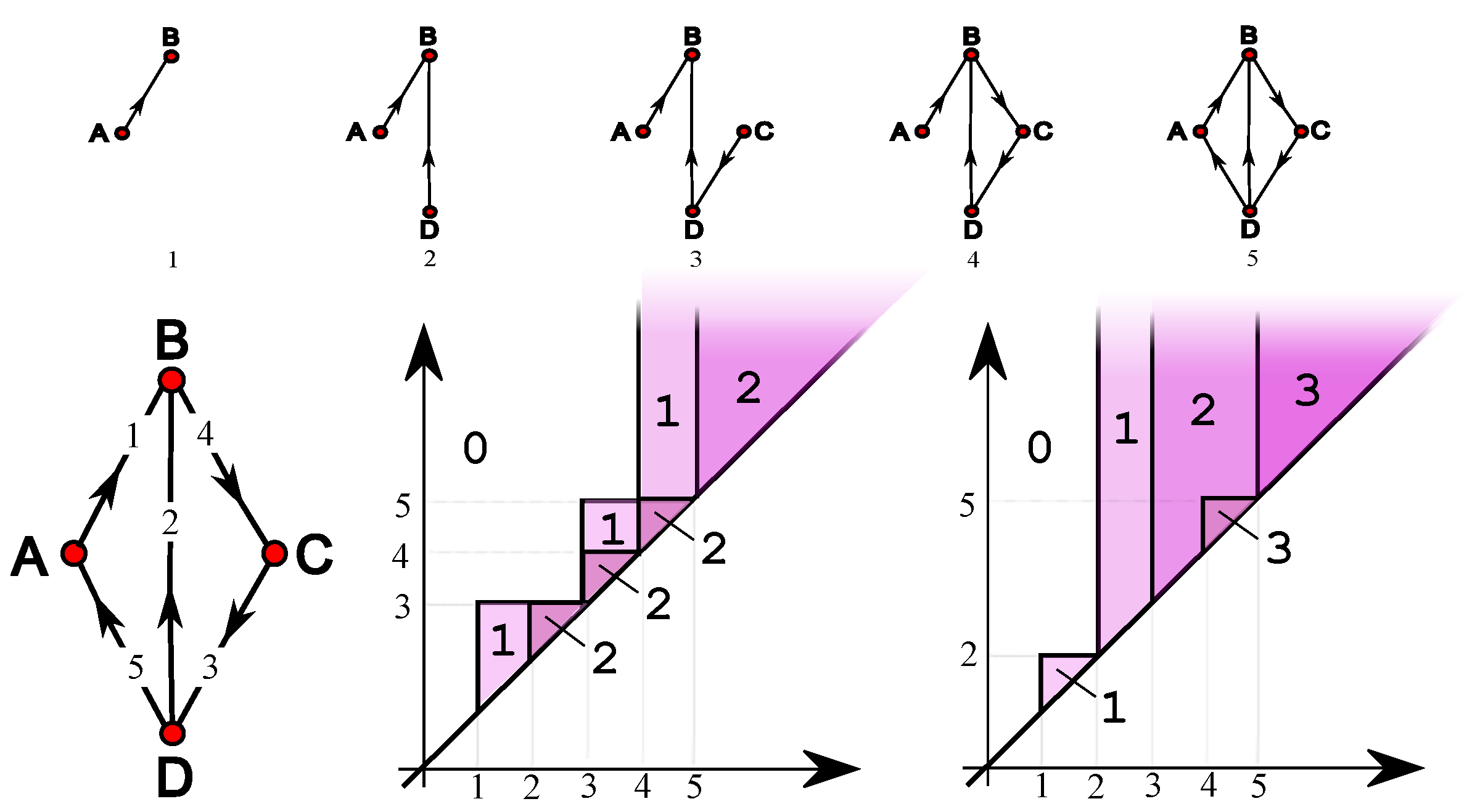
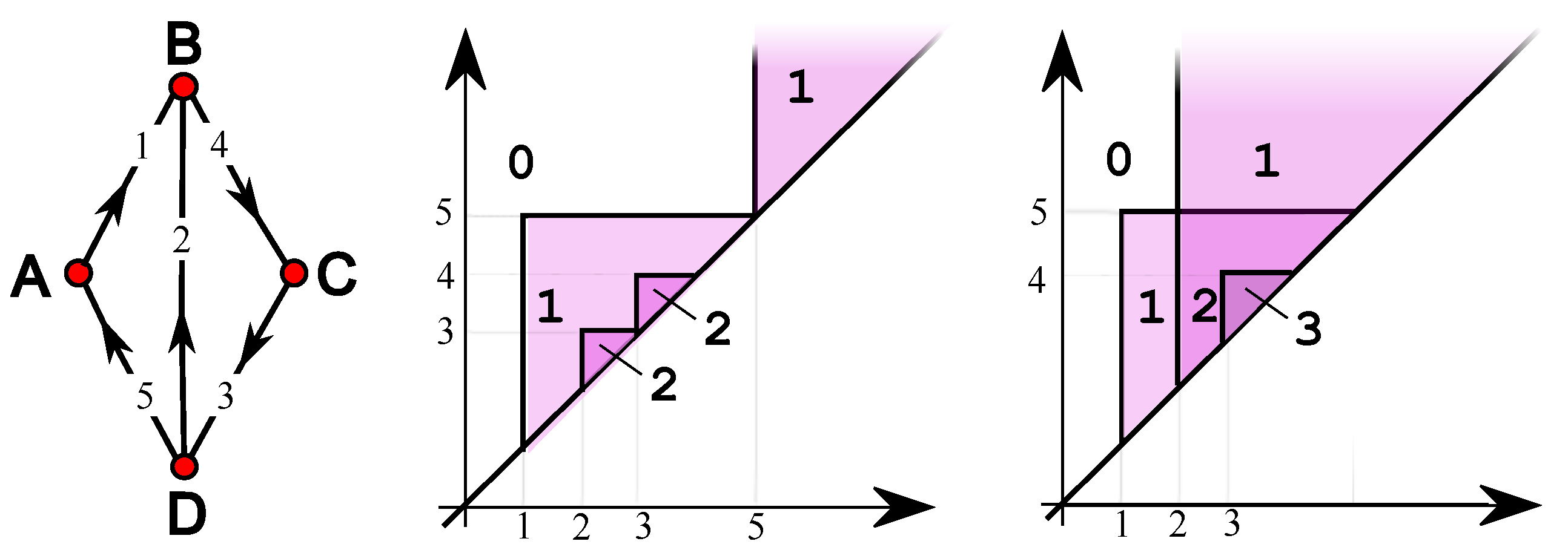
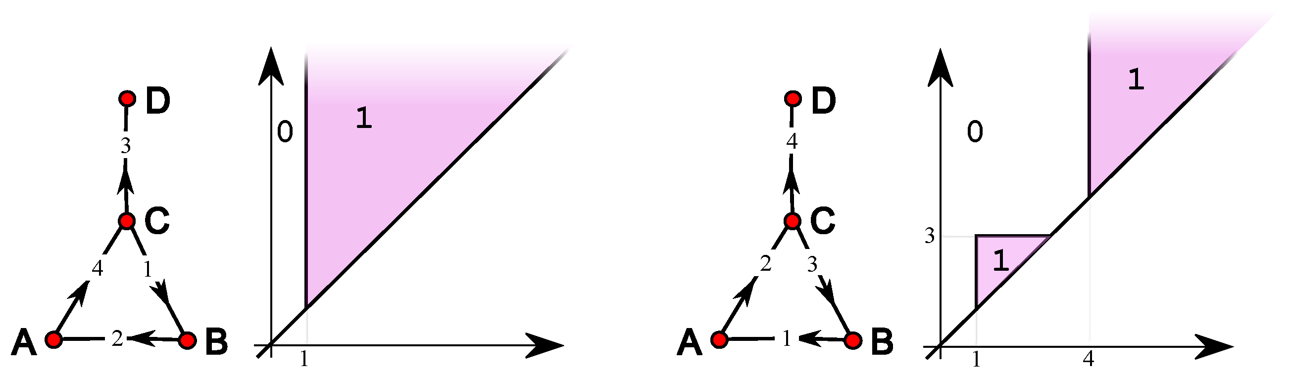
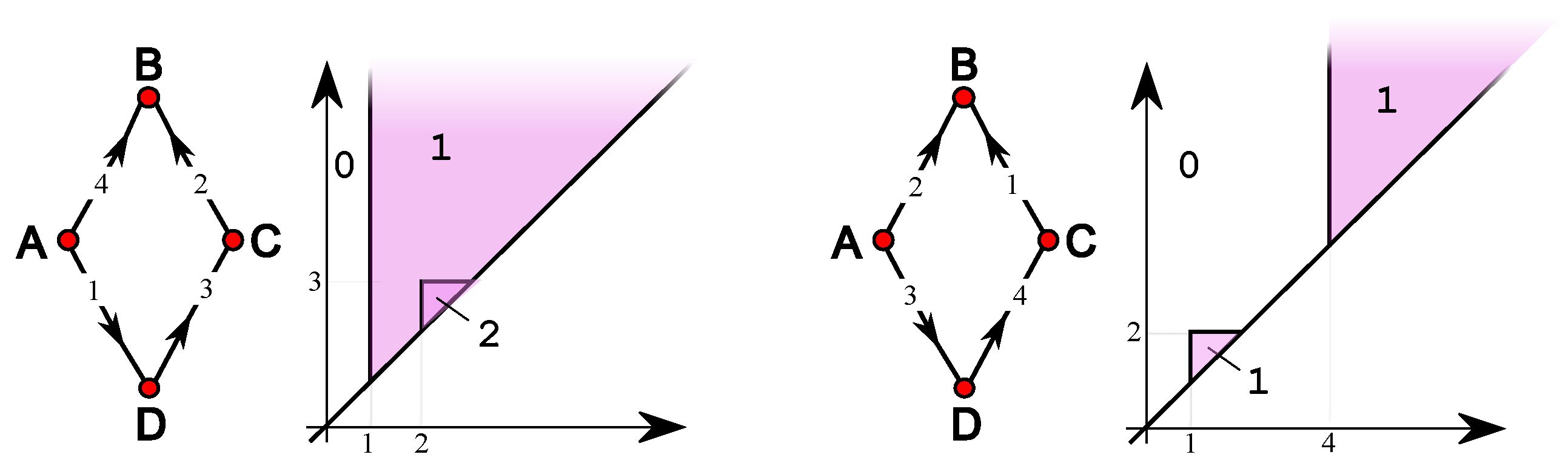
4. Simple Features
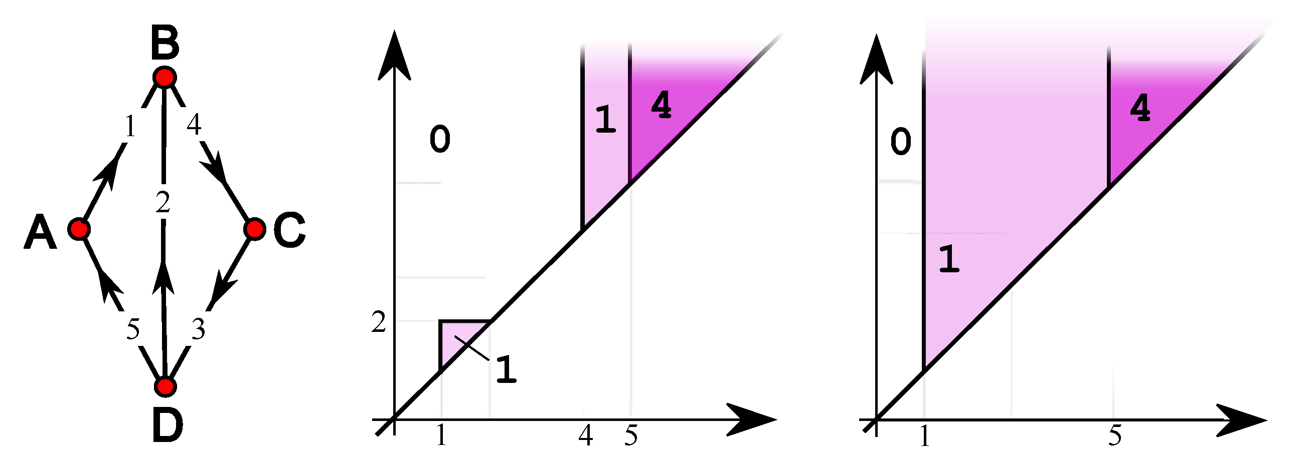
5. Single-Vertex Features
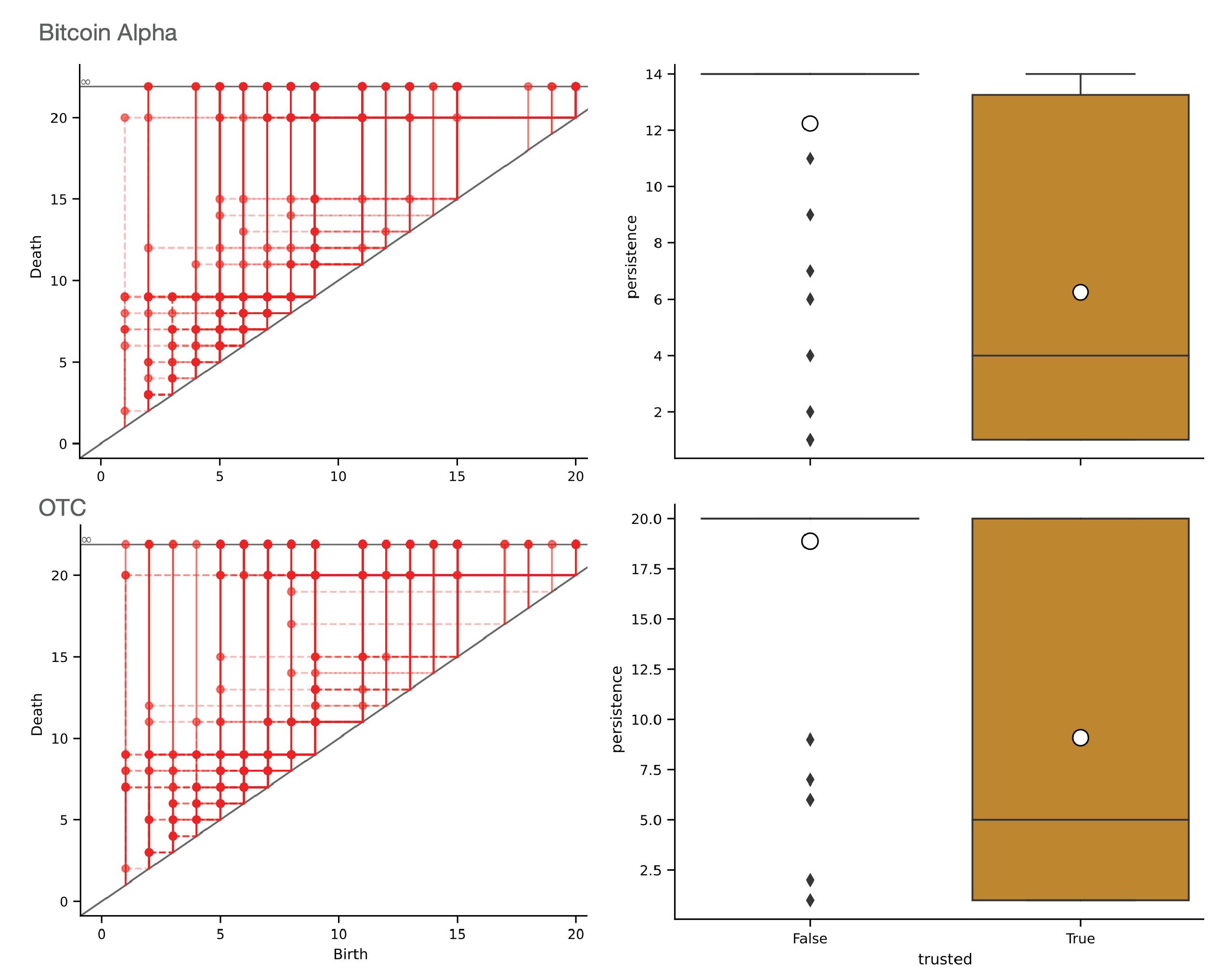
6. Computational Experiments
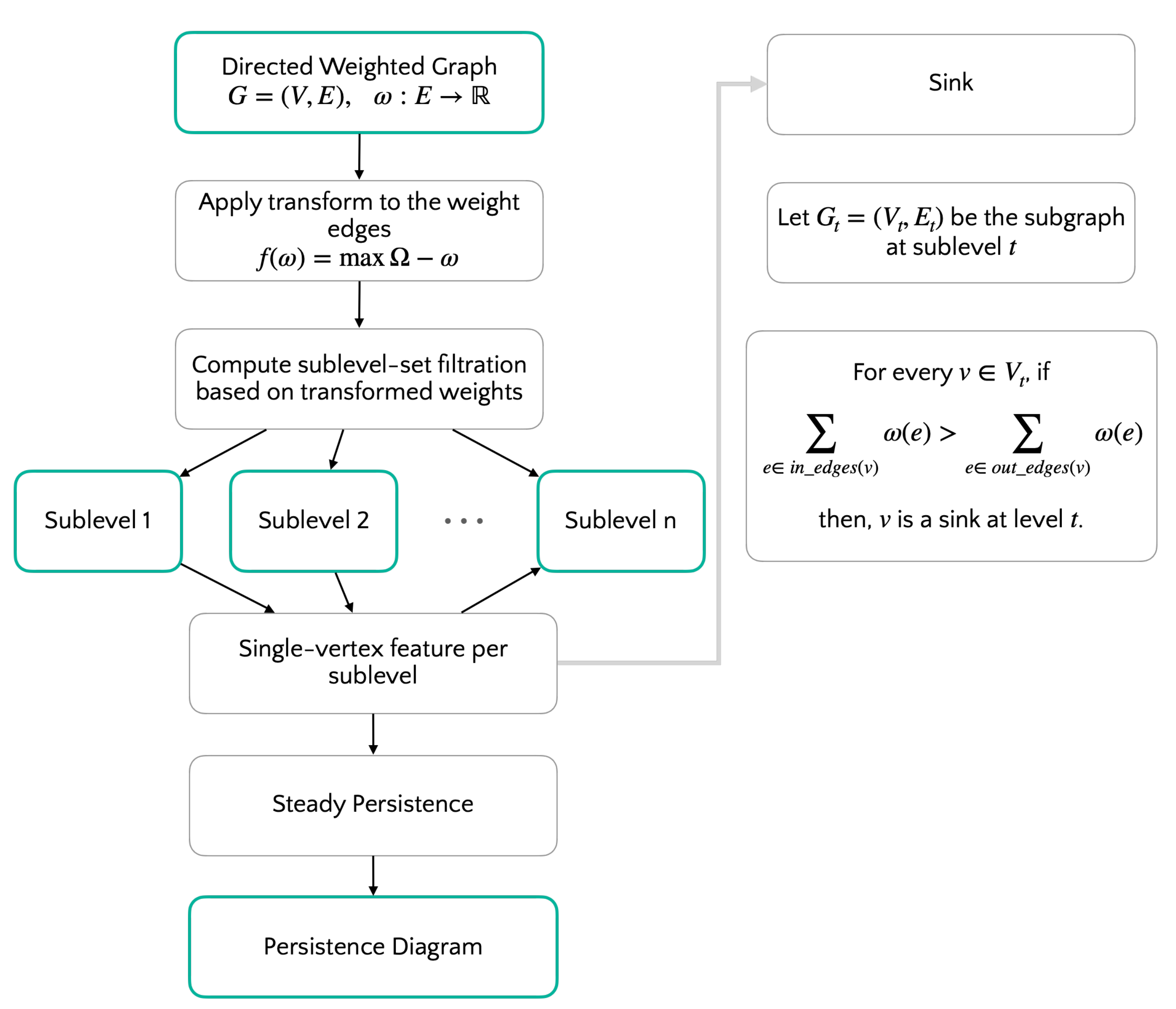
6.1. Algorithm
6.2. Datasets
6.3. Results
7. Discussion
8. Conclusions
Author Contributions
Funding
Data Availability Statement
Acknowledgments
Conflicts of Interest
Appendix A. Unbalanced


References
- Otter, N.; Porter, M.A.; Tillmann, U.; Grindrod, P.; Harrington, H.A. A roadmap for the computation of persistent homology. EPJ Data Sci. 2017, 6, 1–38. [Google Scholar] [CrossRef] [PubMed]
- Cohen-Steiner, D.; Edelsbrunner, H.; Harer, J. Stability of persistence diagrams. In Proceedings of the Symposium on Computational Geometry, Pisa, Italy, 6–8 June 2005; Mitchell, J.S.B., Rote, G., Eds.; ACM: New York, NY, USA, 2005; pp. 263–271. [Google Scholar]
- Lesnick, M. The Theory of the Interleaving Distance on Multidimensional Persistence Modules. Found. Comput. Math. 2015, 15, 613–650. [Google Scholar] [CrossRef]
- Di Fabio, B.; Landi, C. A Mayer–Vietoris formula for persistent homology with an application to shape recognition in the presence of occlusions. Found. Comput. Math. 2011, 11, 499–527. [Google Scholar] [CrossRef][Green Version]
- Malott, N.O.; Chen, S.; Wilsey, P.A. A survey on the high-performance computation of persistent homology. IEEE Trans. Knowl. Data Eng. 2022, 35, 4466–4484. [Google Scholar] [CrossRef]
- Bergomi, M.G.; Vertechi, P. Rank-based persistence. Theory Appl. Categ. 2020, 35, 228–260. [Google Scholar]
- Bergomi, M.G.; Ferri, M.; Vertechi, P.; Zuffi, L. Beyond Topological Persistence: Starting from Networks. Mathematics 2021, 9, 3079. [Google Scholar] [CrossRef]
- Bergomi, M.G.; Ferri, M.; Tavaglione, A. Steady and ranging sets in graph persistence. J. Appl. Comput. Topol. 2022, 7, 33–56. [Google Scholar] [CrossRef]
- Bergomi, M.G.; Ferri, M.; Mella, A.; Vertechi, P. Generalized Persistence for Equivariant Operators in Machine Learning. Mach. Learn. Knowl. Extr. 2023, 5, 346–358. [Google Scholar] [CrossRef]
- Monti, F.; Otness, K.; Bronstein, M.M. Motifnet: A motif-based graph convolutional network for directed graphs. In Proceedings of the 2018 IEEE Data Science Workshop (DSW), Lausanne, Switzerland, 4–6 June 2018; IEEE: Piscataway, NJ, USA, 2018; pp. 225–228. [Google Scholar]
- Tong, Z.; Liang, Y.; Sun, C.; Rosenblum, D.S.; Lim, A. Directed graph convolutional network. arXiv 2020, arXiv:2004.13970. [Google Scholar]
- Zhang, X.; He, Y.; Brugnone, N.; Perlmutter, M.; Hirn, M. Magnet: A neural network for directed graphs. Adv. Neural Inf. Process. Syst. 2021, 34, 27003–27015. [Google Scholar]
- Estrada, E. The Structure of Complex Networks: Theory and Applications; Oxford University Press: New York, NY, USA, 2012. [Google Scholar]
- Zhao, S.X.; Fred, Y.Y. Exploring the directed h-degree in directed weighted networks. J. Inf. 2012, 6, 619–630. [Google Scholar] [CrossRef]
- Yang, Y.; Xie, G.; Xie, J. Mining important nodes in directed weighted complex networks. Discret. Dyn. Nat. Soc. 2017, 2017, 9741824. [Google Scholar] [CrossRef]
- Carlsson, G. Topology and data. Bull. Amer. Math. Soc. 2009, 46, 255–308. [Google Scholar] [CrossRef]
- Carlsson, G.; Singh, G.; Zomorodian, A. Computing Multidimensional Persistence. In Proceedings of the ISAAC, Honolulu, HI, USA, 16–18 December 2009; Dong, Y., Du, D.Z., Ibarra, O.H., Eds.; Springer: Berlin/Heidelberg, Germany, 2009. Lecture Notes in Computer Science. Volume 5878, pp. 730–739. [Google Scholar]
- Burghelea, D.; Dey, T.K. Topological persistence for circle-valued maps. Discret. Comput. Geom. 2013, 50, 69–98. [Google Scholar] [CrossRef]
- Bubenik, P.; Scott, J.A. Categorification of persistent homology. Discret. Comput. Geom. 2014, 51, 600–627. [Google Scholar] [CrossRef]
- de Silva, V.; Munch, E.; Stefanou, A. Theory of interleavings on categories with a flow. Theory Appl. Categ. 2018, 33, 583–607. [Google Scholar]
- Kim, W.; Mémoli, F. Generalized persistence diagrams for persistence modules over posets. J. Appl. Comput. Topol. 2021, 5, 533–581. [Google Scholar] [CrossRef]
- McCleary, A.; Patel, A. Edit Distance and Persistence Diagrams Over Lattices. SIAM J. Appl. Algebra Geom. 2022, 6, 134–155. [Google Scholar] [CrossRef]
- Mémoli, F.; Wan, Z.; Wang, Y. Persistent Laplacians: Properties, algorithms and implications. SIAM J. Math. Data Sci. 2022, 4, 858–884. [Google Scholar] [CrossRef]
- Southern, J.; Wayland, J.; Bronstein, M.; Rieck, B. Curvature filtrations for graph generative model evaluation. arXiv 2023, arXiv:2301.12906. [Google Scholar]
- Watanabe, S.; Yamana, H. Topological measurement of deep neural networks using persistent homology. Ann. Math. Artif. Intell. 2022, 90, 75–92. [Google Scholar] [CrossRef]
- Ju, H.; Zhou, D.; Blevins, A.S.; Lydon-Staley, D.M.; Kaplan, J.; Tuma, J.R.; Bassett, D.S. Historical growth of concept networks in Wikipedia. Collect. Intell. 2022, 1, 26339137221109839. [Google Scholar] [CrossRef]
- Arfi, B. The promises of persistent homology, machine learning, and deep neural networks in topological data analysis of democracy survival. Qual. Quant. 2023. [Google Scholar] [CrossRef]
- Sizemore, A.E.; Giusti, C.; Kahn, A.; Vettel, J.M.; Betzel, R.F.; Bassett, D.S. Cliques and cavities in the human connectome. J. Comput. Neurosci. 2018, 44, 115–145. [Google Scholar] [CrossRef] [PubMed]
- Guerra, M.; De Gregorio, A.; Fugacci, U.; Petri, G.; Vaccarino, F. Homological scaffold via minimal homology bases. Sci. Rep. 2021, 11, 5355. [Google Scholar] [CrossRef]
- Rieck, B.; Fugacci, U.; Lukasczyk, J.; Leitte, H. Clique community persistence: A topological visual analysis approach for complex networks. IEEE Trans. Vis. Comput. Graph. 2018, 24, 822–831. [Google Scholar] [CrossRef] [PubMed]
- Aktas, M.E.; Akbas, E.; Fatmaoui, A.E. Persistence homology of networks: Methods and applications. Appl. Netw. Sci. 2019, 4, 61. [Google Scholar] [CrossRef]
- Reimann, M.W.; Nolte, M.; Scolamiero, M.; Turner, K.; Perin, R.; Chindemi, G.; Dłotko, P.; Levi, R.; Hess, K.; Markram, H. Cliques of Neurons Bound into Cavities Provide a Missing Link between Structure and Function. Front. Comput. Neurosci. 2017, 11, 48. [Google Scholar] [CrossRef]
- Chowdhury, S.; Mémoli, F. Persistent path homology of directed networks. In Proceedings of the Twenty-Ninth Annual ACM-SIAM Symposium on Discrete Algorithms, New Orleans, LA, USA, 7–10 January 2018; SIAM: Philadelphia, PA, USA, 2018; pp. 1152–1169. [Google Scholar]
- Dey, T.K.; Li, T.; Wang, Y. An efficient algorithm for 1-dimensional (persistent) path homology. Discret. Comput. Geom. 2022, 68, 1102–1132. [Google Scholar] [CrossRef]
- Loday, J.L. Cyclic Homology; Springer Science & Business Media: Berlin/Heidelberg, Germany, 2013; Volume 301. [Google Scholar]
- Caputi, L.; Riihimäki, H. Hochschild homology, and a persistent approach via connectivity digraphs. J. Appl. Comput. Topol. 2023, 1–50. [Google Scholar] [CrossRef]
- Edelsbrunner, H.; Harer, J. Persistent homology—A survey. In Surveys on Discrete and Computational Geometry; American Mathematical Society: Providence, RI, USA, 2008; Volume 453, pp. 257–282. [Google Scholar]
- Edelsbrunner, H.; Harer, J. Computational Topology: An Introduction; American Mathematical Society: Providence, RI, USA, 2009. [Google Scholar]
- Mella, A. Non-Topological Persistence for Data Analysis and Machine Learning. Ph.D. Thesis, Alma Mater Studiorum-Università di Bologna, Bologna, Italy, 2021. [Google Scholar]
- Kumar, S.; Spezzano, F.; Subrahmanian, V.; Faloutsos, C. Edge weight prediction in weighted signed networks. In Proceedings of the 2016 IEEE 16th International Conference on Data Mining (ICDM), Barcelona, Spain, 12–15 December 2016; IEEE: Piscataway, NJ, USA, 2016; pp. 221–230. [Google Scholar]
- Colombo, G.; Cubero, R.J.A.; Kanari, L.; Venturino, A.; Schulz, R.; Scolamiero, M.; Agerberg, J.; Mathys, H.; Tsai, L.H.; Chachólski, W.; et al. A tool for mapping microglial morphology, morphOMICs, reveals brain-region and sex-dependent phenotypes. Nat. Neurosci. 2022, 25, 1379–1393. [Google Scholar] [CrossRef]
- Wee, J.; Xia, K. Persistent spectral based ensemble learning (PerSpect-EL) for protein–protein binding affinity prediction. Briefings Bioinform. 2022, 23, bbac024. [Google Scholar] [CrossRef]
- Qiu, Y.; Wei, G.W. Artificial intelligence-aided protein engineering: From topological data analysis to deep protein language models. arXiv 2023, arXiv:2307.14587. [Google Scholar] [CrossRef]
- Xia, K.; Liu, X.; Wee, J. Persistent Homology for RNA Data Analysis. In Homology Modeling: Methods and Protocols; Springer: Berlin/Heidelberg, Germany, 2023; pp. 211–229. [Google Scholar]
- Yen, P.T.W.; Xia, K.; Cheong, S.A. Laplacian Spectra of Persistent Structures in Taiwan, Singapore, and US Stock Markets. Entropy 2023, 25, 846. [Google Scholar] [CrossRef]
- Boyd, Z.M.; Callor, N.; Gledhill, T.; Jenkins, A.; Snellman, R.; Webb, B.; Wonnacott, R. The persistent homology of genealogical networks. Appl. Netw. Sci. 2023, 8, 15. [Google Scholar] [CrossRef]
- Choo, H.Y.; Wee, J.; Shen, C.; Xia, K. Fingerprint-Enhanced Graph Attention Network (FinGAT) Model for Antibiotic Discovery. J. Chem. Inf. Model. 2023, 63, 2928–2935. [Google Scholar] [CrossRef] [PubMed]


Disclaimer/Publisher’s Note: The statements, opinions and data contained in all publications are solely those of the individual author(s) and contributor(s) and not of MDPI and/or the editor(s). MDPI and/or the editor(s) disclaim responsibility for any injury to people or property resulting from any ideas, methods, instructions or products referred to in the content. |
© 2023 by the authors. Licensee MDPI, Basel, Switzerland. This article is an open access article distributed under the terms and conditions of the Creative Commons Attribution (CC BY) license (https://creativecommons.org/licenses/by/4.0/).
Share and Cite
Bergomi, M.G.; Ferri, M. Exploring Graph and Digraph Persistence. Algorithms 2023, 16, 465. https://doi.org/10.3390/a16100465
Bergomi MG, Ferri M. Exploring Graph and Digraph Persistence. Algorithms. 2023; 16(10):465. https://doi.org/10.3390/a16100465
Chicago/Turabian StyleBergomi, Mattia G., and Massimo Ferri. 2023. "Exploring Graph and Digraph Persistence" Algorithms 16, no. 10: 465. https://doi.org/10.3390/a16100465
APA StyleBergomi, M. G., & Ferri, M. (2023). Exploring Graph and Digraph Persistence. Algorithms, 16(10), 465. https://doi.org/10.3390/a16100465