1. Introduction
When vulnerability assessment is AI-assisted, the trust in the system we use to classify source code becomes critical. In this work, we focus on a method to evaluate the risks coming from possible adversarial attacks, that is, on the possibility of adjusting input instances to the system in a way that makes them wrongly classified by our checking system.
Moreover, we are not interested in just showing that adversarial instances do exist and can be automatically generated, but we also try to find hints about what in the input instances induces mistakes in the behavior of the neural network being used. Neural models are mostly black box systems with respect to how their internal dynamics lead to the eventual classification of an instance; therefore, our second goal is to help look for ways to make the AI systems that are used more secure.
The overall approach for generating adversarial instances against a neural classifier is well known and developed in domains where the input data consist of real-valued vectors. In that setting, the enabling feature is that deceiving instances can be found by moving in the input space along the gradient of the classification probability that the neural system is outputting [
1]. Our focus, instead, is on the task of checking source code snippets for vulnerabilities, and therefore, a different way of exploring the discrete-valued input space is in order. Our choice is an evolutionary optimization of the output of the network. For instance, our system will try to minimize the output when it represents, according to the attacked neural classifier, the probability of having a vulnerability in the input source code, even when it is actually a malicious snippet.
Moving more to a defending role, from the same process of generating adversarial instances we will derive evidence of what could possibly have a role in deceiving the classifier. Previous works [
2], for example, pointed out how the natural elements that occur in the source code have crucial effects in affecting the prediction of a neural network. Therefore, the attack we propose manipulates code snippets by changing identifiers in it, allowing us to extract statistics about which terms are more relevant in confusing the neural network. Such data will point to biases affecting the classification process inside the neural network, and this could finally suggest more robust ways of training it.
Along these research lines, we advance with the following novel contributions:
Definition of an evolutionary-based method to look for adversarial modifications of source code;
Evaluation of the proposed deceiving method on a state-of-the-art neural model trained on vulnerability detection;
Investigation on which syntactical elements, related to identifiers in source code, are most impacting the decisions of the classifier.
In the rest of the paper,
Section 2 presents a brief literature review on artificial intelligence for vulnerability detection and adversarial attacks,
Section 3 describes the background and the threat model,
Section 4 details the performed experiments,
Section 5 discusses the results, and
Section 6 concludes the work and outlines possible future research directions.
2. Related Work
This section provides a summary of the scientific production related to the topics involved in this study. We first present an overview of the state-of-the-art models for vulnerability detection, with a focus on models based on artificial intelligence. We then move to an adversarial perspective, and discuss some relevant literature aimed at studying their decision process, with the goal of producing adversarial examples able to deceive them.
2.1. AI-Based Software Vulnerability Detection
In recent years, in consequence of the success that machine learning has achieved in a wide range of domains, systems based on deep learning are also becoming popular for dealing with source code [
3,
4] and, more in general, with software [
5]. This trend is also becoming evident in the field of cybersecurity where, besides the standard analysis techniques for detecting malware and vulnerabilities [
6,
7], techniques based on artificial intelligence are also becoming widespread and successful.
In general, the detection of software vulnerabilities has a key role in the design of secure computing systems. One of the aspects that contribute to the security of a system is the quality of the underlying program source code. For this reason, many studies have been devised to assess the reliability of the source code. Among the many examples that can be mentioned, the embedding proposed in [
8] is used to identify C functions that are vulnerable to known weaknesses, while Fang et al. [
9] propose a Long Short-Term Memory network for detecting vulnerabilities in PHP programs, and VulDeePecker [
10] and its extension SySeVR [
11] are intended to be complete deep learning-based frameworks for identifying weaknesses in C programs.
Despite the growing interest in applying deep learning techniques for automated vulnerability detection and the very good accuracy that such systems prove to have, recent research indicates that their performance drastically drops when they are used in real-world scenarios [
12]. This failure is often related to the fact that state-of-the-art models, in general, suffer from issues with the training data, such as data duplication and unrealistic distribution of vulnerable classes. Other problems are related to some design choices, for instance, the common token-based representations, that lead the models to learn features that are not directly related to specific vulnerabilities, but to unrelated artifacts from the dataset, such as identifiers of functions and variables.
2.2. Classification Errors and Adversarial Attacks
Machine learning models, and artificial neural networks in particular, when trained on classification tasks, generally classify instances through a non-linear mapping of input features to output class probabilities [
13]. The internal weights, which are learned during the training phase, shape the mapping function, and classification errors occur when the domain of this function, i.e., the input space, has some regions that lead to unexpected or wrong outputs.
This point is of great interest in the literature since, depending on the context and on the application domain, a wrong prediction can lead to critical consequences. Karimi and Derr [
14], for instance, present a study on the generation of input instances near the decision boundaries, and also discuss how to move far from them, to explore how the behavior of a network changes when moving through the input space. In general, the problem of studying the shape of the learned function is often related to the search of adversarial examples, namely, of input instances that are incorrectly classified by the model. A key element in this setting is that adversarial instances are frequently slightly different from instances which instead are correctly classified by the same model, meaning that, in general, it is difficult to find, in the input space, regions in which all the instances are correctly classified. This is particularly evident in the field of image processing: in [
15], for example, adversarial instances are sought in regions around positive instances, while in [
16] Su et al. present an evolutionary approach to perform the so-called one pixel attack, showing that changes in a single pixel are sufficient (under certain conditions) to mislead a model.
In classical settings such as that of images, where input instances are represented as matrices of pixels, adversarial examples are usually found by examining the gradient of the cost function of the given backpropagation network [
17]. In the domain of source code processing, however, gradient-based methods are usually not effective, since the objects to analyze are points in a discrete space and thus need a transformation to be used as input for a neural model. The main problem is that, in general, such transformation from the object to a numeric input vector is not invertible, and thus operating directly on the input features is not convenient. The solution is typically to perform some semantic-preserving perturbations directly on the source code, so as to be able to explore the neighborhood of a point, represented as a code snippet. There exist many possible approaches to enact this kind of alteration, such as the introduction of unused variables or the renaming of some identifiers [
18,
19], or even more sophisticated ones, e.g., by using different control flow structures or by changing the API usage [
20].
Finally, it is important to note that, in dealing with source code instances, evolutionary algorithms are particularly suitable, since both allow the searching of the input space led by an evolutionary pressure, and the use, as the fitness function, of the numerical output of the model being examined. In this specific domain, this idea has been leveraged to attack a vulnerability detection system [
21], and also to determine the syntactic features [
22] or the high-level concepts [
23,
24] that mostly affect the decision process of neural source code classifiers.
3. Evolution Strategies for Adversarial Attacks
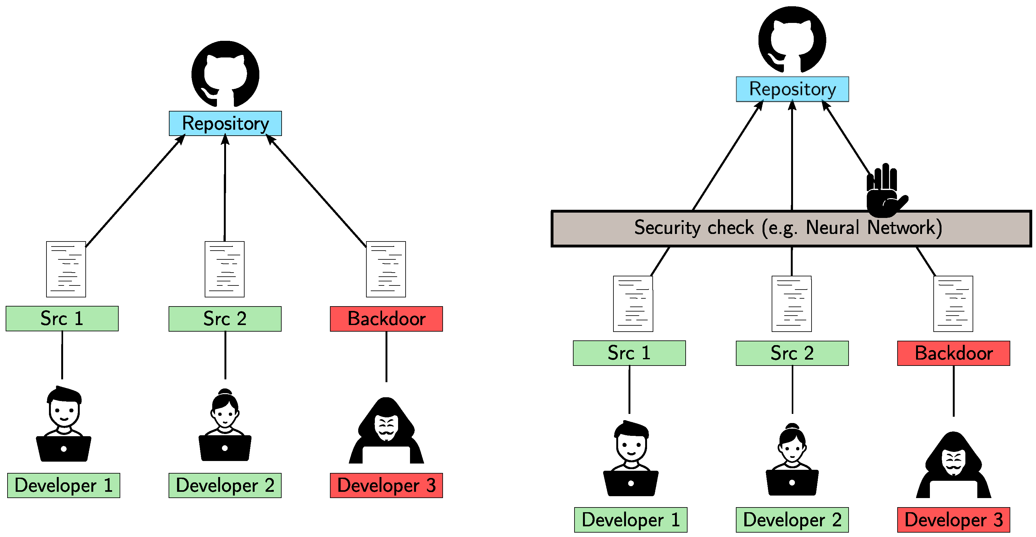
This study proposes to assess the robustness of a classification system by producing, with evolutionary techniques, program instances that mislead a system trained in the detection of software vulnerabilities. In other words, the goal is to synthesize vulnerable programs that will be classified as safe by the system, or vice versa. A possible application scenario is shown in
Figure 1, in which many developers make commits in a shared repository and one of them is malicious and wants to insert a backdoor. In an unsafe setting (left), the backdoor can be easily placed. In the setting reported in the right image, instead, a security check is installed, and the malicious code should be blocked. The goal of the attacker is thus to deceive the check and to push malicious code that is not detected. Given the described context, we define the following threat model, which is compliant with the approach presented by Papernot et al. [
25]:
The attacker can only act after the training phase;
The attacker only knows the output of the classifier, expressed as a probability;
The system is a black-box: the internal structure and the parameters are not visible;
The system acts as an oracle for the attacker, i.e., the attacker can ask for the classification of chosen instances;
The attacker has the goal of letting the system accept vulnerable code as safe;
The attacker can alter the input without affecting its original functionality.
The founding idea of this work is to design a method for adding some kind of noise to C functions, without altering their original functionality, to produce instances able to lead the network to a wrong classification decision. The input space is explored by means of an evolution strategy (ES) algorithm, which is an evolutionary technique that uses only mutations (and not crossover). We consider, as the fitness function, the numerical output of the network, and this insight allows us to efficiently explore the behavior of a neural classifier by leveraging an evolutionary pressure instead of randomly sampling its input space. We finally show how the proposed approaches can be effectively applied to fool a state-of-the-art network [
26] for vulnerability detection. All the experimental details that follow are given for C language, but the method and its light syntactical changes we operate on source code can be easily ported to other programming languages.
4. Experimental Settings
In this section, we present an overview of the methodology employed and the experimental setup. Specifically, we describe the model chosen, the evolutionary algorithm, and the mutation operators.
Neural Model Architecture
The model used as a benchmark to attack is a Convolutional Neural Network (CNN) proposed by Russell et al. [
26] for source code security assessment. The network architecture consists of multiple layers starting with an embedding layer that maps a complex and high-dimensional data structure into a simpler, lower-dimensional space that can be easily processed by a machine learning algorithm. This is followed by a 1D-convolutional layer which applies filters to capture local patterns in the input data; then, the pooling layer is employed to reduce the spatial dimensions of the input volume while retaining its depth. The model includes two fully connected hidden layers with dropout regularization and the output layer is the sigmoid activation function. An instance is classified as positive (vulnerable) if the output value exceeds 0.5 and as negative (non-vulnerable) otherwise.
Dataset Preprocessing
The dataset used is VDISC (
https://osf.io/d45bw/, accessed on July 2023) (Vulnerability Detection in Source Code of C and C++ languages), forming 1.27 million functions of source code extracted from open-source repositories. The dataset is divided into three portions, following an 80/10/10 ratio for training, validation, and testing, respectively. The network was trained using supervised learning to recognize vulnerabilities of type CWE-119 (
https://cwe.mitre.org/, accessed on July 2023), referring to the “Improper Restriction of Operations within the Bounds of a Memory Buffer”. The final test set used for this work consists of 1133 elements that are preprocessed to enable data parsing. During this preprocessing phase, the test set is cleaned of partial functions and syntax errors. For parsing the C language, the chosen parser is PycParser (
https://github.com/eliben/pycparser, accessed on July 2023), which supports the C99 language standard (ISO/IEC 9899), as well as some features from C11 and a few GCC extensions.
4.1. Evolution Strategy
An Evolution Strategy (ES) algorithm, specifically, the
variant [
27], is employed.
represents the number of parents selected in each iteration and
is the number of children generated by the parents.
is the version of ES where children replace parents, i.e., where the best
individuals of a population are mutated
times for composing the new generation. The fitness value during the evolution of individuals is measured as the output of the model to deceive and, dealing with binary classifiers, it is represented as a value that ranges from 0 to 1, where the values greater than
refer to the positive class, namely, to the instances that are classified as vulnerable. The goal is to invert the prediction of vulnerable functions and thus to let them be classified as safe, after having applied semantic-preserving mutations. This turns into lowering the probability below the threshold of
. Further, to ensure the attainment of significantly low probabilities, namely, probabilities that are far from the decision boundary, a stronger threshold of
is set to be reached. By applying the mutation operators and the selection mechanisms that will be detailed in
Section 4.2, the algorithm aims to optimize the fitness values of the individuals and reach the desired classification outcome.
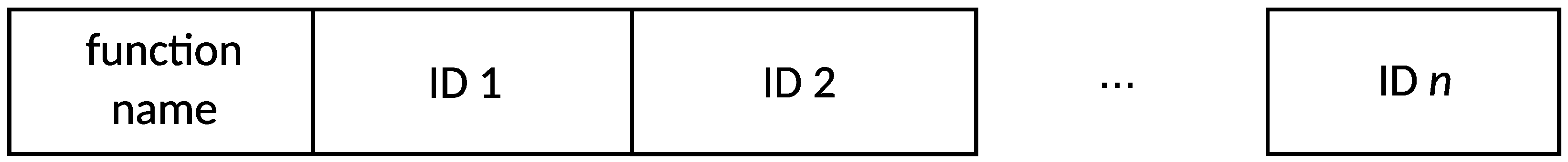
The genome refers to the complete set of genes that encode an individual’s traits or characteristics. In this context, the genome, shown in
Figure 2, is developed as a tuple where each slot contains an identifier of the analyzed individual. It provides a representation of the function (i.e., individual) to which mutations can be applied. By manipulating the genome, the ES algorithm can introduce random mutations and generate new variations of the original function. From any genome, the corresponding phenotype, that is, the corresponding source code individual, can be built from the original function identified by the unique name in the first element of the genome, by substituting in it all the identifiers according to the current name table described by the genome. To create a coherent initial population of individuals starting from a single individual of the dataset, each individual (i.e., function) with known ground truth (vulnerable) is parsed individually. For each individual of the dataset, a duplication strategy is employed, the individual (i.e., function) is duplicated, and the duplicate is given a different name identifier. By changing the name of the duplicated function, the population is enriched with variations while still retaining the original behavior of the function. The duplication, the renaming process, and the subsequent evolution and optimization through the ES algorithm add diversity to the population and enhance its representativeness. This step is repeated for each individual within the dataset, as shown in Algorithm 1. It details the phase of “create initial population”, and it is called by the ES algorithm, Algorithm 2.
| Algorithm 1: Create First Population |
| 1: loadDataset() |
▹ i.e., individuals
|
| 2: |
▹: initial population of each individual
|
| |
| 3:
| ▹ initialize empty array |
| 4: for all
do |
| 5:
|
| 6: copy(p) | ▹ duplicate individual |
| 7: Change the function identifier of |
|
8: Append to | ▹ population of the individual p |
| 9: Append to P | ▹ set of populations, one for each individual |
| 10: end for |
| 11: returnP |
| Algorithm 2: Evolution Strategy () |
| 1: | ▹ parents |
| 2: | ▹ children |
| |
| 3: createFirstPopulation() | ▹ see Algorithm 1 |
| 4: | ▹ initialize with a default value |
| 5: repeat |
| 6: for all do |
| 7: if or fitness() ≤fitness() then |
| 8: |
| 9: end if |
| 10:
end for |
| 11: the individuals in P with best fitness |
| 12: {} | ▹Join in () |
| 13: for all do |
| 14: for times do |
| 15: mutate(copy()) | ▹ mutation operator or |
| 16: end for |
| 17: end for |
| 18: until stopping criteria | ▹ Section 4.1 |
| 19: return Best |
The ES algorithm is applied by using two different mutation operators,
and
, which will be defined in
Section 4.2, and four different mutation probabilities, namely,
,
,
, and
. These mutation probabilities determine the probability of introducing changes in the individuals during each iteration of the ES algorithm, as detailed in Algorithm 2. Each experiment is repeated three times to guarantee the consistency of the data between runs. A total of 200 generations is chosen as the number of iterations for the ES algorithm relative to
, and 100 for
. Specifically, there is a disparity in the number of generations between
and
. In the case of
, employing 200 generations would lead to high computational time. Additionally, the set to be explored in
is not extensive. This selection guarantees a sufficiently broad range of iterations to adapt to the smallest mutation probability of 0.01 and allows it to eventually converge on the chosen threshold of
.
All the experiments are conducted on two Microsoft Azure virtual machines of the second generation. The first presents an x64 architecture, size standard F4s v2, vCPUs4, and RAM 8 GB. The second presents an x64 architecture, size standard D4ads v5, vCPUs4, and RAM 16 GB.
4.2. Mutation Operators
The proposed mutation operators are designed to introduce semantic-preserving modifications to existing functions, so as to alter the code of a program without altering its semantics, that is, the behavior of the program in terms of relation between input and output. In general, there exist many possible semantic-preserving transformations. Here, we consider two of them, one that is based on a consistent renaming of the variable identifiers, and the other one that relies on the introduction of dead code in the functions.
First operator
The mutation operator consists of modifying the identifiers within the source code of the functions so that, in each function F, each occurrence of the identifier IDi is consistently replaced with the same new identifier ID. To this end, two different vocabularies of words are used, and the algorithm can generate new variable names during the mutation process by selecting words from these vocabularies. They are meant to follow two different policies:
The first vocabulary is composed by
K generic English words (
https://github.com/dwyl/english-words, accessed on July 2023). It is used with the underlying idea of not bringing any domain-specific bias into the pool of possible identifiers. We will refer to this configuration as
.
The second, smaller, vocabulary is instead composed of ≈30 words or expressions that are somehow related to known vulnerabilities, shown in
Table A1 (in
Appendix A). We denote this experimental configuration with
.
Algorithm 3 shows the functioning of the first mutation operator
.
| Algorithm 3: First mutation operator |
| 1: input: individual p, genome | ▹ original genome |
| 2: output: individual p, genome | ▹ mutated genome |
| |
| 3: for all
do |
| 4: with probability do | ▹ mutation probability chosen |
| 5: IDfromVocab() | ▹ random identifier |
| 6: if then | ▹ check for consistency behavior |
| 7: | ▹ update genome with new identifier |
| 8: else |
| 9: while do |
| 10: IDfromVocab() |
| 11: end while |
| 12: |
| 13: end if |
| 14: updateIndiv1() |
| 15: done |
| 16: end for |
| 17: return
|
In the experiment, each run took approximately 21 h to complete. This indicates the time required for the ES algorithm to iterate through the specified number of generations, perform the fitness evaluations, and apply the mutations to the individuals in the population. For the experiment, instead, each run took approximately 10 h to complete.
With regard to the domain-specific set of words (
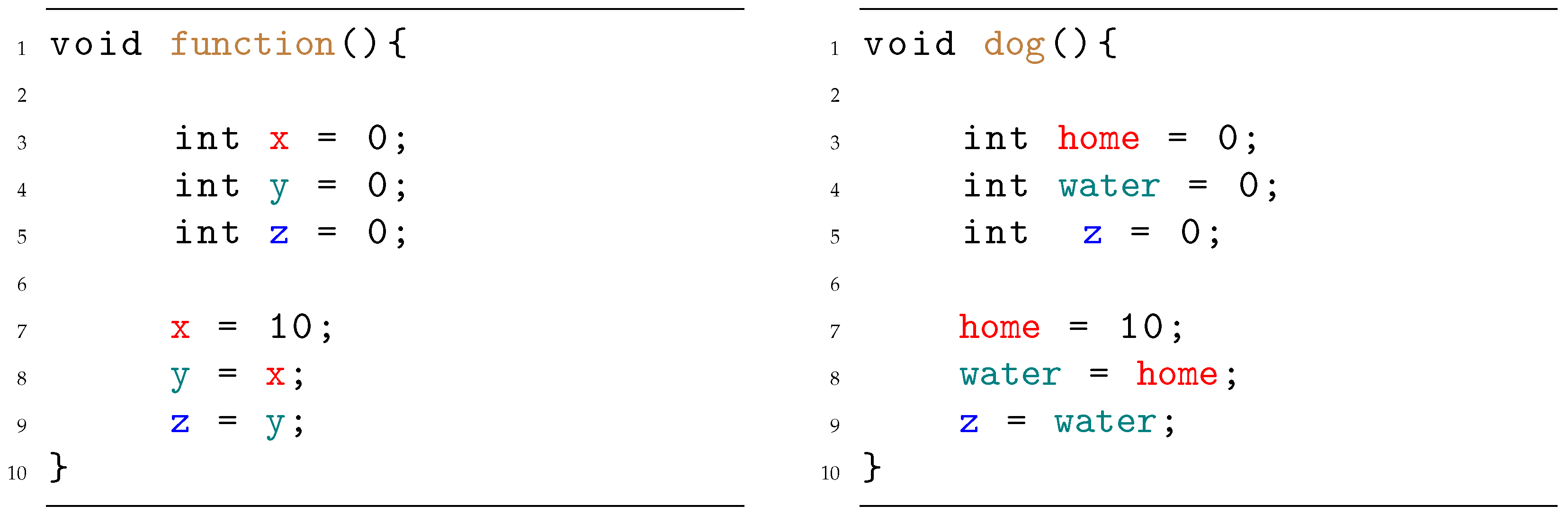
), in the context of black box attacks where explicit knowledge of the neural model is limited, an attempt is made to deceive the neural network using a limited vocabulary. This method aims to explore the possibility of influencing the model’s predictions by replacing words (identifiers) with others having different semantics. This choice comes because the model might misclassify code snippets containing trigger words that might recall vulnerability names. A simplified example of input and output is shown in
Figure 3 and
Figure 4.
Second operator
The second mutation operator consists of injecting non-executable code into functions as part of the mutation process. The purpose of this mutation is to simulate potential vulnerabilities and generate new variations of the functions for analysis. By injecting non-executable code, this mutation introduces a certain level of unpredictability and randomness into the model. By analyzing its behavior on the mutated functions, the algorithm can reveal potential weaknesses and evaluate their impact on the vulnerability detection process.
The addition of dead code is performed before the closing bracket of the function, with conditional statements whose conditions always result in a negative outcome, and thus whose content is never executed. This kind of modification ensures that the behavior of the function remains unchanged. This approach is taken to prevent any unintended modifications to the function’s functionality. The primary objective involves incorporating code that somehow deceives the classifier. These instructions or instruction sequences are designed to introduce noise in the classifier, which consequently can be confusing during its decision-making process. This kind of mutation operator is tested in two experimental variants:
Injection of generic sequences of instruction that are not supposed to be related to any vulnerability. This variant is referred to as .
Injection of sequences of instructions that if executed would introduce a flaw. We will refer to this variant as .
Algorithm 4 shows the functioning of the second mutation operator
. Notice that all the algorithms presented in this section make use of some auxiliary functions that are summarised and defined in Algorithm 5.
| Algorithm 4: Second mutation operator |
| 1: input: individual p, genome | ▹ original genome |
| 2: output: individual p, genome | ▹ mutated genome |
| |
| 3: with probability do | ▹ mutation probability chosen |
| 4: deadCodeFromVocab() | ▹ extract dead code |
| 5: Append c to | ▹ update genome |
| 6: updateIndiv2() |
| 7: done |
| 8: return
|
| Algorithm 5: Auxiliary functions |
- 1:
procedure copy(p) - 2:
- 3:
return - 4:
end procedure - 5:
- 6:
proceduredeadCodeFromVocab() - 7:
return a random item from a library of dead code snippets - 8:
end procedure - 9:
- 10:
procedure fitness(p) - 11:
return as fitness the classifier’s output value with input p - 12:
end procedure - 13:
- 14:
procedure IDFromVocab() - 15:
return a random identifier from a vocabulary - 16:
end procedure - 17:
- 18:
procedure loadDataset() - 19:
Load a set D of C-language functions - 20:
return D - 21:
end procedure - 22:
- 23:
procedure updateIndiv1() - 24:
Modify the source code p according to the identifiers in the genome - 25:
end procedure - 26:
- 27:
procedure updateIndiv2() - 28:
Add the code block c to the original code p before the last curly bracket - 29:
end procedure
|
For both
and
, each run took approximately 22 h to complete. The first experiment of this second mutation
refers to the injection of non-vulnerable code samples to try to force the classifier to reverse the prediction from true to false. In order to further assess the robustness of the neural model classification system, a decision was made to conduct additional testing (
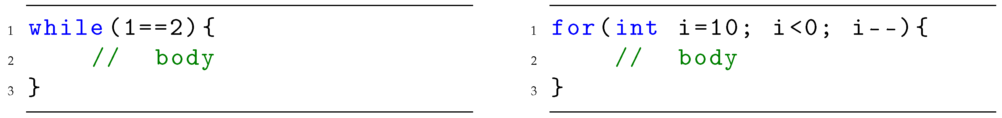
) involving the injection of non-executable “vulnerable code”. The objective of this test was to determine if some non-executable block code containing vulnerable code could still deceive the model. Code that is inside a loop or conditional statement that is never executed is referred to as “dead code” with no effect at run time because it is unreachable.
Figure 5 shows examples of C code that will never be executed.
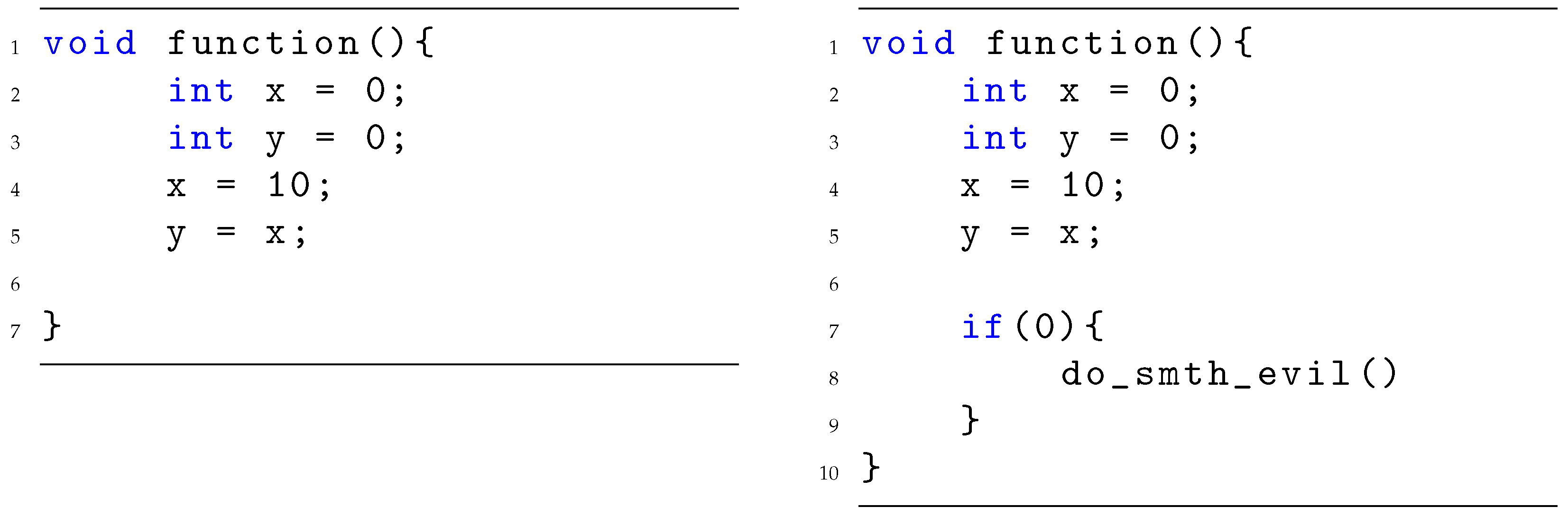
Each mutation is applied with a given probability. To introduce the injected code, two libraries are used: one containing vulnerable code options and the other containing non-vulnerable code options. The code for injection is already inserted in “dead blocks”. From these lists, a code snippet is randomly selected for injection. This selection process adds an element of randomness to the mutation, allowing for the exploration of different code variations that can simulate potential vulnerabilities or non-vulnerable scenarios. A simplified example of input and output is shown in
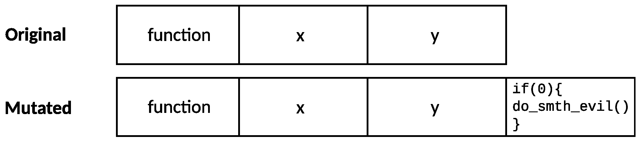
Figure 6. The genome structure is correspondingly expanded, so that trailing genes encode the blocks to be injected in the phenotype, as can be seen in
Figure 7.
5. Results
This section analyzes and shows the obtained results. For compactness, only the results of the lowest and highest tested mutation probabilities are included. Notice however that the other tested probabilities exhibit similar trends.
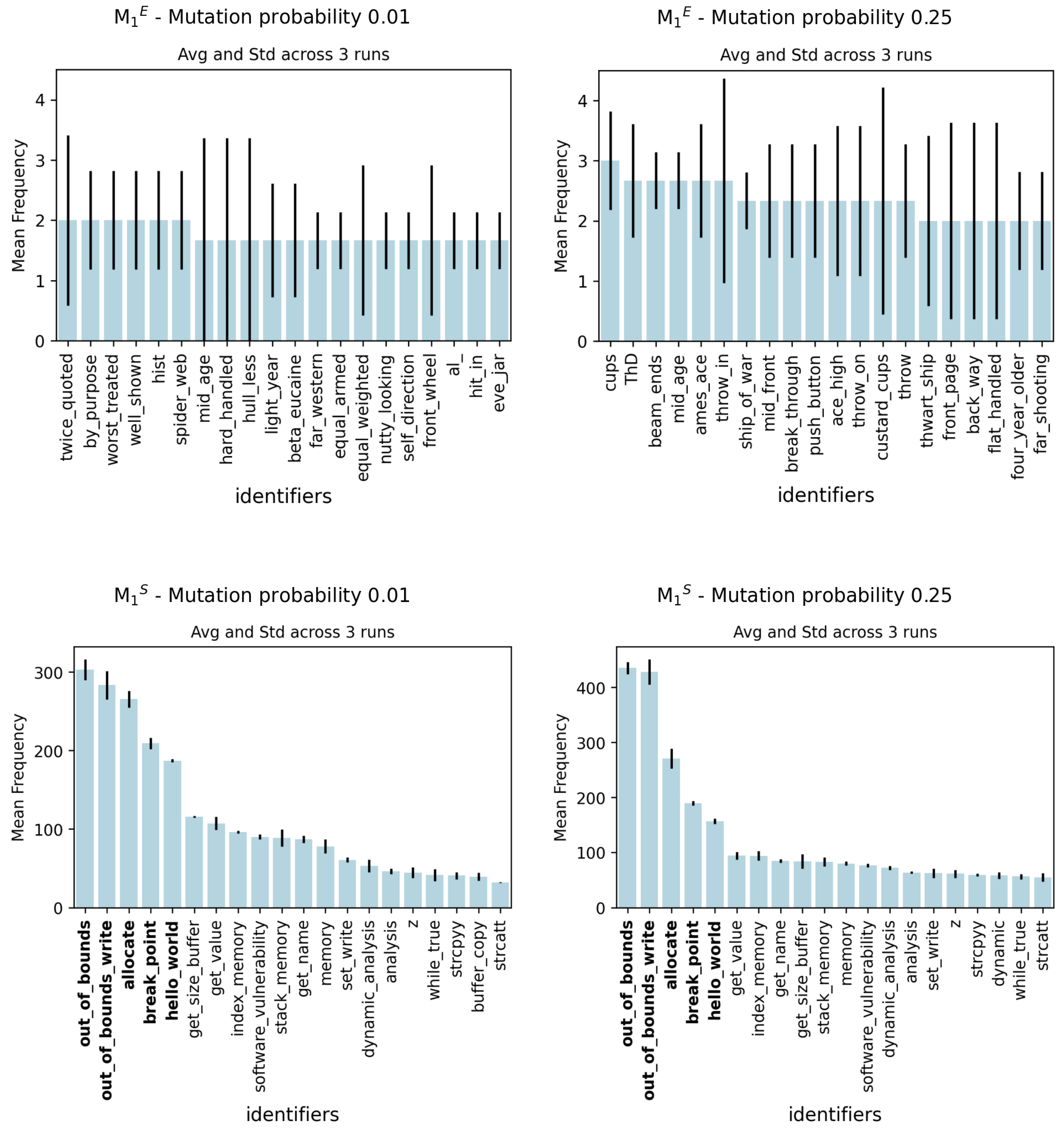
As an initial step in the analysis of the results, word analysis on experiments was conducted to determine if any specific patterns could potentially deceive the model.
Figure 8 shows the most frequent words for
and
experiment. The most frequent words represent a count that is determined by analyzing the genome of each individual which succeeded in deceiving the classifier. We remark that each genome is created in such a way that contains the structure of an individual uniquely referring to the identifiers, as shown in
Figure 2. Therefore, in cases where an identifier appears multiple times within an individual, it is counted as a single occurrence.
The results of
, show a significant variation across the three runs. One can observe that with an increase in the mutation probability, there is a slight decrease in variation as indicated by the standard deviations depicted in the graphs. Analyzing the data in
Figure 8, there is a great divergence of standard deviation between the different runs; this should be for the large size of the vocabulary
E in combination with the individuals mutating with a very low probability. Due to this, the ES might not have explored the entire set of words comprehensively. Despite the challenge posed by the large set of words, the ES algorithm was still able to discover names that effectively deceive the model. We see in
Figure 8 that vocabulary
E, used in the
configuration, also uses composite identifiers formed by combining two separate words already present in the generic English vocabulary we adopted.
For , this simple experiment shows how easy the possibility of misleading the neural network is even with a restricted set of words, thereby highlighting the model’s high sensitivity to even minor variations. The results demonstrate no substantial variations across the three runs for each mutation probability. In particular, the words out_of_bounds and out_of_bound_write always have the highest frequencies, together with three other words highlighted in bold in the figure.
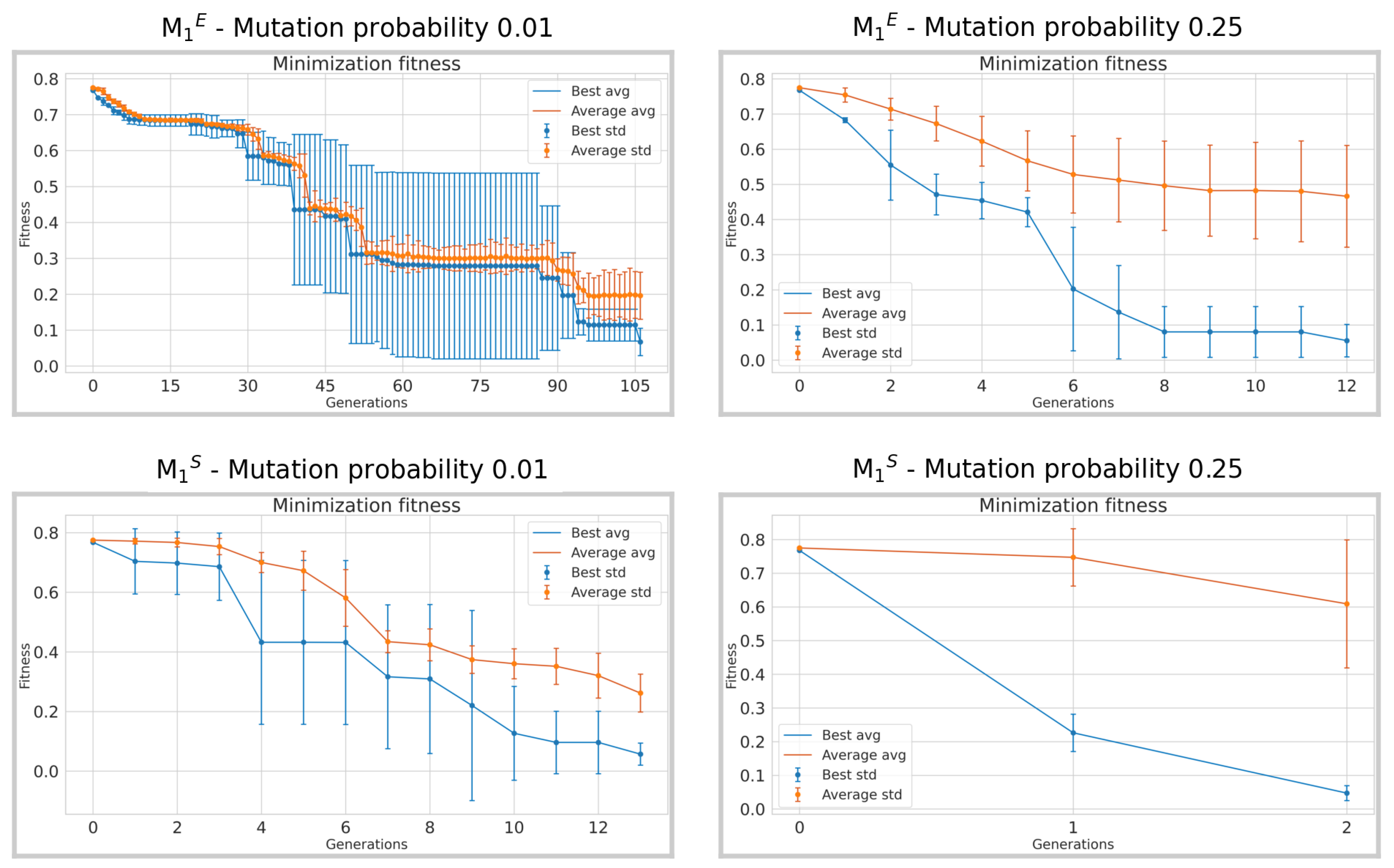
When examining the comparison between individuals with the lowest probability of 0.01 and the highest probability of 0.25, in both experimental conditions denoted as
and
in
Figure 9 and
Figure 10, a notable decrease in the number of generations needed for convergence is observed. Approximately 100 and 11 generations were needed for experiments in
to reach the chosen convergence threshold of 0.1, considering a mutation probability of 0.01. In particular, it only requires two generations in
and 9 in
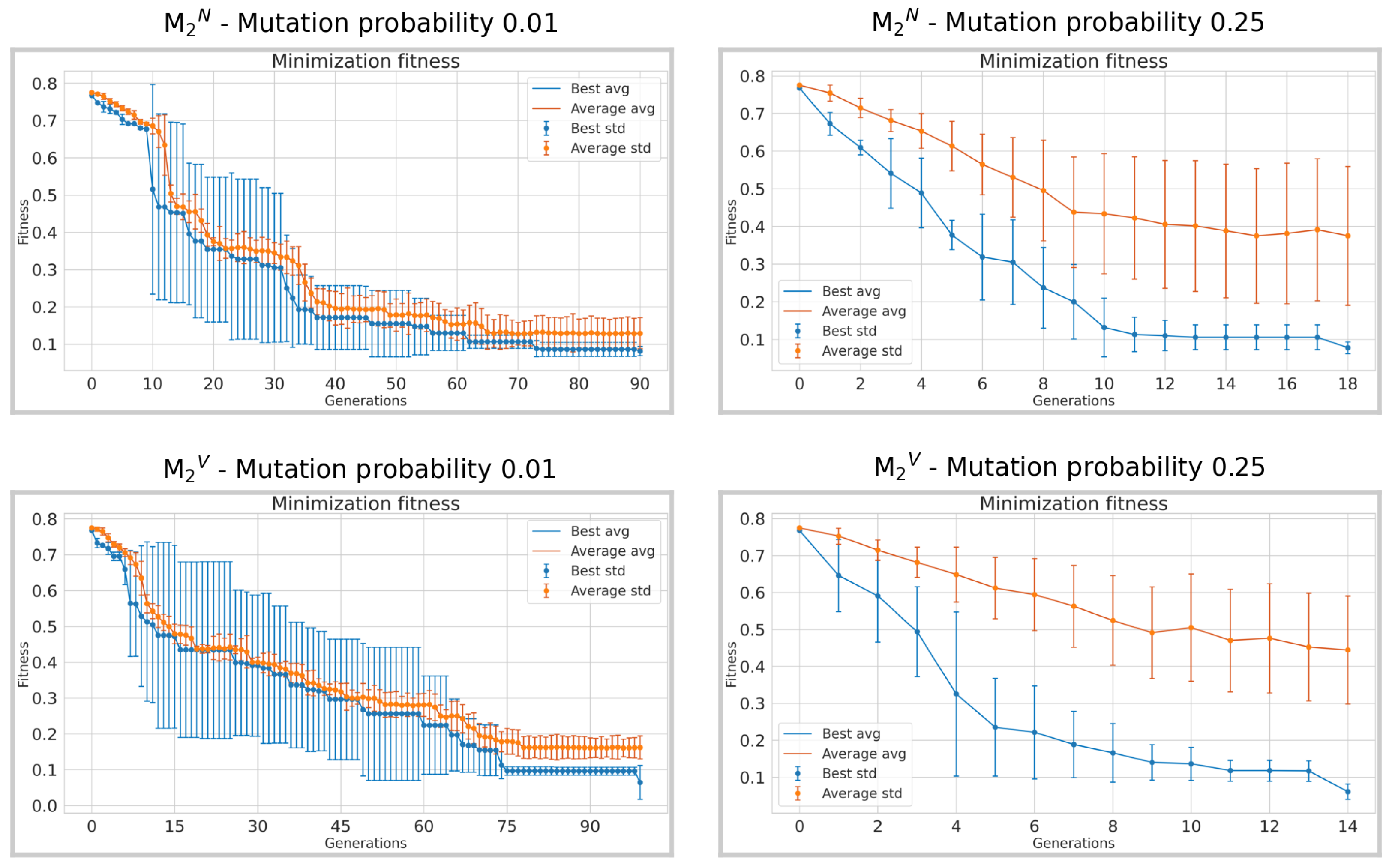
for individuals with a probability of 0.25. This indicates a much faster convergence rate with higher mutation probabilities especially in the restricted set of words; this represents an expected result. A similar trend occurs in the experiments
, where about 65 generations in
and 75 in
are required for the lowest mutation probability, and about 13 for the highest mutation probability.
Table 1 reports the results of the classifier; specifically, the outcomes across the three runs are nearly similar, with minimal standard deviation across three runs, so we decided to report the count from the run that achieved the worst results. In both experiments
and
, the model was consistently deceived with a high probability ranging from 90% to 100%. We remark that the goal is to reverse the classification (from True to False). Specifically, in the first mutation, the true positive rates reach zero at the highest percentage value of 25% for
and at the lowest percentage value of 1% for
. This indicates that all labels have been reversed in these cases. In the second mutation operation,
, the model demonstrates improved performance at higher levels of mutation probability. Upon analyzing the results, we observed that as the mutation rate increases from 10% to 25%, there is a reduction in the number of true positives and only a minimal change in the number of false negatives. In the case of the lowest mutation probability of 1%, the results show that the model was deceived in more than 90% of the cases, even in the worst run.
6. Conclusions and Further Directions
This work shows how a state-of-the-art neural classifier trained to look for vulnerabilities in source code can be deceived by automatically changing any given malicious input code while still preserving its semantics. The method maps the input source code to a genome representation and the genome is evolved according to a process that consistently mutates the identifiers and injects code without affecting the original behavior of the snippet.
The method has been successfully applied by operating on the test part of the same dataset which was used to train the classifier. This is particularly relevant since it means that the system has been confused without moving the input to a completely new and possibly misunderstood space, but staying close to the original test space, where during its development the classifier showed good accuracy.
By examining which identifiers were successful in our attack, we discovered that among a restricted set of words (in ), composed by mixing words semantically related to software security topics and words unrelated to them, the system was shown to be particularly sensitive to security-related terms. This could point to undesired biases developed during the training phase, possibly due to a strong presence of these words in specific subclasses of the dataset’s instances.
Future steps could be mainly devoted to two goals. First, different source code mutation operators could be used during the evolutionary search for adversarial variations of input instances. Secondly, a stronger and finer assessment of the biases of the classifier emerging from the statistics gathered during the evolution of adversarial examples should be developed. This would be key in understanding and improving how the trained classifiers operate internally.
Author Contributions
Conceptualization, V.M., C.F. and M.S.; methodology, C.F. and M.S.; software, V.M.; investigation, V.M.; data curation, V.M.; analysis, V.M., C.F. and M.S.; visualization, V.M. and M.S.; writing—original draft preparation, V.M., C.F. and M.S.; writing—review and editing, C.F. and M.S. All authors have read and agreed to the published version of the manuscript.
Funding
This research received no external funding.
Institutional Review Board Statement
Not applicable.
Data Availability Statement
Conflicts of Interest
The authors declare no conflict of interest.
Appendix A
Table A1.
The table reports the vocabulary used in the experiment.
Table A1.
The table reports the vocabulary used in the experiment.
| allocate | get_size_buffer | software_vulnerability |
| analysis | get_value | stack |
| break_point | hello_world | stack_memory |
| buffer | index | strcpyy |
| buffer_copy | index_buffer | strcatt |
| buffer_kernel | index_memory | while_false |
| buffer_overflow | kernel | while_true |
| dynamic | memory | write |
| dynamic_analysis | out_of_bounds | x |
| flag | out_of_bounds_write | y |
| get_name | set_write | z |
References
- Akhtar, N.; Mian, A.S. Threat of Adversarial Attacks on Deep Learning in Computer Vision: A Survey. IEEE Access 2018, 6, 14410–14430. [Google Scholar] [CrossRef]
- Ferretti, C.; Saletta, M. Naturalness in Source Code Summarization. How Significant is it? In Proceedings of the 31st IEEE/ACM International Conference on Program Comprehension, ICPC 2023, Melbourne, Australia, 15–16 May 2023; pp. 125–134. [Google Scholar]
- Allamanis, M.; Barr, E.T.; Devanbu, P.T.; Sutton, C. A Survey of Machine Learning for Big Code and Naturalness. ACM Comput. Surv. 2018, 51, 81:1–81:37. [Google Scholar] [CrossRef]
- Le, T.H.M.; Chen, H.; Babar, M.A. Deep Learning for Source Code Modeling and Generation: Models, Applications, and Challenges. ACM Comput. Surv. 2021, 53, 62:1–62:38. [Google Scholar] [CrossRef]
- Del Carpio, A.F.; Angarita, L.B. Trends in Software Engineering Processes using Deep Learning: A Systematic Literature Review. In Proceedings of the 46th Euromicro Conference on Software Engineering and Advanced Applications (SEAA), Portoroz, Slovenia, 26–28 August 2020; pp. 445–454. [Google Scholar]
- Idika, N.; Mathur, A.P. A survey of malware detection techniques. Purdue Univ. 2007, 48, 32–46. [Google Scholar]
- Liu, B.; Shi, L.; Cai, Z.; Li, M. Software vulnerability discovery techniques: A survey. In Proceedings of the 2012 Fourth International Conference on MULTIMEDIA Information Networking and Security, Nanjing, China, 2–4 November 2012; pp. 152–156. [Google Scholar]
- Yamaguchi, F.; Lindner, F.F.; Rieck, K. Vulnerability Extrapolation: Assisted Discovery of Vulnerabilities Using Machine Learning. In Proceedings of the 5th USENIX Workshop on Offensive Technologies, WOOT’11, San Francisco, CA, USA, 8 August 2011; pp. 118–127. [Google Scholar]
- Fang, Y.; Han, S.; Huang, C.; Wu, R. TAP: A static analysis model for PHP vulnerabilities based on token and deep learning technology. PLoS ONE 2019, 14, e0225196. [Google Scholar] [CrossRef] [PubMed]
- Li, Z.; Zou, D.; Xu, S.; Ou, X.; Jin, H.; Wang, S.; Deng, Z.; Zhong, Y. VulDeePecker: A Deep Learning-Based System for Vulnerability Detection. In Proceedings of the 25th Annual Network and Distributed System Security Symposium, NDSS, San Diego, CA, USA, 24–27 February 2019. [Google Scholar]
- Li, Z.; Zou, D.; Xu, S.; Jin, H.; Zhu, Y.; Chen, Z. SySeVR: A Framework for Using Deep Learning to Detect Software Vulnerabilities. IEEE Trans. Dependable Secur. Comput. 2022, 19, 2244–2258. [Google Scholar] [CrossRef]
- Chakraborty, S.; Krishna, R.; Ding, Y.; Ray, B. Deep Learning Based Vulnerability Detection: Are We There Yet? IEEE Trans. Softw. Eng. 2022, 48, 3280–3296. [Google Scholar] [CrossRef]
- Kotsiantis, S.B. Supervised Machine Learning: A Review of Classification Techniques. In Emerging Artificial Intelligence Applications in Computer Engineering—Real Word AI Systems with Applications in eHealth, HCI, Information Retrieval and Pervasive Technologies; Frontiers in Artificial Intelligence and Applications; IOS Press: Amsterdam, The Netherlands, 2007; Volume 160, pp. 3–24. [Google Scholar]
- Karimi, H.; Derr, T. Decision Boundaries of Deep Neural Networks. In Proceedings of the 21st IEEE International Conference on Machine Learning and Applications ICMLA, Paradise Island, The Bahamas, 12–14 December 2022; pp. 1085–1092. [Google Scholar]
- He, W.; Li, B.; Song, D. Decision Boundary Analysis of Adversarial Examples. In Proceedings of the 6th International Conference on Learning Representations, ICLR, Vancouver, BC, Canada, 30 April–3 May 2018. [Google Scholar]
- Su, J.; Vargas, D.V.; Sakurai, K. One Pixel Attack for Fooling Deep Neural Networks. IEEE Trans. Evol. Comput. 2019, 23, 828–841. [Google Scholar] [CrossRef]
- Goodfellow, I.J.; Shlens, J.; Szegedy, C. Explaining and Harnessing Adversarial Examples. In Proceedings of the 3rd International Conference on Learning Representations, ICLR, San Diego, CA, USA, 7–9 May 2015. [Google Scholar]
- Yefet, N.; Alon, U.; Yahav, E. Adversarial examples for models of code. Proc. ACM Program. Lang. 2020, 4, 162:1–162:30. [Google Scholar] [CrossRef]
- Zhang, H.; Li, Z.; Li, G.; Ma, L.; Liu, Y.; Jin, Z. Generating Adversarial Examples for Holding Robustness of Source Code Processing Models. In Proceedings of the 34th AAAI Conference on Artificial Intelligence, AAAI, New York, NY, USA, 7–12 February 2020; pp. 1169–1176. [Google Scholar]
- Quiring, E.; Maier, A.; Rieck, K. Misleading Authorship Attribution of Source Code using Adversarial Learning. In Proceedings of the 28th USENIX Security Symposium, Santa Clara, CA, USA, 14–16 August 2019; pp. 479–496. [Google Scholar]
- Ferretti, C.; Saletta, M. Deceiving neural source code classifiers: Finding adversarial examples with grammatical evolution. In Proceedings of the GECCO ’21: Genetic and Evolutionary Computation Conference, Lille, France, 10–14 July 2021; pp. 1889–1897. [Google Scholar]
- Saletta, M.; Ferretti, C. A Grammar-based Evolutionary Approach for Assessing Deep Neural Source Code Classifiers. In Proceedings of the IEEE Congress on Evolutionary Computation, CEC, Padua, Italy, 18–23 July 2022; pp. 1–8. [Google Scholar]
- Saletta, M.; Ferretti, C. Towards the evolutionary assessment of neural transformers trained on source code. In Proceedings of the GECCO ’22: Genetic and Evolutionary Computation Conference, Boston, MA, USA, 9–13 July 2022; pp. 1770–1778. [Google Scholar]
- Ferretti, C.; Saletta, M. Do Neural Transformers Learn Human-Defined Concepts? An Extensive Study in Source Code Processing Domain. Algorithms 2022, 15, 449. [Google Scholar] [CrossRef]
- Papernot, N.; McDaniel, P.; Sinha, A.; Wellman, M.P. SoK: Security and Privacy in Machine Learning. In Proceedings of the IEEE European Symposium on Security and Privacy (EuroS&P), London, UK, 24–26 April 2018; pp. 399–414. [Google Scholar]
- Russell, R.; Kim, L.; Hamilton, L.; Lazovich, T.; Harer, J.; Ozdemir, O.; Ellingwood, P.; McConley, M. Automated vulnerability detection in source code using deep representation learning. In Proceedings of the 17th IEEE International Conference on Machine Learning and Applications (ICMLA), Orlando, FL, USA, 17–20 December 2018; pp. 757–762. [Google Scholar]
- Luke, S. Essentials of Metaheuristics, 2nd ed.; Lulu: Morrisville, NC, USA, 2013; Available online: http://cs.gmu.edu/~sean/book/metaheuristics/ (accessed on 1 July 2023).
Figure 1.
Possible attack scenario.
Figure 1.
Possible attack scenario.
Figure 2.
Genome structure. The first position refers to the function name, while the others (ID1, ID2, …, IDn) are the identifiers, that is, the names assigned to entities such as variables, functions, and structures.
Figure 2.
Genome structure. The first position refers to the function name, while the others (ID1, ID2, …, IDn) are the identifiers, that is, the names assigned to entities such as variables, functions, and structures.
Figure 3.
Application of the mutation operator. The code on the left represents the original function, while the code on the right represents the same code after the mutation, where some of the identifiers have been changed to random English words.
Figure 3.
Application of the mutation operator. The code on the left represents the original function, while the code on the right represents the same code after the mutation, where some of the identifiers have been changed to random English words.
Figure 4.
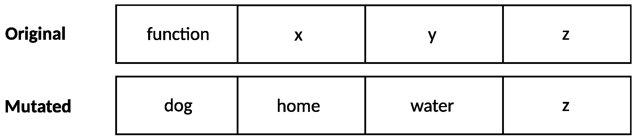
Genome of the function presented in
Figure 3. The model takes a function as its input; the corresponding genome is obtained through AST manipulation.
Figure 4.
Genome of the function presented in
Figure 3. The model takes a function as its input; the corresponding genome is obtained through AST manipulation.
Figure 5.
Dead code examples. Both the bodies inside the while (left) and for blocks (right) cannot be executed, since the conditions are never satisfied.
Figure 5.
Dead code examples. Both the bodies inside the while (left) and for blocks (right) cannot be executed, since the conditions are never satisfied.
Figure 6.
Application of the mutation operator. The code on the left represents the original function, while the code on the right represents the same code after the mutation, where the code is expanded with the injection.
Figure 6.
Application of the mutation operator. The code on the left represents the original function, while the code on the right represents the same code after the mutation, where the code is expanded with the injection.
Figure 7.
Genome of the function presented in
Figure 6. After the mutation, the injected code remains unchanged and represents an immutable part of the genome; this is because since blocks of code are not executable, it is possible to insert multiple equal blocks without affecting the functionality or execution of the code.
Figure 8.
Frequency of top 20 words for and experiment that have successfully deceived the network. The plots report the mean and standard deviation across 3 runs for the lowest 0.01 and the highest 0.25 mutation probabilities.
Figure 8.
Frequency of top 20 words for and experiment that have successfully deceived the network. The plots report the mean and standard deviation across 3 runs for the lowest 0.01 and the highest 0.25 mutation probabilities.
Figure 9.
Average fitness obtained across 3 runs for the lowest 0.01 and the highest 0.25 mutation probabilities of the experiments. Vertical bars represent the standard deviation and the orange curves represent the average fitness of the population at each generation, while the blue curves represent the fitness of the best individual at each generation. The x-axis is truncated at the point the algorithm achieves convergence.
Figure 10.
Average fitness obtained across 3 runs for the lowest 0.01 and the highest 0.25 mutation probabilities of the experiments. Vertical bars represent the standard deviation, the orange curves represent the average fitness of the population at each generation, and the blue curves represent the fitness of the best individual at each generation. The x-axis is truncated at the point where the algorithm achieves convergence.
Table 1.
Final results of the worst run for each experimental configuration.
Table 1.
Final results of the worst run for each experimental configuration.
| Experiment | Mutation Probability | Not Inverted | Inverted | % Success |
|---|
| 0.01 | 44 | 1089 | 96.1% |
| | 0.1 | 2 | 1131 | 99.8% |
| | 0.15 | 1 | 1132 | 99.9% |
| | 0.25 | 0 | 1133 | 100% |
| 0.01 | 0 | 1133 | 100% |
| | 0.1 | 3 | 1130 | 99.7% |
| | 0.15 | 1 | 1132 | 99.9% |
| | 0.25 | 1 | 1132 | 99.9% |
| 0.01 | 113 | 1020 | 90% |
| | 0.1 | 6 | 1127 | 99.4% |
| | 0.15 | 5 | 1128 | 99.5% |
| | 0.25 | 5 | 1128 | 99.5% |
| 0.01 | 113 | 1020 | 90% |
| | 0.1 | 7 | 1126 | 99.3% |
| | 0.15 | 6 | 1127 | 99.4% |
| | 0.25 | 4 | 1129 | 99.6% |
| Disclaimer/Publisher’s Note: The statements, opinions and data contained in all publications are solely those of the individual author(s) and contributor(s) and not of MDPI and/or the editor(s). MDPI and/or the editor(s) disclaim responsibility for any injury to people or property resulting from any ideas, methods, instructions or products referred to in the content. |
© 2023 by the authors. Licensee MDPI, Basel, Switzerland. This article is an open access article distributed under the terms and conditions of the Creative Commons Attribution (CC BY) license (https://creativecommons.org/licenses/by/4.0/).


