A Review on Data-Driven Condition Monitoring of Industrial Equipment

Abstract

This paper presents an up-to-date review of data-driven condition monitoring of industrial equipment with the focus on three commonly used equipment: motors, pumps, and bearings. Firstly, the general framework of data-driven condition monitoring is discussed and the utilized mathematical and statistical approaches are introduced. The utilized techniques in recent literature are discussed. Then, fault detection, diagnosis, and prognosis on the three types of equipment are highlighted using a variety of popular shallow and deep learning models. Applications of these techniques in recent literature are summarized. Finally, some potential future challenges and research directions are presented.

1. Introduction

With the continuous improvement of the industrialization level, the design and manufacturing technologies of the equipment have also advanced swiftly, making the equipment’s safety and reliability increasingly significant [1]. Equipment in operation is constantly exposed to various environmental forces (such as cutting forces, friction, ambient temperature, and vibration), and is susceptible to wear and tear, rusting of parts, deterioration of components, and other problems, leading to frequent abnormalities in the equipment, resulting in a gradual decline in its efficiency and life, and even catastrophic failures. To address these issues, condition monitoring of equipment has attracted tremendous research attention to ensure the safety and reliability of production [2,3,4,5,6,7]. Based on online monitoring of time-series data, the failure process can be separated into two stages for most of the equipment, as depicted in Figure 1. The first phase is the normal operating phase, which begins with the installation and commissioning of the system and ends with the appearance of abnormalities. During this phase, the monitored data is relatively steady and has no discernible pattern of change. The second stage is the progression from the appearance of anomalies to the degradation and eventual failure of the equipment. If the abnormalities discovered in this phase lead directly to equipment failure, a fault detection and diagnostic model is constructed based on the monitored data to determine the fault type, severity, and location. If the data observed during this phase reveals a tendency of degradation that is not severe enough to impede the normal operation of the equipment, a model can be constructed to predict the failure and estimate the remaining useful life of the equipment based on the degradation trend. There are three steps in equipment condition monitoring: (1). data collection; (2). data processing; and (3). Fault detection, diagnosis, and prediction. Data collection refers to the real-time monitoring of parameters or signals relevant to the performance state of the equipment using various types of sensors, and the aggregation of the collected data. Data processing refers to the pre-processing of signals or data obtained by sensors, including noise reduction, reconstruction, and feature extraction. Features include time-domain features, frequency-domain features, time-frequency-domain features, and features autonomously learnt by deep learning models. Lastly, for the detected deviations from normal operation, intelligent fault diagnosis algorithms are used to determine the specific fault type of the equipment, and for equipment exhibiting signs of degradation or failure, prediction algorithms are used to predict the future trend of the equipment’s performance state and its remaining useful life.

In general, the method to condition monitoring has undergone three stages of development, with the first relying on manual monitoring and diagnosis by specialized engineers. The second development stage produces the data-driven condition monitoring based on the continuous growth of sensor technology, more and more novel sensors are installed or integrated in the equipment to gather real-time monitoring information of the equipment, and a large number of signal analysis techniques are suggested and implemented in the monitoring sector, realizing the contemporary fault diagnosis technology with fault mechanism, sensor monitoring, and signal analysis as the co-main technologies. The most renowned of these are mathematics and statistics-based techniques, including Fourier Transform (FT), Wavelet Transform (WT), and Empirical Modal Decomposition (EMD) [8,9,10]. The third stage of development is artificial intelligence-based condition monitoring, where artificial intelligence techniques, mainly represented by machine learning, have been quickly developed. In the field of intelligent condition monitoring of equipment, machine learning algorithms are used in conjunction with techniques such as fault mechanism and signal analysis. The most common approaches are shallow learning algorithms represented by artificial neural networks (ANN), support vector machines (SVM) and extreme learning machines (ELM) [11,12,13], and deep learning algorithms represented by deep belief networks (DBN), convolutional neural networks (CNN) and recurrent neural networks (RNN) [14,15,16]. Motors, pumps, and bearings, as key components of industrial systems and applications, are essential equipment in the contemporary industrial sector. These essential pieces of equipment must work with reliability and safety [17,18,19,20]. Therefore, the main objective of this paper is to review the condition monitoring of equipment, particularly for motors, pumps, and bearings, based on the data-driven methods.

The remaining parts of the paper are organized as follows. Data-driven condition monitoring approaches for motors, pumps and bearings are presented in Section 2. Different data processing methods and their applications in the monitoring of industrial equipment are discussed. Then, data-driven fault detection techniques and their applications to industrial equipment are presented. Finally, Section 3 discusses challenges and future trends.

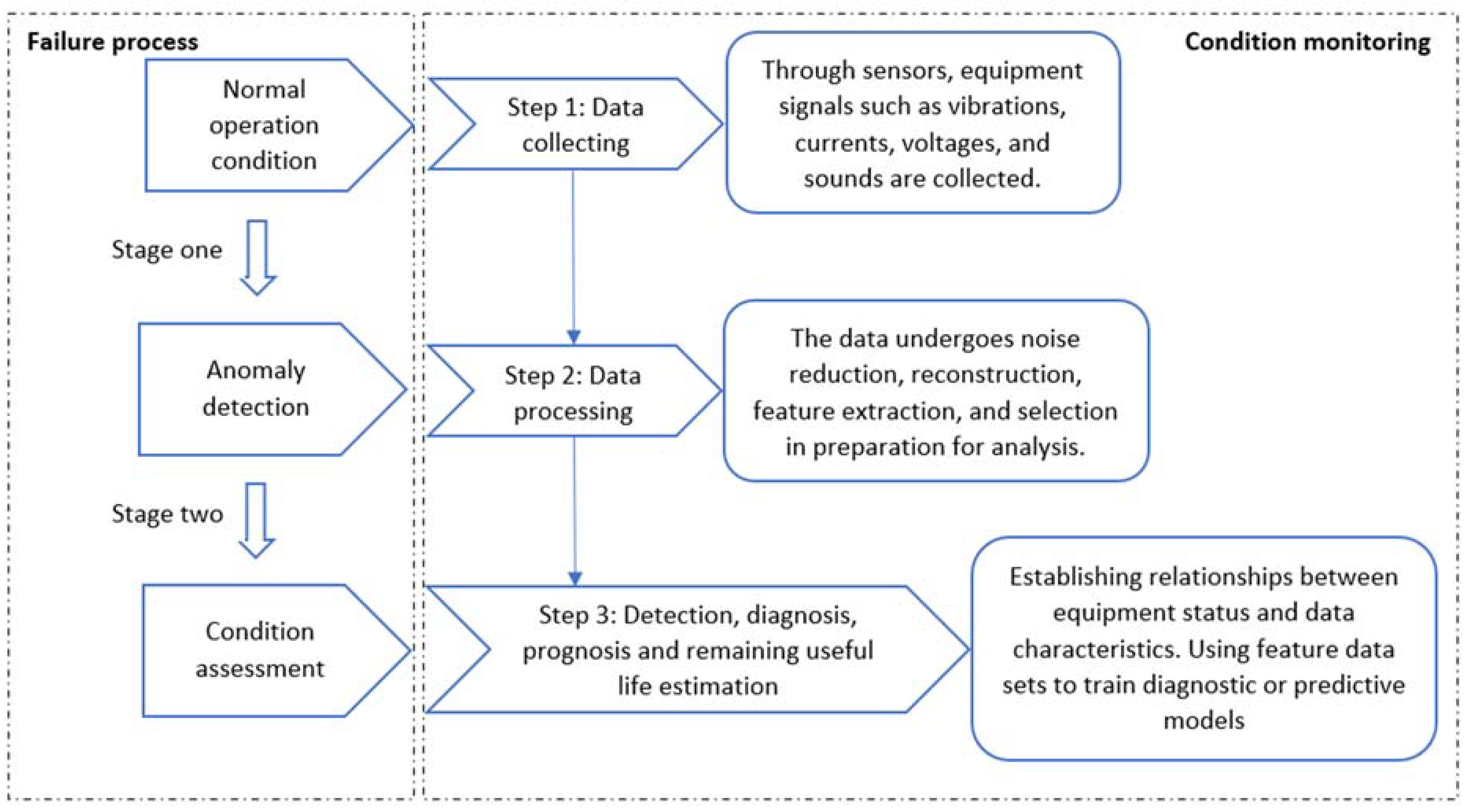
2. Data-Driven Condition Monitoring of Industrial Equipment

Data-driven condition monitoring technology relies on various sources and types of monitoring data collected during the operation of the equipment and employs various data mining techniques to extract the useful information implied therein, thereby enabling condition monitoring and fault diagnosis of the equipment [21,22,23]. As mentioned previously, the deployment of this technology consists of three steps: data collection; data processing; and fault detection, diagnosis and prediction. The methods and applications of data processing and condition monitoring and prediction are reviewed next in this section.

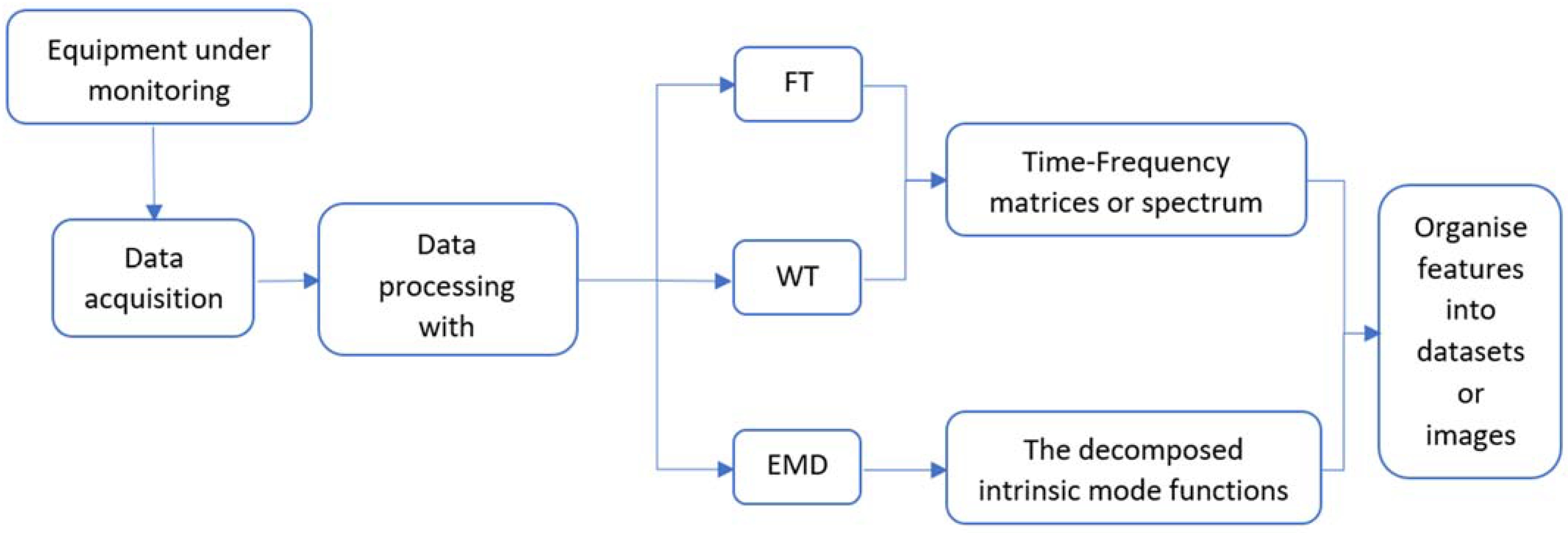
2.1. Data Processing Methods

Feature extraction and feature selection are the most critical parts of data processing techniques. Features extraction is the process of obtaining sensitive features from the original signal that effectively highlight variations between the various operation conditions of the equipment. Time-domain feature extraction, frequency-domain feature extraction, and time-frequency feature extraction are the primary feature extraction methods, with the kind and physical relevance of the derived characteristics dictating which approach is utilized. The method for selecting a sensitive, highly differentiated, and moderately dimensional collection of features from the initial defect feature set is known as feature selection [24,25].

Fourier Transform, Wavelet Transform, and Empirical Model Decomposition are the primary approaches. Figure 2 shows a simple flow chart for applying these three techniques.

2.1.1. The Fourier Transform Approach

The FT approach can be used to extract time-varying signal information in the frequency domain and compare it to the characteristics of the normal state for condition monitoring. Although the Fourier transform links the time and frequency domain properties of a signal, allowing for analysis and diagnosis of the signal state in the frequency domain, it is impossible to establish the time of occurrence of any frequency in the signal spectrum in the time domain. Frequently, the test signal at the time of failure coincides to an abrupt shift in frequency. Based on the Fourier transform, the Short-time Fourier transform (STFT) method is presented to analyze the frequency information of a time-varying signal at a certain time interval or instant.

The STFT for any signal $\mathrm{x}\left(\mathrm{t}\right)$ is defined as:

$${\mathrm{S}}_{\mathrm{x}}\left(\mathrm{t}, \mathsf{\omega }\right)=\underset{-\infty }{\overset{+\infty }{{\displaystyle \int }}}\left[\mathrm{x}\left(\mathsf{\tau }\right)\mathrm{g}\left(\mathrm{t}-\mathsf{\tau }\right)\right]{\mathrm{e}}^{-\mathrm{j}\mathsf{\omega }\mathsf{\tau }}\mathrm{d}\mathsf{\tau }$$

(1)

where $\mathsf{\tau }$ is the time shift parameter, $\mathrm{x}\left(\mathsf{\tau }\right)$ is the time-domain signal, and $\mathrm{g}\left(\mathrm{t} - \mathsf{\tau }\right)$ represent the time window, which represents a function that is constantly equal to 0 or quickly converges to 0 outside a finite interval, in which the centre is located at time $\mathsf{\tau }$. Although STFT is capable of handling non-stationary signals, it is better suited for the analysis of quasi-stationary signals, particularly long-period quasi-stationary signals, but not for the analysis of local time-frequency characteristics of non-stationary signals, as it is a Fourier transform on local intervals. Currently, STFT is mostly utilized for equipment condition monitoring.

STFT has been successfully applied to equipment signal analysis and feature extraction in previous research because its benefits in dealing with non-stationary random signals [26,27,28,29,30]. Therefore, extensive study has been conducted on condition monitoring strategies that combine this method with other methodologies. For example, in [31], the discrete Fourier transform (DFT) is used to analyse the voltage signal waveform of the Brushless DC motor to detect if a fault has occurred and to determine the number of turns shorted. Then, frequency domain analysis of the integrated voltage characteristic waveform is performed by STFT to determine the index of the faulty phase. Finally, an independent adaptive neuro-fuzzy inference system (ANFIS) is used to implement detection and diagnosis of stator interturn short circuit faults. Aimer et al. [32] analyzed the current signal of an induction motor with a broken rotor bar fault using STFT. On the produced time-frequency diagram of the current signal, several harmonics were noted, and the sideband frequencies were computed, allowing for the detection and diagnosis of the fault. In [33], STFT is used to analyse the vibration signals of rolling element bearing under different states and obtained the time-frequency distribution (TFD) characterizing the local faults. Then, the TFDs of nine different bearing faults (e.g., inner race fault, ball fault and outer race fault) were extracted, clustered, and identified by non-negative matrix decomposition (NMF). The results show that the fault identification accuracy of the method can reach 99.3%, which is much higher than the accuracy of 75.8% of ANN. He et al. [34] converted the raw bearing time-domain acoustic emission sensor signals into frequency domain signals by STFT, which resulted in a spectrum matrix. The sub-modes generated from the spectrum matrix are then used to train the LSMSTAR network model for bearing fault diagnosis, which achieves accurate classification of various bearing faults under different operating conditions. Similarly, Zhao et al. [35] used the STFT to decompose multiple eigenmode functions (IMFs) of the plunger pump’s vibration signal obtained by complete empirical mode decomposition (CEMD). After that, the time-frequency matrices of the signals in different operating states of the plunger pump were obtained, and the time-frequency entropy of each state was calculated once to extract the features. The obtained feature matrices are then dimensionally reduced by using principal component analysis (PCA). Finally, the processed signal features are used to train a support vector machine (SVM) classifier for the diagnosis of swash plate and rotor wear faults. In addition, STFT has also been applied to signal dimensional conversion. For example, Chao et al. [36] converted the one-dimensional vibration signal of an axial piston pump into a two-dimensional spectrogram by STFT, and effectively improved the accuracy of the STFT spectrogram feature map by a denoising method, which was used as the input to a LeNet-5 convolutional neural network to effectively improve the ability to identify cavitation conditions in noisy environments. Tao et al. [37] also used STFT to transform the 1D time-domain vibration signals of bearings into 2D time-frequency maps, and the multiple time-frequency maps obtained by adjusting the length of the STFT window were used as input to a classification generative adversarial network (CatGAN), which was trained to obtain a CatGAN model for diagnosing inner race and outer race faults.

The corresponding references for the FT methods reviewed in this section are summarised in

Table 1. Motor condition monitoring using Fourier transform.

References	Application	Type of Equipment	Signal	Fault Type
[26]	Fault diagnosis	Servo motor	Current signal	Axis misalignment (right and left axis with different amplitude)
[30]	Fault diagnosis	Induction motor	Current signal	Rotor and bearing fault
[31]	Fault diagnosis	Brushless DC motor	Voltage signal	Stator interturn short circuits
[32]	Fault diagnosis	Induction motor	Current signal	Broken rotor bar fault (One or several bars broken)
[38]	Fault diagnosis	Asynchronous motor	Vibration signal	Built-in rotor imbalance, stator winding faults, built-in faulted bearing, built-in bowed rotor, built-in broken rotor bars, voltage imbalance and single phasing

,

Table 2. Pump condition monitoring using Fourier transform.

References	Application	Type of Equipment	Signal	Fault Type
[27]	Feature extraction	Centrifugal pump	Vibration signal	Cavitation
[35]	Fault diagnosis	Plunger pump	Vibration signal	Swash plate wear and rotor wear
[36]	Fault diagnosis	Axial piston pumps	Vibration signal	Cavitation (different severity)
[39]	Fault detection	Centrifugal pump	Vibration signal	Cavitation
[40]	Fault detection	Centrifugal pump	Vibration signal	Cracks and imbalances in impellers of varying degrees are simulated manually by making port dramas and hammer blows. (Impeller damage due to corrosion in the fluid and external solids materials)
[41]	Fault detection	Gear pump	Vibration signal	Abrupt changes in the behaviour caused by cavitation
[42]	Fault classification	Motor pump	Vibration signal	Misalignment unbalance rubbing accelerometer fault

and

Table 3. Bearing condition monitoring using Fourier transform.

References	Application	Type of Equipment	Signal	Fault Type
[28]	Feature extraction	Rolling bearing	Vibration signal	Ball, inner race, and outer race faults
[29]	Fault diagnosis	Rolling bearing	Vibration signal	Roller, inner race, and outer race faults
[33]	Feature extraction	Rolling bearing	Vibration signal	9 kinds of bearings with various faults, i.e., inner race fault, ball fault and outer race fault with 3 diameters status
[34]	Feature extraction	Rolling bearing	Vibration signal	Inner race, outer race, cage, and ball faults
[37]	Fault diagnosis	Rolling bearing	Vibration signal	Ball, inner race, and outer race faults

.

2.1.2. The Wavelet Transform Approach

The WT approach can be used to decompose the signal at multiple scales and obtain local features in the time-frequency domain through a series of wavelet basis functions and is one of the most important tools in the time-frequency analysis of non-stationary signals.

Let $\mathsf{\Psi }\left(\mathrm{t}\right)\in {\mathrm{L}}^2\left(\mathrm{R}\right)$ (where ${\mathrm{L}}^2\left(\mathrm{R}\right)$ is the square integrable real number space), then the Fourier transform of $\mathsf{\Psi }\left(\mathrm{t}\right)$ is when the following admissibility condition is met:

$${\mathrm{C}}_{\mathsf{\Psi }}=\underset{-\mathrm{\infty }}{\overset{+\mathrm{\infty }}{{\displaystyle \int }}}\frac{|\hat{\mathsf{\Psi }}(\mathsf{\omega }){|}^2}{|\mathsf{\omega }|}\mathrm{d}\mathsf{\omega }<+\mathrm{\infty }$$

(2)

where $\hat{\mathsf{\Psi }}(\mathsf{\omega }=0)=0$.

$\mathsf{\Psi }\left(\mathrm{t}\right)$ represents the mother function, which can be shifted, stretched, or compressed to give a wavelet sequence (sub wavelet) after the transformation as follow.

$${\mathsf{\Psi }}_{\mathrm{a},\mathrm{b}}\left(\mathrm{t}\right)=\frac{1}{\sqrt{\mathrm{a}}}\mathsf{\Psi }\left(\frac{\mathrm{t}-\mathrm{b}}{\mathrm{a}}\right) \mathrm{a},\mathrm{b}\in \mathrm{R}, \mathrm{a}\ne 0$$

(3)

where the role of $\mathrm{a}$ is to scale the mother function $\mathsf{\Psi }\left(\mathrm{t}\right)$, known as the scale factor, and the role of $\mathrm{b}$ is to temporally localize the mother wavelet, known as the shift factor.

The WT inherits and expands upon the concept of STFT localization, resolving the issue that the window size in STFT does not change with frequency by providing a time-frequency window that fluctuates with frequency. Therefore, the WT can be utilized for condition monitoring by analyzing changes in the signal’s mutation value and frequency structure, as well as by utilizing the WT to denoise and extract waveform information from the signal [30,43,44]. In [45], Siddiqui and Giri used WT to decompose the stator current signal of an induction motor and extract low frequency features to represent the fault information. All the useful information of the fault is obtained by superimposing the waveforms, distinguishing the healthy and faulty states of the motor, and achieving the detection of broken rotor bar faults. In addition, many variants of the WT have also been successfully applied to equipment condition monitoring. These include continuous wavelet transform (CWT) [46,47], discrete wavelet transforms (DWT) [48,49,50,51], and empirical wavelet transform (EWT) [52]. CWT is often used to extract and analyse the wavelet features of a signal. Muralidharan and Sugumaran [53] used CWT to analyze the Monoblock centrifugal pump vibration signals and obtained feature sets consisting of different wavelets and used them as inputs to a classifier to obtain the maximum fault identification capability for the system. Finally, the diagnosis of single and hybrid faults of the pump bearing was achieved by combining the decision tree approach. In addition, CWT is also used to convert time series signals into time-frequency images. For example, Xu et al. [54] converted the bearing vibration signal into a time-frequency image by a series of CWT and used it as the input to a convolutional neural network. After training the network with multilayer pooling, unique features corresponding to faults can be captured from the original CWT images, which are then used as inputs to the gcForest model for fault classification. The results show that the hybrid model achieves high accuracy in detecting and diagnosing multiple bearing faults for datasets of different sizes. Tang et al. [55] used CWT to convert time series of vibration, pressure, and sound signals of hydraulic axial piston pumps under different operating conditions into two-dimensional time-frequency images and developed a convolutional neural network fault diagnosis model based on an adaptive learning rate strategy for each signal. The results showed that the average accuracy of fault diagnosis using different signals was 97.33%, 99.48% and 98.77%. In [56], Kamiel et al. used the DWT with multi-resolution analysis (MRA) to perform a five-level wavelet decomposition of the original pump vibration signal to obtain the low and high frequency features of the signal. Subsequently, a principal component analysis (PCA) model was constructed from the low frequency features obtained under normal operating conditions to accurately detect single and multiple faults (cavitation, impeller faults and combinations of cavitation and impeller faults) in centrifugal pumps, and analysis of the principal component scores and load maps enabled fault identification. Al Tobi et al. [57] also used DWT to perform a six-level decomposition of the vibration signal of a centrifugal pump, extracting 60 approximate and detailed features for different mother wavelet functions, and applied them to train a multilayer perceptron-based backpropagation neural network and support vector machine model. It was found that with the use of rbio1.5 mother wavelet decomposition, not only fewer feature parameters could be obtained, but also the accuracy of the fault detection and diagnosis model could be achieved at 100%. In [58], the EWT was used to extract the modes of the bearing vibration signals of the motor and their corresponding envelope spectra, and the corresponding fault eigenfrequencies obtained were used to implement fault detection. By comparing and analyzing the effectiveness of EWT with empirical mode decomposition (EMD) using simulated and real data, it was found that EWT has better performance in weak feature detection and composite fault detection, while EMD can only extract one temporal frequency of the fault feature frequencies and cannot detect faults under strong noise interference. Eren et al. [59] applied EWT to analyze the Fourier spectrum segments of motor vibration signals extracted by Fast Fourier Transform (FFT). The time domain contribution of the corresponding spectral bands was also obtained by inverse Fourier transform and finally the root mean square value of the time domain signal was calculated to achieve motor bearing fault detection.

The corresponding references for the WT methods reviewed in this section are summarized in

Table 4. Motor condition monitoring using wavelet transform.

References	Application	Type of Equipment	Signal	Fault Type
[30]	Fault diagnosis	Induction motor	Current signal	Rotor and bearing fault
[43]	Fault detection	Induction motor	Current signal	Air gap eccentricity fault
[45]	Fault detection	Induction motor	Current signal	Broken rotor bar fault
[48]	Fault diagnosis	Induction motor	Vibration signal	Rotor and bearing faults
[49]	Fault diagnosis	Permanent magnet synchronous motor	Current signal	Broken magnet and eccentricity faults
[59]	Fault detection	Induction motor	Vibration signal	Bearing fault
[60]	Fault diagnosis	Permanent magnet synchronous motor	Current, voltage and speed signal	Static and dynamic eccentricity fault

,

Table 5. Pump condition monitoring using wavelet transform.

References	Application	Type of Equipment	Signal	Fault Type
[51]	Fault feature identification	Reactor coolant pump	Vibration signal	Rotor crack faults
[52]	Feature extraction	Hydraulic pump	Vibration signal	Loose slipper fault
[53]	Feature extraction and fault diagnosis	Monoblock centrifugal pump	Vibration signal	Bearing fault, impeller defect, bearing, and impeller defect together and cavitation
[55]	Fault diagnosis	Hydraulic pump	Vibration, pressure, and sound signal	Swash plate wear, loose slipper, slipper wear, and central spring wear
[56]	Feature extraction	Hydraulic pump	Vibration signal	Slipper fault
[57]	Fault diagnosis	Centrifugal pump	Vibration signal	Five mechanical faults (bearing, misalignment, unbalance, impeller, and looseness), and a hydraulic fault (cavitation)
[61]	Fault diagnosis	Centrifugal pump	Vibration signal	Suction flow blockages and casing cavitation
[62]	Fault diagnosis	Hydraulic pump	Vibration signal	Slipper loosing and Valve plate wear fault

and

Table 6. Bearing condition monitoring using wavelet transform.

References	Application	Type of Equipment	Signal	Fault Type
[44]	Fault diagnosis	Rolling bearings	Vibration signal	Roller, inner race, and outer race faults
[46]	Fault detection	Rolling bearings	Vibration signal	Bearing faults
[47]	Fault diagnosis	Rolling bearings	Vibration signal	Inner race and outer race faults
[50]	Fault detection and diagnosis	Rolling bearings	Voltage and current signals	Partially and heavily damaged bearing fault
[54]	Fault diagnosis	Rolling bearings	Vibration signal	Ball, inner race, and outer race faults
[58]	Fault detection	Rolling bearings	Vibration signal	Motor bearing with outer race weak defect (spalling fault in the outer race of generator bearing in this wind turbine)
[63]	Fault diagnosis	Rolling bearing	Vibration signal	Inner race, outer race, and roller faults
[64]	Fault diagnosis	Spindle bearing	Vibration signal	Inner race, outer race, and ball faults

below.

2.1.3. The Empirical Model Decomposition Approach

The EMD approach is an adaptive decomposition method for non-stationary signals proposed by Huang et al. [10]. in 1998. Using an iterative screening process, the approach decomposes the original non-stationary signal with poor performance and contaminants into a sequence of new, improved sequence of signals representing the oscillatory part of the original signal, which is also called the intrinsic mode functions (IMF). By layer-by-layer deconstructing the components of different feature scales in the signal, it is easier to extract the distinctive information parameters of the condition monitoring signal, which has gained significant attention in equipment fault diagnosis. The steps of EMD are as follows:

(a)

After calculating all local extremes of the original signal $\mathrm{x}\left(\mathrm{t}\right)$, a cubic spline function is used to link all local maxima as the upper envelope ${\mathrm{e}}_{+}\left(\mathrm{t}\right)$, followed by a cubic spline function to connect all local minima as the lower envelope ${\mathrm{e}}_{-}\left(\mathrm{t}\right)$. The mean envelope $\mathrm{e}\left(\mathrm{t}\right)$ is then determined between the upper and lower envelopes. Next, subtract $\mathrm{e}\left(\mathrm{t}\right)$ from the original signal $\mathrm{x}\left(\mathrm{t}\right)$ to obtain a new signal ${\mathrm{m}}_1\left(\mathrm{t}\right)$.

$${\mathrm{m}}_1\left(\mathrm{t}\right)=\mathrm{x}\left(\mathrm{t}\right) - \mathrm{e}\left(\mathrm{t}\right)$$

(4)

(b)

If ${\mathrm{m}}_1\left(\mathrm{t}\right)$ satisfies the IMF criteria [65], it is recorded as ${\mathrm{c}}_1\left(\mathrm{t}\right)$ as the first order IMF. If not, continue step a using ${\mathrm{m}}_1\left(\mathrm{t}\right)$ as the original signal $\mathrm{x}\left(\mathrm{t}\right)$ until, after $\mathrm{k}$ times computations, ${\mathrm{m}}_{\mathrm{k}}\left(\mathrm{t}\right)$ meets the IMF criteria then ${\mathrm{m}}_{\mathrm{k}}\left(\mathrm{t}\right)$ is the desired first order IMF.

$${\mathrm{c}}_1\left(\mathrm{t}\right){=\mathrm{m}}_{\mathrm{k}}\left(\mathrm{t}\right)$$

(5)

(c)

Subtract ${\mathrm{c}}_1\left(\mathrm{t}\right)$ from the original signal $\mathrm{x}\left(\mathrm{t}\right)$ to obtain the new signal ${\mathrm{r}}_1\left(\mathrm{t}\right)$ as:

$${\mathrm{r}}_1\left(\mathrm{t}\right)=\mathrm{x}\left(\mathrm{t}\right){ - \mathrm{c}}_1\left(\mathrm{t}\right)$$

(6)

As ${\mathrm{r}}_1\left(\mathrm{t}\right)$ still contains some IMF, it is treated as a new original input signal and steps a–c are repeated to find the $\mathrm{n}$ components until the iterative process stops when ${\mathrm{r}}_{\mathrm{n}}$ is a monotonic function or a constant.

$$\{\begin{array}{c}{\mathrm{r}}_1\left(\mathrm{t}\right)=\mathrm{x}\left(\mathrm{t}\right){-\mathrm{c}}_1\left(\mathrm{t}\right)\\ {\mathrm{r}}_2\left(\mathrm{t}\right){=\mathrm{r}}_1\left(\mathrm{t}\right){-\mathrm{c}}_2\left(\mathrm{t}\right)\\ ⋮\\ {\mathrm{r}}_{\mathrm{n}}\left(\mathrm{t}\right){=\mathrm{r}}_{\mathrm{n}-1}\left(\mathrm{t}\right){-\mathrm{c}}_{\mathrm{n}}\left(\mathrm{t}\right)\end{array}$$

(7)

where ${\mathrm{c}}_1\left(\mathrm{t}\right){, \mathrm{c}}_2\left(\mathrm{t}\right), \cdots {, \mathrm{c}}_{\mathrm{n}}\left(\mathrm{t}\right)$ represent the information of the signal from high to low frequencies. This completes the entire EMD process, where the original signal $\mathrm{x}$ is split into several components and a sum of residual functions.

$$\mathrm{x}\left(\mathrm{t}\right)={\displaystyle \sum }_{\mathrm{i}=1}^{\mathrm{n}}{\mathrm{c}}_{\mathrm{i}}\left(\mathrm{t}\right){+\mathrm{r}}_{\mathrm{n}}\left(\mathrm{t}\right)$$

(8)

The various order components characterize the different frequency components of the signal and the residual function represents the average trend of the signal.

EMD is also a popular method for time-frequency domain signal analysis. Compared to wavelet transform techniques, it overcomes the problem of non-adaptive basis functions and eliminates the requirement for pre-determined basis functions, making it more adaptive to non-linear and non-stationary signals. This has won the approach a great deal of attention in the field of equipment condition monitoring [66,67,68,69,70,71,72,73]. In [74], the envelope analysis of the IMF obtained by EMD decomposition of the vibration signal of the hydraulic pump casing was carried out to derive the envelope spectrum of the first three IMFs containing the main information about the fault and used to implement fault diagnosis. The experiments show that the method can effectively diagnose the slipper loosing, swashplate wearing and valve plate wearing faults of hydraulic pump. In [75], EMD is used to extract the IMFs of the different frequency bands of the induction motor current. The dominating IMF is obtained for the analysis of motor faults by decomposing the current signals in different motor operating modes. The results show that the diagnosis of broken rotor bars faults in induction motors can be accurately done by evaluating the variation of the amplitude of the IMF oscillation, under varied loads. Sadeghi et al. [76], used EMD to decompose the stator current of an induction motor into multiple IMFs with specific frequency bands, and the IMF in the first row with the fastest response to the fault was used for the detection of motor stator faults. Subsequently, to distinguish between motor current fluctuations caused by normal operation and those caused by fault conditions, the instantaneous frequency (IF) variation of the IMFs is used as a criterion for fault detection. Through different simulations and experiments, this method outperforms the WT and FT methods overall in terms of efficiency and accuracy of fault detection. However, as the acquired equipment signals are typically combined with noise or unknown intermittent signals, this may lead to model confusion when utilizing EMD for signal decomposition due to repeated jumps in the local extremes in a short time interval. To tackle this difficulty, improved EMD algorithms have been brought into the field of equipment condition monitoring, such as ensemble EMD (EEMD) [77,78,79,80,81] and complete ensemble EMD (CEEMD) [82,83]. In [84], the collected aviation hydraulic pump pressure signals were decomposed into several IMFs using EEMD to reflect the fault characteristics in the time, frequency, and time-frequency domains to define the severity of the faults. Using PCA to scale down the defect characteristics, a support vector regression (SVR) model was then developed to predict the remaining life of the pump. It is demonstrated that the multi-domain fault characteristics retrieved by EEMD can more precisely reflect the severity of the loose piston defect and the remaining useful life of pump can be estimated by the SVR model. Zhao et al. [85] propose a new method for extracting fault features. Initially, the fault vibration signals of the inner ring, outer ring, and rolling element of the bearing are decomposed into IMFs with different physical significance by EEMD. Then, the IMFs with the highest correlation coefficients are chosen to characterize the original fault signals using the correlation coefficient analysis method. The obtained IMF multi-scale fuzzy entropy values are then used to generate a feature vector for the training and construction of the SVM classifier. Several experiments demonstrate that the approach can accurately detect and diagnose the type and severity of bearing faults under varying motor loads and bearing fault severity levels. CEEMD was suggested in [86] to increase algorithm efficiency and reduce computing costs, and it has been successfully used to condition monitoring. In [87], Delgado-Arredondo et al. used CEEMD to decompose microphone-recorded induction motor acoustic sound signals. The CEEMD was utilized to temporally decompose motor sound signals acquired under normal and fault operating conditions, and the corresponding spectrum of IMFs obtained by time-frequency distribution of Gabor (TFDG) was used to select specific IMFs containing fault information for fault diagnosis. It is shown that the diagnosis of unbalance condition, bearing faults, and broken rotor bar defects can be accomplished by comparing the spectra of IMFs of sound signals under normal and faulty operating conditions, and that the validity of the results can be verified by analyzing vibration signals. A defect feature extraction optimization approach is proposed in [88] for CEEMD. A genetic algorithm is used to optimize the white noise amplitude of the CEEMD so that the decomposition produces the least mean value of mutual information between the IMFs, thereby suppressing the model mixing phenomena. The method is used to the diagnosis of bearing faults, and the results indicate that the optimized method can adaptively analyze diverse signals and provide more sensitive diagnostic results than the empirically chosen white noise approach.

The corresponding references for the EMD methods reviewed in this section are summarized in

Table 7. Motor condition monitoring using empirical model decomposition.

References	Application	Type of Equipment	Signal	Fault Type
[66]	Fault diagnosis	Synchronous motor	Current signal	Broken damper bars with different asymmetry
[71]	Fault detection	Induction motor	Current signal	Rotor bar fault
[75]	Fault diagnosis	Induction motor	Current signal	Broken rotor bars (one or several bars)
[76]	Fault detection	Induction motor	Current signal	Stator short circuit faults (stator winding fault)
[87]	Fault diagnosis	Induction motor	Sound and vibration signal	Unbalance condition, bearing faults and broken rotor bars
[89]	Fault detection and diagnosis	Induction motor	Current signal	Bearing fault (Outer race and inner race)
[90]	Fault diagnosis	Permanent magnet Brushless DC motor	Current and vibration signal	Stator and rotor faults

,

Table 8. Pump condition monitoring using empirical model decomposition.

References	Application	Type of Equipment	Signal	Fault Type
[35]	Fault diagnosis	Plunger pump	Vibration signal	Swash plate wear and rotor wear
[67]	Fault diagnosis	Hydraulic piston pump	Discharge pressure signal	Swashplate wear fault, piston shoe loose fault, and piston shoe wear fault
[68]	Fault diagnosis	Airborne fuel pump	Vibration and pressure signal	Blade damage, diffusion tube damage, leakage, diffusion tube impeller rub, and bearing wear
[72]	Feature extraction	Nuclear main pump	Vibration signal	Rolling bearing fault
[74]	Fault diagnosis	Hydraulic pump	Vibration signal	Slipper losing fault, swashplate wearing faut and valve plate wearing fault
[77]	Fault diagnosis	Gear pump	Vibration signal	Tooth face wear, cavitation, oil pollution, and wear of internal surface sleeve
[81]	Fault prognosis	Reactor coolant pump	Shaft seal leakage flow	Seal leakage fault
[82]	Fault diagnosis	Vacuum pump	Acoustic emission signal	Overload fault (an overload fault was realized by changing the suction load conditions and extracting the atmosphere at full power is considered an overload fault and extracting the pressure vessel through the aperture is considered normal.)
[84]	Fault detection	Aviation piston pump	Discharge pressure signal	loose piston defect
[91]	Fault diagnosis	Hydraulic pump	Vibration signal	Single slipper wear, single slipper loose, and center spring wear faults
[92]	Fault diagnosis	Reciprocating pump	Vibration signal	Piston wear, bearing wear, and valve disc wear faults

and

Table 9. Bearing condition monitoring using empirical model decomposition.

References	Application	Type of Equipment	Signal	Fault Type
[69]	Fault diagnosis	Rolling bearing	Vibration signal	Outer race, inner race, and ball faults
[70]	Fault diagnosis	Rolling bearing	Vibration signal	Outer race, inner race, and ball faults
[73]	Fault detection and diagnosis	Bearing in main coolant pump and feed water pump	Vibration signal	Inner race, outer race, and ball faults
[78]	Fault diagnosis	Locomotive roller bearing	Vibration signal	Slight rub fault in the outer race Serious flaking fault in the outer race, slight rub fault in the inner race, roller rub fault, compound faults in the outer and inner races, compound faults in the outer race and rollers, compound faults in the inner race and rollers, compound faults in the outer and inner races and rollers
[79]	Fault diagnosis	Rolling bearing	Vibration signal	Outer race, inner race, and ball faults
[80]	Fault diagnosis	Rolling bearing	Vibration signal	Outer race fault and ball faults
[83]	Fault diagnosis and prognosis	Rolling bearing	Vibration signal	Outer race, inner race, and ball faults
[85]	Fault diagnosis	Rolling bearing	Vibration signal	Inner race, outer race and rolling element faults
[88]	Fault diagnosis	Rolling bearing	Vibration signal	Inner race, outer race faults

below.

2.2. Fault Diagnosis and Prediction

2.2.1. Method Based on Shallow Machine Learning

Most machine learning approaches have a shallow structure, often including one hidden layer, with strong self-learning capabilities, nonlinear mapping abilities, and high resilience for feature extraction and pattern analysis. Artificial neural networks (ANN), support vector machines (SVM), and extreme learning machines (ELM) are common shallow machine learning techniques. A typical neural network structure is shown in Figure 3.

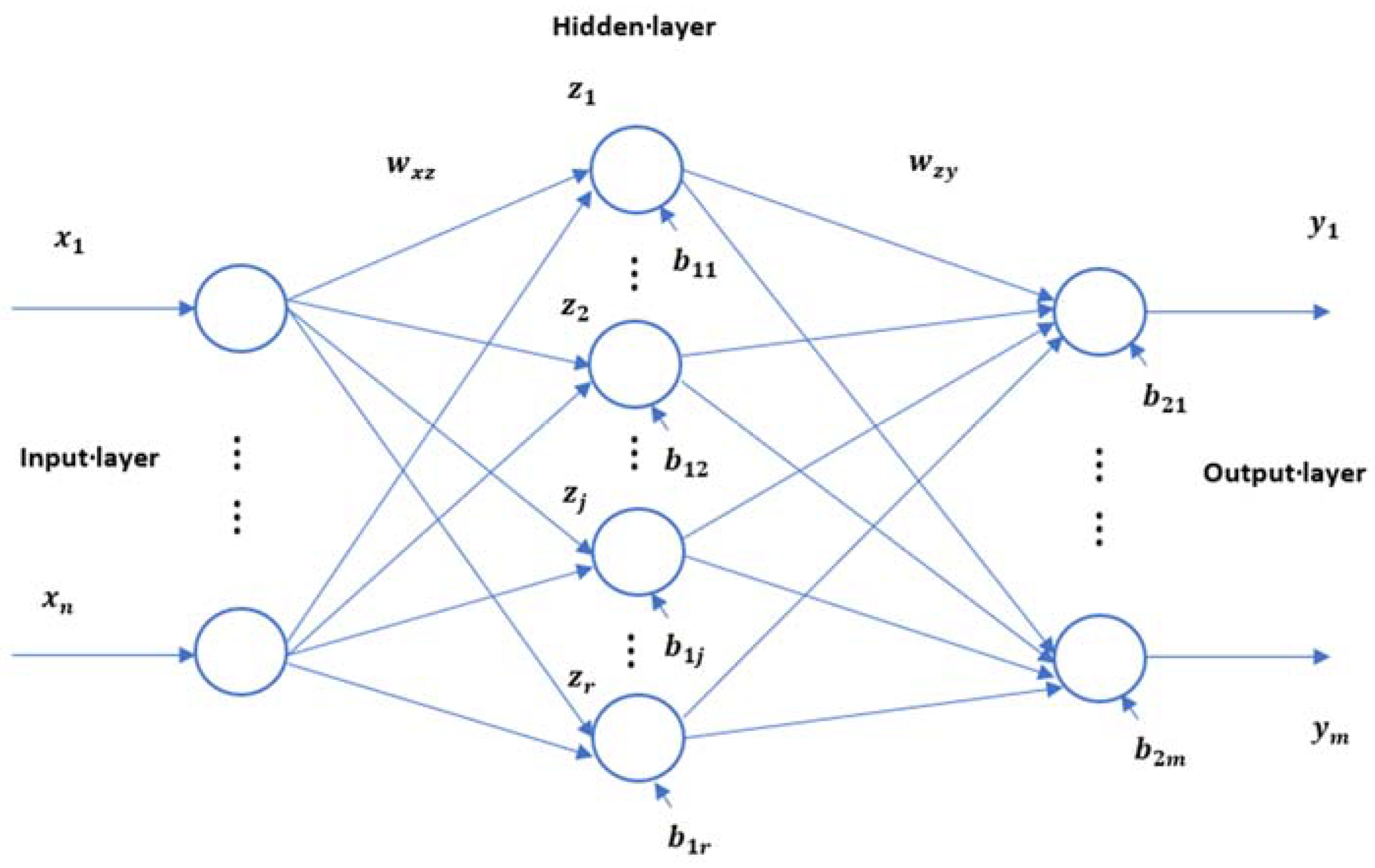
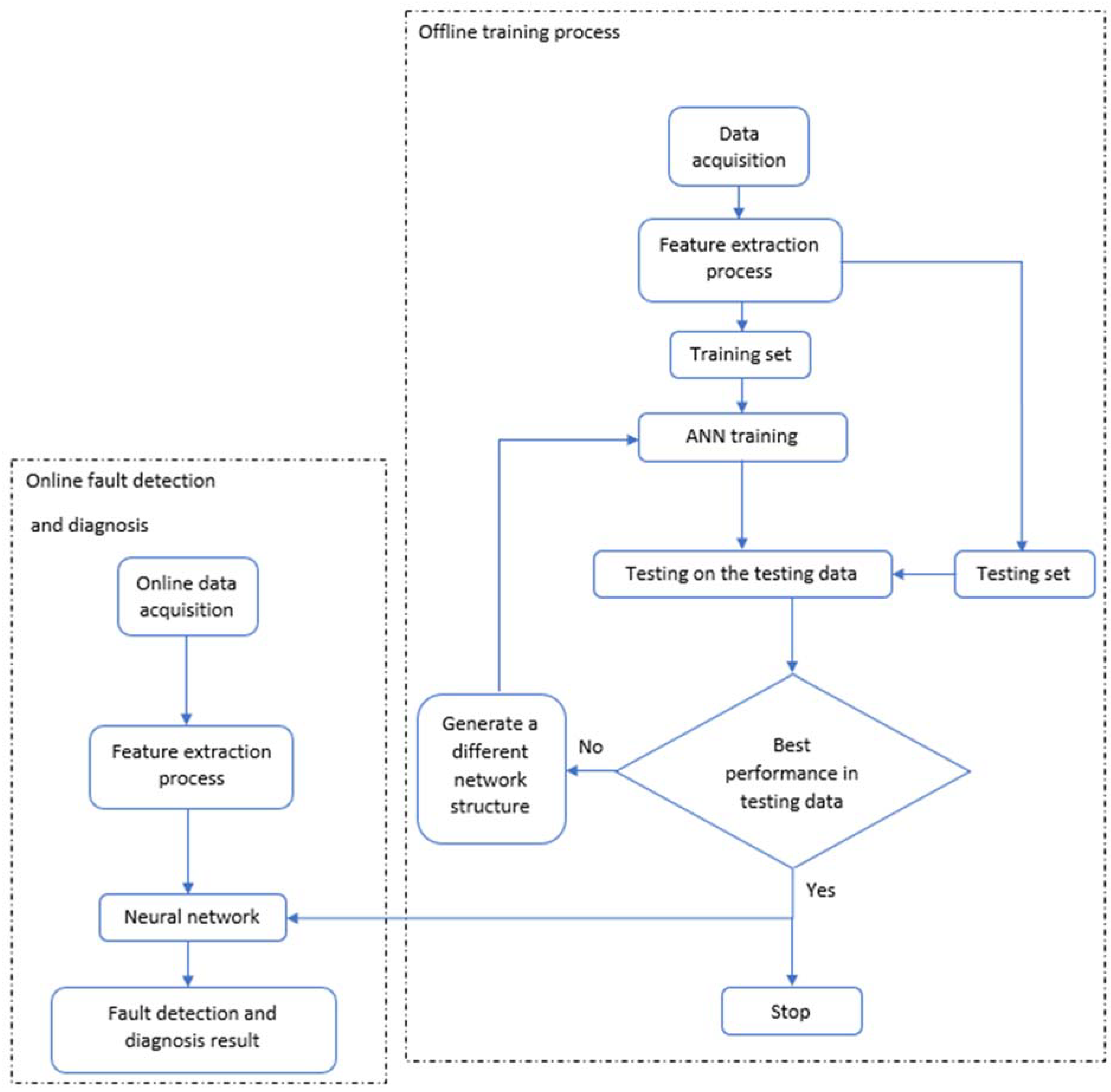
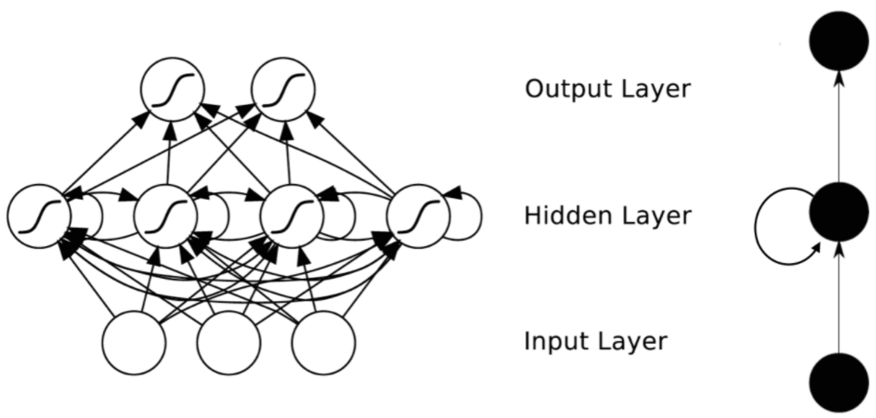
The Artificial Neural Networks Approach

ANN is a data processing model like the human nervous system, which includes neuron nodes and weights. The nodes are the basic processing units and are arranged into layers. Neurons in the input layer receive inputs from the outside world and neurons in the output layer give out the neural network processing results. The layers between the input and output layers are called hidden layers and the neurons in these layers are known as hidden neurons. The neurons in the adjacent layers are connected and the weights indicate the strength of the connections between the nodes. It abstracts the human nervous system from the perspective of data processing by building individual neuron models and forming various types of networks according to different connections and weights. ANNs mimic the human nervous system in that they can learn from example data by changing their structure and connection weights so that they can learn the relationship between the input and output variables. Common ANNs include back propagation (BP) neural networks, radial basis function (RBF) neural networks, self-organizing competitive (SC) neural networks, etc. This paper only introduces BP neural networks in detail as they are the most widely used.

A BP neural network is a multi-layer feed-forward neural network consisting of non-linear units with an input layer, implicit (hidden) layers, and an output layer, with full connectivity between the adjacent layers and no interconnection between units in the same layer. A typical 3-layer BP neural network structure is given in Figure 3. The BP algorithm is the fundamental approach for training ANNs, which is simply a problem of finding the minimum of the error function and allows for the weight modification of a multi-layer feed-forward neural network. The BP network training process contains two stages: the forward propagation of information and the backward propagation of error. Forward propagation means that the neurons in the input layer receive incoming stimuli and transfer them, after interacting with the weights and biases, to the neurons in the hidden layer, which in turn process the received information and then pass to the output layer neurons through the connection weights. The calculated network outputs are compared with the corresponding target values to work out the neural network prediction errors. The neural network prediction errors are then processed backwards layer by layer to retrieve the deviation of each layer’s weights and biases, which are subsequently modified. The whole procedure consists of alternating forward propagation of information and backward propagation of error until the output errors are sufficiently small.

Take the BP neural network layout with a single hidden layer as an example and suppose that $\mathrm{n}$ is the number of neurons in the input layer ($\mathrm{i}$ is the index number of neurons), $\mathrm{l}$ is the number of neurons in the hidden layer ($\mathrm{j}$ is the index number of neurons), and $\mathrm{m}$ is the number of neurons in the output layer ($\mathrm{k}$ is the index number of neurons). ${\mathrm{W}}_{\mathrm{ij}}$ represents the weight between the input layer and the hidden layer neurons, whereas ${\mathrm{W}}_{\mathrm{jk}}$ represents the weight between the hidden layer and the output layer neurons. ${\mathrm{b}}_{\mathrm{j}}$ represents the bias of neurons in the hidden layer, whereas ${\mathrm{b}}_{\mathrm{k}}$ represents the bias of neurons in the output layer. The forward propagation of information is represented as follow:

$${\mathrm{y}}_{\mathrm{j}}=\mathrm{f}\left({\displaystyle \sum }_{\mathrm{i}=1}^{\mathrm{n}}{\mathrm{W}}_{\mathrm{ij}}{\mathrm{x}}_{\mathrm{i}}{+\mathrm{b}}_{\mathrm{j}}\right)$$

(9)

$${\mathrm{z}}_{\mathrm{k}}=\mathrm{f}\left({\displaystyle \sum }_{\mathrm{j}=1}^{\mathrm{l}}{\mathrm{W}}_{\mathrm{jk}}{\mathrm{y}}_{\mathrm{j}}{+\mathrm{b}}_{\mathrm{k}}\right)$$

(10)

where ${\mathrm{x}=(\mathrm{x}}_1{,\mathrm{x}}_2,\cdots {,\mathrm{x}}_{\mathrm{n}})$ represents the input vector of the input layer, ${\mathrm{y}=(\mathrm{y}}_1{,\mathrm{y}}_2,\cdots {,\mathrm{y}}_{\mathrm{l}})$ represents the output vector of the hidden layer, and ${\mathrm{z}=(\mathrm{z}}_1{,\mathrm{z}}_2,\cdots {,\mathrm{z}}_{\mathrm{m}})$ represents the output vector of the output layer. Let ${\mathrm{z}}^{*}{=(\mathrm{z}}_1^{*}{, \mathrm{z}}_2^{*},\cdots {, \mathrm{z}}_{\mathrm{m}}^{*})$ be the desired output vector, $\mathrm{E}$ represents the error function which is typically half of the sum of squared errors, and $\mathsf{\eta }$ represents the learning rate in BP neural networks. The standard BP neural network modifies the weights and bias according to the negative gradient of the error function, and the backward propagation process of the errors is represented as follow:

$$\mathrm{E}=\frac{1}{2}{\displaystyle \sum }_{\mathrm{k}=1}^{\mathrm{m}}{\left({\mathrm{z}}_{\mathrm{k}}^{*}{-\mathrm{z}}_{\mathrm{k}}\right)}^2$$

(11)

$$\Delta {\mathrm{W}}_{\mathrm{jk}}=-\mathsf{\eta }\frac{\mathrm{\partial }\mathrm{E}}{\partial {\mathrm{W}}_{\mathrm{jk}}}=\mathsf{\eta }\left({\mathrm{z}}_{\mathrm{k}}^{*}{-\mathrm{z}}_{\mathrm{k}}\right){\mathrm{y}}_{\mathrm{j}}{\mathrm{f}}^{\prime }\left({\displaystyle \sum }_{\mathrm{j}=1}^{\mathrm{l}}{\mathrm{W}}_{\mathrm{jk}}{\mathrm{y}}_{\mathrm{j}}{-\mathrm{b}}_{\mathrm{k}}\right)$$

(12)

$$\Delta {\mathrm{b}}_{\mathrm{k}}=-\mathsf{\eta }\frac{\partial \mathrm{E}}{\partial {\mathrm{b}}_{\mathrm{k}}}=\mathsf{\eta }\left({\mathrm{z}}_{\mathrm{k}}{-\mathrm{z}}_{\mathrm{k}}^{*}\right){\mathrm{f}}^{\prime }\left({\displaystyle \sum }_{\mathrm{j}=1}^{\mathrm{l}}{\mathrm{W}}_{\mathrm{jk}}{\mathrm{y}}_{\mathrm{j}}{-\mathrm{b}}_{\mathrm{k}}\right)$$

(13)

$$\Delta {\mathrm{W}}_{\mathrm{ij}}=-\mathsf{\eta }\frac{\partial \mathrm{E}}{\partial {\mathrm{W}}_{\mathrm{ij}}}{=\mathsf{\eta }\mathrm{x}}_{\mathrm{i}}{\mathrm{f}}^{\prime }\left({\displaystyle \sum }_{\mathrm{i}=1}^{\mathrm{n}}{\mathrm{W}}_{\mathrm{ij}}{\mathrm{x}}_{\mathrm{i}}{-\mathrm{b}}_{\mathrm{j}}\right){\displaystyle \sum }_{\mathrm{k}=1}^{\mathrm{m}}{\mathrm{W}}_{\mathrm{jk}}{\mathrm{f}}^{\prime }\left({\displaystyle \sum }_{\mathrm{j}=1}^{\mathrm{l}}{\mathrm{W}}_{\mathrm{jk}}{\mathrm{y}}_{\mathrm{j}}{-\mathrm{b}}_{\mathrm{k}}\right)\left({\mathrm{z}}_{\mathrm{k}}^{*}{-\mathrm{z}}_{\mathrm{k}}\right)$$

(14)

$$\Delta {\mathrm{b}}_{\mathrm{j}}=-\mathsf{\eta }\frac{\partial \mathrm{E}}{\partial {\mathrm{b}}_{\mathrm{j}}}{=\mathsf{\eta }\mathrm{f}}^{\prime }\left({\displaystyle \sum }_{\mathrm{i}=1}^{\mathrm{n}}{\mathrm{W}}_{\mathrm{ij}}{\mathrm{x}}_{\mathrm{i}}{-\mathrm{b}}_{\mathrm{j}}\right){\displaystyle \sum }_{\mathrm{k}=1}^{\mathrm{m}}{\mathrm{W}}_{\mathrm{jk}}{\mathrm{f}}^{\prime }\left({\displaystyle \sum }_{\mathrm{j}=1}^{\mathrm{l}}{\mathrm{W}}_{\mathrm{jk}}{\mathrm{y}}_{\mathrm{j}}{-\mathrm{b}}_{\mathrm{k}}\right)\left({\mathrm{z}}_{\mathrm{k}}{-\mathrm{z}}_{\mathrm{k}}^{*}\right)$$

(15)

Once the adjustments for the weights and bias are found, the network weights and bias can be updated, and then the process of forward propagation of information, backward propagation of errors, and adjustments of weights and bias calculated again until the iteration termination condition is met.

Neural networks have received increasing interest from academics and have been used in the field of equipment condition monitoring as artificial intelligence algorithms have advanced. The condition information of a device is the carrier of condition diagnosis, and different types of condition information respond to different degrees of the device’s condition, so to achieve condition monitoring, scholars have tried to train ANN models with different condition information, which can be vibration, noise, temperature, pressure, acoustic emission, and so on [93,94,95,96,97,98,99,100,101,102]. Vibration signals are used more frequently. In [103], Patel et al. used the wavelet packet transform to extract statistical features from the original bearing vibration signal and developed a bearing damage index (BID) to select the dominant wavelet packet transform to further extract statistical features from the vibration signal features and used the extracted features as inputs to an ANN model. The results show that ANN is more effective in fault detection and prediction than features extracted from the original signal when data from higher BDI vibration signals are selected. Jami et al. [40] decomposed the vibration signal of a centrifugal pump impeller using time analysis (TA), frequency analysis (FA) and wavelet packet transform (WPT) respectively to obtain the time domain statistical parameters, frequency domain peaks and time frequency domain wavelet packet energy presented as feature datasets. ANN fault diagnosis models were established for each of these three data sets. After adjusting the network nodes and transfer functions, the results show that the feature datasets obtained after WPT analysis can better represent the fault information and have higher diagnostic performance for pump impellers under different operating conditions. In [41], a non-linear auto-regression (NLAR) model was developed based on the time series of pump casing vibration signals under non-fault conditions, with a multilayer neural network as the non-linear estimator. Compared to the Fast Fourier Transform (FFT) based diagnostic method, the ANN based NLAR model can effectively detect faults at the early stage and is successfully applied to pump cavitation fault detection. Sharma et al. [104] obtained the frequency domain characteristics of the vibration signals of three-phase asynchronous induction motor ball bearings under different conditions by frequency domain analysis. These features were used to train an ANN classifier model, which ultimately enabled fault diagnosis of defects in the inner and outer rings of the bearings. In addition to the use of vibration signals, current signals and temperature signals are often used as state information for the training of ANN models. In [89], Refaat et al. decomposed the stator current signal of a three-phase motor into an intrinsic mode function (IMF) containing the main amplitude and frequency information by means of the empirical mode decomposition (EMD) method. The IMFs were then applied to the Wigner-Ville distribution (WVD) to obtain WVD contour patterns to characterize the characteristic frequencies of bearing defects. The contour pattern is then pattern recognized using an ANN, which can effectively detect outer ring defects in bearings. Sheikh et al. [105] transformed the induction motor current signal into a two-dimensional park vector (PV) pattern image by the park vector analysis (PVA) method. The different features of the pattern image (Area of PV pattern; Circumference of the pattern; width of the pattern; resultant of the centroid) were then used as inputs to the ANN and the motor bearing state as output from the ANN, enabling the detection and diagnosis of faults caused by mis-mounted bearings. This enables the detection and diagnosis of defects caused by incorrectly mounted bearings. Bangalore and Tjernberg [106] constructed the detected average temperature signals of the wind turbine gearbox bearings into bearing behaviour patterns via the SCADA system. The alarm and warning feature data from the SCADA system were then used to train the ANN model. The results show that the method can efficiently and accurately detect failures due to spalled or damaged bearings. Additionally, in addition to employing a single signal as state information, multiple signals are often used in combination to train ANN-based state detection models. For instance, in [107], Verma et al. transformed the sample entropy (SampEn) into the multiscale entropy of the current and vibration signals of an induction motor into a time series and used it as input to an ANN for misalignment fault detection of induction motors. This approach not only reduces the number of sensors, but also avoids the need for extensive calculations in the frequency domain analysis. Sharma et al. [108] used the data set of electric submersible pump (ESP) system variables obtained from real-time sensor monitoring and the corresponding combination of variables calculated (e.g., temperature, pressure, etc.) as input to an ANN, with the input weights of the variables determined by the severity of their impact on the system. Afterwards, the inputs are compared with the operating ranges corresponding to the ESP components in the hidden layer, and finally the output layer determines whether the input conditions will lead to an ESP failure or predict the trend leading to an ESP failure. In [90], the current signal is analyzed by performing a third harmonic analysis to extract the amplitude and frequency features of the fault, and the vibration signal is decomposed into intrinsic mode functions (IMFs) using complete ensemble empirical mode decomposition (CEEMD) to extract the signal features with the best IMFs in the time and frequency domains. Afterwards, the features of the current and vibration signals that are most relevant to the health indicators are combined and reduced to two-dimensional primary metric space data using a PCA model. This dataset was used to train the ANN model and achieved a diagnostic accuracy of 99% on the test data obtained under stator fault of a brushless DC motor.

Figure 4 shows the basic processes for condition monitoring using the ANN model, and the methods described next in this paper have the similar process to this method. The relevant references for the ANN methods discussed in this section are summarized in

Table 10. Motor condition monitoring using artificial neural networks.

References	Application	Type of Equipment	Signal	Fault Type
[89]	Fault detection and diagnosis	Induction motor	Current signal	Bearing fault (inner and outer race)
[90]	Fault diagnosis	Permanent magnet Brushless DC motor	Current and vibration signal	Stator and rotor faults
[93]	Fault diagnosis	Induction motor	Current and vibration signal	Various types of motor faults such as bearing, stator, rotor, and eccentricity
[94]	Condition diagnosing and remaining useful life predicting	Induction motor	Current and voltage signal	Turn-to-turn short circuit in one phase, turn-to-turn short circuit in two phases, missing phase, and two phases
[95]	Fault detection	Induction motor	Vibration signal	Unbalance
[101]	Fault detection	Induction motor	Current signal	Stator inter turn short circuit fault and unbalance supply voltage fault
[105]	Fault diagnosis	Induction motor	Current signal	Defective due to misalignment of bearing installation (misalignment, shaft deflect, outer race damage, and inner race damage)
[107]	Fault detection	Induction motor	Current and vibration signal	Misalignment faults

,

Table 11. Pump condition monitoring using artificial neural networks.

References	Application	Type of Equipment	Signal	Fault Type
[39]	Fault detection	Centrifugal pump	Vibration signals	Cavitation Vans tip fault Impeller crack fault
[40]	Fault detection	Centrifugal pump	Impeller vibration signal	Cracks and imbalances in impellers of varying degrees are simulated manually by making port dramas and hammer blows. (Impeller damage due to corrosion in the fluid and external solids materials)
[41]	Fault detection	Gear pump	Pump casing vibration signal	Abrupt changes in the behavior caused by cavitation
[68]	Fault diagnosis	Airborne fuel pump	Vibration and pressure signal	Blade damage, diffusion tube damage, leakage, diffusion tube impeller rub, bearing wear
[96]	Malfunction detection	Shimizu PS-128BT water pump	Vibration signal (bearing, impeller, and capacitor)	Broken capacitor, broken impeller, broken bearing, broken capacitor & impeller, and broken capacitor & bearing
[100]	Fault diagnosis	Reactor coolant pump	Vibration signal	Bearing wear; rotor mass eccentricity; impeller mass eccentricity; wear ring abrasion
[102]	Fault detection	Circulating water pump	Bearing temperature signal	Broken bearings, damaged bearings, high cooling water temperatures, noisy equipment, etc.
[108]	Predict failure	Real-time data collected over a period of operation of electric submersible pumps (containing the information from surface and downhole data)	Pump discharge temperature, pump intake pressure, pump discharge pressure and so on.	Higher Flow rates, low pump intake pressures. Gas production, gas to oil ratio, leading to decrease in pump throughput. High Fluid Viscosity leading to pump failures. Pump being used outside its operating range. Corrosion and depositions leading to blockages in pump, debris in pump, shaft failures due to broken shafts, change in downhole pressure, blockage at perforations and pump intake.

and

Table 12. Bearing condition monitoring using artificial neural networks.

References	Application	Type of Equipment	Signal	Fault Type
[47]	Fault diagnosis	Rolling bearings	Vibration signal	Inner race and outer race faults
[78]	Fault diagnosis	Locomotive roller bearing	Vibration signal	Slight rub fault in the outer race, Serious flaking fault in the outer race, Slight rub fault in the inner race, Roller rubs fault, Compound faults in the outer and inner races, compound faults in the outer race and rollers, compound faults in the inner race and rollers, compound faults in the outer and inner races and rollers
[97]	Remaining useful life prediction	Rolling bearing	Vibration signals	Inner race, ball, and outer race fault
[98]	Fault diagnosis	Rolling bearing	Vibration signal	Local spalls fault and Pits or distributed surface wear fault
[99]	Fault prognosis	Rolling bearing	Vibration signal	Inner race, ball, and outer race fault
[103]	Fault detection and prognosis	Rolling bearing	Bearing vibration signal	Inner race, ball, and outer race fault
[104]	Fault diagnosis	Rolling bearing	Bearing vibration signal	Inner race and outer race faults
[106]	Fault detection	Rolling bearing	Temperature measurement for five bearings	Damaged due to spalling in the bearing.

.

The Support Vector Machine (SVM) Approach

The initial objective of SVM theory was to devise a method for dealing with classification issues by locating an optimum classification hyperplane that meets the classification requirements, and by maximizing the blank area on both sides of the hyperplane. Theoretically, SVM is capable of obtaining optimum classification for two-dimensional linearly divisible data.

Consider the classification of two data types as an example, given a training sample set ${\mathrm{D}}_{\mathrm{i}}=\left({\mathrm{x}}_{\mathrm{i}}{,\mathrm{y}}_{\mathrm{i}}\right), \mathrm{i}=1,2,\cdots ,\mathrm{l}, \mathrm{x}\in {\mathrm{R}}^{\mathrm{n}}, \mathrm{y}\in \left\{\pm 1\right\}$, where $\mathrm{x}$ is the input sample, $\mathrm{y}$ is the category value, and $\left(\mathsf{\omega }·\mathrm{x}\right)+\mathrm{b}=0 (\mathsf{\omega }\in {\mathrm{R}}^{\mathrm{n}}, \mathrm{b}\in \mathrm{R})$ is the hyperplane, in order for the classification plane to accurately classify all samples and have a classification interval, it is important to verify that the hyperplane meets the constraint ${\mathrm{y}}_{\mathrm{i}}\left[{(\mathsf{\omega }\mathrm{x}}_{\mathrm{i}}+\mathrm{b})\right]\ge 1, \mathrm{i}=1,2,\cdots \mathrm{l}$. Therefore, the task of generating the optimal hyperplane becomes the problem of obtaining the minimal value within the restrictions.

$$\min \frac{1}{2}{\Vert \mathsf{\omega }\Vert }^2$$

(16)

The Lagrange function is introduced to resolve this restricted optimization issue.

$$\left(\mathsf{\omega },\mathrm{b},\mathsf{\alpha }\right)=\frac{1}{2}{\Vert \mathsf{\omega }\Vert }^2-{\displaystyle \sum }_{\mathrm{i}=1}^{\mathrm{l}}{\mathsf{\alpha }}_{\mathrm{i}}\left({\mathrm{y}}_{\mathrm{i}}\left({\mathsf{\omega }\mathrm{x}}_{\mathrm{i}}+\mathrm{b}\right)-1\right)$$

(17)

where, ${\mathsf{\alpha }}_{\mathrm{i}} > 0$ is the Lagrange multiplier for each sample. Letting the partial derivatives of Equation (18) be zero for $\mathrm{b}$ and $\mathsf{\omega }$ respectively, it can be derived that:

$$\mathsf{\omega }={\displaystyle \sum }_{\mathrm{i}=1}^{\mathrm{l}}{\mathsf{\alpha }}_{\mathrm{i}}{\mathrm{y}}_{\mathrm{i}}{\mathrm{x}}_{\mathrm{i}}$$

(18)

$${\displaystyle \sum }_{\mathrm{i}=1}^{\mathrm{l}}{\mathsf{\alpha }}_{\mathrm{i}}{\mathrm{y}}_{\mathrm{i}}=0$$

(19)

The solution vector’s expansion consists of a subset of training sample vectors, none of which have zero Lagrange multipliers, i.e., the support vector. A sample vector with zero Lagrange multipliers contributes zero and is irrelevant for selecting a classification hyperplane. Therefore, a decision function describing the optimal classification hyperplane, also known as a support vector machine, is obtained from the training set, and its classification function is determined by the support vector.

$$\mathrm{f}\left(\mathrm{x}\right)=\mathrm{sgn}\left({\displaystyle \sum }_{\mathrm{i}=1}^{\mathrm{m}}{\mathsf{\alpha }}_{\mathrm{i}}{\mathrm{y}}_{\mathrm{i}}\left(\mathrm{x}·{\mathrm{x}}_{\mathrm{i}}\right)+\mathrm{b}\right)$$

(20)

In the field of condition monitoring SVM is mainly used for classification problems [109,110,111,112,113,114,115,116,117]. Compared to ANN, SVM is more suitable for small sample classification and is more efficient and accurate. In [118], when the current and vibration signals of the induction motor have been gathered, statistical characteristics are derived from their respective time domain data. Afterwards, the most effective features and the optimal SVM model parameters for fault diagnosis were chosen using a wraparound model and a grid search technique. Through fault diagnosis and prediction for diverse operating conditions of induction motors at different speeds and loads, a high level of precision can be achieved. The performance of diagnosis at an intermediate speed and load (which reflect the scenario of limited data) is also encouraging. Panda et al. [119] classified statistical characteristics taken from a centrifugal pump’s time-domain vibration data using SVM. Experiments were undertaken to identify two kinds of faults: flow obstructions and pump cavitation, each with a different fault severity and conditions. The results indicate that the SVM model gives more accuracy in predicting the beginning of cavitation events than the multi-class fault classification for different degrees of blockages. In [120], the time and frequency domain features of the bearing vibration signal are used to train an SVM model. The trained classifier can be used for real-time detection of inner race, outer race and rolling element faults in bearings. The Root mean square of vibration signal (RMS) features in the time domain are used for fault detection, while the energy content and energy deviation features in the frequency domain are used for fault classification. The experimental results show an accuracy of 86% and 96% for the detection of inner and outer race faults respectively. There are also modifications of the SVM, and optimized algorithms applied to the condition detection of equipment. For instance, in [60], Ebrahimi et al. used a fuzzy support vector machine (FSVM) to increase sensitivity to data and model generalization for the assessment of static and dynamic eccentricity fault severity in permanent magnet synchronous motors. The wavelet transform analysis of stator current features was used as training and testing data for the FSVM classifier, and it was determined that the model could accurately identify the type and degree of eccentricity and had a classification accuracy of 100% even in the presence of high noise. Since SVM can only perform binary classification, Gangsar et al. [121] have employed multiclass support vector machines (MSVM) to effectively diagnose and predict a broad variety of mechanical and electrical faults in induction motors. The time domain statistical features extracted from the current and vibration signals of the induction motor were then used to train the MSVM classifier. Several experiments demonstrate that the model can accurately predict all mechanical and electrical problems under varying loads. Some researchers also optimize the SVM parameters to achieve improved classification results. In [61], the frequency domain and wavelet analysis features of the vibration signals were extracted from various fault conditions of the pump under various operating conditions. These features serve as inputs to the SVM classifier to classify pump pipe blockage and cavitation faults. In addition, three optimization algorithms were used to determine the SVM classifier’s parameters for fault classification accuracy at higher pump speeds. The relevant references for the SVM methods discussed in this section are summarized in

Table 13. Motor condition monitoring using support vector machine.

References	Application	Type of Equipment	Signal	Fault Type
[60]	Fault diagnosis	Permanent magnet synchronous motor	Current, voltage signal and speed signal	Static and dynamic eccentricity fault
[109]	Fault diagnosis	Induction motor	Current and voltage signal	Inter-turn short-circuits, rotor, and bearing faults
[118]	Fault diagnosis	Induction motor	Current and vibration signal	Stator winding faults
[121]	Fault prognosis	Induction motor	Vibration and current signal	Bearing fault, unbalanced rotor fault, bowed rotor fault, rotor misalignment fault, broken-rotor bar fault, phase unbalance and single phasing fault with high resistance, phase unbalance and single phasing fault with low resistance, stator winding fault with high resistance and stator winding fault with low resistance

,

Table 14. Pump condition monitoring using support vector machine.

References	Application	Type of Equipment	Signal	Fault Type
[35]	Fault diagnosis	Plunger pump	Vibration signal	Swash plate wear and rotor wear
[57]	Fault diagnosis	Centrifugal pump	Vibration signal	Five mechanical faults (bearing, misalignment, unbalance, impeller, and looseness), and a hydraulic fault (cavitation)
[61]	Fault diagnosis	Centrifugal pump	Vibration signal	Suction flow blockages cavitations
[84]	Fault diagnosis	Aviation piston pump	Discharge pressure signal	loose piston defect
[110]	Fault diagnosis	Oil rig motor pump	Vibration signal	Misalignment, structural looseness, unbalance, hydrodynamic, mechanical looseness, rolling bearing
[111]	Fault diagnosis	Centrifugal pump	Vibration signal	Cavitation and impeller unbalance, cavitation and shaft misalignment, impeller unbalance and shaft misalignment
[112]	Fault diagnosis	Centrifugal pump	Vibration signal	Mechanical seal and Impeller faults
[115]	Condition evaluation	Canned motor pump	Performance parameters and the structure parameters of pump (flow, power consumption, stator temperature, winding insulation)	Severe or moderate degradation and normal or good condition
[116]	Condition prediction	Reactor coolant pump	Measurement variables	Variables out of control after a fault occurred
[117]	Fault diagnosis	Feed water pump	Vibration signal	Initial imbalance, rotor misalignment, rotor axial rubbing, thrust bearing damage, bearing looseness, bearing stiffness vary, foundation resonance, coupling damage
[119]	Fault prognosis	Centrifugal pump	Vibration signal	Flow blockages and cavitation

and

Table 15. Bearing condition monitoring using support vector machine.

References	Application	Type of Equipment	Signal	Fault Type
[46]	Fault detection	Rolling bearing	Vibration signal	Bearing faults
[73]	Fault detection and diagnosis	Bearing in main coolant pump and feed water pump	Vibration signal	Inner race; outer race and ball faults
[79]	Fault diagnosis	Rolling bearing	Vibration signal	Outer race, inner race, and ball faults
[83]	Fault diagnosis and prognosis	Rolling bearing	Vibration signal	Outer race, inner race, and ball faults
[113]	Fault diagnosis	Bearing form induction motor	Vibration signal	Ball, Inner race, and Outer race faults
[114]	Fault diagnosis	Rolling bearing	Vibration signal	Ball, Inner race, and Outer race faults
[120]	Early fault detection	A run-to-failure test conducted by Intelligent Maintenance Systems, University of Cincinnati, USA	Vibration signal	Roller, Inner race, and Outer race faults

.

The Extreme Learning Machine Approach

In traditional neural network training algorithms, many iterations of training are involved. This parameter adjustment process is not only time-consuming, but also computationally intensive, resulting in low network training efficiency. In the implementation of the algorithm, it is easy to generate local minima and has poor applicability. To address the above problems, Huang et al. [13]. proposed the ELM neural network. In contrast to previous single-hidden-layer feedforward neural networks, the ELM randomly selects weights and biases in the hidden layer, and then calculates the weights in the output layer by a regularized linear regression method.

The number of neurons in the input, hidden and output layers are $\mathrm{n}, \mathrm{l}, \mathrm{m}$, respectively. Let the connection weights between the input layer to the hidden layer and the hidden layer to the output layer be w and v respectively:

$$\mathrm{w}=\left[\begin{array}{c}{\mathrm{w}}_1\\ {\mathrm{w}}_2\\ \cdots \\ {\mathrm{w}}_{\mathrm{l}}\end{array}\right]={\left[\begin{array}{cccc}{\mathrm{w}}_{11}& {\mathrm{w}}_{12}& \cdots & {\mathrm{w}}_{1\mathrm{n}}\\ {\mathrm{w}}_{21}& {\mathrm{w}}_{22}& \cdots & {\mathrm{w}}_{2\mathrm{n}}\\ \cdots & \cdots & \ddots & ⋮\\ {\mathrm{w}}_{\mathrm{l}1}& {\mathrm{w}}_{\mathrm{l}2}& \cdots & {\mathrm{w}}_{\ln }\end{array}\right]}_{\mathrm{l}\times \mathrm{n}}$$

(21)

$$\mathrm{v}=\left[\begin{array}{c}{\mathrm{v}}_1\\ {\mathrm{v}}_2\\ \cdots \\ {\mathrm{v}}_{\mathrm{l}}\end{array}\right]= {\left[\begin{array}{cccc}\mathrm{v}& {\mathrm{v}}_{12}& \cdots & {\mathrm{v}}_{1\mathrm{n}}\\ {\mathrm{v}}_{21}& {\mathrm{v}}_{22}& \cdots & {\mathrm{v}}_{2\mathrm{n}}\\ \cdots & \cdots & \ddots & ⋮\\ {\mathrm{v}}_{\mathrm{l}1}& {\mathrm{v}}_{\mathrm{l}2}& \cdots & {\mathrm{v}}_{\mathrm{lm}}\end{array}\right]}_{\mathrm{l}\times \mathrm{m}}$$

(22)

The hidden layer bias is given as:

$$\mathrm{b}=\left[\begin{array}{c}{\mathrm{b}}_1\\ {\mathrm{b}}_2\\ \cdots \\ {\mathrm{b}}_{\mathrm{l}}\end{array}\right]$$

(23)

The activation function is $\mathrm{g}\left(\mathrm{x}\right)$, then for an output $\mathrm{Y}$ with $\mathrm{N}$ samples can be expressed as:

$$\mathrm{Y}=\mathrm{Hv}$$

(24)

where, $\mathrm{H}$ is the hidden layer output matrix:

$$\mathrm{H}={\left[\begin{array}{cccc}\mathrm{g}\left({\mathrm{w}}_1·{\mathrm{x}}_1{+\mathrm{b}}_1\right)& \mathrm{g}\left({\mathrm{w}}_2·{\mathrm{x}}_2{+\mathrm{b}}_2\right)& \cdots & \mathrm{g}\left({\mathrm{w}}_{\mathrm{l}}·{\mathrm{x}}_1{+\mathrm{b}}_{\mathrm{l}}\right)\\ \mathrm{g}\left({\mathrm{w}}_1·{\mathrm{x}}_2{+\mathrm{b}}_1\right)& \mathrm{g}\left({\mathrm{w}}_2·{\mathrm{x}}_2{+\mathrm{b}}_2\right)& \cdots & \mathrm{g}\left({\mathrm{w}}_1·{\mathrm{x}}_2{+\mathrm{b}}_{\mathrm{l}}\right)\\ \cdots & \cdots & \ddots & ⋮\\ \mathrm{g}\left({\mathrm{w}}_1·{\mathrm{x}}_{\mathrm{N}}{+\mathrm{b}}_1\right)& \mathrm{g}\left({\mathrm{w}}_2·{\mathrm{x}}_{\mathrm{N}}{+\mathrm{b}}_2\right)& \cdots & \mathrm{g}\left({\mathrm{w}}_1·{\mathrm{x}}_{\mathrm{N}}{+\mathrm{b}}_{\mathrm{l}}\right)\end{array}\right]}_{\mathrm{N}\times \mathrm{l}}$$

(25)

The following theorem was proposed by Huang et al.:

Given a single hidden layer forward neural network (SLFN) with $\mathrm{N}$ hidden layer neurons, $\mathrm{N}$ distinct samples ${(\mathrm{x}}_{\mathrm{i}}{, \mathrm{y}}_{\mathrm{i}})$, where ${\mathrm{x}}_{\mathrm{i}}{=[\mathrm{x}}_{\mathrm{i}1}{, \mathrm{x}}_{\mathrm{i}2}, \cdots {,\mathrm{x}}_{\mathrm{in}}{]}^{\mathrm{T}}\in {\mathrm{R}}^{\mathrm{n}}$ and ${\mathrm{y}}_{\mathrm{i}}{=[\mathrm{y}}_{\mathrm{i}1}{, \mathrm{y}}_{\mathrm{i}2}, \cdots {,\mathrm{y}}_{\mathrm{im}}{]}^{\mathrm{T}}\in {\mathrm{R}}^{\mathrm{m}}$, and an infinitely differentiable function $\mathrm{g}\left(\mathrm{x}\right)$, then for any assignment ${\mathrm{w}}_{\mathrm{i}}\in {\mathrm{R}}^{\mathrm{n}}$ and ${\mathrm{b}}_{\mathrm{i}}\in \mathrm{R}$, there is a hidden layer output matrix $\mathrm{H}$ that is invertible and satisfies $\Vert \mathrm{Hv}-\mathrm{Y}\Vert =0$.

Given $\mathrm{N}$ distinct samples ${(\mathrm{x}}_{\mathrm{i}}{, \mathrm{y}}_{\mathrm{i}})$, where ${\mathrm{x}}_{\mathrm{i}}{=[\mathrm{x}}_{\mathrm{i}1}{, \mathrm{x}}_{\mathrm{i}2}, \cdots {,\mathrm{x}}_{\mathrm{in}}{]}^{\mathrm{T}}\in {\mathrm{R}}^{\mathrm{n}}$ and ${\mathrm{y}}_{\mathrm{i}}{=[\mathrm{y}}_{\mathrm{i}1}{, \mathrm{y}}_{\mathrm{i}2}, \cdots {,\mathrm{y}}_{\mathrm{im}}{]}^{\mathrm{T}}\in {\mathrm{R}}^{\mathrm{m}}$, and an infinitely differentiable function $\mathrm{g}\left(\mathrm{x}\right)$. Given any small error $\mathsf{\epsilon }(\mathsf{\epsilon } > 0)$, there exists a SLFN with $\mathrm{M} (\mathrm{M} \le \mathrm{N})$ hidden layer neurons that has a hidden layer output matrix $\mathrm{H}$ that is invertible and satisfies $\Vert \mathrm{Hv}-\mathrm{Y} \Vert < \mathsf{\epsilon }$ for any assignment ${\mathrm{w}}_{\mathrm{i}}\in {\mathrm{R}}^{\mathrm{n}}$ and ${\mathrm{b}}_{\mathrm{i}}\in \mathrm{R}$.

From the above two theorems, if the number of hidden layer neurons $\mathrm{l}$ and the number of training samples $\mathrm{N}$ are equal, then the network can approximate the samples with zero error for any $\mathrm{w}, \mathrm{b}$. Thus, training for the SLFN model is also equivalent to solving the Equation (25) for the least-and-multiply solution $\hat{\mathrm{v}}$.

$$\Vert \mathrm{H}({\hat{\mathrm{w}}}_1,\cdots ,{\hat{\mathrm{w}}}_{\mathrm{M}},{\hat{\mathrm{b}}}_1,\cdots ,{\hat{\mathrm{b}}}_{\mathrm{M}})\hat{\mathrm{v}}-\mathrm{Y}\Vert =\underset{\mathrm{v}}{min}\Vert \mathrm{H}({\mathrm{w}}_1,\cdots ,{\mathrm{w}}_{\mathrm{M}},{\mathrm{b}}_1,\cdots ,{\mathrm{b}}_{\mathrm{M}})\mathrm{v}-\mathrm{Y}\Vert$$

(26)

However, when $\mathrm{N}$ is large, an excessive number of hidden layers implies a larger computational effort, so the size of the hidden layers can be reduced to $\mathrm{M}$ so that the training error can be approximated by an arbitrarily small $\mathsf{\epsilon }$. In this case, the Moore-Penrose generalized inverse matrix ${\mathrm{H}}^{+}$ of $\mathrm{H}$ can be used to solve for Equation (26).

$$\hat{\mathrm{v}}={\mathrm{H}}^{+}\mathrm{Y}$$

(27)

The most common method currently used to solve the generalized inverse matrix ${\mathrm{H}}^{+}$ is the singular value decomposition method, regardless of whether ${\mathrm{H}}^{\mathrm{T}}\mathrm{H}$ is a singular or non-singular matrix, which is solved by the following equation.

$$\hat{\mathrm{v}}={\left({\mathrm{H}}^{\mathrm{T}}\mathrm{H}\right)}^{-1}{\mathrm{H}}^{\mathrm{T}}\mathrm{Y}$$

(28)

In contrast to traditional single hidden layer feedforward neural networks, ELM randomly selects weights and biases in the hidden layer and then calculates the weights of the output layer by a regularized linear regression method. Even though the weights of the hidden layer are randomly generated, ELM maintains the universal approximation capability of SLFN. Therefore, from the perspective of learning efficiency, ELM networks are not only simple to operate, but also learn faster and have better global search capability, which can overcome the problem of traditional neural networks falling into local optima, without generating overfitting or inappropriate learning rates, and have better generalization capability.

Compared to standard ANN and SVM algorithms, the rapid training speed and excellent learning efficiency of ELM have brought it into focus for equipment condition monitoring [62,91,122,123,124,125]. In [126], the RMS values of the voltage and current characteristics of the three-phase induction motor are used as ELM model inputs. Six external faults of the three-phase induction motor were discovered, with ELM providing faster results and reducing the computational load more effectively than SVM and MLP. In [42], the Fourier spectrum features of eight manually collected motor pump vibration signals are utilized as input to an ELM model to categorize motor pump faults such as misalignment, unbalance, and rubbing. When compared to other statistical classifiers (K-Nearest-Neighbor, SVM, etc.), the generalization and classification accuracy of the ELM were shown to be better to those of the statistical classifiers. In [127], Lan et al. extracted information from the vibration signal of a faulty hydraulic pump using three different signal processing techniques. The retrieved signal features that are most sensitive to the fault are utilized to train the classifier model. Comparing ELM, BP, and SVM classifiers revealed that ELM has benefits in terms of training speed and generalization and is easier in terms of model construction and parameter selection than the other two approaches. In the sphere of condition monitoring, the combination of ELM and signal pre-processing techniques has also garnered considerable interest. By integrating ELM with a depth wavelet autoencoder in [128], ELM was able to classify bearing faults with better accuracy. Multiple wavelet auto-encoders were utilized to create a depth wavelet autoencoder that efficiently captures the vibration signal’s features. The recorded features are then fed into an ELM model to identify various bearing faults. The experimental results demonstrated that the suggested technique achieves over 95% accuracy, which is much greater than classic ELM, wavelet neural network, BP neural network, and SVM.

The relevant references for the ELM methods discussed in this section are summarized in

Table 16. Equipment condition monitoring using extreme learning machine.

Equipment	References	Application	Type of Equipment	Signal	Fault Type
Motor	[126]	Fault classification	Induction motor	Voltage and current signal	External faults (Mechanical, environmental, and electrical faults)
Pump	[62]	Fault diagnosis	Hydraulic pump	Vibration signal	Slipper loosing and Valve plate wear fault
	[122]	Fault diagnosis	Hydraulic pump	Sound signal	Single slipper wear, single slipper loose, swash plate wear, and combined faults
	[91]	Fault diagnosis	Hydraulic pump	Vibration signal	Single slipper wear, single slipper loose, and center spring wear faults
	[42]	Fault classification	Motor pump	Vibration signal	Misalignment unbalance rubbing accelerometer fault
	[127]	Fault detection	Hydraulic pump	Vibration signal	Slipper abrasion
Bearing	[123]	Fault diagnosis	Rolling bearing	Vibration signal	Ball, inner race, and outer race faults
	[124]	Fault diagnosis	Rolling bearing	Vibration signal	Ball, inner race, and outer race faults
	[125]	Fault diagnosis	Rolling bearing	Vibration signal	Ball, inner race, and outer race faults
	[128]	Fault diagnosis	Rolling bearing	Vibration signal	Ball, inner race, and outer race faults

.

2.2.2. Method Based on Deep Learning

As an extension and evolution of machine learning, deep learning is based on neural networks but is distinct from them. It solves the inherent problems of traditional neural networks by learning the data representation layer by layer through a multi-hidden layer network structure. It has been widely implemented in the fields of image processing and text recognition, but industrial equipment condition monitoring is still in the research phase. Deep belief networks (DBN), convolutional neural networks (CNN), and recurrent neural networks (RNN) are the most common deep learning models at present.

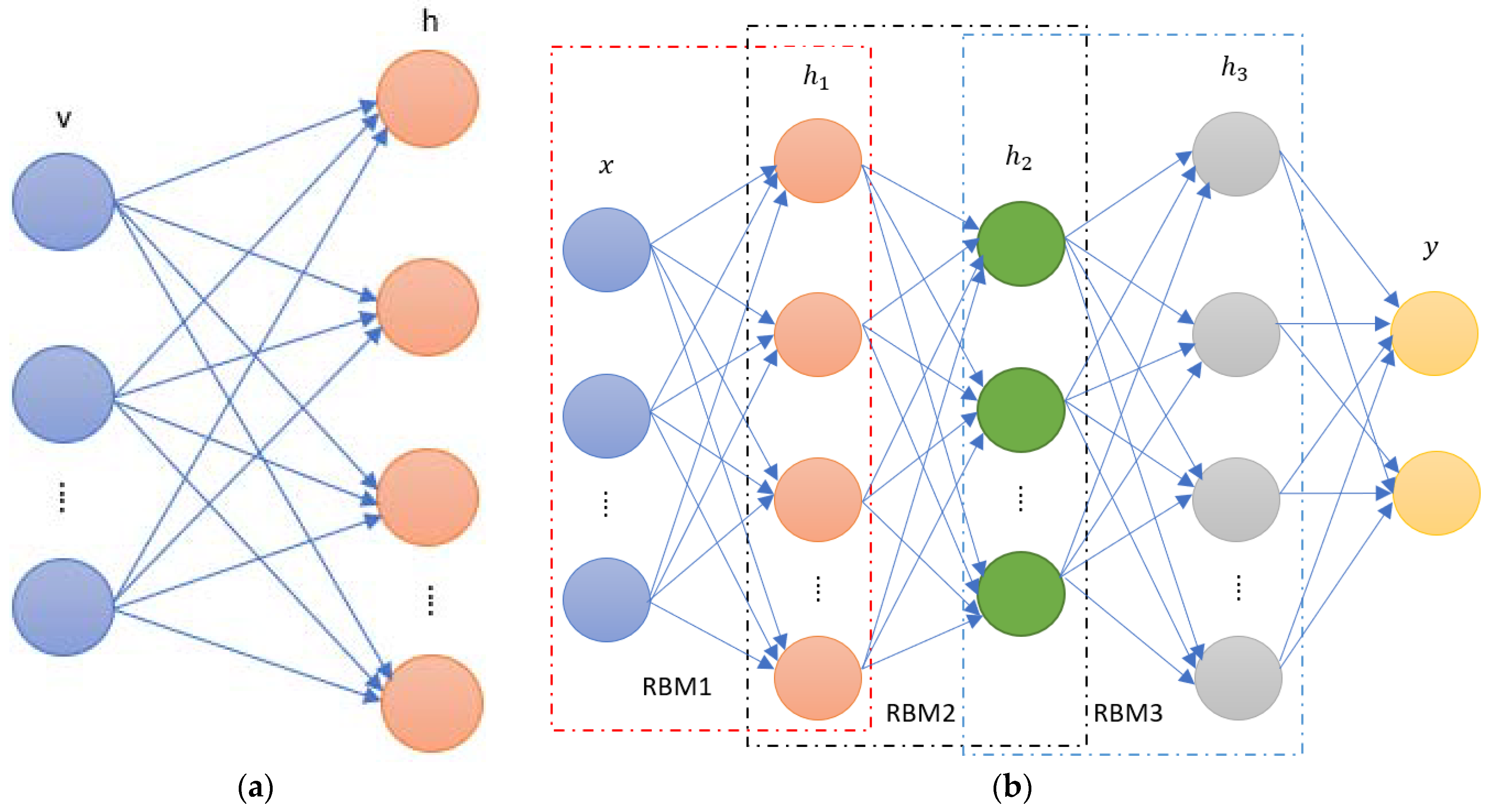
The Deep Belief Network Approach

As shown in Figure 5, a DBN is multi-hidden layer probabilistic generative model consisting of multiple restricted Boltzmann machines (RBM) and one output layer (usually a classification layer) combined to build a joint distribution between observed data and labels by training layer by layer. Unlike the directed/unidirectional connectivity of the hidden layers in DBNs, RBMs are multi-hidden Boltzmann networks in which the hidden layers both convey information and allow for top-down feedback adjustment.

The RBM can derive potential feature representations from the training data distribution. It is assumed that the activation conditions of each hidden unit are independent for a given input data again, and conversely, the activation conditions of the visible units are independent for a given hidden unit state. The model structure of the RBM consists of the weight matrix $\mathrm{W}$ of size $\mathrm{m} \times \mathrm{n}$, each element ${\mathrm{w}}_{\mathrm{ij}}$ in this matrix is associated with the corresponding visible layer neuron state vector ${\mathrm{v}}_{\mathrm{i}}$ and hidden layer neuron state vector ${\mathrm{h}}_{\mathrm{j}}$. Also, each layer has a corresponding offset coefficient ${\mathrm{a}}_{\mathrm{i}}$ (for visible units) and ${\mathrm{b}}_{\mathrm{j}}$ (for hidden units). When given the model parameters $\mathsf{\theta }=[\mathsf{\omega }, \mathrm{a}, \mathrm{b}]$, the energy function of the RBM can be written as:

$$\mathrm{E}\left(\mathrm{v}, \mathrm{h}; \mathsf{\theta }\right)=-{\displaystyle \sum }_{\mathrm{i}}^{\mathrm{m}}{\displaystyle \sum }_{\mathrm{j}}^{\mathrm{n}}{\mathrm{w}}_{\mathrm{ij}}{\mathrm{v}}_{\mathrm{i}}{\mathrm{h}}_{\mathrm{j}}-{\displaystyle \sum }_{\mathrm{i}=1}^{\mathrm{m}}{\mathrm{a}}_{\mathrm{i}}{\mathrm{v}}_{\mathrm{i}}-{\displaystyle \sum }_{\mathrm{j}=1}^{\mathrm{n}}{\mathrm{b}}_{\mathrm{j}}{\mathrm{h}}_{\mathrm{j}}$$

(29)

where $\mathrm{m}$ and $\mathrm{n}$ represent the number of visible units and hidden units respectively.

The joint distribution of all units can be obtained from the calculation of the energy function $\mathrm{E}$:

$$\mathrm{p}\left(\mathrm{v},\mathrm{h};\mathsf{\theta }\right)=\frac{\exp \left(-\mathrm{E}\left(\mathrm{v},\mathrm{h};\mathsf{\theta }\right)\right)}{\mathrm{Z}}$$

(30)

where, $\mathrm{Z}={{\displaystyle \sum }}_{\mathrm{h},\mathrm{v}}\exp (-\mathrm{E}(\mathrm{v},\mathrm{h};\mathsf{\theta }\left)\right)$ is the normalization factor.

From the above it follows that the conditional probability of a hidden layer neuron being activated is:

$$\mathrm{p}\left({\mathrm{h}}_{\mathrm{j}}|\mathrm{v};\mathsf{\theta }\right)=\mathsf{\delta }\left({\mathrm{b}}_{\mathrm{j}}+{\displaystyle \sum }_{\mathrm{i}=1}^{\mathrm{m}}{\mathrm{w}}_{\mathrm{ij}}{\mathrm{v}}_{\mathrm{i}}\right)$$

(31)

Since it is a bidirectional connection, the explicit layer neuron can be equally activated by the implicit layer neuron with the conditional probability of:

$$\mathrm{p}\left({\mathrm{v}}_{\mathrm{i}}|\mathrm{h};\mathsf{\theta }\right)=\mathsf{\delta }\left({\mathrm{a}}_{\mathrm{i}}+{\displaystyle \sum }_{\begin{array}{c}\mathrm{i}\\ \mathrm{j}=1\end{array}}^{\mathrm{n}}{\mathrm{w}}_{\mathrm{ij}}{\mathrm{h}}_{\mathrm{j}}\right)$$

(32)

A deep belief network can be formed by stacking multiple RBMs, as shown in Figure 5b, where the outputs of layer $\mathrm{i}$ (the hidden layer) are used as inputs to layer $\mathrm{i}+1$ (the visible layer). The joint distribution between the observed data and the labels is established by training layer by layer, the DBN can learn a deep representation of the training data.

Tamilselvan et al. [129] introduced DBN to the field of defect diagnostics after the deep learning theory was developed. First, a pre-set health status is created, followed by the pre-processing of the acquired sensor data. The health states were then categorized using a DBN classifier, and the method’s validity was validated using two datasets, a power transformer and an aviation engine. In various fields, such as motors, pumps, and bearings, study and application of DBN-based condition monitoring techniques are expanding [130,131]. In [132], a DBN-based fault diagnostic approach for induction motors is proposed. The motor vibration signal is used as input for feature learning by the DBN classifier. The acquired features are then utilized to train a BP neural network for fault identification. The results were verified using time-domain analysis and wavelet transform, which revealed that the DBN-learned features attained the maximum classification accuracy of 95.8%. Wang et al. [133] implemented a DBN for axial piston pump fault diagnosis. First, the time-domain, frequency-domain, and time-frequency-domain data indicators of the original vibration signals of the faults were computed. The data metrics are then used as training samples and input to the DBN, which is trained layer by layer to achieve classification and detection of multiple faults. By comparison with SVM and ANN, it was determined that the fault features automatically learnt by DBN could reach a classification accuracy of 97.4%. In [134], DBN is used to improve rolling bearing fault diagnosis. The DBN classifier was trained and evaluated using time-domain characteristics of vibration signals from multiple kinds of faults. The results indicate that a diagnostic accuracy of 97.5% is achieved using the multi-signal fusion technique, as opposed to employing a single fault signal. Moreover, compared to SVM, KNN, and BP neural networks, DBN has the highest average classification accuracy at 93.17%. In the present day, DBNs have been successfully used to fault classification and diagnostic problems [135,136], and in recent years, DBNs have been utilized by combining them with other approaches. For example, in [137], Shao et al. proposed a combination of adaptive DBNs and dual-tree complex wavelet packets (DTCWPT). DTCWPT was used to decompose the original bearing vibration signal into eight distinct frequency band components, from which nine statistical features were recovered to generate a feature set. A 5-layer adaptive DBN is then trained these features to classify faults. Comparing the method to other traditional machine learning methods using the same data revealed that the method had the highest average accuracy, 94.38%. Chen and Li [138] also propose a method for fault diagnosis of bearings using a combination of sparse autoencoder (SAE) network and DBN. First, statistical features are derived from the time and frequency domains of various vibration signals. Multiple two-level sparse self-encoders (SAEs) are then fed these features to learn higher-level features. Based on the fused feature vectors, DBN is then utilized to identify bearing faults. Recent research has begun to improve the diagnostic and predictive performance of DBN models by optimizing parameters and adjusting internal structure of the model [139,140,141,142]. Li et al. [143] proposed a Bispectrum entropy and DBN-based method for enhancing the performance of fault prognosis for hydraulic pumps. First, a Bispectrum analysis of the pump vibration signal was carried out to extract 15 Bispectrum entropies in distinct frequency bands as predictive features. The normalized features are then utilized as training data for a 3-layer DBN network to learn features. Using the quantum particle swarm optimization (QPSO) approach, the DBN model parameters are optimized to increase prediction accuracy. In conclusion, a comparison with conventional approaches (SVM and ANN models) demonstrates that the method can reliably anticipate trends and random fluctuations in hydraulic pump performance deterioration with good generality and prediction accuracy. To increase the accuracy of continuous data modelling, Yu et al. [144] proposed a DBN model consisting of improved condition restrict Boltzmann Machines (ICRBMs) to predict the remaining useful life of a hydraulic pump. Adding timing linkage factors and constraint variables to nodes on the same layer enhanced the original RBM. Following Bispectral analysis, the normalized data of the vibration signal’s features were utilized for the training and testing of the DBN model. Comparative experiments show that the improved DBN model can achieves more prediction accuracy than the original DBN, BP neural network, and SVM models.

The relevant references for the DBN methods discussed in this section are summarized in

Table 17. Equipment condition monitoring using deep belief network.

Equipment	References	Application	Type of Equipment	Signal	Fault Type
Motor	[130]	Fault diagnosis	Induction motor	Vibration signal	Stator winding defect, unbalanced rotor, defective bearing, broken bar, and bowed rotor
	[132]	Feature extraction	Induction motor	Vibration signal	Broken bar, broken rotor, defective bearing, stator winding defect and unbalanced rotor
	[135]	Fault diagnosis	Traction motor	Vibration signal	Bearing fault
Pump	[133]	Fault diagnosis	Axial piston pump	Vibration signal	Bearing fault, wear in three pistons, blocked support hole in static pressure slippers, wear in shaft shoulder, and cylinder block with a pitting defect
	[143]	Fault prognosis	Hydraulic pump	Vibration signal	Loose slipper
	[144]	Remaining useful life	Hydraulic pump	Vibration signal	Loose slipper
Bearing	[134]	Fault diagnosis	Rolling bearing	Vibration signal	Ball, inner race, and outer race faults
	[136]	Fault detection	Rolling bearing	Vibration signal	Ball, inner race, and outer race faults
	[137]	Fault diagnosis	Rolling bearing	Vibration signal	Ball, inner race, and outer race faults
	[138]	Fault diagnosis	Rolling bearing	Vibration signal	Inner race and outer race
	[139]	Fault diagnosis	Rolling bearing	Vibration signal	Ball, inner race, and outer race faults
	[140]	Fault diagnosis	Electric locomotive bearing	Vibration signal	Outer race, inner race, roller, and compound faults
	[141]	Fault diagnosis	Rolling bearing	Vibration signal	Inner ring faults, outer ring faults, rolling element faults, rotor imbalance faults, and the coupling of these faults
	[142]	Fault diagnosis	Rolling bearing	Vibration signal	Ball, inner race, and outer race faults

.

The Convolutional Neural Network Approach

A convolutional neural network is a typical supervised feed-forward neural network whose training goal is to learn abstract features by alternating and superimposing convolutional kernels and pooling operations. It is structured with an input layer, a convolutional layer, a pooling layer kernel, a fully connected layer, and an output layer.

The CNN model is a supervised learning model that requires learning with sample labels. Therefore, the input consists of sample X and the corresponding label Y. For example, for a classification problem, the inputs to the model are as follows:

$$\left\{\mathrm{X},\mathrm{Y}\right\}= {\left\{{\mathrm{x}}_{\mathrm{i}}{,\mathrm{y}}_{\mathrm{i}}\right\}}^{\mathrm{N}}$$

(33)

where $\mathrm{N}$ denotes the number of samples, ${\mathrm{x}}_{\mathrm{i}}$ denotes the ${\mathrm{i}}^{\mathrm{th}}$ input sample and ${\mathrm{y}}_{\mathrm{i}}$ denotes the category label corresponding to the ${\mathrm{i}}^{\mathrm{th}}$ input sample.

The convolutional layer is the core component of the CNN model. The idea of local connectivity and weight sharing is achieved by means of convolutional kernels, which slide vertically along the coordinate transverse kernels of the input feature map and perform convolutional operations with the data in the receptive field, thereby extracting the structural features hidden inside the data. The convolutional layers are organized according to three dimensions: depth, width, and height, with width and height referring to the width and height of the convolutional kernel respectively, i.e., the size of the local receptive field. Depth is the number of convolution kernels. To extract different features on the input feature map, the convolution layer performs a convolution operation by a certain number of convolution kernels, each with a different weight, corresponding to a feature extraction. The convolution operation extracts feature from the input feature map based on the convolution kernel size, and shift compensation. The process of feature extraction by convolution kernels is described as follows:

$$\begin{array}{c}{\mathrm{fea}}_{\mathrm{i},\mathrm{j}}^{\mathrm{L}}={{\displaystyle \sum }}_{\mathrm{q}=1}^{\mathrm{Q}}{{\displaystyle \sum }}_{\mathrm{j}=1}^{\mathrm{J}}{\mathrm{w}}_{\mathrm{i},\mathrm{j}}^{\mathrm{L}}{*\mathrm{fea}}_{\mathrm{M},\mathrm{q}}^{\mathrm{L}-1}{+\mathrm{b}}_{\mathrm{j}}^{\mathrm{L}}\\ \mathrm{i}=⎣\frac{\mathrm{M}+2\mathrm{p}-\mathrm{k}}{\mathrm{s}}⎦+1\end{array}$$

(34)

where ${\mathrm{w}}_{\mathrm{i},\mathrm{j}}^{\mathrm{L}}$ and ${\mathrm{b}}_{\mathrm{j}}^{\mathrm{L}}$ denote the weight and bias of the ${\mathrm{j}}^{\mathrm{th}}$ convolutional kernel in the ${\mathrm{L}}^{\mathrm{th}}$ convolutional layer, respectively, $\mathrm{J}$ denotes the number of convolutional kernels, $\mathrm{s}$ is the distance that convolutional kernel slides over the input feature map (step size), $\mathrm{p}$ denotes the fill size, ${\mathrm{fea}}_{\mathrm{M},\mathrm{q}}^{\mathrm{L}-1}$ represents the ${\mathrm{q}}^{\mathrm{th}}$ feature map of size $\mathrm{M}$ at the output of the ${(\mathrm{L}-1)}^{\mathrm{th} }$ layer, * denotes the discrete convolution operator, and ${\mathrm{fea}}_{\mathrm{i},\mathrm{j}}^{\mathrm{L}}$ is the ${\mathrm{j}}^{\mathrm{th}}$ convolutional kernel in the ${\mathrm{L}}^{\mathrm{th}}$ convolutional layer extracted over the output feature map to generate feature map of size $\mathrm{i}$. Each convolution kernel finds a specific feature at each position in the feature map, and the type of feature learned is determined dynamically by the algorithm.

The pooling layer Is the network layer that Implements the pooling operation. After the features are extracted from the convolutional layer, direct use for classification can lead to excessive computational effort and thus overfitting. Therefore, pooling of the feature map is required to reduce the data dimensionality. The pooling operation is a process of further abstraction of information, similar to the process of extracting features from a convolutional layer, by sliding a sliding window over the feature map, taking the statistical values of the local region corresponding to the sliding window as the sampled values of that region, and then concatenating the values extracted from these local regions to form a new feature map. The pooling operation preserves significant feature information while reducing dimensionality, and its operation can be expressed as:

$$\begin{array}{c}{\mathrm{fea}}_{{\mathrm{i}}^{\prime },\mathrm{j}}^{\mathrm{L}}=\mathrm{f}\left({\mathrm{fea}}_{\mathrm{i},\mathrm{j}}^{\mathrm{L}-1}\right)\\ {\mathrm{i}}^{\prime }=\left(0,1,2,\cdots ,⎣\frac{\mathrm{i}-\mathrm{d}}{\mathrm{s}}⎦\right)\end{array}$$

(35)

where ${\mathrm{fea}}_{\mathrm{i},\mathrm{j}}^{\mathrm{L}-1}$ denotes the ${\mathrm{j}}^{\mathrm{th}}$ feature map of size $\mathrm{i}$ input at layer $\mathrm{L}$, $\mathrm{f}$ represents the method of pooling processing. And $\mathrm{d}$ denotes the pooling function size, when $\mathrm{d} < \mathrm{i}$, it denotes local pooling of the feature map, and when $\mathrm{d}=\mathrm{i}$, it represents pooling of the entire feature map. $\mathrm{s}$ denotes the pooling function move step, and ${\mathrm{fea}}_{{\mathrm{i}}^{\prime },\mathrm{j}}^{\mathrm{L}}$ is its corresponding output feature map of size ${\mathrm{i}}^{\prime }$ after the pooling operation.

A fully connected layer is used to integrate local features extracted from a convolutional or pooling layer, and it connects each neuron in the previous layer to each neuron in the next layer, thus a fully connected structure. For a one-dimensional input $\mathrm{x}$ of length $\mathrm{M}$, the fully connected layer has $\mathrm{N}$ neurons, and the output of each neuron can be expressed as:

$${\mathrm{z}}_{\mathrm{j}}^{\mathrm{L}}=\mathsf{\phi }\left({\displaystyle \sum }_{\mathrm{i}=1}^{\mathrm{M}}{\mathrm{z}}_{\mathrm{i}}^{\mathrm{L}-1}{\mathrm{w}}_{\mathrm{j},\mathrm{i}}^{\mathrm{L}}{+\mathrm{b}}_{\mathrm{j}}^{\mathrm{L}}\right), \mathrm{j}=1,2,\cdots ,\mathrm{N}$$

(36)

where ${\mathrm{w}}_{\mathrm{j},\mathrm{i}}^{\mathrm{L}}$ is the connection weight of the ${\mathrm{i}}^{\mathrm{th}}$ neuron in layer $\mathrm{L}-1$ to the ${\mathrm{j}}^{\mathrm{th}}$ neuron in layer $\mathrm{L}$, ${\mathrm{b}}_{\mathrm{j}}^{\mathrm{L}}$ denotes the bias of the ${\mathrm{j}}^{\mathrm{th}}$ neuron in layer $\mathrm{L}$, ${\mathrm{z}}_{\mathrm{i}}^{\mathrm{L}-1}$ and ${\mathrm{z}}_{\mathrm{j}}^{\mathrm{L}}$ are the input and output of the ${\mathrm{j}}^{\mathrm{th}}$ neuron in layer $\mathrm{L}$, $\mathrm{M}$ and $\mathrm{N}$ denote the number of neurons in layers $\mathrm{L}-1$ and $\mathrm{L}$, respectively, and $\mathsf{\phi }$ is the non-linear activation function. The output layer outputs the recognition results of the model in the form of categories or probabilities through the classifier and calculates the difference between the actual output and the ideal output. The error back propagation algorithm then passes the error layer by layer and finally the parameters of each layer are updated using gradient descent.

Initially, CNNs were mostly employed for two-dimensional image processing. However, because to its powerful feature learning and pattern recognition capabilities, it has been recently used to equipment condition monitoring to enhance the analysis and diagnosis of non-linear, multi-source, high-dimensional data. Depending on the size of the convolutional kernel, its condition monitoring applications can be divided into one-dimensional convolutional models and two-dimensional convolutional models.

CNNs for condition monitoring were first primarily based on a two-dimensional convolutional strategy [63,145,146,147,148,149,150]. Wen et al. [151] constructed a unique LeNet-5 based CNN for fault diagnostics. The raw 1-dimensional device signal data is transformed into a 2-dimensional picture input, avoiding the need to manually choose features, and allowing the CNN to classify the 2-dimensional images directly. The approach was verified on rolling bearing, centrifugal pump, and hydraulic pump datasets, and the results indicated that the achieved diagnostic accuracy are 99.79%, 99.481%, and 100%, respectively. Ding et al. [64] combined wavelet packets with image-space reconstruction to reconstruct wavelet packet energy (WPE) information in the frequency domain. The feature map is then fed into a deep convolutional network (ConvNet) to learn distinguishable features, and ConvNet will directly link the final convolutional layer as input to the multiscale layer to keep global and local information. Experimentally, the strategy is shown to improve classification accuracy for metaclassifier main bearing fault diagnosis feature clustering. Wang et al. [38] utilized the short-time Fourier transform to transform a one-dimensional vibration signal into a time-frequency domain picture. A CNN model comprised of four convolutional layers, two pooling layers, and two fully connected layers was developed for image classification-based health monitoring of asynchronous motor operating conditions. In fact, CNNs have powerful signal processing and analysis capabilities. If a one-dimensional signal is utilized directly as its input, it is possible to merge classical signal processing and feature extraction techniques to accomplish the most direct fault diagnosis and optimize the condition monitoring process. To incorporate a one-dimensional signal as input in a CNN, the CNN network topology must be modified, and a one-dimensional convolution kernel must be used. Many one-dimensional CNN models have been developed and implemented in equipment condition monitoring at present [152,153,154,155,156,157,158,159]. Junior et al. [160] employed vibration data derived from multiple sensors as input to a multi-headed one-dimensional CNN model to diagnose faults in induction motors. The one-dimensional CNN in each head consists of batch normalization, two convolutional layers, two pooling layers, a fully connected layer, and a softmax layer, with each output corresponding to a motor operating condition. The approach produces a diagnosis accuracy of 99.92% through experimentation and parameter optimization, and the network is quick to train and test. Wang et al. [161] used raw vibration signals of each fault pattern to train a one-dimensional CNN model to detect and recognize data features. The acquired features were then utilized to train an HMM classifier for fault diagnosis. The classification results were compared with CNN, SVM and BP neural networks and showed that the model gave accurate classification for different bearing datasets. Liu et al. [162] suggested a multi-scale kernel residual CNN (MK-ResCNN) for diagnosing motor faults. The vibration signals from various motor running states were segmented into fragment samples to build the training and test sets of the CNN model, enabling the distinction and classification of fault features. Residual learning is included into the multi-scale kernel CNN to prevent degradation problems in deep networks. The approach eliminates the requirement for converted data, and the results demonstrate that reliable classification of noisy fault data can be performed under non-stationary operating conditions by evaluating a normal motor and five faulty motors.

The relevant references for the CNN methods discussed in this section are summarized in

Table 18. Motor condition monitoring using convolutional neural network.

References	Application	Type of Equipment	Signal	Fault Type
[38]	Fault diagnosis	Asynchronous motor	Vibration signal	Built-in rotor imbalance, stator winding faults, built-in faulted bearing, built-in bowed rotor, built-in broken rotor bars, and voltage imbalance and single phasing
[152]	Fault detection	Induction motor	Current signal	Bearing fault
[153]	Fauld diagnosis	Permanent magnet synchronous motor	Current signal	Demagnetization fault and bearing fault
[160]	Fault detection and diagnosis	Induction motor	Vibration signal	Bent shaft, broken bar, misalignment, mechanical looseness, bearing fault and unbalance
[162]	Fault diagnosis	Induction motor	Vibration signal	Bowed rotor, broken rotor bar, faulty bearing, high impedance and, unbalance rotor

,

Table 19. Pump condition monitoring using convolutional neural network.

References	Application	Type of Equipment	Signal	Fault Type
[36]	Fault diagnosis	Axial piston pump	Vibration signal	Cavitation (different severity)
[55]	Fault diagnosis	Hydraulic pump	Vibration, pressure, and sound signal	Swash plate wear, Loose slipper, Slipper wear, Central spring wear
[150]	Fault pattern recognition	Water pump	Vibration signal	Bearing wear, and rotor eccentricity faults
[156]	Fault diagnosis	Centrifugal pump	Vibration signal	Cavitation, impeller unbalance, and shaft misalignment
[157]	Condition monitoring	Hydraulic pump	Vibration signal	High temperature influence on the volumetric efficiency
[158]	Fault diagnosis	Hydraulic pump	Vibration signal	Slipper failure, loose slipper, swash plate wear, and central spring wear
[159]	Fault diagnosis	Hydraulic pump	Pressure signal	Swash plate wear, loose slipper failure, slipper wear, and central spring wear

and

Table 20. Bearing condition monitoring using convolutional neural network.

References	Application	Type of Equipment	Signal	Fault Type
[47]	Fault diagnosis	Rolling bearing	Vibration signal	Inner race and outer race faults
[54]	Fault diagnosis	Rolling bearing	Vibration signal	Ball, inner race, and outer race faults
[63]	Fault diagnosis	Rolling bearing	Vibration signal	Inner race, outer race, and roller faults
[64]	Fault diagnosis	Spindle bearing	Vibration signal	Inner race, outer race, and ball faults
[145]	Fault diagnosis	Rolling bearing	Vibration signal	Inner race, outer race, and ball faults
[146]	Fault diagnosis	Rolling bearing	Vibration signal	Inner race, outer race, and ball faults
[147]	Fault diagnosis	Plant bearing	Vibration signal	Inner race, and outer race faults
[148]	Fault diagnosis	Rolling bearing	Vibration signal	Inner race, outer race, and ball faults
[149]	Fault diagnosis	Rolling bearing	Vibration signal	Inner race, outer race, and ball faults
[154]	Fault diagnosis	Rolling bearing	Vibration signal	Inner race, outer race, and ball faults
[155]	Fault diagnosis	Rolling bearing	Vibration signal	Inner race; outer race, and roller faults
[161]	Fault diagnosis	Rolling bearing	Vibration signal	Inner race, outer race, and ball faults

.

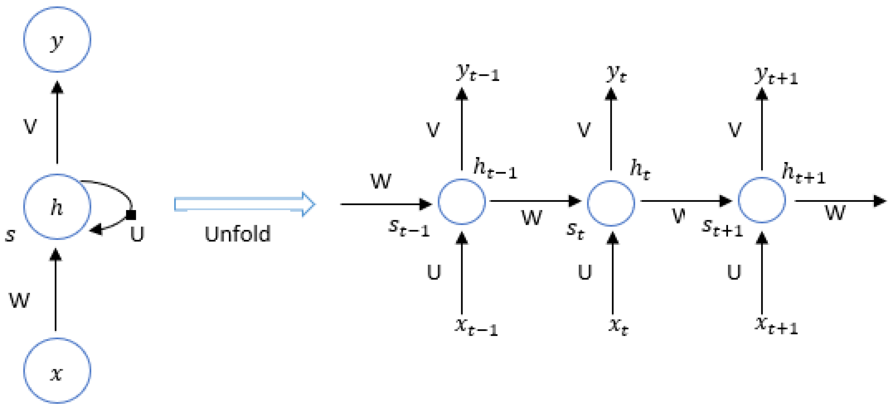
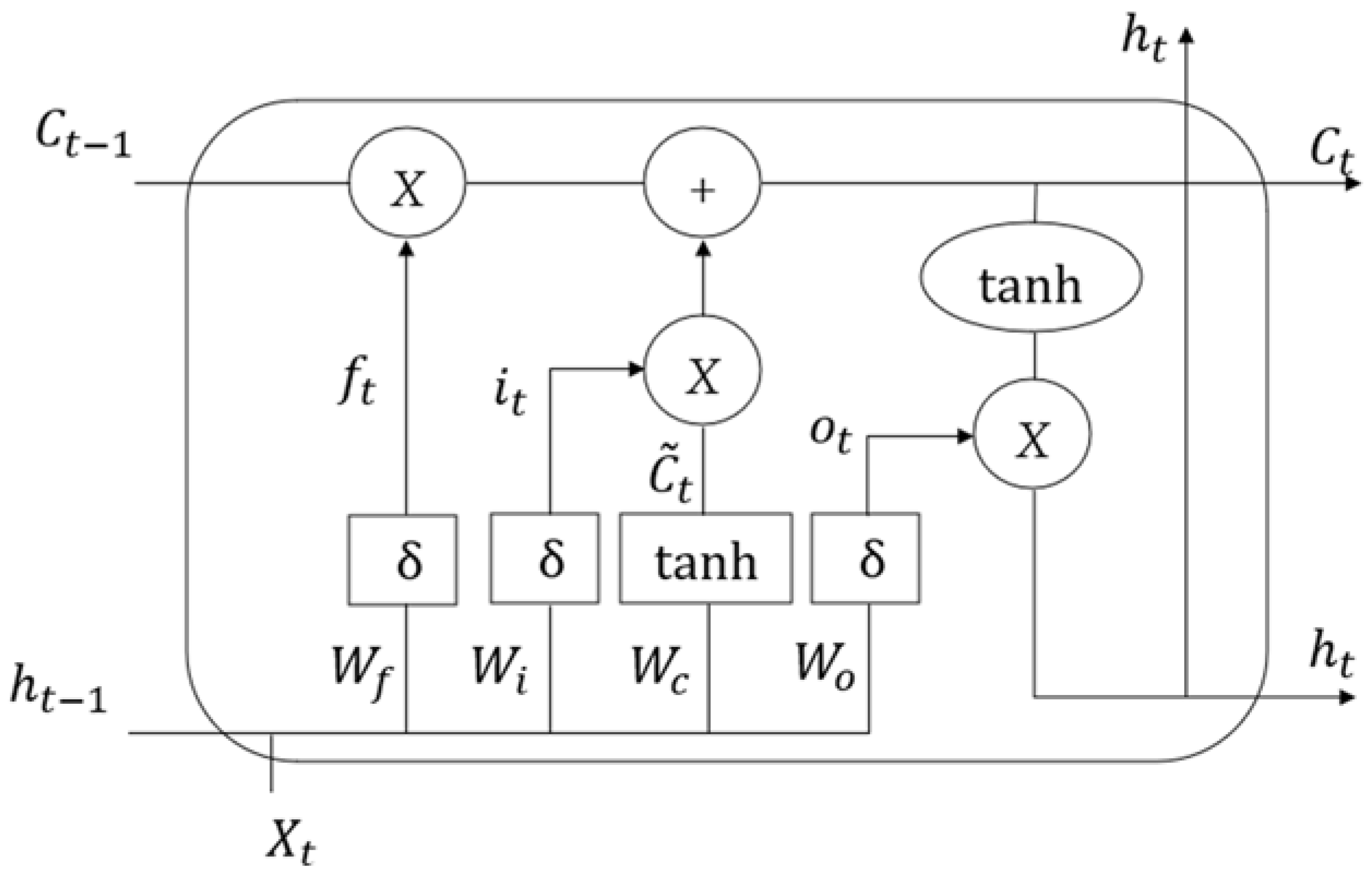
The Recurrent Neural Network Approach

Recurrent neural networks (RNN) are a framework for processing sequential data, remembering the previous information through the connection structure between each layer and using this information to influence the output of later nodes. RNNs can fully exploit the temporal and semantic information in sequential data, and this approach is more capable of deeper representation than full connected neural networks and CNNs in processing temporal data. A typical recurrent neural network structure is shown in Figure 6. For ease of understanding, the RNN structure in Figure 6 is expanded dutifully in a time series as shown in Figure 7. It is worth noting that the nodes in the recurrent layer of the RNN represent a hidden layer state rather than a neuron.

In Figure 7, $\mathrm{x}$ represents the inputs, $\mathrm{h}$ represents the hidden layer output, and $\mathrm{y}$ represents the output layer output. The right-hand side of Figure 7 is the form of an RNN expanded on the time axis, where the input is a time series $\left\{\cdots {,\mathrm{x}}_{\mathrm{t}-1}{,\mathrm{x}}_{\mathrm{t}}{,\mathrm{x}}_{\mathrm{t}+1},\cdots \right\}$, where ${\mathrm{x}}_{\mathrm{t}}\in {\mathrm{R}}^{\mathrm{n}}$ and $\mathrm{n}$ is the number of neurons in the input layer. Correspondingly, the hidden layer is $\left\{\cdots {,\mathrm{h}}_{\mathrm{t}-1}{,\mathrm{h},\mathrm{h}}_{\mathrm{t}+1},\cdots \right\}$, where ${\mathrm{h}}_{\mathrm{t}}\in {\mathrm{R}}^{\mathrm{m}}$ and $\mathrm{m}$ is the number of neurons in the hidden layer. The output value $\mathrm{y}$ at the moment $\mathrm{t}$ is not only influenced by the input $\mathrm{x}$ at the same moment, but also by the state of the hidden layer $\mathrm{s}$ at the previous moment. Such feedback is called ‘memory’ or ‘state’ $\mathrm{s}$ in RNN and is at the heart of it. This leads to the following computational process for the RNN model. The hidden layer calculation formula can be expressed as:

$${\mathrm{h}}_{\mathrm{t}}{=\mathrm{f}}_{\mathrm{h}}\left({\mathrm{s}}_{\mathrm{t}}\right)$$

(37)

where,

$${\mathrm{s}}_{\mathrm{t}}{=\mathrm{Wx}}_{\mathrm{t}}{+\mathrm{Uh}}_{\mathrm{t}-1}{+\mathrm{b}}_{\mathrm{h}}$$

(38)

${\mathrm{f}}_{\mathrm{h}}$ represents the activation function of the hidden layer, ${\mathrm{b}}_{\mathrm{h}}$ represents the bias of the hidden layer, $\mathrm{W}$ is the weight matrix from the input layer to the hidden layer, $\mathrm{U}$ is the weight matrix from the hidden layer outputs at time $\mathrm{t}-1$ to the hidden layer outputs at time $\mathrm{t}$, ${\mathrm{s}}_{\mathrm{t}}$ represent the state of the neuron at moments $\mathrm{t}$, and ${\mathrm{h}}_{\mathrm{t}-1}$ represents the output of the hidden layer at the previous moment.

The RNN outputs are $\left\{\cdots {,\mathrm{y}}_{\mathrm{t}-1}{,\mathrm{y},\mathrm{y}}_{\mathrm{t}+1},\cdots \right\}$, where ${\mathrm{y}}_{\mathrm{t}}\in {\mathrm{R}}^{\mathrm{p}}$ with $\mathrm{p}$ being the number of neurons in the output layer. The output layer is a fully connected layer, which means that each neuron in the hidden layer is connected to all the neurons in the output layer, and the output layer expression is:

$${\mathrm{y}}_{\mathrm{t}}{=\mathrm{f}}_{\mathrm{o}}\left({\mathrm{Vh}}_{\mathrm{t}}{+\mathrm{b}}_{\mathrm{o}}\right)$$

(39)

where $\mathrm{V}$ is the weight matrix from the hidden layer to the output layer, ${\mathrm{f}}_{\mathrm{o}}$ and ${\mathrm{b}}_{\mathrm{o}}$ represent the output layer activation function and bias respectively.

As with traditional neural networks, the training of the network pattern parameters is based on an error back-propagation algorithm. The difference is that the parameters of the recurrent neurons in the RNN are shared from moment to moment, and thus the calculation of the gradient relies on the gradient of all past moments. For this reason, the error back propagation algorithm in RNNs is also known as the back propagation through time (BPTT). In the following, the cross-entropy is considered as the loss function, the $\tan \mathrm{h}$ function is the hidden layer activation function and the final output of the RNN is $\mathrm{y}$, the state and output at time $\mathrm{t}$ are:

$${\mathrm{h}}_{\mathrm{t}}=\tan \mathrm{h}\left({\mathrm{s}}_{\mathrm{t}}\right)=\tan \mathrm{h}\left(\mathrm{W}\right)$$

(40)

$${\hat{\mathrm{y}}}_{\mathrm{t}}=\mathrm{softmax}\left(\mathrm{V}{\mathrm{s}}_{\mathrm{t}}\right)$$

(41)

For sequence training the loss function is:

$$\mathrm{E}(\mathrm{y},\hat{\mathrm{y}})=\sum _{\mathrm{t}=0}^{\mathrm{T}}{\mathrm{E}}_{\mathrm{t}}\left({\mathrm{y}}_{\mathrm{t}},{\hat{\mathrm{y}}}_{\mathrm{t}}\right)=-\sum _{\mathrm{t}=0}^{\mathrm{T}}{\mathrm{y}}_{\mathrm{t}}\log {\hat{\mathrm{y}}}_{\mathrm{t}}$$

(42)

where ${\mathrm{y}}_{\mathrm{t}}$ and ${\hat{\mathrm{y}}}_{\mathrm{t}}$ are the true output value and the model prediction at moment $\mathrm{t}$ respectively, is and ${\mathrm{E}}_{\mathrm{t}}$ is the cross-entropy at moment $\mathrm{t}$.

In recent years, there has been increasing interest in the use of RNNs for equipment condition monitoring [163,164,165,166,167]. Abed et al. [168] have implemented RNN successfully to the detection and classification of motor bearing faults. Using discrete wavelet transforms, fault features are extracted from the current and vibration signals of induction motors. Using orthogonal fuzzy neighborhood discriminant analysis (OFDNA), these characteristics are decreased further. OFDNA is then applied to acquire the most effective fault classification features. The RNN classifier uses these features as training and test sets to provide fault detection and diagnosis. The results shows that the RNN-based fault diagnosis approach can detect and classify induction motor bearing faults under various operating conditions. Li et al. predict the deterioration trend of rolling bearings by integrating RNN and reinforcement learning in [169]. The singular spectral entropy of the vibration signal is utilized to characterize the deterioration condition of the bearing, and the degradation trend is split into several stages by moving average noise reduction. The training and testing set for the RNN model is comprised of these phases. Then, reinforcement learning is employed at each stage to optimize the parameters of the RNN’s hidden layer. By comparing RNN with reinforcement learning to ELM, SVM, and the original RNN model, the results indicate that RNN with reinforcement learning surpasses the other approaches in terms of prediction accuracy and convergence speed.

As seen in the previous paragraph, RNNs have already made progress in the application of equipment condition monitoring. In practice, however, RNNs still have limits, most notably the disappearance or expansion of gradients when dealing with lengthy sequence issues. To solve this problem, a long short-term memory (LSTM) network structure containing memory units is proposed in [170]. A typical LSTM neural network cell is shown in Figure 8. Both LSTM and RNN are trained with similar parameters on the neural network structure, with the main difference being on the recurrent neuron nodes.

In Figure 8, ${\mathrm{h}}_{\mathrm{t}}$ is the hidden state, which represents short-term memory, and ${\mathrm{C}}_{\mathrm{t}}$ is the cell state, which represents long-term memory. Compared to the RNN basic recurrent neurons, the LSTM has an additional state or memory for long-term storage and another for short-term storage. The long-term state is updated slowly and mostly maintains long-term dependent information, whereas the short-term state is updated more often and varies more depending on the neuron’s current state. The LSTM additionally has three gated cyclic units to regulate the updating and forgetting of memories, ensuring that vital information is constantly remembered, and less significant information is discarded, hence permitting the storage and flow of memories in the hidden layer units.

In the recent decade, LSTM has received a great deal of interest in the field of equipment condition monitoring since it overcomes the limitations of RNNs in processing long sequences [81,171,172,173,174,175,176,177,178,179,180,181,182]. Regarding fault detection and diagnosis, Luo et al. [183] implemented fault detection for permanent magnet synchronous motor using LSTM. To train the LSTM model, the three-phase current values and rotor position data at the moment of continuous sampling are utilized as inputs, and the current value at the next sampling moment is used as the desired output. Detection of faults is then accomplished by monitoring the model’s prediction error. In [184], Xiao et al. propose a LSTM-based approach for fault diagnosis in three-phase asynchronous motors. Each type of vibration signal is first converted into a three-dimensional tensor sample matching to the current condition and utilized as input to the LSTM classifier to establish the link between the vibration signal and the fault condition. After testing the LSTM, linear regression (LR), SVM, multilayer neural network, and original RNN on six asynchronous motors with various failure circumstances, the LSTM demonstrated the highest classification accuracy at 98.28%. In [92], Bie et al. presented a model based on complete ensemble empirical model decomposition (CEEMD) and LSTM for fault diagnostics of reciprocating pumps. The vibration signal is processed using CEEMD and singular spectral entropy to generate feature vectors for fault diagnostics using an LSTM classifier. In comparison to traditional neural network approaches, the LSTM has the best classification accuracy. Regarding fault prognosis and remaining useful life (RUL) estimation, Lee et al. [185] utilized LSTM to estimate the RUL for gear pumps. Using the temporal and frequency domain features of the vibration signal obtained by signal analysis, the health index of the pump was characterized. The RUL estimate was then done using a Kalman filter to combine the health index and pressure data. Through training in a bi-directional LSTM model, it is able to predict the future of the RUL. Gate recurrent units (GRUs) were introduced by Cho et al. [186] due to the varying contributions of various gating to learning ability. By removing the gates with minor contributions and their related weights, the model simplifies the structure of the LSTM network and enhances the efficiency of learning. It consists of two gating units, the reset gate and the update gate. This method has also been used to the monitoring of equipment condition [187,188,189]. The reset gate acts similarly to the input gate of the LSTM unit, but the update gate implements the forgetting gate and output gate. Zhao et al. [190] proposed a hybrid strategy for machine condition monitoring that combines manual feature creation with automatic feature learning. First, time domain features are retrieved manually from the device signals and utilized as input to an improved bidirectional GRU network. This is followed by learning to represent faults using the GRU network’s produced local features. A supervised learning layer is then employed to predict the machine condition. The research demonstrates the efficacy and generalizability of the system through the prediction of tool wear, the diagnosis of gearbox faults, and the detection of early bearing faults.

The relevant references for the RNN methods discussed in this section are summarized in

Table 21. Motor condition monitoring using recurrent neural network.

References	Application	Type of Equipment	Signal	Fault Type
[163]	Fault detection and isolation	Induction motor	Current signal	Stator and bearing fault
[168]	Fault detection and diagnosis	Brushless DC motor	Current and vibration signal	Bearing fault (Ball, inner race, and outer race faults)
[171]	Fault diagnosis	Induction motor	Rotating sound signal	Bearing fault (Ball, inner race, and outer race faults)
[172]	Fault diagnosis	Induction motor	Vibration and current signal	Unbalance fault with different severity
[183]	Fault detection	Permanent Magnet Synchronous Motor	Three-phase current signal and rotor position information	open and shot circuit fault (instantaneous fault or gradual fault), and winding resistance increase or decrease (early faults)
[184]	Fault diagnosis	Three-phase asynchronous motor	Vibration signal	Voltage imbalance, rotor imbalance, faulty bearing, broken rotor bars, and bowed rotor
[186]	Remaining useful life prediction	Induction motor	Current and voltage signal	Bearing fault

,

Table 22. Pump condition monitoring using recurrent neural network.

References	Application	Type of Equipment	Signal	Fault Type
[164]	Modelling	Heat pump	Temperature	Clogging fault
[173]	Fault prognosis	Power pump	Multiple sensors monitoring data	N/A
[174]	Remaining useful life	Electromagnetic pump	Vibration and pressure signal	Cavitation
[175]	Future state prediction	Water injection pump	Multiple sensors monitoring data (vibration, temperature, flow, pressure, distance)	N/A
[92]	Fault diagnosis	Reciprocating pump	Vibration signal	Piston wear, bearing wear, and valve disc wear faults
[185]	Remaining useful life	Hydraulic gear pump	Vibration, flow, and pressure signal	Fuel contamination
[188]	State trend prediction	Aircraft pump	Accumulator pressure data	N/A
[81]	Fault prognosis	Reactor coolant pump	Shaft seal leakage flow	Seal leakage fault
[189]	Condition prediction	Main pump	Temperature and leakage flow	Bearing wear fault

and

Table 23. Bearing condition monitoring using recurrent neural network.

References	Application	Type of Equipment	Signal	Fault Type
[34]	Feature extraction	Rolling bearing	Vibration signal	Inner race, outer race, cage and ball faults
[165]	Fault prognosis	Rolling bearing	Vibration signal	Outer race fault
[169]	State trend prediction	Rolling bearing	Vibration signal	Inner race fault
[176]	Fault diagnosis	Rolling bearing	Vibration signal	Ball, inner race, and outer race faults
[177]	Fault diagnosis	Rolling bearing	Vibration signal	Ball, inner race, and outer race faults
[178]	Fault diagnosis	Rolling bearing	Vibration signal	Inner race, outer race and roller fault and combination of outer race and roller faults
[179]	Condition monitoring	Rolling bearing	Vibration signal	roller, inner race, and outer race fault
[180]	Fault prediction	Aero engine bearing	Vibration signal	Inner race, outer race, and ball faults
[181]	Remaining useful life	Rolling bearing	Vibration signal	Inner race, outer race, and ball faults
[187]	Fault diagnosis	Rolling bearing	Vibration signal	Inner race, outer race, and ball faults
[190]	Prognosis and remaining useful life prediction	Rolling bearing	Vibration signal	Inner race, outer race, and ball faults
[166]	Fault detection	Motor bearing	Current and vibration signal	Air gap eccentricity and ball faults
[167]	Fault diagnosis	Rolling bearing	Vibration signal	Inner race, outer race, and ball faults
[182]	Fault diagnosis	Rolling bearing	Vibration signal	Inner race, outer race, and ball faults

.

3. Conclusions

In this paper, we review the progress of the last 10 years of research into data-driven condition monitoring applied to three types of commonly industrial equipment: motors, pumps, and bearings. The structure and applications of data-driven condition monitoring are investigated. The large number of reviewed works indicate that data-driven condition monitoring of industrial equipment is gaining popularity. The reported data-driven equipment condition monitoring approaches generally involve a feature extraction phase and fault classification/prediction phase. The most widely used feature extraction techniques include Fourier Transform (FT), Wavelet Transform (WT), and Empirical Modal Decomposition (EMD). The most widely used classification and prediction techniques include artificial neural networks (ANN), support vector machines (SVM) and extreme learning machines (ELM), deep belief networks (DBN), convolutional neural networks (CNN) and recurrent neural networks (RNN).

As a result of the literature assessment shown above, the following list of unsolved critical future challenges is presented.

• Literature has focused on various types of faults, including rotor, stator winding, bearing wear, unbalance faults, etc., in motors; cavitation, leakage, impeller faults, etc., in pumps; and inner race, outer race, ball, and roller faults in bearings. These faults are often assessed individually in condition monitoring, however, multiple faults can exist in a single component, so it is necessary to consider this situation carefully and to achieve differentiation and resolution of multiple faults.
• As different types of equipment may have faults of varying severity in their operating condition, it is essential to consider the state of development of faults to correctly diagnose and detect them at the earliest stages of their occurrence, which is very rare in research work.
• Another issue that cannot be disregarded is the imbalance of data categories, since equipment always operates under normal conditions to collect normal data, resulting in a small number of fault sample data. In addition, most AI-based monitoring systems utilize historical or current databases. However, it is impossible to have a database for all machines operating under all conditions. Therefore, it is necessary to research how to allow AI models to execute condition monitoring in the absence of training data or under particular operating conditions that have not been trained.

References

1. Wang, W.; Taylor, J.; Rees, R.J. Recent Advancement of Deep Learning Applications to Machine Condition Monitoring Part 1: A Critical Review. Acoust. Aust. 2021, 49, 207–219. [Google Scholar] [CrossRef]
2. Alshorman, O.; Irfan, M.; Saad, N.; Zhen, D.; Haider, N.; Glowacz, A.; Alshorman, A. A Review of Artificial Intelligence Methods for Condition Monitoring and Fault Diagnosis of Rolling Element Bearings for Induction Motor. Shock Vib. 2021, 2020, 8843759. [Google Scholar] [CrossRef]
3. Drakaki, M.; Karnavas, Y.L.; Tziafettas, I.A.; Linardos, V.; Tzionas, P. Machine Learning and Deep Learning Based Methods Toward Industry 4.0 Predictive Maintenance in Induction Motors: A State of the Art Survey. J. Ind. Eng. Manag. 2022, 15, 31–57. [Google Scholar] [CrossRef]
4. Dash, R.N.; Sahu, S.; Panigrahi, C.K.; Subudhi, B. Condition monitoring of induction motors: A review. In Proceedings of the International Conference on Signal Processing, Communication, Power, and Embedded System (SCOPES), Paralakhemundi, India, 3–5 October 2016. [Google Scholar]
5. Gissella, J.; Lázaro, M.; Borrás Pinilla, C.; Prada, S.R. A survey of approaches for fault diagnosis in axial piston pumps. In Proceedings of the ASME International Mechanical Engineering Congress and Exposition, Proceedings (IMECE), Phoenix, AZ, USA, 11–17 November 2016. [Google Scholar]
6. Olesen, J.F.; Shaker, H.R. Predictive maintenance for pump systems and thermal power plants: State-of-the-art review, trends and challenges. Sensors 2020, 20, 24–25. [Google Scholar]
7. Cerrada, M.; Sánchez, R.V.; Li, C.; Pacheco, F.; Cabrera, D.; de Oliveira, J.V.; Vásquez, R.E. A review on data-driven fault severity assessment in rolling bearings. Mech. Syst. Signal Process. 2018, 99, 169–196. [Google Scholar] [CrossRef]
8. Nawab, S.; Quatieri, T.; Lim, J. Signal reconstruction from short-time Fourier transform magnitude. IEEE Trans. Acoust. Speech Signal Process. 1983, 31, 986–998. [Google Scholar] [CrossRef]
9. Daubechies, I. The wavelet transform, time-frequency localization and signal analysis. IEEE Trans. Inf. Theory 1990, 36, 961–1005. [Google Scholar] [CrossRef] [Green Version]
10. Huang, N.E.; Shen, Z.; Long, S.R.; Wu, M.C.; Shih, H.H.; Zheng, Q.; Yen, N.-C.; Tung, C.C.; Liu, H.H. The Empirical Mode Decomposition and the Hilbert Spectrum for Nonlinear and Non-Stationary Time Series Analysis. Proc. R. Soc. Lond. Ser. A Math. Phys. Eng. Sci. 1998, 454, 903–995. [Google Scholar] [CrossRef]
11. Jain, A.K.; Mao, J.; Mohiuddin, K.M. Artificial neural networks: A tutorial. Computer 1996, 3, 31–44. [Google Scholar] [CrossRef] [Green Version]
12. Cortes, C.; Vapnik, V. Support-vector networks. Mach. Learn. 1995, 20, 273–279. [Google Scholar] [CrossRef]
13. Huang, G.-B.; Zhu, Q.-Y.; Siew, C.-K. Extreme learning machine: Theory and applications. Neurocomputing 2006, 70, 489–501. [Google Scholar] [CrossRef]
14. Mohamed, A.-R.; Dahl, G.E.; Hinton, G. Acoustic Modeling Using Deep Belief Networks. IEEE Trans. Audio Speech Lang. Process. 2012, 20, 14–22. [Google Scholar] [CrossRef]
15. O’Shea, K.; Nash, R. An Introduction to Convolutional Neural Networks. arXiv 2015, arXiv:1511.08458. [Google Scholar]
16. Salehinejad, H.; Barfett, J.; Sankar, S.; Barfett, J.; Colak, E.; Valaee, S. Recent advances in recurrent neural networks. arXiv 2017, arXiv:1801.01078. [Google Scholar]
17. Abbasi, T.; Lim, K.H.; Soomro, T.A.; Ismail, I.; Ali, A. Condition Based Maintenance of Oil and Gas Equipment: A Review. In Proceedings of the 2020 3rd International Conference on Computing, Mathematics and Engineering Technologies (iCoMET), Sukkur, Pakistan, 29–30 January 2020. [Google Scholar]
18. Chen, X.; Wang, S.; Qiao, B.; Chen, Q. Basic research on machinery fault diagnostics: Past, present, and future trends. Front. Mech. Eng. 2018, 13, 264–291. [Google Scholar] [CrossRef] [Green Version]
19. Yang, Y.; Haque, M.M.M.; Bai, D.; Tang, W. Fault Diagnosis of Electric Motors Using Deep Learning Algorithms, and Its Application: A Review. Energies 2021, 14, 7017. [Google Scholar] [CrossRef]
20. Althubaiti, A.; Elasha, F.; Teixeira, J.A. Fault diagnosis and health management of bearings in rotating equipment based on vibration analysis—A review. J. Vibroeng. 2021, 24, 46–74. [Google Scholar] [CrossRef]
21. Khazaee, M.; Rezaniakolaie, A.; Moosavian, A.; Rosendahl, L. A novel method for autonomous remote condition monitoring of rotating machines using piezoelectric energy harvesting approach. Sens. Actuators A Phys. 2019, 95, 37–50. [Google Scholar] [CrossRef]
22. Atamuradov, V.; Medjaher, K.; Camci, F.; Zerhouni, N.; Dersin, P.; Lamoureux, B. Machine health indicator construction framework for failure diagnostics and prognostics. J. Signal Process. Syst. 2021, 92, 591–609. [Google Scholar] [CrossRef]
23. Wang, Y.; Wei, Z.; Yang, J. Feature Trend Extraction and Adaptive Density Peaks Search for Intelligent Fault Diagnosis of Machines. IEEE Trans. Ind. Inform. 2019, 15, 105–115. [Google Scholar] [CrossRef]
24. Luo, B.; Wang, H.; Liu, H.; Li, B.; Peng, F. Early Fault Detection of Machine Tools Based on Deep Learning and Dynamic Identification. IEEE Trans. Ind. Electron. 2019, 66, 509–518. [Google Scholar] [CrossRef]
25. Jiang, G.; He, H.; Yan, J.; Xie, P. Multiscale Convolutional Neural Networks for Fault Diagnosis of Wind Turbine Gearbox. IEEE Trans. Ind. Electron. 2019, 66, 3196–3207. [Google Scholar] [CrossRef]
26. Mustafa, D.; Yicheng, Z.; Minjie, G.; Jonas, H.; Jürgen, F. Motor Current Based Misalignment Diagnosis on Linear Axes with Short-Time Fourier Transform (STFT). Procedia CIRP 2022, 106, 239–243. [Google Scholar] [CrossRef]
27. Li, Y.; Feng, G.; Li, X.; Si, Q.; Zhu, Z. An experimental study on the cavitation vibration characteristics of a centrifugal pump at normal flow rate. J. Mech. Sci. Technol. 2018, 32, 4711–4720. [Google Scholar] [CrossRef]
28. Santhoshi, M.; Babu, K.; Kumar, S.; Nandan, D. An Investigation on Rolling Element Bearing Fault and Real-Time Spectrum Analysis by Using Short-Time Fourier Transform. In Proceedings of the International Conference on Recent Trends in Machine Learning, IoT, Smart Cities and Applications. Advances in Intelligent Systems and Computing, Telangana, India, 18 October 2021; Gunjan, V.K., Zurada, J.M., Eds.; Springer: Singapore, 2021. [Google Scholar]
29. Huang, W.; Gao, G.; Li, N.; Jiang, X.; Zhu, Z. Time-Frequency Squeezing and Generalized Demodulation Combined for Variable Speed Bearing Fault Diagnosis. IEEE Trans. Instrum. Meas. 2019, 68, 2819–2829. [Google Scholar] [CrossRef]
30. Mishra, N.; Roy, K.; Rautela, P. Investigation of Motor Faults in NPP Using in Service Motor Monitoring System. In Proceedings of the 2016 IEEE 1st International Conference on Power Electronics, Intelligent Control and Energy Systems (ICPEICES), Delhi, India, 4–6 July 2016. [Google Scholar]
31. Awadallah, M.A.; Morcos, M.M. Diagnosis of stator short circuits in brushless DC motors by monitoring phase Voltages. IEEE Trans. Energy Convers. 2005, 20, 246–247. [Google Scholar] [CrossRef]
32. Aimer, A.F.; Boudinar, A.H.; Benouzza, N.; Bendiabdellah, A. Simulation and experimental study of induction motor broken rotor bars fault diagnosis using stator current spectrogram. In Proceedings of the 2015 3rd International Conference on Control, Engineering & Information Technology (CEIT), Tlemcen, Algeria, 25–27 May 2015. [Google Scholar]
33. Gao, H.; Liang, L.; Chen, X.; Xu, G. Feature Extraction and Recognition for Rolling Element Bearing Fault Utilizing Short-Time Fourier Transform and Non-negative Matrix Factorization. Chin. J. Mech. Eng. 2014, 28, 96–105. [Google Scholar] [CrossRef]
34. He, M.; He, D. Deep Learning Based Approach for Bearing Fault Diagnosis. IEEE Trans. Ind. Appl. 2017, 53, 3057–3065. [Google Scholar] [CrossRef]
35. Zhao, W.; Wang, Z.; Ma, J.; Li, L. Fault Diagnosis of a Hydraulic Pump Based on the CEEMD-STFT Time-Frequency Entropy Method and Multiclass SVM Classifier. Shock Vib. 2016, 2016, 2609856. [Google Scholar] [CrossRef] [Green Version]
36. Chao, Q.; Wei, X.; Lei, J.; Tao, J.; Liu, C. Improving accuracy of cavitation severity recognition in axial piston pumps by denoising time–frequency images. Meas. Sci. Technol. 2022, 33, 055116. [Google Scholar] [CrossRef]
37. Tao, H.; Wang, P.; Chen, Y.; Stojanovic, V.; Yang, H. An unsupervised fault diagnosis method for rolling bearing using STFT and generative neural networks. J. Frankl. Inst. 2020, 357, 7286–7307. [Google Scholar] [CrossRef]
38. Wang, L.H.; Zhao, X.P.; Wu, J.X.; Xie, Y.Y.; Zhang, Y.H. Motor fault diagnosis based on short-time Fourier transform and convolutional neural network. Chin. J. Mech. Eng. 2017, 30, 1357–1368. [Google Scholar] [CrossRef]
39. Mostafavi, A.; Sadighi, A. A Novel Online Machine Learning Approach for Real-Time Condition Monitoring of Rotating Machines. In Proceedings of the 2021 9th RSI International Conference on Robotics and Mechatronics (ICRoM), Tehran, Iran, 17–19 November 2021. [Google Scholar]
40. Jami, A.; Heyns, P.S. Impeller fault detection under variable flow conditions based on three feature extraction methods and artificial neural networks. J. Mech. Sci. Technol. 2018, 32, 4079–4087. [Google Scholar] [CrossRef]
41. Siano, D.; Panza, M.A. Diagnostic method by using vibration analysis for pump fault detection. Energy Procedia 2018, 148, 10–17. [Google Scholar] [CrossRef]
42. Rauber, T.W.; Oliveira-Santos, T.; de Assis Boldt, F.; Rodrigues, A.; Varejao, F.M.; Ribeiro, M.P. Kernel and Random Extreme Learning Machine Applied to Submersible Motor Pump Fault Diagnosis. In Proceedings of the 2017 International Joint Conference on Neural Networks (IJCNN), Anchorage, AK, USA, 14–19 May 2017. [Google Scholar]
43. Kumar, K.V.; Raj, A.C.B. Static eccentricity failure diagnosis for induction machine using wavelet analysis. In Proceedings of the 2017 International Conference on Innovations in Green Energy and Healthcare Technologies (IGEHT), Coimbatore, India, 16–18 March 2017. [Google Scholar]
44. Huo, Z.; Zhang, Y.; Francq, P.; Shu, L.; Huang, J. Incipient Fault Diagnosis of Roller Bearing Using Optimized Wavelet Transform Based Multi-Speed Vibration Signatures. IEEE Access 2017, 5, 19442–19456. [Google Scholar] [CrossRef] [Green Version]
45. Siddiqui, K.M.; Giri, V.K. Broken rotor bar fault detection in induction motors using Wavelet Transform. In Proceedings of the 2012 International Conference on Computing, Electronics and Electrical Technologies (ICCEET), Nagercoil, India, 21–22 March 2012. [Google Scholar]
46. Konar, P.; Chattopadhyay, P. Bearing fault detection of induction motor using wavelet and Support Vector Machines (SVMs). Appl. Soft Comput. 2011, 11, 4203–4211. [Google Scholar] [CrossRef]
47. Cheng, Y.; Lin, M.; Wu, J.; Zhu, H.; Shao, X. Intelligent fault diagnosis of rotating machinery based on continuous wavelet transform-local binary convolutional neural network. Knowl. Based Syst. 2021, 216, 106796. [Google Scholar] [CrossRef]
48. Lee, I.-S. Fault Diagnosis Of Induction Motors Using Discrete Wavelet Transform And Artificial Neural Network. In Communications in Computer and Information Science, Proceedings of the International Conference on Human-Computer Interaction, Orlando, FL, USA, 9–14 July 2011; Springer: Berlin/Heidelberg, Germany, 2011. [Google Scholar]
49. Heydarzadeh, M.; Zafarani, M.; Nourani, M.; Akin, B. A Wavelet-Based Fault Diagnosis Approach for Permanent Magnet Synchronous Motors. IEEE Trans. Energy Convers. 2019, 34, 761–772. [Google Scholar] [CrossRef]
50. Surti, K.V.; Naik, C.A. Bearing Condition Monitoring of Induction Motor Based on Discrete Wavelet Transform & K-nearest Neighbor. In Proceedings of the 2018 3rd International Conference for Convergence in Technology (I2CT), Pune, India, 6–8 April 2018. [Google Scholar]
51. Li, B.; Xia, H. Research on feature recognition of nuclear power equipment based on the optimal wavelet basis. In Proceedings of the International Conference on Nuclear Engineering, Chengdu, China, 29 July–2 August 2013; American Society of Mechanical Engineers: New York, NY, USA, 2013; Volume 55829. [Google Scholar]
52. Zheng, Z.; Wang, Z.; Zhu, Y.; Tang, S.; Wang, B. Feature extraction method for hydraulic pump fault signal based on improved empirical wavelet transform. Processes 2019, 7, 824. [Google Scholar] [CrossRef] [Green Version]
53. Muralidharan, V.; Sugumaran, V. Feature extraction using wavelets and classification through decision tree algorithm for fault diagnosis of mono-block centrifugal pump. Measurement 2013, 46, 353–359. [Google Scholar] [CrossRef]
54. Xu, Y.; Li, Z.; Wang, S.; Li, W.; Sarkodie-Gyan, T.; Feng, S. A hybrid deep-learning model for fault diagnosis of rolling bearings. Measurement 2021, 169, 108502. [Google Scholar] [CrossRef]
55. Tang, S.; Zhu, Y.; Yuan, S. An improved convolutional neural network with an adaptable learning rate towards multi-signal fault diagnosis of hydraulic piston pump. Adv. Eng. Inform. 2021, 50, 101406. [Google Scholar] [CrossRef]
56. Kamiel, B.; McKee, K.; Entwistle, R.; Mazhar, I.; Howard, I. Multi Fault Diagnosis of the Centrifugal Pump Using the Wavelet Transform and Principal Component Analysis. In Proceedings of the 9th IFToMM International Conference on Rotor Dynamics, Milan, Italy, 22–25 September 2014; Springer: Cham, Switzerland, 2015. [Google Scholar]
57. Al Tobi, M.; Bevan, G.; Wallace, P.; Harrison, D.K.; Okedu, K. Faults diagnosis of a centrifugal pump using multilayer perceptron genetic algorithm back propagation and support vector machine with discrete wavelet transform-based feature extraction. Comput. Intell. 2021, 37, 21–46. [Google Scholar] [CrossRef]
58. Chen, J.; Pan, J.; Li, Z.; Zi, Y.; Chen, X. Generator bearing fault diagnosis for wind turbine via empirical wavelet transform using measured vibration signals. Renew. Energy 2016, 89, 80–92. [Google Scholar] [CrossRef]
59. Eren, L.; Cekic, Y.; Devaney, M.J. Motor Condition Monitoring by Empirical Wavelet Transform. In Proceedings of the 2018 26th European Signal Processing Conference (EUSIPCO), Rome, Italy, 3–7 September 2018. [Google Scholar]
60. Ebrahimi, B.M.; Roshtkhari, M.J.; Faiz, J.; Khatami, S.V. Advanced Eccentricity Fault Recognition in Permanent Magnet Synchronous Motors Using Stator Current Signature Analysis. IEEE Trans. Ind. Electron. 2014, 61, 2041–2052. [Google Scholar] [CrossRef]
61. Bordoloi, D.; Tiwari, R. Identification of suction flow blockages and casing cavitations in centrifugal pumps by optimal support vector machine techniques. J. Braz. Soc. Mech. Sci. Eng. 2017, 39, 2957–2968. [Google Scholar] [CrossRef]
62. Ding, Y.; Ma, L.; Wang, C.; Tao, L. An EWT-PCA and Extreme Learning Machine Based Diagnosis Approach for Hydraulic Pump. IFAC-PapersOnLine 2020, 53, 43–47. [Google Scholar] [CrossRef]
63. Islam, M.M.; Kim, J.M. Automated bearing fault diagnosis scheme using 2D representation of wavelet packet transform and deep convolutional neural network. Comput. Ind. 2019, 106, 142–153. [Google Scholar] [CrossRef]
64. Ding, X.; He, Q. Energy-Fluctuated Multiscale Feature Learning with Deep ConvNet for Intelligent Spindle Bearing Fault Diagnosis. IEEE Trans. Instrum. Meas. 2017, 66, 1926–1935. [Google Scholar] [CrossRef]
65. Wu, Z.; Huang, N. Ensemble Empirical Mode Decomposition: A Noise-Assisted Data Analysis Method. Adv. Adapt. Data Anal. 2009, 1, 1–41. [Google Scholar] [CrossRef]
66. Antonino-Daviu, J.A.; Riera-Guasp, M.; Pons-Llinares, J.; Roger-Folch, J.; Pérez, R.B.; Charlton-Pérez, C. Toward Condition Monitoring of Damper Windings in Synchronous Motors via EMD Analysis. IEEE Trans. Energy Convers. 2012, 27, 432–439. [Google Scholar] [CrossRef]
67. Lu, C.; Wang, S.; Zhang, C. Fault diagnosis of hydraulic piston pumps based on a two-step EMD method and fuzzy C-means clustering. Proc. Inst. Mech. Eng. Part C J. Mech. Eng. Sci. 2016, 230, 2913–2928. [Google Scholar] [CrossRef]
68. Jiao, X.; Jing, B.; Huang, Y.; Li, J.; Xu, G. Research on fault diagnosis of airborne fuel pump based on EMD and probabilistic neural networks. Microelectron. Reliab. 2017, 75, 296–308. [Google Scholar] [CrossRef]
69. Zheng, J.; Cheng, J.; Yang, Y. Generalized empirical mode decomposition and its applications to rolling element bearing fault diagnosis. Mech. Syst. Signal Process. 2013, 40, 136–153. [Google Scholar] [CrossRef]
70. Dybała, J.; Zimroz, R. Rolling bearing diagnosing method based on empirical mode decomposition of machine vibration signal. Appl. Acoust. 2014, 77, 195–203. [Google Scholar] [CrossRef]
71. Mahmud, M.; Wang, W. A Smart Sensor-Based cEMD Technique for Rotor Bar Fault Detection in Induction Motors. IEEE Trans. Instrum. Meas. 2021, 70, 3523811. [Google Scholar] [CrossRef]
72. Li, S.; Ma, J. Early Fault Feature Extraction of Nuclear Main Pump Based on MEMD-1.5 Dimensional Teager Energy Spectrum. In Proceedings of the 2020 IEEE 9th Data Driven Control and Learning Systems Conference (DDCLS), Liuzhou, China, 20–22 November 2020. [Google Scholar]
73. Feng, Y.; Li, X.; Ke, Z.; Chen, Z.; Tao, M. Pump Bearing Fault Detection Based on EMD and SVM. In Proceedings of the 2018 26th International Conference on Nuclear Engineering, London, UK, 22–26 July 2018. [Google Scholar]
74. Tang, H.; Wu, Y.; Hua, G.; Ma, C. Fault diagnosis of pump using EMD and envelope spectrum analysis. J. Vib. Shock 2012, 31, 44–48. [Google Scholar]
75. Faiz, J.; Ghorbanian, V.; Ebrahimi, B.M. EMD-Based Analysis of Industrial Induction Motors with Broken Rotor Bars for Identification of Operating Point at Different Supply Modes. IEEE Trans. Ind. Inform. 2014, 10, 957–966. [Google Scholar] [CrossRef]
76. Sadeghi, R.; Samet, H.; Ghanbari, T. Detection of Stator Short-Circuit Faults in Induction Motors Using the Concept of Instantaneous Frequency. IEEE Trans. Ind. Inform. 2019, 15, 4506–4515. [Google Scholar] [CrossRef]
77. Liu, Z.; Liu, Y.; Shan, H.; Cai, B.; Huang, Q. A fault diagnosis methodology for gear pump based on EEMD and Bayesian network. PLoS ONE 2015, 10, e0125703. [Google Scholar] [CrossRef]
78. Lei, Y.; He, Z.; Zi, Y. EEMD method and WNN for fault diagnosis of locomotive roller bearings. Expert Syst. Appl. 2011, 38, 7334–7341. [Google Scholar] [CrossRef]
79. Zhang, X.; Liang, Y.; Zhou, J. A novel bearing fault diagnosis model integrated permutation entropy, ensemble empirical mode decomposition and optimized SVM. Measurement 2015, 69, 164–179. [Google Scholar] [CrossRef]
80. Li, H.; Liu, T.; Wu, X.; Chen, Q. Application of EEMD and improved frequency band entropy in bearing fault feature extraction. ISA Trans. 2019, 88, 170–185. [Google Scholar] [CrossRef] [PubMed]
81. Nguyen, H.P.; Baraldi, P.; Zio, E. Ensemble empirical mode decomposition and long short-term memory neural network for multi-step predictions of time series signals in nuclear power plants. Appl. Energy 2021, 283, 116346. [Google Scholar] [CrossRef]
82. Rui, X.; Liu, J.; Li, Y.; Qi, L.; Li, G. Research on fault diagnosis and state assessment of vacuum pump based on acoustic emission sensors. Rev. Sci. Instrum. 2020, 91, 025107. [Google Scholar] [CrossRef]
83. Lu, Y.; Xie, R.; Liang, S.Y. CEEMD-assisted kernel support vector machines for bearing diagnosis. Int. J. Adv. Manuf. Technol. 2020, 106, 3063–3070. [Google Scholar] [CrossRef]
84. Lu, C.; Wang, S.; Makis, V. Fault severity recognition of aviation piston pump based on feature extraction of EEMD paving and optimized support vector regression model. Aerosp. Sci. Technol. 2017, 67, 105–117. [Google Scholar] [CrossRef]
85. Zhao, H.; Sun, M.; Deng, W.; Yang, X. A New Feature Extraction Method Based on EEMD and Multi-Scale Fuzzy Entropy for Motor Bearing. Entropy 2017, 19, 14. [Google Scholar] [CrossRef] [Green Version]
86. Torres, M.E.; Colominas, M.A.; Schlotthauer, G.; Flandrin, P. A Complete Ensemble Empirical Mode Decomposition with Adaptive Noise. In Proceedings of the 2011 IEEE International Conference on Acoustics, Speech and Signal Processing (ICASSP), Prague, Czech Republic, 22–27 May 2011. [Google Scholar]
87. Delgado-Arredondo, P.A.; Morinigo-Sotelo, D.; Osornio-Rios, R.A.; Avina-Cervantes, J.G.; Rostro-Gonzalez, H.; de Jesus Romero-Troncoso, R. Methodology for fault detection in induction motors via sound and vibration signals. Mech. Syst. Signal Process. 2017, 83, 568–589. [Google Scholar] [CrossRef]
88. Ke, Z.; Di, C.; Bao, X. Adaptive Suppression of Mode Mixing in CEEMD Based on Genetic Algorithm for Motor Bearing Fault Diagnosis. IEEE Trans. Magn. 2022, 58, 8200706. [Google Scholar] [CrossRef]
89. Refaat, S.S.; Abu-Rub, H.; Saad, M.S.; Aboul-Zahab, E.M.; Iqbal, A. ANN-Based for Detection, Diagnosis the Bearing Fault for Three Phase Induction Motors Using Current Signal. In Proceedings of the 2013 IEEE International Conference on Industrial Technology (ICIT), Cape Town, South Africa, 25–28 February 2013. [Google Scholar]
90. Shifat, T.A.; Hur, J.W. ANN Assisted Multi Sensor Information Fusion for BLDC Motor Fault Diagnosis. IEEE Access 2021, 9, 9429–9441. [Google Scholar] [CrossRef]
91. Li, Z.; Jiang, W.; Zhang, S.; Sun, Y.; Zhang, S. A Hydraulic Pump Fault Diagnosis Method Based on the Modified Ensemble Empirical Mode Decomposition and Wavelet Kernel Extreme Learning Machine Methods. Sensors 2021, 21, 2599. [Google Scholar] [CrossRef] [PubMed]
92. Bie, F.; Du, T.; Lyu, F.; Pang, M.; Guo, Y. An Integrated Approach Based on Improved CEEMDAN and LSTM Deep Learning Neural Network for Fault Diagnosis of Reciprocating Pump. IEEE Access 2021, 9, 23301–23310. [Google Scholar] [CrossRef]
93. Jigyasu, R.; Mathew, L.; Sharma, A. Multiple Faults Diagnosis of Induction Motor Using Artificial Neural Network. In Proceedings of the 2018 Second International Conference (ICAICR), Shimla, India, 14–15 July 2018. [Google Scholar]
94. Matveev, S.A.; Testoedov, N.A.; Vasil’kov, D.V.; Shirobokov, O.V.; Nadezhin, M.I. Methods for Diagnosing the Technical Condition of Spacecraft Electric Pump Units and Predicting Their Remaining Useful Life. Russ. Aeronaut. 2020, 63, 561–567. [Google Scholar] [CrossRef]
95. Gana, M.; Achour, H.; Belaid, K.; Chelli, Z.; Laghrouche, M.; Chaouchi, A. Non-invasive intelligent monitoring system for fault detection in induction motor based on lead-free-piezoelectric sensor using ANN. Meas. Sci. Technol. 2022, 33, 065105. [Google Scholar] [CrossRef]
96. Rahmawati, P.; Prajitno, P. Online Vibration Monitoring of a Water Pump Machine to Detect Its Malfunction Components Based on Artificial Neural Network. In Proceedings of the International Conference on Theoretical and Applied Physics, Yogyakarta, Indonesia, 6–8 September 2017. [Google Scholar]
97. Tian, Z.; Wong, L.; Safaei, N. A neural network approach for remaining useful life prediction utilizing both failure and suspension histories. Mech. Syst. Signal Process. 2010, 24, 1542–1555. [Google Scholar] [CrossRef]
98. Kumbhar, S.G.; Desavale, R.G.; Dharwadkar, N.V. Fault size diagnosis of rolling element bearing using artificial neural network and dimension theory. Neural Comput. Appl. 2021, 33, 16079–16093. [Google Scholar] [CrossRef]
99. Wang, A.; Li, Y.; Yao, Z.; Zhong, C.; Xue, B.; Guo, Z. A Novel Hybrid Model for the Prediction and Classification of Rolling Bearing Condition. Appl. Sci. 2022, 12, 3854. [Google Scholar] [CrossRef]
100. He, P.; Liu, C.; Ai, Q. Research on Reactor Coolant Pump Fault Diagnosis Method Based on Multi-Sensor Data Fusion. In Proceedings of the 2013 21st International Conference on Nuclear Engineering, Chengdu, China, 29 July–2 August 2013. [Google Scholar]
101. Haroun, S.; Nait Seghir, A.; Touati, S. Stator Inter Turn Fault and Voltage Unbalance Detection and Discrimination Approach for an Reactor Coolant Pump. In Proceedings of the 3rd International Conference on Systems and Control, Algiers, Algeria, 29–31 October 2013. [Google Scholar]
102. Shen, J.; Li, H.; Huang, L.; Mao, X.; Sheng, Z. Study on Online Monitoring of Equipment Condition Based on Local Outlier Factor and Artificial Neural Networks Model. Nucl. Power Eng. 2021, 42, 160–166. [Google Scholar]
103. Patel, R.K.; Giri, V.K. ANN based performance evaluation of BDI for condition monitoring of induction motor bearings. J. Inst. Eng. Ser. B 2017, 98, 267–274. [Google Scholar] [CrossRef]
104. Sharma, A.; Jigyasu, R.; Mathew, L.; Chatterji, S. Bearing Fault Diagnosis Using Frequency Domain Features and Artificial Neural Networks. In Proceedings of the Information and Communication Technology for Intelligent Systems, Ahmedabad, India, 6–7 April 2019. [Google Scholar]
105. Sheikh, M.A.; Nor, N.M.; Ibrahim, T.; Bakhsh, S.T.; Irfan, M.; Saad, N.B. An intelligent automated method to diagnose and segregate induction motor faults. J. Electr. Syst. 2017, 13, 241–254. [Google Scholar]
106. Bangalore, P.; Tjernberg, L.B. An Artificial Neural Network Approach for Early Fault Detection of Gearbox Bearings. IEEE Trans. Smart Grid 2015, 6, 980–987. [Google Scholar] [CrossRef]
107. Verma, A.K.; Sarangi, S.; Kolekar, M. Misalignment faults detection in an induction motor based on multi-scale entropy and artificial neural network. Electr. Power Compon. Syst. 2016, 44, 916–927. [Google Scholar] [CrossRef]
108. Sharma, R.; Pandey, N. A Neural Network Model for Electric Submersible Pump Surveillance. In Proceedings of the 2016 International Conference on Communication and Signal Processing (ICCSP), Melmaruvathur, India, 6–8 April 2016. [Google Scholar]
109. Patel, R.A.; Bhalja, B.R. Condition monitoring and fault diagnosis of induction motor using support vector machine. Electr. Power Compon. Syst. 2016, 44, 683–692. [Google Scholar] [CrossRef]
110. Wandekokem, E.; Mendel, E.; Fabris, F.; Valentim, M.; Batista, R.; Varejão, F.; Rauber, T. Diagnosing multiple faults in oil rig motor pumps using support vector machine classifier ensembles. Integr. Comput. Aided Eng. 2011, 18, 61–74. [Google Scholar] [CrossRef]
111. Xue, H.; Li, Z.; Wang, H.; Chen, P. Intelligent diagnosis method for centrifugal pump system using vibration signal and support vector machine. Shock Vib. 2014, 2014, 407570. [Google Scholar] [CrossRef]
112. Ahmad, Z.; Rai, A.; Maliuk, A.S.; Kim, J.M. Discriminant Feature Extraction for Centrifugal Pump Fault Diagnosis. IEEE Access 2020, 8, 165512–165528. [Google Scholar] [CrossRef]
113. Zhang, X.; Zhou, J. Multi-fault diagnosis for rolling element bearings based on ensemble empirical mode decomposition and optimized support vector machines. Mech. Syst. Signal Process. 2013, 41, 127–140. [Google Scholar] [CrossRef]
114. Cui, M.; Wang, Y.; Lin, X.; Zhong, M. Fault Diagnosis of Rolling Bearings Based on an Improved Stack Autoencoder and Support Vector Machine. IEEE Sens. J. 2021, 21, 4927–4937. [Google Scholar] [CrossRef]
115. Liming, Z.; Qi, C.; Xinwen, Z. Evaluation of Nuclear Equipment Technical Condition Based on Support Vector Machine. In Proceedings of the 2011 International Conference on Consumer Electronics, Communications and Networks (CECNet), Xianning, China, 16–18 April 2011. [Google Scholar]
116. Liu, J.; Seraoui, R.; Vitelli, V.; Zio, E. Nuclear power plant components condition monitoring by probabilistic support vector machine. Ann. Nucl. Energy 2013, 56, 23–33. [Google Scholar] [CrossRef] [Green Version]
117. Yu, R.; Li, X.; Tao, M.; Ke, Z. Fault Diagnosis of Feedwater Pump in Nuclear Power Plants Using Parameter-Optimized Support Vector Machine. In Proceedings of the International Conference on Nuclear Engineering, Charlotte, NC, USA, 26–30 June 2016. [Google Scholar]
118. Gangsar, P.; Tiwari, R. A support vector machine based fault diagnostics of Induction motors for practical situation of multi-sensor limited data case. Measurement 2019, 135, 694–711. [Google Scholar] [CrossRef]
119. Panda, A.K.; Rapur, J.S.; Tiwari, R. Prediction of flow blockages and impending cavitation in centrifugal pumps using Support Vector Machine (SVM) algorithms based on vibration measurements. Measurement 2018, 130, 44–56. [Google Scholar] [CrossRef]
120. Senanayaka, J.S.L.; Kandukuri, S.T.; Van Khang, H.; Robbersmyr, K.G. Early detection and classification of bearing faults using support vector machine algorithm. In Proceedings of the 2017 IEEE Workshop on Electrical Machines Design, Control and Diagnosis (WEMDCD), Nottingham, UK, 20–21 April 2017. [Google Scholar]
121. Gangsar, P.; Tiwari, R. Comparative investigation of vibration and current monitoring for prediction of mechanical and electrical faults in induction motor based on multiclass-support vector machine algorithms. Mech. Syst. Signal Process. 2017, 94, 464–481. [Google Scholar] [CrossRef]
122. Jiang, W.; Li, Z.; Li, J.; Zhu, Y.; Zhang, P. Study on a Fault Identification Method of the Hydraulic Pump Based on a Combination of Voiceprint Characteristics and Extreme Learning Machine. Processes 2019, 7, 894. [Google Scholar] [CrossRef] [Green Version]
123. Mao, W.; He, L.; Yan, Y.; Wang, J. Online sequential prediction of bearings imbalanced fault diagnosis by extreme learning machine. Mech. Syst. Signal Process. 2018, 83, 450–473. [Google Scholar] [CrossRef]
124. Mao, W.; He, J.; Li, Y.; Yan, Y. Bearing fault diagnosis with auto-encoder extreme learning machine: A comparative study. Proc. Inst. Mech. Eng. Part C J. Mech. Eng. Sci. 2017, 231, 1560–1578. [Google Scholar] [CrossRef]
125. Zheng, J.; Dong, Z.; Pan, H.; Ni, Q.; Liu, T.; Zhang, J. Composite multi-scale weighted permutation entropy and extreme learning machine based intelligent fault diagnosis for rolling bearing. Measurement 2019, 143, 69–80. [Google Scholar] [CrossRef]
126. Sharma, S.; Hasmat, M.; Ajay, K. External Fault Classification Experienced by Three-Phase Induction Motor Based on Multi-Class ELM. Procedia Comput. Sci. 2015, 70, 814–820. [Google Scholar] [CrossRef] [Green Version]
127. Lan, Y.; Hu, J.; Huang, J.; Niu, L.; Zeng, X.; Xiong, X.; Wu, B. Fault Diagnosis on Slipper Abrasion of Axial Piston Pump based on Extreme Learning Machine. Measurement 2018, 124, 378–385. [Google Scholar] [CrossRef]
128. Shao, H.; Jiang, H.; Li, X.; Wu, S. Intelligent fault diagnosis of rolling bearing using deep wavelet auto-encoder with extreme learning machine. Knowl. Based Syst. 2018, 140, 1–14. [Google Scholar]
129. Tamilselvan, P.; Wang, P. Failure diagnosis using deep belief learning based health state classification. Reliab. Eng. Syst. Saf. 2013, 115, 124–135. [Google Scholar] [CrossRef]
130. Shao, S.Y.; Sun, W.J.; Yan, R.Q.; Wang, P.; Gao, R. A deep learning approach for fault diagnosis of induction motors in manufacturing. Chin. J. Mech. Eng. 2017, 30, 1347–1356. [Google Scholar] [CrossRef] [Green Version]
131. Ma, S.; Chu, F. Ensemble deep learning-based fault diagnosis of rotor bearing systems. Comput. Ind. 2019, 105, 143–152. [Google Scholar] [CrossRef]
132. Shao, S.; Sun, W.; Wang, P.; Gao, R.X.; Yan, R. Learning Features from Vibration Signals for Induction Motor Fault Diagnosis. In Proceedings of the 2016 International Symposium on Flexible Automation (ISFA), Cleveland, OH, USA, 1–3 August 2016. [Google Scholar]
133. Wang, S.; Xiang, J.; Zhong, Y.; Tang, H. A data indicator-based deep belief networks to detect multiple faults in axial piston pumps. Mech. Syst. Signal Process. 2018, 112, 154–170. [Google Scholar] [CrossRef]
134. Tao, J.; Liu, Y.; Yang, D. Bearing fault diagnosis based on deep belief network and ultisensory information fusion. Shock Vib. 2016, 2016, 9306205. [Google Scholar]
135. Zou, Y.; Zhang, Y.; Mao, H. Fault diagnosis on the bearing of traction motor in high-speed trains based on deep learning. Alex. Eng. J. 2021, 60, 1209–1219. [Google Scholar] [CrossRef]
136. Shao, H.; Jiang, H.; Li, X.; Liang, T. Rolling bearing fault detection using continuous deep belief network with locally linear embedding. Comput. Ind. 2018, 96, 27–39. [Google Scholar] [CrossRef]
137. Shao, H.; Jiang, H.; Wang, F.; Wang, Y. Rolling bearing fault diagnosis using adaptive deep belief network with dual-tree complex wavelet packet. ISA Trans. 2017, 69, 187–201. [Google Scholar] [CrossRef]
138. Chen, Z.; Li, W. Multisensor Feature Fusion for Bearing Fault Diagnosis Using Sparse Autoencoder and Deep Belief Network. IEEE Trans. Instrum. Meas. 2017, 66, 1693–1702. [Google Scholar] [CrossRef]
139. Shao, H.; Jiang, H.; Zhang, X.; Niu, M. Rolling bearing fault diagnosis using an optimization deep belief network. Meas. Sci. Technol. 2015, 26, 115002. [Google Scholar] [CrossRef]
140. Shao, H.; Jiang, H.; Zhang, H.; Liang, T. Electric Locomotive Bearing Fault Diagnosis Using a Novel Convolutional Deep Belief Network. IEEE Trans. Ind. Electron. 2018, 65, 2727–2736. [Google Scholar] [CrossRef]
141. Zhao, H.; Yang, X.; Chen, B.; Chen, H.; Deng, W. Bearing fault diagnosis using transfer learning and optimized deep belief network. Meas. Sci. Technol. 2022, 33, 065009. [Google Scholar] [CrossRef]
142. Yu, K.; Lin, T.R.; Tan, J. A bearing fault and severity diagnostic technique using adaptive deep belief networks and Dempster–Shafer theory. Struct. Health Monit. 2019, 19, 240–261. [Google Scholar] [CrossRef]
143. Li, H.; Tian, Z.; Yu, H.; Xu, B. Fault prognosis of hydraulic pump based on bispectrum entropy and deep belief network. Meas. Sci. Rev. 2019, 19, 195–203. [Google Scholar] [CrossRef] [Green Version]
144. Yu, H.; Tian, Z.; Li, H.; Xu, B.; An, G. A Novel Deep Belief Network Model Constructed by Improved Conditional RBMs and its Application in RUL Prediction for Hydraulic Pumps. Int. J. Acoust. Vib. 2020, 25, 373–382. [Google Scholar] [CrossRef]
145. Verstraete, D.; Ferrada, A.; Droguett, E.L.; Meruane, V.; Modarres, M. Deep learning enabled fault diagnosis using time-frequency image analysis of rolling element bearings. Shock Vib. 2017, 2017, 5067651. [Google Scholar] [CrossRef] [Green Version]
146. Zhu, Z.; Peng, G.; Chen, Y.; Gao, H. A convolutional neural network based on a capsule network with strong generalization for bearing fault diagnosis. Neurocomputing 2019, 323, 62–75. [Google Scholar] [CrossRef]
147. Zhao, D.; Wang, T.; Chu, F. Deep convolutional neural network-based planet bearing fault classification. Comput. Ind. 2019, 107, 59–66. [Google Scholar] [CrossRef]
148. Zhong, X.; Ban, H. Pre-trained network-based transfer learning: A small-sample machine learning approach to nuclear power plant classification problem. Ann. Nucl. Energy 2022, 175, 109201. [Google Scholar] [CrossRef]
149. Wang, Z.; Xia, H.; Zhu, S.; Peng, B.; Zhang, J.; Jiang, Y.; Annor-Nyarko, M. Cross-domain fault diagnosis of rotating machinery in nuclear power plant based on improved domain adaptation method. J. Nucl. Sci. Technol. 2022, 59, 67–77. [Google Scholar] [CrossRef]
150. Liu, Z.; Luo, N.; Ai, Q. Research on Fault Pattern Recognition Model of Nuclear Power Plant Water Pump Based on Frequency-Domain Data Attention Mechanism. Nucl. Power Eng. 2021, 42, 203–208. [Google Scholar]
151. Wen, L.; Li, X.; Gao, L.; Zhang, Y. A New Convolutional Neural Network-Based Data-Driven Fault Diagnosis Method. IEEE Trans. Ind. Electron. 2018, 65, 5990–5998. [Google Scholar] [CrossRef]
152. Ince, T.; Kiranyaz, S.; Eren, L.; Askar, M.; Gabbouj, M. Real-Time Motor Fault Detection by 1-D Convolutional Neural Networks. IEEE Trans. Ind. Electron. 2016, 63, 7067–7075. [Google Scholar] [CrossRef]
153. Kao, I.H.; Wang, W.J.; Lai, Y.H.; Perng, J.W. Analysis of Permanent Magnet Synchronous Motor Fault Diagnosis Based on Learning. IEEE Trans. Instrum. Meas. 2019, 68, 310–324. [Google Scholar] [CrossRef]
154. Li, S.; Liu, G.; Tang, X.; Lu, J.; Hu, J. An ensemble deep convolutional neural network model with improved DS evidence fusion for bearing fault diagnosis. Sensors 2017, 17, 1729. [Google Scholar] [CrossRef] [PubMed] [Green Version]
155. Lu, C.; Wang, Z.; Zhou, B. Intelligent fault diagnosis of rolling bearing using hierarchical convolutional network-based health state classification. Adv. Eng. Inform. 2017, 32, 139–151. [Google Scholar] [CrossRef]
156. Wang, H.; Li, S.; Song, L.; Cui, L. A novel convolutional neural network-based fault recognition method via image fusion of multi-vibration-signals. Comput. Ind. 2019, 105, 182–190. [Google Scholar] [CrossRef]
157. Sun, S.; Zhang, S.; Jiang, W.; Li, Z. Study on the Health Condition Monitoring Method of Hydraulic Pump Based on Convolutional Neural Network. In Proceedings of the 2020 12th International Conference on Measuring Technology and Mechatronics Automation (ICMTMA), Phuket, Thailand, 28–29 February 2020. [Google Scholar]
158. Tang, S.; Yuan, S.; Zhu, Y.; Li, G. An integrated deep learning method towards fault diagnosis of hydraulic axial piston pump. Sensors 2020, 20, 6576. [Google Scholar] [CrossRef]
159. Tang, S.; Zhu, Y.; Yuan, S. An adaptive deep learning model towards fault diagnosis of hydraulic piston pump using pressure signal. Eng. Fail. Anal. 2022, 138, 106300. [Google Scholar] [CrossRef]
160. Junior, R.F.R.; dos Santos Areias, I.A.; Campos, M.M.; Teixeira, C.E.; da Silva, L.E.B.; Gomes, G.F. Fault detection and diagnosis in electric motors using 1d convolutional neural networks with multi-channel vibration signals. Measurement 2022, 190, 110759. [Google Scholar] [CrossRef]
161. Wang, S.; Xiang, J.; Zhong, Y.; Zhou, Y. Convolutional neural network-based hidden Markov models for rolling element bearing fault identification. Knowl. Based Syst. 2018, 144, 65–76. [Google Scholar] [CrossRef]
162. Liu, R.; Wang, F.; Yang, B.; Qin, S.J. Multiscale Kernel Based Residual Convolutional Neural Network for Motor Fault Diagnosis Under Nonstationary Conditions. IEEE Trans. Ind. Inform. 2020, 16, 3797–3806. [Google Scholar] [CrossRef]
163. Cho, H.C.; Knowles, J.; Fadali, M.S.; Lee, K.S. Fault Detection and Isolation of Induction Motors Using Recurrent Neural Networks and Dynamic Bayesian Modeling. IEEE Trans. Control Syst. Technol. 2009, 18, 430–437. [Google Scholar] [CrossRef]
164. Zheng, Y.; Wang, G.; Feng, G.; Kang, Z. Modeling Method of Heat Pump System Based on Recurrent Neural Network. In Proceedings of the International Symposium on Heating, Ventilation and Air Conditioning, Harbin, China, 12–15 July 2019. [Google Scholar]
165. Malhi, A.; Yan, R.; Gao, R.X. Prognosis of Defect Propagation Based on Recurrent Neural Networks. IEEE Trans. Instrum. Meas. 2021, 60, 703–711. [Google Scholar] [CrossRef]
166. Şeker, S.; Ayaz, E.; Türkcan, E. Elman’s recurrent neural network applications to condition monitoring in nuclear power plant and rotating machinery. Eng. Appl. Artif. Intell. 2003, 16, 647–656. [Google Scholar] [CrossRef]
167. Qian, G.; Liu, J. A comparative study of deep learning-based fault diagnosis methods for rotating machines in nuclear power plants. Ann. Nucl. Energy 2022, 178, 109334. [Google Scholar] [CrossRef]
168. Abed, W.; Sharma, S.; Sutton, R.; Motwani, A. A robust bearing fault detection and diagnosis technique for brushless DC motors under non-stationary operating conditions. J. Control Autom. Electr. Syst. 2015, 26, 241–254. [Google Scholar] [CrossRef] [Green Version]
169. Li, F.; Chen, Y.; Wang, J.; Zhou, X.; Tang, B. A reinforcement learning unit matching recurrent neural network for the state trend prediction of rolling bearings. Measurement 2019, 145, 191–203. [Google Scholar] [CrossRef]
170. Hochreiter, S.; Schmidhuber, J. Long short-term memory. Neural Comput. 1997, 9, 1735–1780. [Google Scholar] [CrossRef]
171. Nakamura, H.; Asano, K.; Usuda, S.; Mizuno, Y. A diagnosis method of bearing and stator fault in motor using rotating sound based on deep learning. Energies 2021, 14, 1319. [Google Scholar] [CrossRef]
172. Imamura, L.Y.; Avila, S.L.; Pacheco, F.S.; Salles, M.B.C.; Jablon, L.S. Diagnosis of Unbalance in Lightweight Rotating Machines Using a Recurrent Neural Network Suitable for an Edge-Computing Framework. J. Control Autom. Electr. Syst. 2022, 33, 1272–1285. [Google Scholar] [CrossRef]
173. Zhang, W.; Guo, W.; Liu, X.; Liu, Y.; Zhou, J.; Li, B.; Lu, Q.; Yang, S. LSTM-Based Analysis of Industrial IoT Equipment. IEEE Access 2018, 6, 23551–23560. [Google Scholar] [CrossRef]
174. Akpudo, U.E.; Jang-Wook, H. An Automated Sensor Fusion Approach for the RUL Prediction of Electromagnetic Pumps. IEEE Access 2021, 9, 38920–38933. [Google Scholar] [CrossRef]
175. Barraza, J.F.; Bräuning, L.F.G.; Droguett, E.L.; Martins, M.R. Long Short-Term Memory Network for Future-State Prediction in Water Injection Pump. In Proceedings of the 30th European Safety and Reliability Conference and the 15th Probabilistic Safety Assessment and Management Conference, Venive, Italy, 1–5 November 2020. [Google Scholar]
176. Sabir, R.; Rosato, D.; Hartmann, S.; Gühmann, C. Diagnosis of Bearing Faults in Electrical Machines Using Long Short-Term Memory (LSTM). In Deep Learning Applications; Springer: Singapore, 2021; Volume 2, pp. 81–99. [Google Scholar]
177. Jiang, H.; Li, X.; Shao, H.; Zhao, K. Intelligent fault diagnosis of rolling bearings using an improved deep recurrent neural network. Meas. Sci. Technol. 2018, 29, 065107. [Google Scholar] [CrossRef]
178. An, Z.; Li, S.; Wang, J.; Jiang, X. A novel bearing intelligent fault diagnosis framework under time-varying working conditions using recurrent neural network. ISA Trans. 2020, 100, 155–170. [Google Scholar] [CrossRef]
179. Zhang, B.; Zhang, S.; Li, W. Bearing performance degradation assessment using long short-term memory recurrent network. Comput. Ind. 2019, 106, 14–29. [Google Scholar] [CrossRef]
180. Liu, J.; Pan, C.; Lei, F.; Hu, D.; Zuo, H. Fault prediction of bearings based on LSTM and statistical process analysis. Reliab. Eng. Syst. Saf. 2021, 214, 107646. [Google Scholar] [CrossRef]
181. Guo, L.; Li, N.; Jia, F.; Lei, Y.; Lin, J. A recurrent neural network based health indicator for remaining useful life prediction of bearings. Neurocomputing 2017, 240, 98–109. [Google Scholar] [CrossRef]
182. Miki, D.; Demachi, K. Bearing fault diagnosis using weakly supervised long short-term memory. J. Nucl. Sci. Technol. 2020, 57, 1091–1100. [Google Scholar] [CrossRef]
183. Luo, Y.; Qiu, J.; Shi, C. Fault Detection of Permanent Magnet Synchronous Motor Based on Deep Learning Method. In Proceedings of the 2018 21st International Conference on Electrical Machines and Systems (ICEMS), Jeju, Republic of Korea, 7–10 October 2018. [Google Scholar]
184. Xiao, D.; Huang, Y.; Zhang, X.; Shi, H.; Liu, C.; Li, Y. Fault Diagnosis of Asynchronous Motors Based on LSTM Neural Network. In Proceedings of the 2018 Prognostics and System Health Management Conference (PHM-Chongqing), Chongqing, China, 26–28 October 2018. [Google Scholar]
185. Lee, M.-S.; Alam Shifat, T.; Hur, J.-W. Kalman Filter Assisted Deep Feature Learning for RUL Prediction of Hydraulic Gear Pump. IEEE Sens. J. 2022, 22, 11088–11097. [Google Scholar] [CrossRef]
186. Cho, K.; van Merriënboer, B.; Gulcehre, C.; Bahdanau, D.; Bougares, F.; Schwenk, H.; Bengio, Y. Learning phrase representations using RNN encoder-decoder for statistical machine translation. In Proceedings of the 2014 Conference on Empirical Methods in Natural Language Processing (EMNLP), Doha, Qatar, 26–28 October 2014; Association for Computational Linguistics: Stroudsburg, PA, USA, 2014; pp. 1724–1734. [Google Scholar]
187. Liu, H.; Zhou, J.; Zheng, Y.; Jiang, W.; Zhang, Y. Fault diagnosis of rolling bearings with recurrent neural network-based autoencoders. ISA Trans. 2018, 77, 167–178. [Google Scholar] [CrossRef] [PubMed]
188. Akpudo, U.E.; Hur, J.W. A CEEMDAN-Assisted Deep Learning Model for the RUL Estimation of Solenoid Pumps. Electronics 2021, 10, 2054. [Google Scholar] [CrossRef]
189. Zhao, S.; Xia, H.; Lyu, X.; Lu, C.; Zhang, J.; Wamg, Z.; Yin, W. Condition Prediction of Reactor Coolant Pump in Nuclear Power Plants based on the Combination of ARIMA and LSTM. Nucl. Power Eng. 2022, 43, 246–253. [Google Scholar]
190. Zhao, R.; Wang, D.; Yan, R.; Mao, K.; Shen, F.; Wang, J. Machine health monitoring using local feature-based gated recurrent unit networks. IEEE Trans. Ind. Electron. 2017, 65, 1539–1548. [Google Scholar] [CrossRef]
Figure 1. Process of equipment failure and steps of condition monitoring.
Algorithms 16 00009 g001
Figure 2. Flow chart of feature extraction methods.
Algorithms 16 00009 g002
Figure 3. Structure of a 3-layer BP neural network.
Algorithms 16 00009 g003
Figure 4. A typical ANN based condition monitoring system.
Algorithms 16 00009 g004
Figure 5. (a) Restricted Boltzmann machines; (b) Structure of RBM-based deep belief network.
Algorithms 16 00009 g005
Figure 6. Structure of a typical recurrent neural network.
Algorithms 16 00009 g006
Figure 7. The expanded form of a recurrent neural network.
Algorithms 16 00009 g007
Figure 8. LSTM cell architecture.
Algorithms 16 00009 g008