On Bipartite Circulant Graph Decompositions Based on Cartesian and Tensor Products with Novel Topologies and Deadlock-Free Routing

Abstract

Recent developments in commutative algebra, linear algebra, and graph theory allow us to approach various issues in several fields. Circulant graphs now have a wider range of practical uses, including as the foundation for optical networks, discrete cellular neural networks, small-world networks, models of chemical reactions, supercomputing and multiprocessor systems. Herein, we are concerned with the decompositions of the bipartite circulant graphs. We propose the Cartesian and tensor product approaches as helping tools for the decompositions. The proposed approaches enable us to decompose the bipartite circulant graphs into many categories of graphs. We consider the use cases of applying the described theory of bipartite circulant graph decomposition to the problems of finding new topologies and deadlock-free routing in them when building supercomputers and networks-on-chip.

1. Introduction

For the majority of their research work in recent years, scholars have relied more and more on computers. Modern computers are now large networks of computing cores, united by a single communication subsystem. This applies both to the macro level (supercomputers, computer networks) and the micro level (networks-on-chip (NoCs) and systems-on-chip). Topology for such networks plays a very important role. On the other hand, mathematicians have long been interested in graphs, which are applied in all areas of science, and circular graphs occupy a special place in this. Researchers work intensively on the bipartite graph, Eulerian graph, complete graph, etc. Following Leonhard Euler’s work, Cauchy and L’Huilier had a significant impact on the topology as a powerful mathematical field. Arthur Cayley was the first researcher to use tree analysis to forecast chemical composition in theoretical chemistry. Frank Harary produced a major book on graph theory in 1969 to unify chemists, mathematicians, engineers, social scientists, computer scientists, and biologists. We can now comprehend the RNA-seq [1,2,3], microarrays, and yeast two-hybrid problem [4], protein–protein interaction challenge [5,6,7,8,9], and significant discrete mathematics problems in the shadow of fundamental graphs. Graph theory is a useful, abundant, adaptable, and friendly tool when working with chemical reaction networks [10]. In a number of fields, including GPS, computation flow, communication networks [11,12], computer science, computational devices, and others, it has unquestionably developed into a vital academic area. Bipartite graphs can be used to solve challenging problems [13] and aid in the advancement of database management, projective geometry [14], coding theory, document/word problem, radar system, X-ray [15,16], astronomy, communication network addressing, missile guidance, and other complex problems that are difficult to describe in today’s reality.

Chemical graph theory, a fascinating aspect of mathematics, is a brand-new area of modern research. The chemical molecules are mathematically described as a molecular graph. In a molecular graph, vertices stand for atoms and edges for chemical bonds. The topological and structural characteristics of these molecular structures are investigated using several techniques of graph theory. In order to mathematically forecast the persuasive benefits of the associated chemical molecule, the topology of the molecular structure is necessary [17]. One of the most recent research areas among scientists is the study of chemical compounds using mathematical modeling [18,19]. Therefore, using mathematical techniques to investigate chemical compounds, such as combinatorics and topology, is crucial in practical research. In order to suit the needs of chemists, many topological descriptors are introduced nowadays [20,21].

Let us introduce some notations. Edge set $E$ and vertex set $V$ are the two sets that make up the graph $G=\left(V,E\right)$. If there are only finitely many elements in both of these sets, then $G$ is the finite graph. Otherwise, it is an infinite graph. A simple graph is the one that has no multiple edges and loops, and it is undirected if no directions are indicated by the edges. If the adjacency matrix of a simple finite graph is circulant, researchers can refer to the graph as being circulant. For instance, Möbius ladders and Paley graphs are circulant graphs (Figure 1). Numerous applications, such as locating multiprocessor faults, intruding in buildings and facilities, as well as environmental monitoring employing wireless sensor networks, have drawn attention to location detection issues. In each of these scenarios, the system or structure can be represented as a graph. Parallel networks are frequently modeled using circulant graphs.

Circulant graphs class is one of the most important classes of graphs [22,23,24,25]. Over the past few decades, circulant graphs have received a lot of attention. The class of circulant graphs includes complete graphs and traditional ring topologies. There are a lot of papers handled the circulant graphs’ algebraic characteristics. Circulant graphs have been proposed for numerous network applications, including local area computer networks, parallel processing architectures, VLSI design, and distributed computing, from a more practical standpoint. Some traditional distributed and parallel systems are built on circulant graphs of varying degrees [26,27]. Circulant networks’ range of useful applications has recently expanded. They are now used as the structural foundation for models of chemical reactions [28], small-world network models [29], multi-processor cluster systems [30], optical networks [31], discrete cellular neural networks [32], and other models.

The current study fields still revolve around the characterization, analysis, and applications of circulant graphs. The decomposition of graphs into simpler graphs has been the subject of various publications in the literature [33,34,35]. The scholars have introduced valuable contributions to the decompositions of circulant graph. The question of whether the Hamilton decomposition is possible for each Cayley graph over an abelian group was raised in [36]. The circulant graphs are a special case of the Cayley graph. The decomposition of the four-regular connected Cayley graphs into two Hamilton cycles has been demonstrated [37]. For a particular recursive circulant graph, the Hamilton decompositions have been demonstrated [38]. The circulant matrices that correspond to the circulant graph are introduced by the author in [39], and excellent explanations of circulant matrices are also given. For more details on the decompositions of bipartite circulant graphs, please take a look at [40,41].

The purpose of this paper is to handle the Cartesian and tensor product approaches as helping tools for the decompositions. The proposed approaches enable us to decompose the bipartite circulant graphs into many categories of graphs. We consider the use cases of applying the described theory of bipartite circulant graph decomposition to the problems of finding new topologies and deadlock-free routing in them when building supercomputers and NoCs. This area of science is relatively recent, and there are still a large number of problems that can be solved using circulant graphs; this work is a mathematical justification for the development of new algorithms and methods for supercomputers and NoCs, but does not concentrate on them, formulating at the end only some ideas and concepts that can be developed in the future.

The remaining sections of the paper are structured as follows. The preliminaries are introduced in Section 2. The edge decomposition of bipartite circulant graphs based on Cartesian products is shown in Section 3. Edge decomposition of bipartite circulant graphs based on tensor products is handled in Section 4. Section 5 discusses some use cases of applying the described theory of bipartite circulant graph decomposition. Section 6 concludes the paper.

2. Preliminaries

A graph is made up of a number of points and a number of connecting lines. The graph’s vertices or nodes (as they are more often known) are represented by the points, and its edges—by the lines (Figure 1). In the present paper, we use the following nomenclature:

• $K_m:$ Complete graph on $m$ vertices.
• $K_{m,n}:$ Complete bipartite graph with partition sets of sizes $m$ and $n$.
• $P_m:$ Path graph on $m$ vertices.
• $C_{\mathrm{m}}:$ Cycle graph on $m$ vertices.
• $G{\displaystyle \cup }H:$ Disjoint union of graphs $G$ and $H$.
• $lH:$$l$ disjoint copies of a graph $H$.
• $E\left(H\right):$ Edge set of a graph $H$.
• $V\left(H\right):$ Vertex set of a graph $H$.

Herein, we are concerned with the bipartite circulant graphs $C_{2n,n};$ $n$ is the degree of this graph. The vertices of $C_{2n,n}$ will be labeled by the set $\left\{0,1,\dots ,2n-1\right\}$, and the edge set will be represented by $\left\{\left(a,n+b\right):0\le a,b\le n-1\right\}.$ In the sequel, we use some product techniques to construct the edge decompositions of $C_{2nm,nm}$ if there are any edge decompositions of $C_{2n,n}$ and $C_{2m,m}.$

3. Edge Decomposition of Bipartite Circulant Graphs ${\mathit{C}}_{\mathit{2}\mathit{n}\mathit{m},\mathit{n}\mathit{m}}$ Based on Cartesian Products

In this section, if graph $G$ is represented by the vector $v\left(G\right)=\left(a_0,a_1,a_2,\dots ,a_{n-1}\right)$ and graph $H$ is represented by the vector $w\left(H\right)=\left(c_0,c_1,c_2,\dots ,c_{m-1}\right),$ then $v\left(G\right)\times w\left(H\right)=\left(a_0{c}_0,a_0{c}_1,\dots ,a_p{c}_q,\dots ,a_{n-1}{c}_{m-1}\right)$, where $p\in {\mathbb{Z}}_n$ and $q\in {\mathbb{Z}}_m.$ The edge set of graph $ℂ$ can be constructed based on $\left(a_0{c}_0,a_0{c}_1,\dots ,a_p{c}_q,\dots ,a_{n-1}{c}_{m-1}\right)$, as shown in the following proposition.

Proposition 1.

If there is an edge decomposition of$C_{2n,n}$by the graph$G$and an edge decomposition of$C_{2m,m}$by the graph$H,$then there is an edge decomposition of$C_{2nm,nm}$by the graph$ℂ.$

Proof. 

Let $i,a_i,b_i\in {\mathbb{Z}}_n=\left\{0,1,\dots ,n-1\right\}$. Make the following an ordered pair chain: $\left(a_0,b_0\right),\left(a_1,b_1\right),\dots ,\left(a_{n-1},b_{n-1}\right),$ where the following condition

$$\left\{b_i-a_i:i\in {\mathbb{Z}}_n\right\}={\mathbb{Z}}_n$$

(1)

is satisfied, and the difference between $b_i$ and $a_i$ is calculated modulo $n.$ Let $j,c_j,d_j\in {\mathbb{Z}}_m=\left\{0,1,\dots ,m-1\right\}.$ Make the following an ordered pair chain: $\left(c_0,d_0\right),\left(c_1,d_1\right),\dots ,\left(c_{m-1},d_{m-1}\right),$ where the following condition

$$\left\{d_j-c_j:j\in {\mathbb{Z}}_m\right\}={\mathbb{Z}}_m$$

(2)

is satisfied, and the difference between $d_j$ and $c_j$ is calculated modulo $m$. The edge set of the first graph $G$ can be represented by $\left(a_0,b_0+n\right),\left(a_1,b_1+n\right),\dots ,\left(a_{n-1},b_{n-1}+n\right)$ and the edge set of the second graph $H$ can be represented by $\left(c_0,d_0+m\right),\left(c_1,d_1+m\right),\dots ,\left(c_{m-1},d_{m-1}+m\right)$.

Suppose that the first graph $G$ is represented by the vector $v\left(G\right)=\left(a_0,a_1,a_2,\dots ,a_{n-1}\right)$, and the second graph $H$ is represented by the vector $w\left(H\right)=\left(c_0,c_1,c_2,\dots ,c_{m-1}\right)$, then $v\left(G\right)\times w\left(H\right)=$ $\left(a_0{c}_0,a_0{c}_1,\dots ,a_p{c}_q,\dots ,a_{n-1}{c}_{m-1}\right)$, where $p\in {\mathbb{Z}}_n$ and $q\in {\mathbb{Z}}_m.$ Then, construct the ordered pairs $\left(a_0{c}_0,b_0{d}_0\right),\left(a_0{c}_1,b_0{d}_1\right),\dots ,\left(a_p{c}_q,b_p{d}_q\right),\dots ,\left(a_{n-1}{c}_{m-1},b_{n-1}{d}_{m-1}\right)$, where $p\in {\mathbb{Z}}_n$ and $q\in {\mathbb{Z}}_m.$ Hence, from (1) and (2), we can conclude that

$$\left\{\left(b_i-a_i\right)\left(d_j-c_j\right):i\in {\mathbb{Z}}_n,j\in {\mathbb{Z}}_m\right\}={\mathbb{Z}}_n\times {\mathbb{Z}}_m.$$

(3)

Then, let $\phi :{\mathbb{Z}}_n\times {\mathbb{Z}}_m\to {\mathbb{Z}}_{nm}$ be a one–one mapping defined by

$$\phi \left(a_i{c}_j\right)=e_{mi+j}=m{a}_i+c_j,i\in {\mathbb{Z}}_n,j\in {\mathbb{Z}}_m,$$

(4)

and $\psi :{\mathbb{Z}}_n\times {\mathbb{Z}}_m\to {\mathbb{Z}}_{nm}$ be a one-one mapping defined by

$$\psi \left(b_i{d}_j\right)=f_{mi+j}=m{b}_i+d_j,i\in {\mathbb{Z}}_n,j\in {\mathbb{Z}}_m.$$

(5)

Hence, we can obtain the following chain $\left(e_0,f_0\right),\left(e_1,f_1\right),\dots ,\left(e_{nm-1},f_{nm-1}\right).$ The translation for the previous chain is $\left(e_0+\sigma ,f_0+\sigma \right),\left(e_1+\sigma ,f_1+\sigma \right),\dots ,\left(e_{nm-1}+\sigma ,f_{nm-1}+\sigma \right),\sigma \in {\mathbb{Z}}_{nm},$ where the additions are calculated modulo $nm.$ Let $\pi :{\mathbb{Z}}_{nm}\to {\mathbb{Z}}_{2nm}$; it is a one–one mapping defined by

$$\pi \left(f_{\alpha ,\sigma }\right)=nm+f_{\alpha ,\sigma },f_{\alpha ,\sigma }=f_{\alpha }+\sigma ,\alpha ,\sigma \in {\mathbb{Z}}_{nm}.$$

(6)

We now find novel chains of ordered pairs that are defined by $\left(e_0+\sigma ,\pi \left(f_{0,\sigma }\right)\right),\left(e_1+\sigma ,\pi \left(f_{1,\sigma }\right)\right),\dots ,\left(e_{nm-1}+\sigma ,\pi \left(f_{nm-1,\sigma }\right)\right)$. These novel chains represent the edge decomposition of $C_{2nm,nm},$ i.e., $E\left({ℂ}_{\sigma }\right)=\left\{\left(e_0+\sigma ,\pi \left(f_{0,\sigma }\right)\right),\left(e_1+\sigma ,\pi \left(f_{1,\sigma }\right)\right),\dots ,\left(e_{nm-1}+\sigma ,\pi \left(f_{nm-1,\sigma }\right)\right)\right\},$ $\sigma \in {\mathbb{Z}}_{nm}$ and ${{\displaystyle \cup }}_{\sigma \in {\mathbb{Z}}_{nm}}E\left({ℂ}_{\sigma }\right)=E\left(C_{2nm,nm}\right)$ that can be proved as follows. Let ${\lambda }_i=f_i-e_i$, which is unique for every pair $\left(e_i,f_i\right);i\in {\mathbb{Z}}_{nm}$. For $u\ne v\in {\mathbb{Z}}_{nm}$, let $\left(e_i+u,f_i+u\right)\in E\left({ℂ}_u\right)$ and $\left(e_i+v,f_i+v\right)\in E\left({ℂ}_v\right)$. Suppose that $\left|E\left({ℂ}_u\right){{\displaystyle \cap }}^{}E\left({ℂ}_v\right)\right|\ne 0$ such that there is at least one edge $\left(e_i,f_i\right)\in \left\{E\left({ℂ}_u\right){{\displaystyle \cap }}^{}E\left({ℂ}_v\right)\right\}$. From the translation definition, we have $\left(e_i+u-u,f_i+u-u\right)=\left(e_i,f_i\right),\left(e_i+v-v,f_i+v-v\right)=\left(e_i,f_i\right)$, and ${\lambda }_i=f_i-e_i$ is unique for every edge in ${ℂ}_0.$ Hence, $\left|E\left({ℂ}_u\right){{\displaystyle \cap }}^{}E\left({ℂ}_v\right)\right|\ne 0$. Then, the addition of $nm$ to the second component of the ordered pairs $\left(e_0+\sigma ,f_0+\sigma \right),\left(e_1+\sigma ,f_1+\sigma \right),\dots ,\left(e_{nm-1}+\sigma ,f_{nm-1}+\sigma \right),\sigma \in {\mathbb{Z}}_{nm}$ constructs the edge decomposition of $C_{2nm,nm}.$ Hence, ${{\displaystyle \cup }}_{\sigma \in {\mathbb{Z}}_{nm}}E\left({ℂ}_{\sigma }\right)=E\left(C_{2nm,nm}\right)$. □

Theorem 1.

There is an edge decomposition of$C_{8n,4n}$by the graph$n{K}_{2,2}$and an edge decomposition of$C_{2m,m}$by the graph$K_{1,m}$, then there is an edge decomposition of$C_{8nm,4nm}$by the graph$ℂ\cong n{K}_{2,2m};m\ge 1,gcd\left(n,3\right)=1$.

Proof. 

The edge set of $n{K}_{2,2}$ can be represented by $\left(a_0,b_0+4n\right),\left(a_1,b_1+4n\right),\dots ,\left(a_{4n-1},b_{4n-1}+4n\right),$ where

$$\begin{array}{l}{a}_i=\{\begin{array}{c}i\hspace{1em}\hspace{1em}\hspace{1em}ifi<2n\\ 2n+iifi\ge 2n\end{array},\\ b_i=a_i+i.\end{array}$$

(7)

Hence, $\left\{b_i-a_i:i\in {\mathbb{Z}}_{4n}\right\}={\mathbb{Z}}_{4n}$.

The edge set of the second graph $K_{1,m}$ can be represented by $\left(c_0,d_0+m\right),\left(c_1,d_1+m\right),\dots ,\left(c_{m-1},d_{m-1}+m\right)$, where

$$\begin{array}{c}{c}_i=0;i\in {\mathbb{Z}}_m,\\ d_i=c_i+i.\end{array}$$

(8)

Hence, $\left\{d_j-c_j:j\in {\mathbb{Z}}_m\right\}={\mathbb{Z}}_m$.

Suppose that the first graph $n{K}_{2,2}$ is represented by the vector $v\left(n{K}_{2,2}\right)=\left(a_0,a_1,a_2,\dots ,a_{4n-1}\right)$, and the second graph $K_{1,m}$ is represented by the vector $w\left(K_{1,m}\right)=\left(c_0,c_1,c_2,\dots ,c_{m-1}\right)$, then $v\left(n{K}_{2,2}\right)\times w\left(K_{1,m}\right)=\left(a_0{c}_0,a_0{c}_1,\dots ,a_p{c}_q,\dots ,a_{4n-1}{c}_{m-1}\right)$, where $p\in {\mathbb{Z}}_{4n}$ and $q\in {\mathbb{Z}}_m$. Then, construct the ordered pairs $\left(a_0{c}_0,b_0{d}_0\right),\left(a_0{c}_1,b_0{d}_1\right),\dots ,\left(a_p{c}_q,b_p{d}_q\right),\dots ,\left(a_{4n-1}{c}_{m-1},b_{4n-1}{d}_{m-1}\right)$ where $p\in {\mathbb{Z}}_{4n}$ and $q\in {\mathbb{Z}}_m$. Hence, from (7) and (8), we can conclude that

$$\left\{\left(b_i-a_i\right)\left(d_j-c_j\right):i\in {\mathbb{Z}}_{4n},j\in {\mathbb{Z}}_m\right\}={\mathbb{Z}}_{4n}\times {\mathbb{Z}}_m.$$

(9)

Then, let $\phi :{\mathbb{Z}}_{4n}\times {\mathbb{Z}}_m\to {\mathbb{Z}}_{4nm}$ be a one–one mapping defined by

$$\phi \left(a_i{c}_j\right)=e_{mi+j}=m{a}_i+c_j,i\in {\mathbb{Z}}_{4n},j\in {\mathbb{Z}}_m,$$

(10)

and $\psi :{\mathbb{Z}}_{4n}\times {\mathbb{Z}}_m\to {\mathbb{Z}}_{4nm}$ be a one–one mapping defined by

$$\psi \left(b_i{d}_j\right)=f_{mi+j}=m{b}_i+d_j,i\in {\mathbb{Z}}_{4n},j\in {\mathbb{Z}}_m.$$

(11)

Hence, we can obtain the following chain $\left(e_0,f_0\right),\left(e_1,f_1\right),\dots ,\left(e_{4nm-1},f_{4nm-1}\right)$. The translation for the previous chain is $\left(e_0+\sigma ,f_0+\sigma \right),\left(e_1+\sigma ,f_1+\sigma \right),\dots ,\left(e_{4nm-1}+\sigma ,f_{4nm-1}+\sigma \right),\sigma \in {\mathbb{Z}}_{4nm}$, where the additions are calculated modulo $4nm$. Let $\pi :{\mathbb{Z}}_{4nm}\to {\mathbb{Z}}_{8nm}$; it is a one-one mapping defined by

$$\pi \left(f_{\alpha ,\sigma }\right)=4nm+f_{\alpha ,\sigma },f_{\alpha ,\sigma }=f_{\alpha }+\sigma ,\alpha ,\sigma \in {\mathbb{Z}}_{4nm}.$$

(12)

We now find novel chains of ordered pairs that are defined by $\left(e_0+\sigma ,\pi \left(f_{0,\sigma }\right)\right),\left(e_1+\sigma ,\pi \left(f_{1,\sigma }\right)\right),\dots ,\left(e_{4nm-1}+\sigma ,\pi \left(f_{4nm-1,\sigma }\right)\right)$. These novel chains represent the edge decomposition of $C_{8nm,4nm}$ i.e., $E\left({ℂ}_{\sigma }\right)=\left\{\left(e_0+\sigma ,\pi \left(f_{0,\sigma }\right)\right),\left(e_1+\sigma ,\pi \left(f_{1,\sigma }\right)\right),\dots ,\left(e_{4nm-1}+\sigma ,\pi \left(f_{4nm-1,\sigma }\right)\right)\right\}$, $\sigma \in {\mathbb{Z}}_{4nm}$ and ${{\displaystyle \cup }}_{\sigma \in {\mathbb{Z}}_{4nm}}E\left({ℂ}_{\sigma }\right)=E\left(C_{8nm,4nm}\right)$ that can be proved as follows. Let ${\lambda }_i=f_i-e_i$, which is unique for every pair $\left(e_i,f_i\right);i\in {\mathbb{Z}}_{4nm}$. For $u\ne v\in {\mathbb{Z}}_{4nm}$, let $\left(e_i+u,f_i+u\right)\in E\left({ℂ}_u\right)$ and $\left(e_i+v,f_i+v\right)\in E\left({ℂ}_v\right)$. Suppose that $\left|E\left({ℂ}_u\right){{\displaystyle \cap }}^{}E\left({ℂ}_v\right)\right|\ne 0$ such that there is at least one edge $\left(e_i,f_i\right)\in \left\{E\left({ℂ}_u\right){{\displaystyle \cap }}^{}E\left({ℂ}_v\right)\right\}$. From the translation definition, we have $\left(e_i+u-u,f_i+u-u\right)=\left(e_i,f_i\right),\left(e_i+v-v,f_i+v-v\right)=\left(e_i,f_i\right)$; ${\lambda }_i=f_i-e_i$ is unique for every edge in ${ℂ}_0.$ Hence, $\left|E\left({ℂ}_u\right){{\displaystyle \cap }}^{}E\left({ℂ}_v\right)\right|\ne 0$. Then, the addition of $4nm$ to the second component of the ordered pairs $\left(e_0+\sigma ,f_0+\sigma \right),\left(e_1+\sigma ,f_1+\sigma \right),\dots ,\left(e_{4nm-1}+\sigma ,f_{4nm-1}+\sigma \right),\sigma \in {\mathbb{Z}}_{4nm}$ constructs the edge decomposition of $C_{8nm,4nm}.$ Hence, ${{\displaystyle \cup }}_{\sigma \in {\mathbb{Z}}_{4nm}}E\left({ℂ}_{\sigma }\right)=E\left(C_{8nm,4nm}\right)$. □

Lemma 1.

There is an edge decomposition of$C_{8,4}$by the graph$K_{2,2}$and an edge decomposition of$C_{8m,4m}$by the graph$m{K}_{2,2},$then there is an edge decomposition of$C_{32m,16m}$by the graph$ℂ\cong m{K}_{4,4};gcd\left(m,3\right)=1$.

Proof. 

The edge set of $K_{2,2}$ can be represented by $\left(a_0,b_0+4\right),\left(a_1,b_1+4\right),\left(a_2,b_2+4\right),\left(a_3,b_3+4\right)$, where

$$\begin{array}{c}{a}_i=\{\begin{array}{c}0\hspace{1em}if\hspace{1em}i=0,2\\ 1\hspace{1em}if\hspace{1em}i=1,3\end{array},\\ b_i=a_i+i.\end{array}$$

(13)

Hence, $\left\{b_i-a_i:i\in {\mathbb{Z}}_4\right\}={\mathbb{Z}}_4$.

The edge set of the second graph $m{K}_{2,2}$ can be represented by $\left(c_0,d_0+4m\right),\left(c_1,d_1+4m\right),\dots ,\left(c_{4m-1},d_{4m-1}+4m\right)$, where

$$\begin{array}{c}{c}_i=\{\begin{array}{c}i\hspace{1em}\hspace{1em}\hspace{1em}ifi<2m\\ 2m+iifi\ge 2m\end{array},\\ d_i=c_i+i.\end{array}$$

(14)

Hence, $\left\{d_i-c_i:i\in {\mathbb{Z}}_{4m}\right\}={\mathbb{Z}}_{4m}$.

Suppose that the first graph $K_{2,2}$ is represented by the vector $v\left(K_{2,2}\right)=\left(0,1,0,1\right)$, and the second graph $m{K}_{2,2}$ is represented by the vector $w\left(m{K}_{2,2}\right)=\left(c_0,c_1,c_2,\dots ,c_{4m-1}\right)$, then $v\left(K_{2,2}\right)\times w\left(m{K}_{2,2}\right)=\left(a_0{c}_0,a_0{c}_1,\dots ,a_p{c}_q,\dots ,a_3{c}_{4m-1}\right)$, where $p\in {\mathbb{Z}}_4$ and $q\in {\mathbb{Z}}_{4m}$. Then, construct the ordered pairs $\left(a_0{c}_0,b_0{d}_0\right),\left(a_0{c}_1,b_0{d}_1\right),\dots ,\left(a_p{c}_q,b_p{d}_q\right),\dots ,\left(a_3{c}_{4m-1},b_3{d}_{4m-1}\right)$ where $p\in {\mathbb{Z}}_4$ and $q\in {\mathbb{Z}}_{4m}$. Hence, from (13) and (14), we can conclude that

$$\left\{\left(b_i-a_i\right)\left(d_j-c_j\right):i\in {\mathbb{Z}}_4,j\in {\mathbb{Z}}_{4m}\right\}={\mathbb{Z}}_4\times {\mathbb{Z}}_{4m}.$$

(15)

Then, let $\phi :{\mathbb{Z}}_4\times {\mathbb{Z}}_{4m}\to {\mathbb{Z}}_{16m}$ be a one–one mapping defined by

$$\phi \left(a_i{c}_j\right)=e_{4mi+j}=4m{a}_i+c_j,i\in {\mathbb{Z}}_4,j\in {\mathbb{Z}}_{4m},$$

(16)

and $\psi :{\mathbb{Z}}_4\times {\mathbb{Z}}_{4m}\to {\mathbb{Z}}_{16m}$ be a one–one mapping defined by

$$\psi \left(b_i{d}_j\right)=f_{4mi+j}=4m{b}_i+d_j,i\in {\mathbb{Z}}_4,j\in {\mathbb{Z}}_{4m}.$$

(17)

Hence, we can obtain the following chain $\left(e_0,f_0\right),\left(e_1,f_1\right),\dots ,\left(e_{16m-1},f_{16m-1}\right)$. The translation for the previous chain is $\left(e_0+\sigma ,f_0+\sigma \right),\left(e_1+\sigma ,f_1+\sigma \right),\dots ,\left(e_{16m-1}+\sigma ,f_{16m-1}+\sigma \right),\sigma \in {\mathbb{Z}}_{16m}$, where the additions are calculated modulo $16m$. Let $\pi :{\mathbb{Z}}_{16m}\to {\mathbb{Z}}_{32m}$ be a one–one mapping defined by

$$\pi \left(f_{\alpha ,\sigma }\right)=16m+f_{\alpha ,\sigma },f_{\alpha ,\sigma }=f_{\alpha }+\sigma ,\alpha ,\sigma \in {\mathbb{Z}}_{16m}.$$

(18)

We now find novel chains of ordered pairs that are defined by $\left(e_0+\sigma ,\pi \left(f_{0,\sigma }\right)\right),\left(e_1+\sigma ,\pi \left(f_{1,\sigma }\right)\right),\dots ,\left(e_{16m-1}+\sigma ,\pi \left(f_{16m-1,\sigma }\right)\right)$. These novel chains represent the edge decomposition of $C_{32m,16m},$ i.e., $E\left({ℂ}_{\sigma }\right)=\left\{\left(e_0+\sigma ,\pi \left(f_{0,\sigma }\right)\right),\left(e_1+\sigma ,\pi \left(f_{1,\sigma }\right)\right),\dots ,\left(e_{16m-1}+\sigma ,\pi \left(f_{16m-1,\sigma }\right)\right)\right\},\sigma \in {\mathbb{Z}}_{16m}$ and ${{\displaystyle \cup }}_{\sigma \in {\mathbb{Z}}_{16m}}E\left({ℂ}_{\sigma }\right)=E\left(C_{32m,16m}\right)$ that can be proved as follows. Let ${\lambda }_i=f_i-e_i$, which is unique for every pair $\left(e_i,f_i\right);i\in {\mathbb{Z}}_{16m}$. For $u\ne v\in {\mathbb{Z}}_{16m}$, let $\left(e_i+u,f_i+u\right)\in E\left({ℂ}_u\right)$ and $\left(e_i+v,f_i+v\right)\in E\left({ℂ}_v\right)$. Suppose that $\left|E\left({ℂ}_u\right){{\displaystyle \cap }}^{}E\left({ℂ}_v\right)\right|\ne 0$ such that there is at least one edge $\left(e_i,f_i\right)\in \left\{E\left({ℂ}_u\right){{\displaystyle \cap }}^{}E\left({ℂ}_v\right)\right\}$. From the translation definition, we have $\left(e_i+u-u,f_i+u-u\right)=\left(e_i,f_i\right),\left(e_i+v-v,f_i+v-v\right)=\left(e_i,f_i\right)$; ${\lambda }_i=f_i-e_i$ is unique for every edge in ${ℂ}_0.$ Hence, $\left|E\left({ℂ}_u\right){{\displaystyle \cap }}^{}E\left({ℂ}_v\right)\right|\ne 0$. Then, the addition of $16m$ to the second component of the ordered pairs $\left(e_0+\sigma ,f_0+\sigma \right),\left(e_1+\sigma ,f_1+\sigma \right),\dots ,\left(e_{16m-1}+\sigma ,f_{16m-1}+\sigma \right),\sigma \in {\mathbb{Z}}_{16m}$ constructs the edge decomposition of $C_{32m,16m}$. Hence, ${{\displaystyle \cup }}_{\mathsf{\sigma }\in {\mathbb{Z}}_{16\mathrm{m}}}E\left({ℂ}_{\mathsf{\sigma }}\right)=E\left(C_{32m,16m}\right)$. □

Lemma 2.

There is an edge decomposition of$C_{16,8}$by the graph$2K_{2,2}$and an edge decomposition of$C_{8m,4m}$by the graph$m{K}_{2,2}$, then there is an edge decomposition of$C_{64m,32m}$by the graph$ℂ\cong 2m{K}_{4,4};gcd\left(m,3\right)=1$.

Proof. 

The edge set of $2K_{2,2}$ can be represented by $\left(a_0,b_0+8\right),\left(a_1,b_1+8\right),\left(a_2,b_2+8\right),\left(a_3,b_3+8\right),\left(a_4,b_4+8\right),\left(a_5,b_5+8\right),\left(a_6,b_6+8\right),\left(a_7,b_7+8\right)$, where

$$\begin{array}{c}{a}_i=\{\begin{array}{c}0\hspace{1em}ifi=0,4\\ 1\hspace{1em}ifi=1,5\\ 2\hspace{1em}ifi=2,6\\ 3\hspace{1em}ifi=3,7\end{array},\\ b_i=a_i+i.\end{array}$$

(19)

Hence, $\left\{b_i-a_i:i\in {\mathbb{Z}}_8\right\}={\mathbb{Z}}_8$.

The edge set of the second graph $m{K}_{2,2}$ can be represented by $\left(c_0,d_0+4m\right),\left(c_1,d_1+4m\right),\dots ,\left(c_{4m-1},d_{4m-1}+4m\right)$, where

$$\begin{array}{c}{c}_i=\{\begin{array}{c}i\hspace{1em}\hspace{1em}ifi<2m\\ 2m+iifi\ge 2m\end{array},\\ d_i=c_i+i.\end{array}$$

(20)

Hence, $\left\{d_i-c_i:i\in {\mathbb{Z}}_{4m}\right\}={\mathbb{Z}}_{4m}$.

Suppose that the first graph $K_{2,2}$ is represented by the vector $v\left(2K_{2,2}\right)=\left(0,1,2,3,0,1,2,3\right)$, and the second graph $m{K}_{2,2}$ is represented by the vector $w\left(m{K}_{2,2}\right)=\left(c_0,c_1,\dots ,c_q,\dots ,c_{4m-1}\right)$, then $v\left(2K_{2,2}\right)\times w\left(m{K}_{2,2}\right)=\left(a_0{c}_0,a_0{c}_1,\dots ,a_p{c}_q,\dots ,a_7{c}_{4m-1}\right)$, where $p\in {\mathbb{Z}}_8$ and $q\in {\mathbb{Z}}_{4m}$. Then, construct the ordered pairs $\left(a_0{c}_0,b_0{d}_0\right),\left(a_0{c}_1,b_0{d}_1\right),\dots ,\left(a_p{c}_q,b_p{d}_q\right),\dots ,(a_7{c}_{4m-1},$ $b_7{d}_{4m-1})$ where $p\in {\mathbb{Z}}_8$ and $q\in {\mathbb{Z}}_{4m}$. Hence, from (19) and (20), we can conclude that

$$\left\{\left(b_i-a_i\right)\left(d_j-c_j\right):i\in {\mathbb{Z}}_8,j\in {\mathbb{Z}}_{4m}\right\}={\mathbb{Z}}_8\times {\mathbb{Z}}_{4m}.$$

(21)

Then, let $\phi :{\mathbb{Z}}_8\times {\mathbb{Z}}_{4m}\to {\mathbb{Z}}_{32m}$ be a one–one mapping defined by

$$\phi \left(a_i{c}_j\right)=e_{4mi+j}=4m{a}_i+c_j,i\in {\mathbb{Z}}_8,j\in {\mathbb{Z}}_{4m},$$

(22)

and $\psi :{\mathbb{Z}}_8\times {\mathbb{Z}}_{4m}\to {\mathbb{Z}}_{32m}$ be a one–one mapping defined by

$$\psi \left(b_i{d}_j\right)=f_{4mi+j}=4m{b}_i+d_j,i\in {\mathbb{Z}}_8,j\in {\mathbb{Z}}_{4m}.$$

(23)

Hence, we can obtain the following chain $\left(e_0,f_0\right),\left(e_1,f_1\right),\dots ,\left(e_{32m-1},f_{32m-1}\right)$. The translation for the previous chain is $\left(e_0+\sigma ,f_0+\sigma \right),\left(e_1+\sigma ,f_1+\sigma \right),\dots ,\left(e_{32m-1}+\sigma ,f_{32m-1}+\sigma \right),\sigma \in {\mathbb{Z}}_{32m}$, where the additions are calculated modulo $32m$. Let $\pi :{\mathbb{Z}}_{32m}\to {\mathbb{Z}}_{64m}$; it is a one–one mapping defined by

$$\pi \left(f_{\alpha ,\sigma }\right)=32m+f_{\alpha ,\sigma },f_{\alpha ,\sigma }=f_{\alpha }+\sigma ,\alpha ,\sigma \in {\mathbb{Z}}_{32m}.$$

(24)

We now find novel chains of ordered pairs that are defined by $\left(e_0+\sigma ,\pi \left(f_{0,\sigma }\right)\right),\left(e_1+\sigma ,\pi \left(f_{1,\sigma }\right)\right),\dots ,\left(e_{32m-1}+\sigma ,\pi \left(f_{32m-1,\sigma }\right)\right)$. These novel chains represent the edge decomposition of $C_{64m,32m}$ i.e., $E\left({ℂ}_{\sigma }\right)=\left\{\left(e_0+\sigma ,\pi \left(f_{0,\sigma }\right)\right),\left(e_1+\sigma ,\pi \left(f_{1,\sigma }\right)\right),\dots ,\left(e_{32m-1}+\sigma ,\pi \left(f_{32m-1,\sigma }\right)\right)\right\},\sigma \in {\mathbb{Z}}_{32m}$ and ${{\displaystyle \cup }}_{\sigma \in {\mathbb{Z}}_{32m}}E\left({ℂ}_{\sigma }\right)=E\left(C_{64m,32m}\right)$ that can be proved as follows. Let ${\lambda }_i=f_i-e_i$, which is unique for every pair $\left(e_i,f_i\right);i\in {\mathbb{Z}}_{32m}$. For $u\ne v\in {\mathbb{Z}}_{32m}$, let $\left(e_i+u,f_i+u\right)\in E\left({ℂ}_u\right)$ and $\left(e_i+v,f_i+v\right)\in E\left({ℂ}_v\right)$. Suppose that $\left|E\left({ℂ}_u\right){{\displaystyle \cap }}^{}E\left({ℂ}_v\right)\right|\ne 0$ such that there is at least one edge $\left(e_i,f_i\right)\in \left\{E\left({ℂ}_u\right){{\displaystyle \cap }}^{}E\left({ℂ}_v\right)\right\}$. From the translation definition, we have $\left(e_i+u-u,f_i+u-u\right)=\left(e_i,f_i\right),\left(e_i+v-v,f_i+v-v\right)=\left(e_i,f_i\right);$ ${\lambda }_i=f_i-e_i$ is unique for every edge in ${ℂ}_0$. Hence, $\left|E\left({ℂ}_u\right){{\displaystyle \cap }}^{}E\left({ℂ}_v\right)\right|\ne 0$. Then, the addition of $16m$ to the second component of the ordered pairs $\left(e_0+\sigma ,f_0+\sigma \right),\left(e_1+\sigma ,f_1+\sigma \right),\dots ,\left(e_{32m-1}+\sigma ,f_{32m-1}+\sigma \right),\sigma \in {\mathbb{Z}}_{32m}$ constructs the edge decomposition of $C_{64m,32m}$. Hence, ${{\displaystyle \cup }}_{\sigma \in {\mathbb{Z}}_{32m}}E\left({ℂ}_{\sigma }\right)=E\left(C_{64m,32m}\right)$. □

Theorem 2.

There is an edge decomposition of$C_{2n,n}$by the graph$K_{1,n}$and an edge decomposition of$C_{4m,2m}$by the graph$K_{1,2}{{\displaystyle \cup }}^{}{K}_{1,2\left(m-1\right)}$, then there is an edge decomposition of $C_{4nm,2nm}$by the graph$K_{1,2n}{{\displaystyle \cup }}^{}{K}_{1,2n\left(m-1\right)};m\ge 1,n\ge 2$.

Proof. 

The edge set of $K_{1,n}$ can be represented by $\left(a_0,b_0+n\right),\left(a_1,b_1+n\right),\dots ,\left(a_{n-1},b_{n-1}+n\right)$, where

$$\begin{array}{c}{a}_i=0;i\in {\mathbb{Z}}_n,\\ b_i=a_i+i.\end{array}$$

(25)

Hence, $\left\{b_i-a_i:i\in {\mathbb{Z}}_n\right\}={\mathbb{Z}}_n$.

The edge set of the second graph $K_{1,2}{{\displaystyle \cup }}^{}{K}_{1,2\left(m-1\right)}$ can be represented by $\left(c_0,d_0+2m\right),\left(c_1,d_1+2m\right),\dots ,\left(c_{2m-1},d_{2m-1}+2m\right),$ where

$$c_i=\{\begin{array}{ccc}0& if& i=0,m;\\ m& if& 1\le i\le m-1,m+1\le i\le 2m-1\end{array}$$

$$d_i=c_i+i.$$

(26)

Hence, $\left\{d_j-c_j:j\in {\mathbb{Z}}_{2m}\right\}={\mathbb{Z}}_{2m}$.

Suppose that the first graph $K_{1,n}$ is represented by the vector $v\left(K_{1,n}\right)=\left(a_0,a_1,a_2,\dots ,a_{n-1}\right)$, and the second graph $K_{1,2}{{\displaystyle \cup }}^{}{K}_{1,2\left(m-1\right)}$ is represented by the $\left(K_{1,2}{{\displaystyle \cup }}^{}{K}_{1,2\left(m-1\right)}\right)=\left(c_0,c_1,c_2,\dots ,c_{2m-1}\right)$, then $v\left(K_{1,n}\right)\times w\left(K_{1,2}{{\displaystyle \cup }}^{}{K}_{1,2\left(m-1\right)}\right)=\left(a_0{c}_0,a_0{c}_1,\dots ,a_p{c}_q,\dots ,a_{n-1}{c}_{2m-1}\right)$, where $p\in {\mathbb{Z}}_n$ and $q\in {\mathbb{Z}}_{2m}$. Then, construct the ordered pairs $\left(a_0{c}_0,b_0{d}_0\right),\left(a_0{c}_1,b_0{d}_1\right),\dots ,\left(a_p{c}_q,b_p{d}_q\right),\dots ,\left(a_{n-1}{c}_{2m-1},b_{n-1}{d}_{2m-1}\right),$ where $p\in {\mathbb{Z}}_n$ and $q\in {\mathbb{Z}}_{2m}$. Hence, from (25) and (26), we can conclude that

$$\left\{\left(b_i-a_i\right)\left(d_j-c_j\right):i\in {\mathbb{Z}}_n,j\in {\mathbb{Z}}_{2m}\right\}={\mathbb{Z}}_n\times {\mathbb{Z}}_{2m}.$$

(27)

Then, let $\phi :{\mathbb{Z}}_n\times {\mathbb{Z}}_{2m}\to {\mathbb{Z}}_{2nm}$ be a one–one mapping defined by

$$\phi \left(a_i{c}_j\right)=e_{2mi+j}=2m{a}_i+c_j,i\in {\mathbb{Z}}_n,j\in {\mathbb{Z}}_{2m},$$

(28)

and $\psi :{\mathbb{Z}}_n\times {\mathbb{Z}}_{2m}\to {\mathbb{Z}}_{2nm}$ be a one–one mapping defined by

$$\psi \left(b_i{d}_j\right)=f_{2mi+j}=2m{b}_i+d_j,i\in {\mathbb{Z}}_n,j\in {\mathbb{Z}}_{2m}.$$

(29)

Hence, we can obtain the following chain $\left(e_0,f_0\right),\left(e_1,f_1\right),\dots ,\left(e_{2nm-1},f_{2nm-1}\right)$. The translation for the previous chain is $\left(e_0+\sigma ,f_0+\sigma \right),\left(e_1+\sigma ,f_1+\sigma \right),\dots ,\left(e_{2nm-1}+\sigma ,f_{2nm-1}+\sigma \right),\sigma \in {\mathbb{Z}}_{2nm}$, where the additions are calculated modulo $nm.$ Let $\pi :{\mathbb{Z}}_{2nm}\to {\mathbb{Z}}_{4nm}$ be a one–one mapping defined by

$$\pi \left(f_{\alpha ,\sigma }\right)=2nm+f_{\alpha ,\sigma },f_{\alpha ,\sigma }=f_{\alpha }+\sigma ,\alpha ,\sigma \in {\mathbb{Z}}_{2nm}.$$

(30)

We now find novel chains of ordered pairs that are defined by $\left(e_0+\sigma ,\pi \left(f_{0,\sigma }\right)\right),\left(e_1+\sigma ,\pi \left(f_{1,\sigma }\right)\right),\dots ,\left(e_{2nm-1}+\sigma ,\pi \left(f_{2nm-1,\sigma }\right)\right)$. These novel chains represent the edge decomposition of $C_{4nm,2nm}$ i.e., $E\left({ℂ}_{\sigma }\right)=\left\{\left(e_0+\sigma ,\pi \left(f_{0,\sigma }\right)\right),\left(e_1+\sigma ,\pi \left(f_{1,\sigma }\right)\right),\dots ,\left(e_{2nm-1}+\sigma ,\pi \left(f_{2nm-1,\sigma }\right)\right)\right\},\sigma \in {\mathbb{Z}}_{2nm}$ and ${{\displaystyle \cup }}_{\sigma \in {\mathbb{Z}}_{2nm}}E\left({ℂ}_{\sigma }\right)=E\left(C_{4nm,2nm}\right)$ that can be proved as follows. Let ${\lambda }_i=f_i-e_i$, which is unique for every pair $\left(e_i,f_i\right);i\in {\mathbb{Z}}_{2nm}$. For $u\ne v\in {\mathbb{Z}}_{2nm}$, let $\left(e_i+u,f_i+u\right)\in E\left({ℂ}_u\right)$ and $\left(e_i+v,f_i+v\right)\in E\left({ℂ}_v\right)$. Suppose that $\left|E\left({ℂ}_u\right){{\displaystyle \cap }}^{}E\left({ℂ}_v\right)\right|\ne 0$ such that there is at least one edge $\left(e_i,f_i\right)\in \left\{E\left({ℂ}_u\right){{\displaystyle \cap }}^{}E\left({ℂ}_v\right)\right\}.$ From the translation definition, we have $\left(e_i+u-u,f_i+u-u\right)=\left(e_i,f_i\right),\left(e_i+v-v,f_i+v-v\right)=\left(e_i,f_i\right)$, and ${\lambda }_i=f_i-e_i$ is unique for every edge in ${ℂ}_0.$ Hence, $\left|E\left({ℂ}_u\right){{\displaystyle \cap }}^{}E\left({ℂ}_v\right)\right|\ne 0$. Then, the addition of $2nm$ to the second component of the ordered pairs $\left(e_0+\sigma ,f_0+\sigma \right),\left(e_1+\sigma ,f_1+\sigma \right),\dots ,\left(e_{2nm-1}+\sigma ,f_{2nm-1}+\sigma \right),\sigma \in {\mathbb{Z}}_{2nm}$ constructs the edge decomposition of $C_{4nm,2nm}$. Hence, ${{\displaystyle \cup }}_{\sigma \in {\mathbb{Z}}_{2nm}}E\left({ℂ}_{\sigma }\right)=E\left(C_{4nm,2nm}\right)$. □

Theorem 3.

There is an edge decomposition of$C_{4n,2n}$by the graph$K_{1,2}{{\displaystyle \cup }}^{}{K}_{1,2\left(n-1\right)}$and an edge decomposition of$C_{4m,2m}$by the graph$K_{1,2}{{\displaystyle \cup }}^{}{K}_{1,2\left(m-1\right)},$then there is an edge decomposition of$C_{8nm,4nm}$by the graph$K_{1,4}{{\displaystyle \cup }}^{}{K}_{1,4\left(n-1\right)}{{\displaystyle \cup }}^{}{K}_{1,4\left(m-1\right)}{{\displaystyle \cup }}^{}{K}_{1,4\left(n-1\right)\left(m-1\right)};m\ge 1,n\ge 2$.

Proof. 

The edge set of $K_{1,2}{{\displaystyle \cup }}^{}{K}_{1,2\left(n-1\right)}$ can be represented by $\left(a_0,b_0+2n\right),\left(a_1,b_1+2n\right),\dots ,\left(a_{2n-1},b_{2n-1}+2n\right)$, where

$$a_i=\{\begin{array}{ccc}0& if& i=0,n;\\ n& if& 1\le i\le n-1,n+1\le i\le 2n-1\end{array}$$

$$b_i=a_i+i.$$

(31)

Hence, $\left\{b_i-a_i:i\in {\mathbb{Z}}_{2n}\right\}={\mathbb{Z}}_{2n}$.

The edge set of the second graph $K_{1,2}{{\displaystyle \cup }}^{}{K}_{1,2\left(m-1\right)}$ can be represented by $\left(c_0,d_0+2m\right),\left(c_1,d_1+2m\right),\dots ,\left(c_{2m-1},d_{2m-1}+2m\right)$, where

$$c_i=\{\begin{array}{ccc}0& if& i=0,m;\\ m& if& 1\le i\le m-1,m+1\le i\le 2m-1\end{array}$$

$$d_i=c_i+i.$$

(32)

Hence, $\left\{d_j-c_j:j\in {\mathbb{Z}}_{2m}\right\}={\mathbb{Z}}_{2m}$.

Suppose that the first graph $K_{1,2}{{\displaystyle \cup }}^{}{K}_{1,2\left(n-1\right)}$ is represented by the vector $v\left(K_{1,2}{{\displaystyle \cup }}^{}{K}_{1,2\left(n-1\right)}\right)=\left(a_0,a_1,a_2,\dots ,a_{2n-1}\right)$, and the second graph $K_{1,2}{{\displaystyle \cup }}^{}{K}_{1,2\left(m-1\right)}$ is represented by the vector $v\left(K_{1,2}{{\displaystyle \cup }}^{}{K}_{1,2\left(m-1\right)}\right)=\left(c_0,c_1,c_2,\dots ,c_{2m-1}\right)$, then $v\left(K_{1,2}{{\displaystyle \cup }}^{}{K}_{1,2\left(n-1\right)}\right)\times w\left(K_{1,2}{{\displaystyle \cup }}^{}{K}_{1,2\left(m-1\right)}\right)=\left(a_0{c}_0,a_0{c}_1,\dots ,a_p{c}_q,\dots ,a_{2n-1}{c}_{2m-1}\right)$, where $p\in {\mathbb{Z}}_{2n}$ and $q\in {\mathbb{Z}}_{2m}$. Then, construct the ordered pairs $\left(a_0{c}_0,b_0{d}_0\right),\left(a_0{c}_1,b_0{d}_1\right),\dots ,\left(a_p{c}_q,b_p{d}_q\right),\dots ,\left(a_{2n-1}{c}_{2m-1},b_{2n-1}{d}_{2m-1}\right)$, where $p\in {\mathbb{Z}}_{2n}$ and $q\in {\mathbb{Z}}_{2m}$. Hence, from (31) and (32), we can conclude that

$$\left\{\left(b_i-a_i\right)\left(d_j-c_j\right):i\in {\mathbb{Z}}_{2n},j\in {\mathbb{Z}}_{2m}\right\}={\mathbb{Z}}_{2n}\times {\mathbb{Z}}_{2m}.$$

(33)

Then, let $\phi :{\mathbb{Z}}_{2n}\times {\mathbb{Z}}_{2m}\to {\mathbb{Z}}_{4nm}$ be a one–one mapping defined by

$$\phi \left(a_i{c}_j\right)=e_{2mi+j}=2m{a}_i+c_j,i\in {\mathbb{Z}}_{2n},j\in {\mathbb{Z}}_{2m},$$

(34)

and $\psi :{\mathbb{Z}}_{2n}\times {\mathbb{Z}}_{2m}\to {\mathbb{Z}}_{4nm}$ be a one–one mapping defined by

$$\psi \left(b_i{d}_j\right)=f_{2mi+j}=2m{b}_i+d_j,i\in {\mathbb{Z}}_{2n},j\in {\mathbb{Z}}_{2m}.$$

(35)

Hence, we can obtain the following chain $\left(e_0,f_0\right),\left(e_1,f_1\right),\dots ,\left(e_{4nm-1},f_{4nm-1}\right)$. The translation for the previous chain is $\left(e_0+\sigma ,f_0+\sigma \right),\left(e_1+\sigma ,f_1+\sigma \right),\dots ,\left(e_{4nm-1}+\sigma ,f_{4nm-1}+\sigma \right),\sigma \in {\mathbb{Z}}_{4nm}$, where the additions are calculated modulo $nm$. Let $\pi :{\mathbb{Z}}_{4nm}\to {\mathbb{Z}}_{8nm}$ be a one–one mapping defined by

$$\pi \left(f_{\alpha ,\sigma }\right)=4nm+f_{\alpha ,\sigma },f_{\alpha ,\sigma }=f_{\alpha }+\sigma ,\alpha ,\sigma \in {\mathbb{Z}}_{4nm}.$$

(36)

We now find novel chains of ordered pairs that are defined by $\left(e_0+\sigma ,\pi \left(f_{0,\sigma }\right)\right),\left(e_1+\sigma ,\pi \left(f_{1,\sigma }\right)\right),\dots ,\left(e_{4nm-1}+\sigma ,\pi \left(f_{4nm-1,\sigma }\right)\right)$. These novel chains represent the edge decomposition of $C_{8nm,4nm}$ i.e., $E\left({ℂ}_{\sigma }\right)=\left\{\left(e_0+\sigma ,\pi \left(f_{0,\sigma }\right)\right),\left(e_1+\sigma ,\pi \left(f_{1,\sigma }\right)\right),\dots ,\left(e_{4nm-1}+\sigma ,\pi \left(f_{4nm-1,\sigma }\right)\right)\right\},\sigma \in {\mathbb{Z}}_{4nm}$ and ${{\displaystyle \cup }}_{\sigma \in {\mathbb{Z}}_{4nm}}E\left({ℂ}_{\sigma }\right)=E\left(C_{8nm,4nm}\right)$ that can be proved as follows. Let ${\lambda }_i=f_i-e_i$, which is unique for every pair $\left(e_i,f_i\right);i\in {\mathbb{Z}}_{4nm}$. For $u\ne v\in {\mathbb{Z}}_{4nm}$, let $\left(e_i+u,f_i+u\right)\in E\left({ℂ}_u\right)$ and $\left(e_i+v,f_i+v\right)\in E\left({ℂ}_v\right)$. Suppose that $\left|E\left({ℂ}_u\right){{\displaystyle \cap }}^{}E\left({ℂ}_v\right)\right|\ne 0$ such that there is at least one edge $\left(e_i,f_i\right)\in \left\{E\left({ℂ}_u\right){{\displaystyle \cap }}^{}E\left({ℂ}_v\right)\right\}$. From the translation definition, we have $\left(e_i+u-u,f_i+u-u\right)=\left(e_i,f_i\right),\left(e_i+v-v,f_i+v-v\right)=\left(e_i,f_i\right)$; ${\lambda }_i=f_i-e_i$ is unique for every edge in ${ℂ}_0.$ Hence, $\left|E\left({ℂ}_u\right){{\displaystyle \cap }}^{}E\left({ℂ}_v\right)\right|\ne 0$. Then, the addition of $4nm$ to the second component of the ordered pairs $\left(e_0+\sigma ,f_0+\sigma \right),\left(e_1+\sigma ,f_1+\sigma \right),\dots ,\left(e_{4nm-1}+\sigma ,f_{4nm-1}+\sigma \right),\sigma \in {\mathbb{Z}}_{4nm}$ constructs the edge decomposition of $C_{8nm,4nm}$. Hence, ${{\displaystyle \cup }}_{\sigma \in {\mathbb{Z}}_{4nm}}E\left({ℂ}_{\sigma }\right)=E\left(C_{8nm,4nm}\right)$. □

Theorem 4.

There is an edge decomposition of$C_{4n,2n}$by the graph$K_{1,2}{{\displaystyle \cup }}^{}{K}_{1,2\left(n-1\right)}$and an edge decomposition of$C_{8m,4m}$by the graph$m{K}_{2,2}$, then there is an edge decomposition of$C_{16nm,8nm}$by the graph$m{K}_{2,4}{{\displaystyle \cup }}^{}m{K}_{2,4\left(n-1\right)};m,n\ge 2,gcd\left(m,3\right)=1$.

Proof. 

The edge set of $K_{1,2}{{\displaystyle \cup }}^{}{K}_{1,2\left(n-1\right)}$ can be represented by $\left(a_0,b_0+2n\right),\left(a_1,b_1+2n\right),\dots ,\left(a_{2n-1},b_{2n-1}+2n\right)$, where

$$a_i=\{\begin{array}{ccc}0& if& i=0,n;\\ n& if& 1\le i\le n-1,n+1\le i\le 2n-1\end{array}$$

$$b_i=a_i+i.$$

(37)

Hence, $\left\{b_i-a_i:i\in {\mathbb{Z}}_{2n}\right\}={\mathbb{Z}}_{2n}$.

The edge set of the second graph $m{K}_{2,2}$ can be represented by $\left(c_0,d_0+4m\right),\left(c_1,d_1+4m\right),\dots ,\left(c_{4m-1},d_{4m-1}+4m\right)$, where

$$\begin{array}{c}{c}_i=\{\begin{array}{c}i\hspace{1em}\hspace{1em}ifi<2m\\ 2m+iifi\ge 2m.\end{array}\\ d_i=c_i+i.\end{array}$$

(38)

Hence, $\left\{d_i-c_i:i\in {\mathbb{Z}}_{4m}\right\}={\mathbb{Z}}_{4m}$.

Suppose that the first graph $K_{1,2}{{\displaystyle \cup }}^{}{K}_{1,2\left(n-1\right)}$ is represented by the vector $v\left(K_{1,2}{{\displaystyle \cup }}^{}{K}_{1,2\left(n-1\right)}\right)=\left(a_0,a_1,a_2,\dots ,a_{2n-1}\right)$, and the second graph $m{K}_{2,2}$ is represented by the vector $v\left(m{K}_{2,2}\right)=\left(c_0,c_1,c_2,\dots ,c_{4m-1}\right)$, then $v\left(K_{1,2}{{\displaystyle \cup }}^{}{K}_{1,2\left(n-1\right)}\right)\times w\left(m{K}_{2,2}\right)=\left(a_0{c}_0,a_0{c}_1,\dots ,a_p{c}_q,\dots ,a_{2n-1}{c}_{4m-1}\right),$ where $p\in {\mathbb{Z}}_{2n}$ and $q\in {\mathbb{Z}}_{4m}$. Then, construct the ordered pairs $\left(a_0{c}_0,b_0{d}_0\right),\left(a_0{c}_1,b_0{d}_1\right),\dots ,\left(a_p{c}_q,b_p{d}_q\right),\dots ,\left(a_{2n-1}{c}_{4m-1},b_{2n-1}{d}_{4m-1}\right)$, where $p\in {\mathbb{Z}}_{2n}$ and $q\in {\mathbb{Z}}_{4m}$. Hence, from (37) and (38), we can conclude that

$$\left\{\left(b_i-a_i\right)\left(d_j-c_j\right):i\in {\mathbb{Z}}_{2n},j\in {\mathbb{Z}}_{4m}\right\}={\mathbb{Z}}_{2n}\times {\mathbb{Z}}_{4m}.$$

(39)

Then, let $\phi :{\mathbb{Z}}_{2n}\times {\mathbb{Z}}_{4m}\to {\mathbb{Z}}_{8nm}$ be a one–one mapping defined by

$$\phi \left(a_i{c}_j\right)=e_{4mi+j}=4m{a}_i+c_j,i\in {\mathbb{Z}}_{2n},j\in {\mathbb{Z}}_{4m},$$

(40)

and $\psi :{\mathbb{Z}}_{2n}\times {\mathbb{Z}}_{4m}\to {\mathbb{Z}}_{8nm}$ be a one–one mapping defined by

$$\psi \left(b_i{d}_j\right)=f_{4mi+j}=4m{b}_i+d_j,i\in {\mathbb{Z}}_{2n},j\in {\mathbb{Z}}_{4m}.$$

(41)

Hence, we can obtain the following chain $\left(e_0,f_0\right),\left(e_1,f_1\right),\dots ,\left(e_{8nm-1},f_{8nm-1}\right)$. The translation for the previous chain is $\left(e_0+\sigma ,f_0+\sigma \right),\left(e_1+\sigma ,f_1+\sigma \right),\dots ,\left(e_{8nm-1}+\sigma ,f_{8nm-1}+\sigma \right),\sigma \in {\mathbb{Z}}_{8nm}$, where the additions are calculated modulo $nm$. Let $\pi :{\mathbb{Z}}_{8nm}\to {\mathbb{Z}}_{16nm}$; it is a one-one mapping defined by

$$\pi \left(f_{\alpha ,\sigma }\right)=8nm+f_{\alpha ,\sigma },f_{\alpha ,\sigma }=f_{\alpha }+\sigma ,\alpha ,\sigma \in {\mathbb{Z}}_{8nm}.$$

(42)

We now find novel chains of ordered pairs that are defined by $\left(e_0+\sigma ,\pi \left(f_{0,\sigma }\right)\right),\left(e_1+\sigma ,\pi \left(f_{1,\sigma }\right)\right),\dots ,\left(e_{8nm-1}+\sigma ,\pi \left(f_{8nm-1,\sigma }\right)\right)$. These novel chains represent the edge decomposition of $C_{16nm,8nm}$ i.e., $E\left({ℂ}_{\sigma }\right)=\left\{\left(e_0+\sigma ,\pi \left(f_{0,\sigma }\right)\right),\left(e_1+\sigma ,\pi \left(f_{1,\sigma }\right)\right),\dots ,\left(e_{8nm-1}+\sigma ,\pi \left(f_{8nm-1,\sigma }\right)\right)\right\},\sigma \in {\mathbb{Z}}_{8nm}$ and ${{\displaystyle \cup }}_{\sigma \in {\mathbb{Z}}_{8nm}}E\left({ℂ}_{\sigma }\right)=E\left(C_{16nm,8nm}\right)$ that can be proved as follows. Let ${\lambda }_i=f_i-e_i$, which is unique for every pair $\left(e_i,f_i\right);i\in {\mathbb{Z}}_{8nm}$. For $u\ne v\in {\mathbb{Z}}_{8nm}$, let $\left(e_i+u,f_i+u\right)\in E\left({ℂ}_u\right)$ and $\left(e_i+v,f_i+v\right)\in E\left({ℂ}_v\right)$. Suppose that $\left|E\left({ℂ}_u\right){{\displaystyle \cap }}^{}E\left({ℂ}_v\right)\right|\ne 0$ such that there is at least one edge $\left(e_i,f_i\right)\in \left\{E\left({ℂ}_u\right){{\displaystyle \cap }}^{}E\left({ℂ}_v\right)\right\}$. From the translation definition, we have $\left(e_i+u-u,f_i+u-u\right)=\left(e_i,f_i\right),\left(e_i+v-v,f_i+v-v\right)=\left(e_i,f_i\right)$; ${\lambda }_i=f_i-e_i$ is unique for every edge in ${ℂ}_0.$ Hence, $\left|E\left({ℂ}_u\right){{\displaystyle \cap }}^{}E\left({ℂ}_v\right)\right|\ne 0$. Then, the addition of $8nm$ to the second component of the ordered pairs $\left(e_0+\sigma ,f_0+\sigma \right),\left(e_1+\sigma ,f_1+\sigma \right),\dots ,\left(e_{8nm-1}+\sigma ,f_{8nm-1}+\sigma \right),\sigma \in {\mathbb{Z}}_{8nm}$ constructs the edge decomposition of $C_{16nm,8nm}.$ Hence, ${{\displaystyle \cup }}_{\sigma \in {\mathbb{Z}}_{8nm}}E\left({ℂ}_{\sigma }\right)=E\left(C_{16nm,8nm}\right)$. □

Theorem 5.

There is an edge decomposition of$C_{2n,n}$by the graph$K_{1,n}$and an edge decomposition of$C_{4m,2m}$by the graph$K_{1,2}{{\displaystyle \cup }}^{}{K}_{2,m-1}$, then there is an edge decomposition of$C_{4nm,2nm}$by the graph$K_{2,n}{{\displaystyle \cup }}^{}{K}_{2,n\left(m-1\right)};m,n\ge 2$.

Proof. 

The edge set of $K_{1,n}$ can be represented by $\left(a_0,b_0+n\right),\left(a_1,b_1+n\right),\dots ,\left(a_{n-1},b_{n-1}+n\right)$, where

$$\begin{array}{c}{a}_i=0;i\in {\mathbb{Z}}_n,\\ b_i=a_i+i.\end{array}$$

(43)

Hence, $\left\{b_i-a_i:i\in {\mathbb{Z}}_n\right\}={\mathbb{Z}}_n$.

The edge set of the second graph $K_{1,2}{{\displaystyle \cup }}^{}{K}_{2,m-1}$ can be represented by $\left(c_0,d_0+2m\right),\left(c_1,d_1+2m\right),\dots ,\left(c_{2m-1},d_{2m-1}+2m\right),$ where

$$c_i=\{\begin{array}{ccc}0& if& i=0;\\ 1& if& 1\le i\le m-1;\\ m& if& i=m;\\ m+1& if& m+1\le i\le 2m-1\end{array}$$

$$d_i=c_i+i.$$

(44)

Hence, $\left\{d_j-c_j:j\in {\mathbb{Z}}_{2m}\right\}={\mathbb{Z}}_{2m}$.

Suppose that the first graph $K_{1,n}$ is represented by the vector $v\left(K_{1,n}\right)=\left(a_0,a_1,a_2,\dots ,a_{n-1}\right)$, and the second graph $m{K}_{2,2}$ is represented by the vector $v\left(K_{1,2}{{\displaystyle \cup }}^{}{K}_{2,m-1}\right)=\left(c_0,c_1,c_2,\dots ,c_{2m-1}\right),$ then $v\left(K_{1,n}\right)\times w\left(K_{1,2}{{\displaystyle \cup }}^{}{K}_{2,m-1}\right)=\left(a_0{c}_0,a_0{c}_1,\dots ,a_p{c}_q,\dots ,a_{n-1}{c}_{2m-1}\right)$, where $p\in {\mathbb{Z}}_n$ and $q\in {\mathbb{Z}}_{2m}$. Then, construct the ordered pairs $\left(a_0{c}_0,b_0{d}_0\right),\left(a_0{c}_1,b_0{d}_1\right),\dots ,\left(a_p{c}_q,b_p{d}_q\right),\dots ,\left(a_{n-1}{c}_{2m-1},b_{n-1}{d}_{2m-1}\right),$ where $p\in {\mathbb{Z}}_n$ and $q\in {\mathbb{Z}}_{2m}$. Hence, from (43) and (44), we can conclude that

$$\left\{\left(b_i-a_i\right)\left(d_j-c_j\right):i\in {\mathbb{Z}}_n,j\in {\mathbb{Z}}_{2m}\right\}={\mathbb{Z}}_n\times {\mathbb{Z}}_{2m}.$$

(45)

Then, let $\phi :{\mathbb{Z}}_n\times {\mathbb{Z}}_{2m}\to {\mathbb{Z}}_{2nm}$ be a one–one mapping defined by

$$\phi \left(a_i{c}_j\right)=e_{2mi+j}=2m{a}_i+c_j,i\in {\mathbb{Z}}_n,j\in {\mathbb{Z}}_{2m},$$

(46)

and $\psi :{\mathbb{Z}}_n\times {\mathbb{Z}}_{2m}\to {\mathbb{Z}}_{2nm}$ be a one–one mapping defined by

$$\psi \left(b_i{d}_j\right)=f_{2mi+j}=2m{b}_i+d_j,i\in {\mathbb{Z}}_n,j\in {\mathbb{Z}}_{2m}.$$

(47)

Hence, we can obtain the following chain $\left(e_0,f_0\right),\left(e_1,f_1\right),\dots ,\left(e_{2nm-1},f_{2nm-1}\right)$. The translation for the previous chain is $\left(e_0+\sigma ,f_0+\sigma \right),\left(e_1+\sigma ,f_1+\sigma \right),\dots ,\left(e_{2nm-1}+\sigma ,f_{2nm-1}+\sigma \right),\sigma \in {\mathbb{Z}}_{2nm}$, where the additions are calculated modulo $\mathrm{nm}.$ Let $\pi :{\mathbb{Z}}_{2nm}\to {\mathbb{Z}}_{4nm}$ be a one–one mapping defined by

$$\pi \left(f_{\alpha ,\sigma }\right)=2nm+f_{\alpha ,\sigma },f_{\alpha ,\sigma }=f_{\alpha }+\sigma ,\alpha ,\sigma \in {\mathbb{Z}}_{2nm}.$$

(48)

We now find novel chains of ordered pairs that are defined by $\left(e_0+\sigma ,\pi \left(f_{0,\sigma }\right)\right),\left(e_1+\sigma ,\pi \left(f_{1,\sigma }\right)\right),\dots ,\left(e_{2nm-1}+\sigma ,\pi \left(f_{2nm-1,\sigma }\right)\right)$. These novel chains represent the edge decomposition of $C_{4nm,2nm}$ i.e., $E\left({ℂ}_{\sigma }\right)=\left\{\left(e_0+\sigma ,\pi \left(f_{0,\sigma }\right)\right),\left(e_1+\sigma ,\pi \left(f_{1,\sigma }\right)\right),\dots ,\left(e_{2nm-1}+\sigma ,\pi \left(f_{2nm-1,\sigma }\right)\right)\right\},\sigma \in {\mathbb{Z}}_{2nm}$ and ${{\displaystyle \cup }}_{\sigma \in {\mathbb{Z}}_{2nm}}E\left({ℂ}_{\sigma }\right)=E\left(C_{4nm,2nm}\right)$ that can be proved as follows. Let ${\lambda }_i=f_i-e_i$, which is unique for every pair $\left(e_i,f_i\right);i\in {\mathbb{Z}}_{2nm}$. For $u\ne v\in {\mathbb{Z}}_{2nm}$, let $\left(e_i+u,f_i+u\right)\in E\left({ℂ}_u\right)$ and $\left(e_i+v,f_i+v\right)\in E\left({ℂ}_v\right)$. Suppose that $\left|E\left({ℂ}_u\right){{\displaystyle \cap }}^{}E\left({ℂ}_v\right)\right|\ne 0$ such that there is at least one edge $\left(e_i,f_i\right)\in \left\{E\left({ℂ}_u\right){{\displaystyle \cap }}^{}E\left({ℂ}_v\right)\right\}$. From the translation definition, we have $\left(e_i+u-u,f_i+u-u\right)=\left(e_i,f_i\right),\left(e_i+v-v,f_i+v-v\right)=\left(e_i,f_i\right)$; ${\lambda }_i=f_i-e_i$ is unique for every edge in ${ℂ}_0.$ Hence, $\left|E\left({ℂ}_u\right){{\displaystyle \cap }}^{}E\left({ℂ}_v\right)\right|\ne 0$. Then, the addition of $2nm$ to the second component of the ordered pairs $\left(e_0+\sigma ,f_0+\sigma \right),\left(e_1+\sigma ,f_1+\sigma \right),\dots ,\left(e_{2nm-1}+\sigma ,f_{2nm-1}+\sigma \right),\sigma \in {\mathbb{Z}}_{2nm}$ constructs the edge decomposition of $C_{4nm,2nm}$. Hence, ${{\displaystyle \cup }}_{\sigma \in {\mathbb{Z}}_{2nm}}E\left({ℂ}_{\sigma }\right)=E\left(C_{4nm,2nm}\right)$. □

Finally, as we stated in Proposition 1, if there is an edge decomposition of $C_{2n,n}$ by graph $G$ and an edge decomposition of $C_{2m,m}$ by graph $H,$ then there is an edge decomposition of $C_{2nm,nm}$ by graph $ℂ.$ Hence, we can show the classes of graph $G$, graph $H,$ and graph $ℂ$ to summarize the constructed results in Section 3.

Table 1. Summary of results of Section 3.

$\mathit{G}$	$\mathit{H}$	$\mathit{ℂ}$
$n{K}_{2,2}$	$K_{1,m}$	$n{K}_{2,2m}$
$K_{2,2}$	$m{K}_{2,2}$	$m{K}_{4,4}$
$2K_{2,2}$	$m{K}_{2,2}$	$2m{K}_{4,4}$
$K_{1,n}$	$K_{1,2}{{\displaystyle \cup }}^{}{K}_{1,2\left(m-1\right)}$	$K_{1,2n}{{\displaystyle \cup }}^{}{K}_{1,2n\left(m-1\right)}$
$K_{1,2}{{\displaystyle \cup }}^{}{K}_{1,2\left(n-1\right)}$	$K_{1,2}{{\displaystyle \cup }}^{}{K}_{1,2\left(m-1\right)}$	$K_{1,4}{{\displaystyle \cup }}^{}{K}_{1,4\left(n-1\right)}{{\displaystyle \cup }}^{}{K}_{1,4\left(m-1\right)}{{\displaystyle \cup }}^{}{K}_{1,4\left(n-1\right)\left(m-1\right)}$
$K_{1,2}{{\displaystyle \cup }}^{}{K}_{1,2\left(n-1\right)}$	$m{K}_{2,2}$	$m{K}_{2,4}{{\displaystyle \cup }}^{}m{K}_{2,4\left(n-1\right)}$
$K_{1,n}$	$K_{1,2}{{\displaystyle \cup }}^{}{K}_{2,m-1}$	$K_{2,n}{{\displaystyle \cup }}^{}{K}_{2,n\left(m-1\right)}$

exhibits these results.

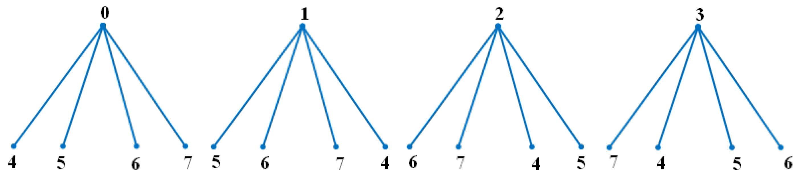
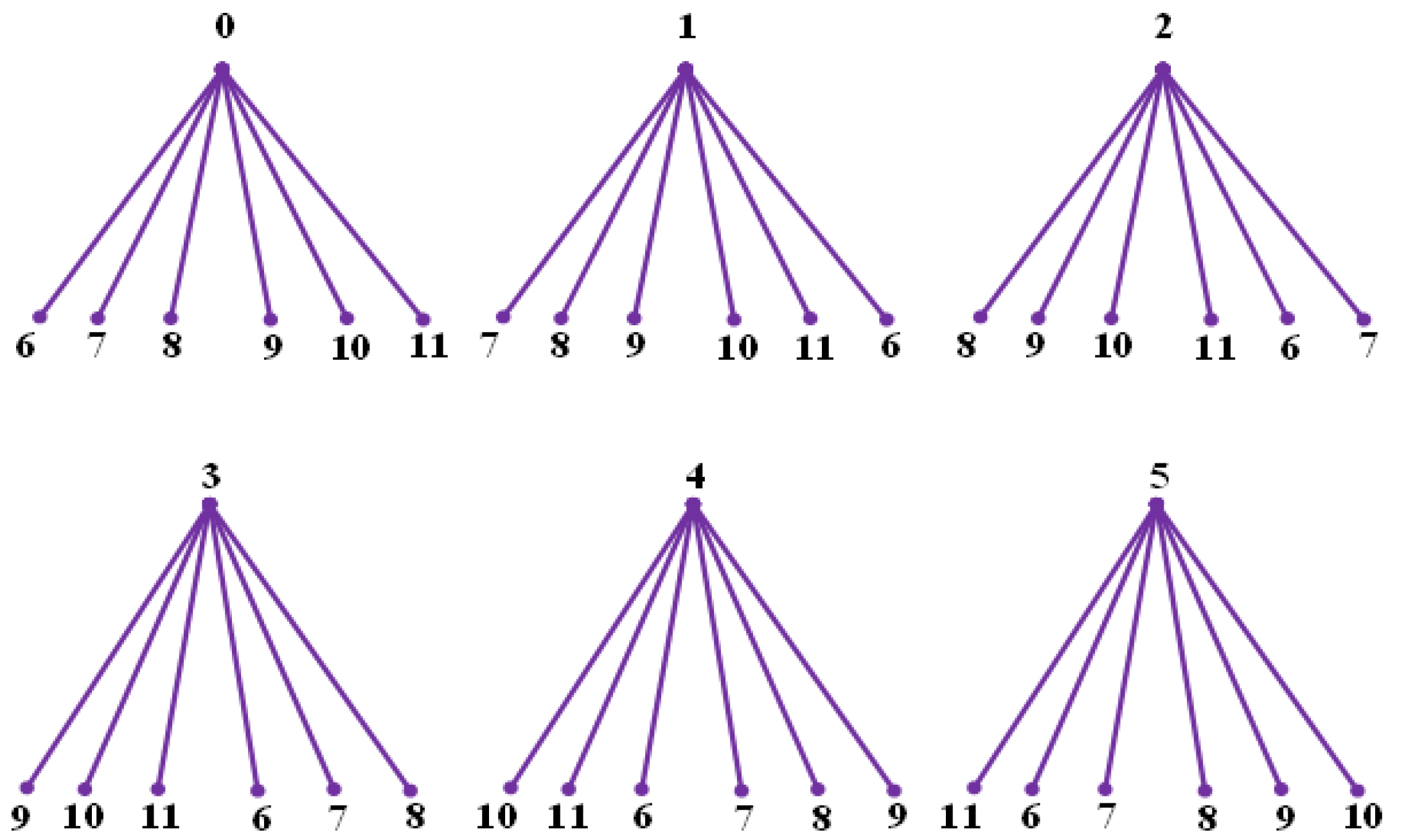
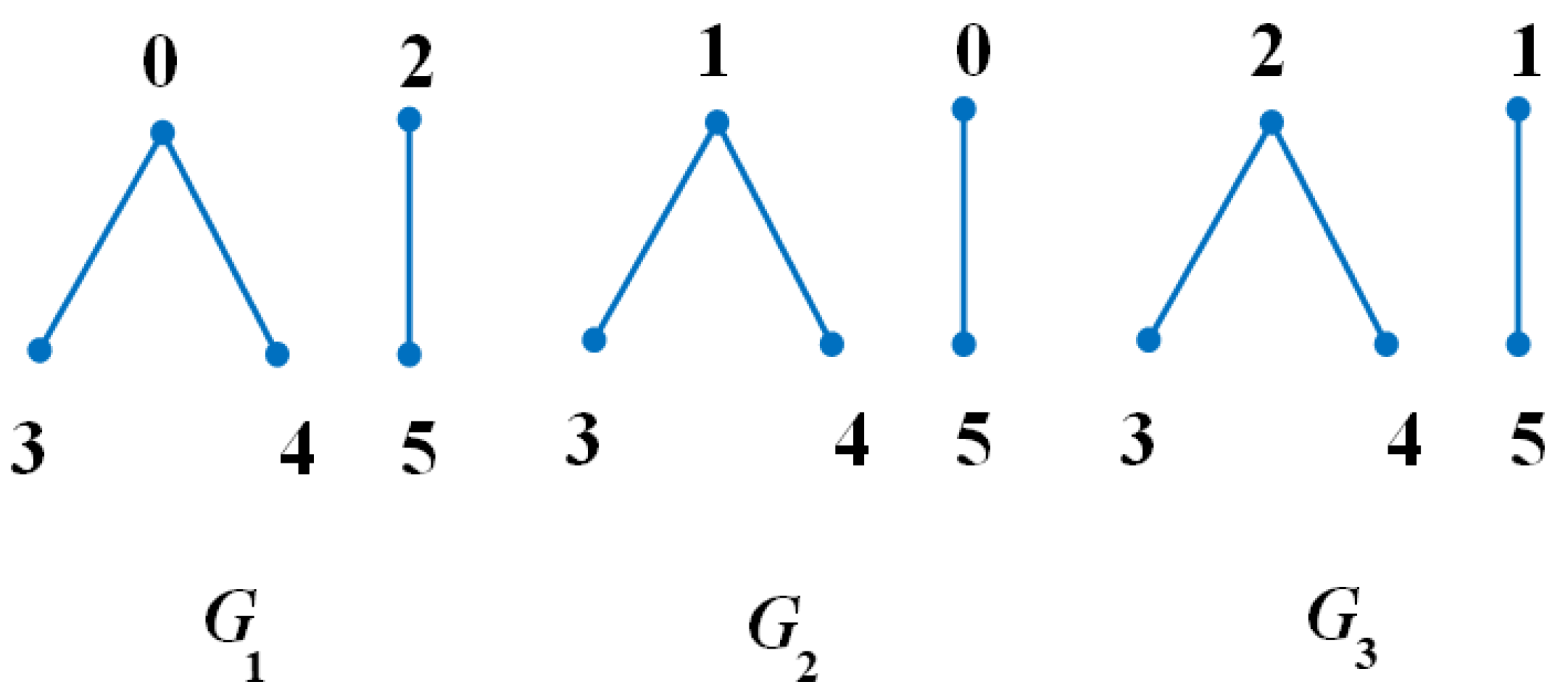
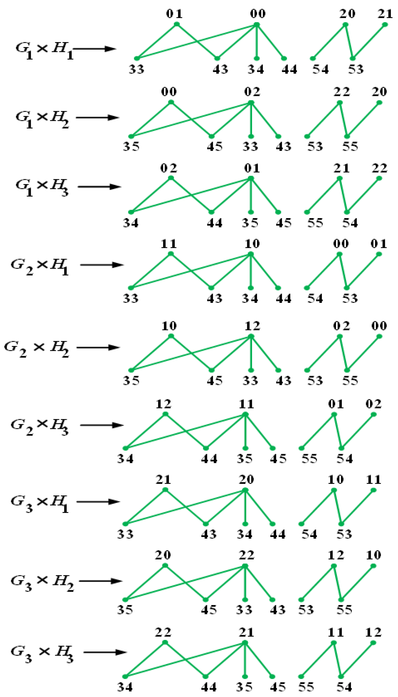
Example 1.

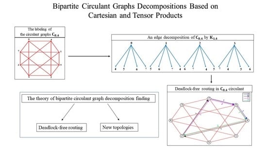
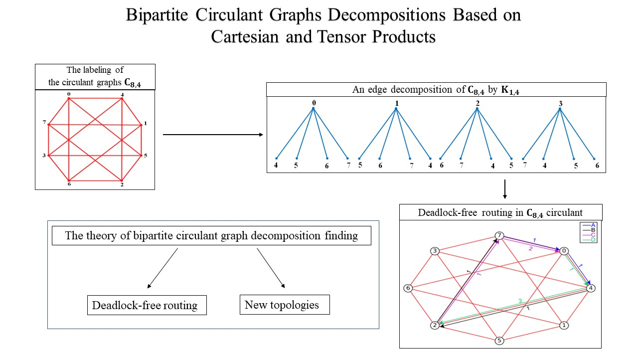
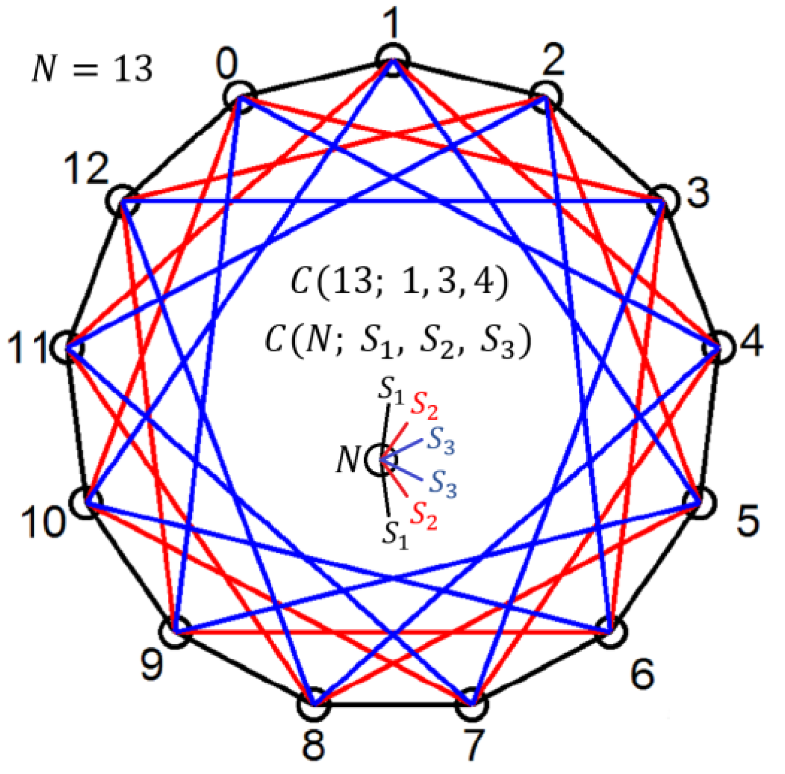
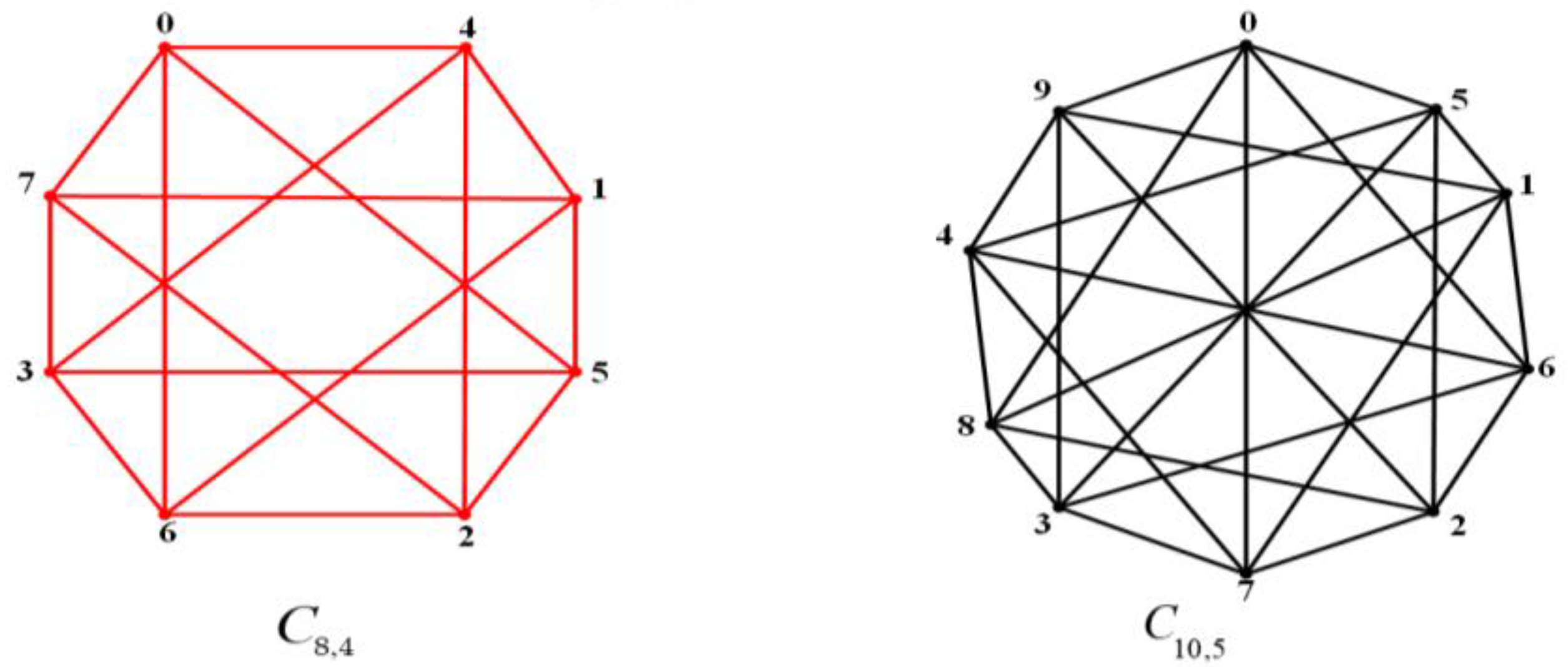
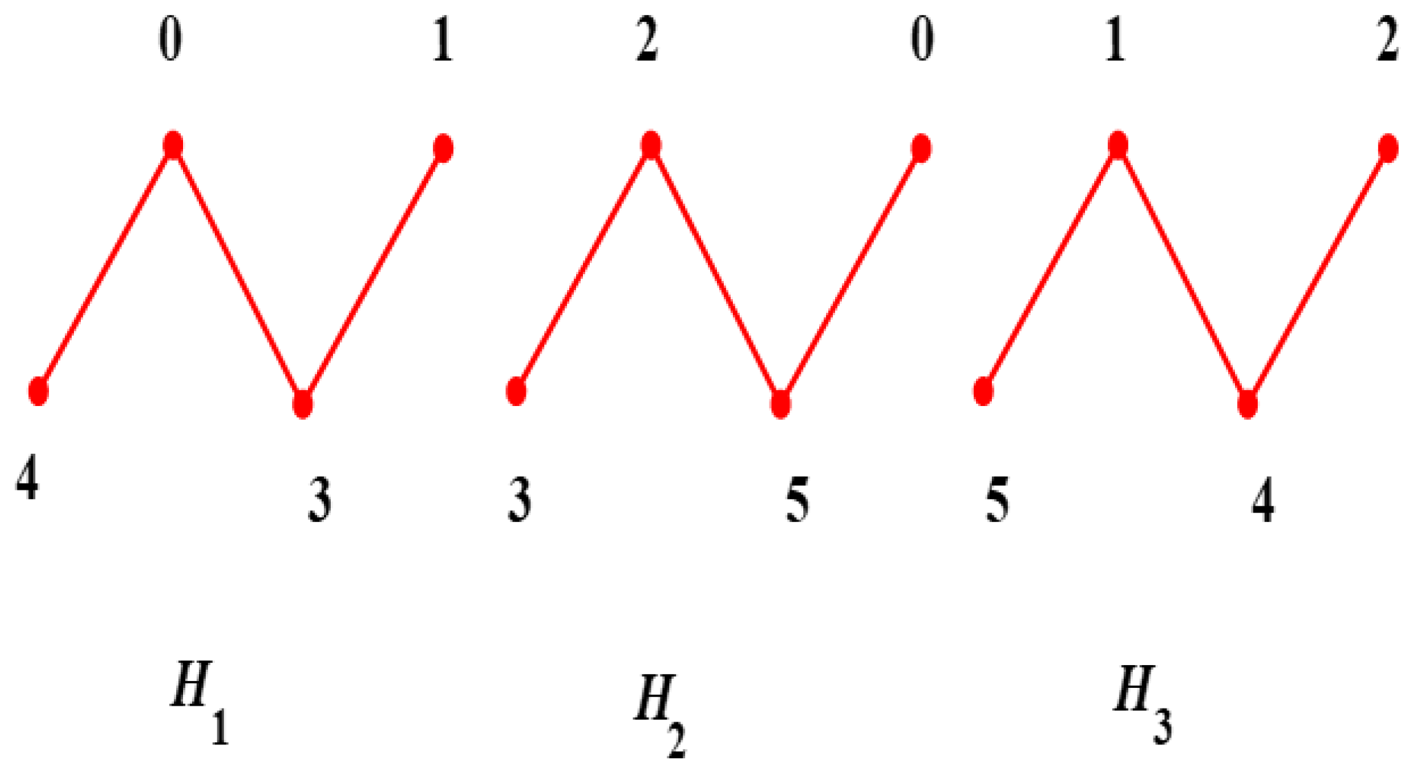
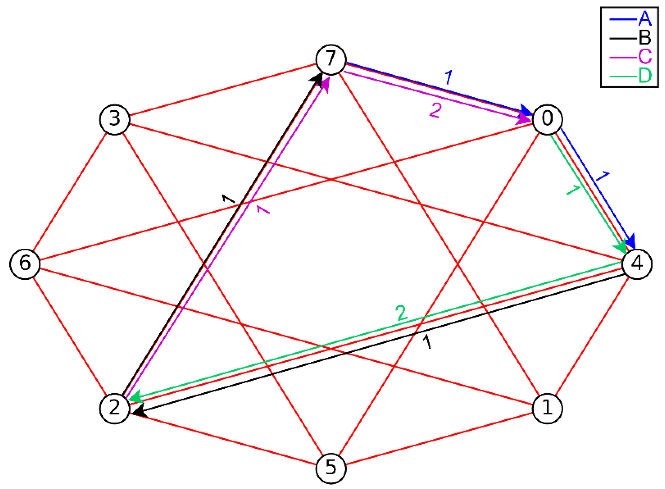
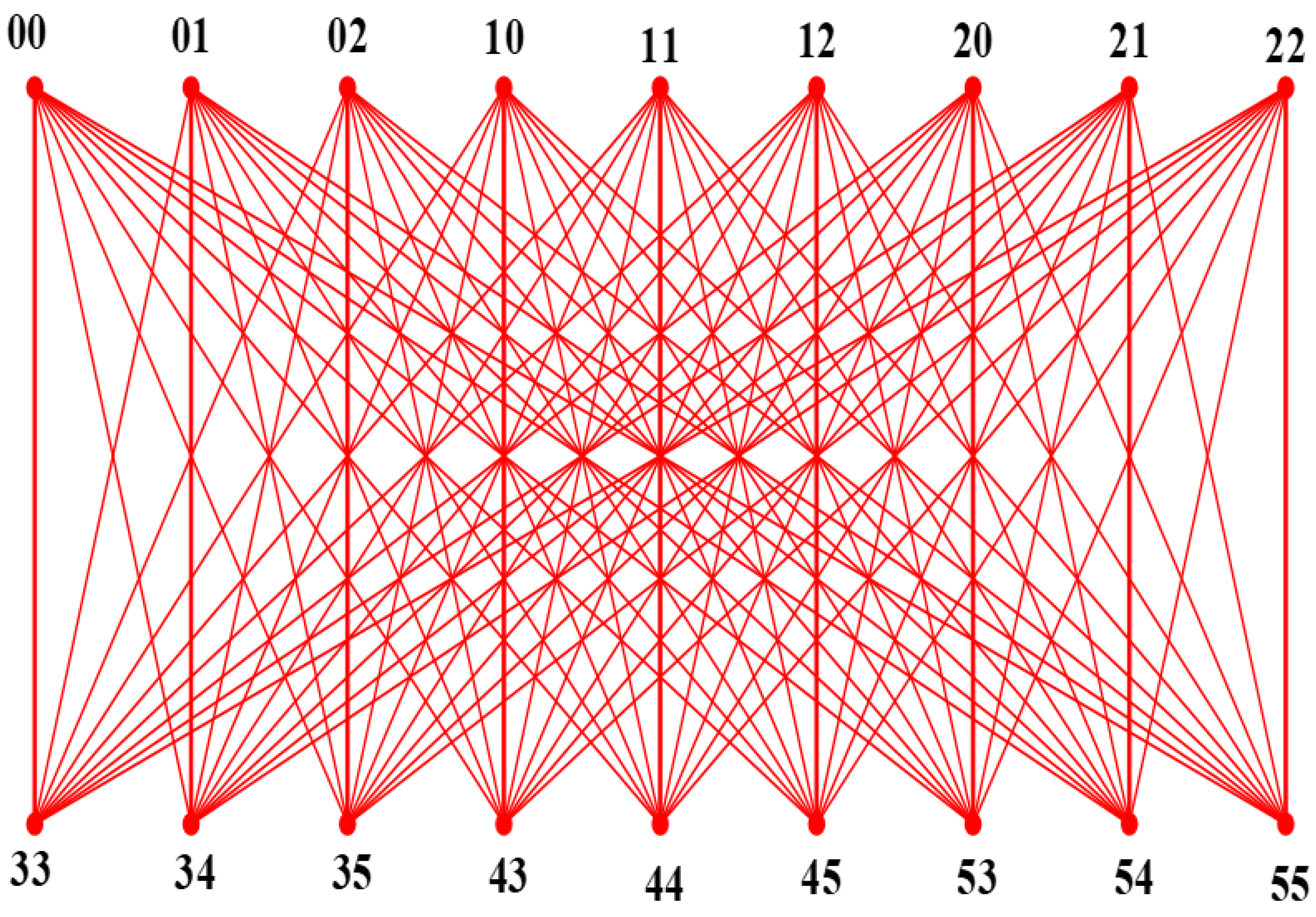
The labeling of the circulant graphs$C_{8,4}$and$C_{10,5}$is exhibited in Figure 2. Figure 3 shows an edge decomposition of$C_{8,4}$by$K_{1,4}.$In addition, an edge decomposition of$C_{12,6}$by$K_{1,6}$, based on the Cartesian product, is exhibited in Figure 4.

We provide the general tensor product method for constructing the decomposition of the circulant graphs in the section that follows.

4. Edge Decomposition of ${\mathit{C}}_{\mathsf{2}\mathsf{n}\mathsf{m},\mathsf{n}\mathsf{m}}$ Based on Tensor Products

If $A$ and $B$ are simple graphs, then the graph with the vertex set $V\left(A\right)\times V\left(B\right)$ and $E\left(A\times B\right)=\{\left(a,b\right)\left(c,d\right):ac\in E\left(A\right)$ and $bd\in E\left(B\right)\}$ is the tensor product of $A$ and $B$. The induced subgraphs $\left(A\times B\right)\left[\left(E\times Y\right){{\displaystyle \cup }}^{}\left(F\times Z\right)\right]$ and $\left(A\times B\right)\left[\left(E\times Z\right){{\displaystyle \cup }}^{}\left(F\times Y\right)\right]$ are referred to as the weak-tensor products of $A$ and $B$ if the simple graphs $A$ and $B$ are bipartite graphs with bipartitions $\left(E,F\right)$ and $\left(Y,Z\right)$, respectively. We use $A⊛B$ to represent the weak-tensor product $\left(A\times B\right)\left[\left(E\times Y\right){{\displaystyle \cup }}^{}\left(F\times Z\right)\right]$.

Proposition 2.

If there is an edge decomposition of$C_{2m,m}$by the graph$G$and an edge decomposition of$C_{2n,n}$by the graph$H,$then there is an edge decomposition of${\mathit{C}}_{\mathit{2}\mathit{n}\mathit{m},\mathit{n}\mathit{m}}$by the graph$G⊛H$.

Proof. 

Let $\mathcal{A}=\left\{G_1,G_2,\dots ,G_m\right\}$ be the edge decomposition of $C_{2m,m}$ by $G$ on $V\left(C_{2m,m}\right)=\left(E,F\right)$, where $E=\left\{e_1,\dots ,e_m\right\}$, and $F=\left\{f_1,\dots ,f_m\right\}$ is the bipartition of $C_{2m,m}$, and let $ℬ=\left\{H_1,H_2,\dots ,H_n\right\}$ be the edge decomposition of $C_{2n,n}$ by $H$ on $V\left(C_{2n,n}\right)=\left(Y,Z\right)$, where $Y=\left\{y_1,\dots ,y_n\right\}$, and $Z=\left\{z_1,\dots ,z_n\right\}$ is the bipartition of $C_{2n,n}$. Let $W=V\left(C_{2mn,mn}\right)$ and the partite sets of $C_{2mn,mn}$ be $\left\{\left(e_p,y_q\right):1\le p\le m,1\le q\le n\right\}$ and $\left\{\left(f_p,z_q\right):1\le p\le m,1\le q\le n\right\}$. Consider the set $\mathcal{C}=\left\{\left(G_p\times H_q\right)\left[W\right]:1\le p\le m,1\le q\le n\right\}$ of subgraphs of $C_{2mn,mn}$. Clearly, $\left(G_p\times H_q\right)\left[W\right]\cong G⊛H,1\le p\le m,1\le q\le n,\sin \mathrm{ce}$ $G_p\cong G\mathrm{and}$ $H_q\cong H$. □

Claim 1.

Every edge of $C_{2mn,mn}$ occurs in exactly one graph of $\mathcal{C}.$

Consider an arbitrary edge $\left(e_s,y_t\right)\left(f_u,z_v\right)$ of $C_{2mn,mn}.$ Since $\mathcal{A}$ is an edge decomposition of $C_{2m,m}$ by $G$, and $ℬ$ is an edge decomposition of $C_{2n,n}$ by $H,$ the edges $e_s{f}_u$ and $y_t{z}_v$ are, respectively, in exactly one graph of $\mathcal{A}$ and $ℬ.$ Let the graph containing $e_s{f}_u$ be $G_{t_1}$, and that of $y_t{z}_v$ be $H_{r_1}.$ Then, the graph containing the edge $\left(e_s,y_t\right)\left(f_u,z_v\right)$ is $\left(G_{t_1}\times H_{r_1}\right)\left[W\right]$.

Claim 2.

Any two graphs in $\mathcal{C}$ have no edges in common.

The two graphs $\left(G_{t_1}\times H_{r_1}\right)\left[W\right]$ and $\left(G_{t_2}\times H_{r_2}\right)\left[W\right]$ have no edges in common, because $|E\left(G_{t_1}\right){{\displaystyle \cap }}^{}$ $E\left(G_{t_2}\right)|=0$ and $|E\left(H_{r_1}\right){{\displaystyle \cap }}^{}$ $E\left(H_{r_2}\right)|=0$.

Example 2.

Figure 5 shows an edge decomposition of$C_{6,3}$by$K_{1,2}{{\displaystyle \cup }}^{}{K}_2.$Figure 6 shows an edge decomposition of$C_{6,3}$by$P_4.$In addition, an edge decomposition of$C_{18,9}$by$\left(K_{1,2}{{\displaystyle \cup }}^{}{K}_2\right)⊛P_4$is exhibited in Figure 7.

5. Use Case

5.1. Routing Problem in Bipartite Circulant Graphs

As shown earlier, circulant graphs have a wide range of applications. They are especially promising for communication networks for supercomputer systems and NoCs. The fact is that in wired communication networks, the classic are various tree-like topologies [42] (formally, combination of bus and star network topologies). This is due to the hierarchical structure of such networks, where routers of different levels are connected, and end devices are leaves of such a tree. Such topologies are also convenient in that they can contain a predetermined number of nodes that can dynamically connect and disconnect. However, at the same time, trees also have many disadvantages, such as a long path between nodes, the congestion of connections located closer to the root nodes, etc.

In closed networks (such as communication subsystem of a supercomputer), the topology and the number of nodes are usually predetermined. Therefore, they normally use much more efficient, more connected topologies, such as mesh and torus [43]. They are convenient in that they have a flat shape and a regular structure, so that network nodes can be easily networked. At the same time, routers are also quite simple, and they are of the same type.

It can be noted that NoCs are (to some extent) analogous to supercomputer networks; the only difference is the processing nodes are placed inside one chip; there is also the problem of finding new regular topologies to connect nodes.

With the development of technology, topological characteristics (such as diameter and mean path length) are becoming even more important; mesh and torus are most effective when they are square-shaped, i.e., this way, they limit the set of nodes that the network can consist of. It is known [44] that circulant topologies have better topological characteristics and also endure any number of nodes, i.e., they are a promising replacement for the classical regular topologies.

An important requirement for routers in the networks considered is their simplicity; so, there is no need to implement the whole OSI [42,45] networking model and multi-layer communication protocols. Ideally, the router should contain a finite-state machine that, based on the known destination address and its own address, calculates which port to forward the packet to. On the other hand, such simplicity leads to the fact that the communication subsystem becomes vulnerable to various destructive phenomena, such as deadlocks, livelocks, failures, and starvation [46,47]. Deadlocks occur due to the presence of cyclic dependencies in packet transmission routes, when the tail of one packet blocks the head of another packet, whose tail (in turn) blocks another packet, and so on.

For mesh and torus, many different methods of dealing with deadlocks have been developed, many of which are based on the use of virtual channels and sets of rules for switching between channels and bypassing blocked links [46]. However, for circulant topologies, there are few such approaches, since it is not entirely clear which rule should be used to switch virtual channels.

To handle deadlocks, we propose to divide the graph using edge decomposition into a set of simpler subgraphs that do not have cyclic dependencies (see Figure 2 and Figure 3). The following rule can be introduced: if a packet moves from one subgraph to another, it has to change the virtual channel. At the same time, at the beginning of moving through the network, a packet is always in virtual channel 1.

This approach is primarily applicable for local distributed routing, when the entire path is not calculated in advance, and the decision to switch the packet to the appropriate port is made at the router level and only 1 hop ahead. Thus, adding an additional virtual channel selection rule will lead to a slightly more complicated routing procedure and the need to store 1–2 additional bits denoting the subgraph label to which the corresponding router belongs. Against the background of the total resource consumption of the router, according to the experience of previous studies [48], such a complication should not affect the resource consumption of the router. This statement needs to be verified in the future.

Example 3.

Consider how proposed rule works based on the example of graph$C_{8,4}$.

Suppose there is a situation of a cycle of vertices $0->4->2->7->0$, and according to the rules of the routing algorithm (it is static, not adaptive [46]), the packets move clockwise along this cycle. We need to transfer the data from node 7 to node 4 (packet A), from 4 to 2 (packet B), from 2 to 0 (packet C), and from 0 to 2 (packet D). As a result, a deadlock situation arises, because packet A will block packet C, which (in turn) will block packet B, and through it packet D, which interferes with A. Using the proposed rule, the deadlock will be eliminated, since packets C and D (on the second hop) will cross the boundaries of the subgraph (Figure 8) and switch to virtual channel 2 with no path blocking.

A few more simple rules to help resolve deadlocks can be proposed. The most important is the fact that the proposed plane tessellation methods allow you to mark up a graph into a set of simple subgraphs without cycles, based on which it is possible to build deadlock-free routing algorithms.

5.2. New Bipartite Circulant Topology Generation Using Cartesian and Tensor Products

The problem of searching for new topologies for NoCs and supercomputers can also be taken another look at: while supercomputers are already capable of containing tens of thousands of computing nodes [49], chips have recently also reached such sizes that they can accommodate a huge number of computing cores [50,51]. At the same time, finding the optimal circulants for hundreds of nodes is already a rather difficult task [49]. There is a significant number of works that offer various methods for generating new topologies. These are both hierarchical topologies [52,53,54] and topologies obtained by the graph product [55] (a special case is optimal circulant product [52]), etc. However, as shown earlier, it is not enough to propose a new topology and evaluate its characteristics. We still need to develop the effective routing algorithms, as well as methods for dealing with deadlocks. Therefore, we propose to consider this problem from the reverse: one can choose a basic subgraph without cycles and then, based on it, use the methods of Cartesian and tensor products to generate new topologies. Thus, in such graphs, it can be guaranteed that the method of dealing with deadlocks, described in Section 5.1, can be applied.

Example 4.

According to Figure 3, the bipartite circulant graph $C_{8,4}$can be generated from the graph $K_{1,4}$.

Example 5.

Based on tensor product in Example 2 in Section 4, the union of the graphs in Figure 7 provides $C_{18,9}$shown in Figure 9.

6. Conclusions

In conclusion, we introduced the Cartesian and tensor product approaches as supporting tools for the decompositions of bipartite circulant graphs into many categories of graphs. The use cases of applying the described theory of bipartite circulant graph decomposition to the problems of finding new topologies and deadlock-free routing in them when building supercomputers and NoCs are considered.