Abstract
It is known that the protein surrounding, as well as solvent molecules, has a significant influence on optical spectra of organic pigments by modulating the transition energies of their electronic states. These effects manifest themselves by a broadening of the spectral lines. Most semiclassical theories assume that the resulting lineshape of an electronic transition is a combination of homogeneous and inhomogeneous broadening contributions. In the case of the systems of interacting pigments such as photosynthetic pigment–protein complexes, the inhomogeneous broadening can be incorporated in addition to the homogeneous part by applying the Monte Carlo method (MCM), which implements the averaging over static disorder of the transition energies. In this study, taking the reaction center of photosystem II (PSIIRC) as an example of a quantum optical system, we showed that differential evolution (DE), a heuristic optimization algorithm, used to fit the experimentally measured data, produces results that are sensitive to the settings of MCM. Applying the exciton theory to simulate the PSIIRC linear optical response, the number of minimum required MCM realizations for the efficient performance of DE was estimated. Finally, the real linear spectroscopy data of PSIIRC were fitted using DE considering the necessary modifications to the implementation of the optical response modeling procedures.
1. Introduction
The Monte Carlo method (MCM) is one of the most common computational algorithms based on the use of randomly distributed parameters with which it is possible to obtain the numerical solutions to a problem that, in general, can be either probabilistic or deterministic in nature [1]. This method has already been tested and implemented in different areas of experimental and applied sciences, such as physics [2], mathematics [3], engineering [4,5], biology [6,7], medicine [8] and others [1]. In physics- and mathematics-related problems, MCM is very useful if there is no way to obtain an exact analytical solution, particularly in the modeling of the optical response of photosynthetic pigment–protein complexes (PPC), when the inhomogeneous broadening of Qy electronic transition of chlorophylls (Chls) and bacteriochlorophylls has to be taken into account [9,10].
Experimental and theoretical research on the optical properties of PPCs is an essential part of the study of photosynthesis as a fundamental process in nature [11]. PPCs are functional subunit proteins of the photosynthetic apparatus of higher plants and bacteria located in cell membranes [12]. Most of them serve as light-harvesting complexes that absorb light quanta, which are subsequently converted into excited states of the complexes [13,14]. Excited states migrate along PPC until they are localized in the special complexes’ reaction centers, where the charge separation takes place [15]. Generally speaking, all PPCs consist of pigment molecules bound to the protein matrix. Remarkably, the pigments are tightly fixed in their positions, forming a rigid spatial structure. The spatial structure of the pigments determines the coupling energies between excited states of molecules, thereby having a significant influence on the optical properties of PPC [16,17]. Thus, in order to simulate the optical response of PPC most accurately, it is necessary to use a theory that will simultaneously account for both the spatial arrangement of the pigments, and the effect of the protein environment and electron–phonon interaction [18].
MCM has been used quite often to model the results of spectroscopy measurements made on PPC samples [17,19,20]. In this case, MCM allows taking into account the effect of slow modulations of an electronic transition which is caused by interactions with the corresponding nuclear degrees of freedom [10,21,22]. To do so, the diagonal elements of the Frenkel exciton Hamiltonian are modified by a Gaussian fluctuation parameter and the resulting spectrum is calculated by the averaging of this parameter over all realizations [23,24,25]. It is clear that the amount of computational work required for modeling the optical properties of PPC strongly depends on the number of pigments in PPC whose excited states are considered. For example, photosystem I monomeric and trimeric complexes contain about 100 and 300 pigments, and modeling the linear spectroscopy for such complexes is already a time-consuming exercise [17]. This is why we decided to employ the reaction center of photosystem II (PSIIRC) as a model for PPC. Firstly, it contains only eight porphyrin-like pigments (6 Chls and 2 pheophytins); secondly, there are many available experimental data measured at different temperatures, as well as theoretical studies on energy transfer and charge separation in PSIIRC.
Application of any optimization algorithm for the fitting of PPC experimental data is a non-trivial task, since the exciton theory and the multimode Brownian oscillator model used for the spectra simulation have many input parameters and, most importantly, the dependence of simulated spectra on some parameters is nonlinear [9,12,21]. The use of evolutionary strategies as an optimization scheme, particularly a metaheuristic search procedure such as the genetic algorithm, can be considered successful for this kind of problem [26]. The first attempts at modeling kinetics and the exciton dynamics in photosystem I [27], simulating the spectroscopic characteristics for the light-harvesting complex II from higher plants [28], localization of the triplet states in PSIIRC [19], linear spectroscopy of monomeric photosystem I [17] and a study of red chlorophylls in photosystem I [29] have been made in the last 25 years applying the genetic algorithm. Nevertheless, the differential evolution algorithm (DE) [30,31] can be considered a more appropriate method for modeling primary photosynthetic processes. Compared with other evolution algorithms, DE deals with the real type variables allowing the fitting parameters to be varied continuously during program run [32,33].
Recent reviews on applications of DE have shown [32,34] that, in addition to the classical version of the algorithm, so-called self-adaptive DE modifications [35,36,37,38], designed to improve convergence, are now actively used for many tasks [39]. However, these modifications in the case of PPC optical properties modeling have no significant effect on the convergence rate and the spectra fitting results. To deal with this situation, we have developed software combining the DE algorithm and procedures for the calculation of the spectra of photosynthetic pigments and pigment–protein complexes [40,41]. Starting with the modeling of linear absorption of monomeric Chl, bacteriochlorophyll and carotenoids in different solvents, the best DE strategy and its optimal settings have been found [41,42]. The next step was to explore the prospect of using DE to fit the linear spectroscopy of a small PPC, such as PSIIRC. Having a set of artificially simulated spectra as experimental data, we were able to match the DE settings with which the algorithm found the required parameters of the exciton model of PSIIRC [40]. However, it makes no sense to use such a model to fit experimentally measured spectra, since it does not take into account the inhomogeneous broadening of the PSIIRC excited states (Figure 1).
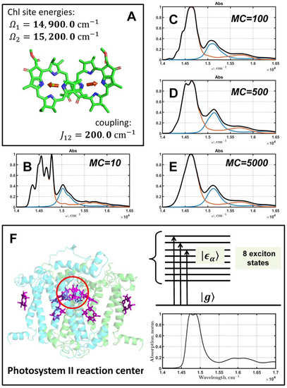
Figure 1.
Effect of the inhomogeneous broadening on the optical properties of PPC. A dimer of coupling Chls (A) with Qy transition moments (red arrows) is shown with parameters of the exciton Hamiltonian (5). Calculated absorption spectra of the dimer are presented for different MC values: 10 (B), 100 (C), 500 (D), 5000 (E); FWHMΩ = 300 cm−1. The black line is the resulting dimer absorption, and the red and blue lines are absorptions of the excited states of a dimer. Parameters of the spectral density of the Qy transition of Chl was taken from [40]. The crystal structure of PSIIRC: positions of Chls and pheophytins and protein subunits. The red circle marks D1–D2 special pair—two Chls where charge separation processes take place. Coupling cofactors of PSIIRC creates an exciton manifold of eight states with the characteristic absorption at 77 K (F).
Thus, the aim of this study is to enhance the previously published PSIIRC exciton model and the quality of linear optical properties modeling [40] by adding the procedure of inhomogeneous broadening by means of MCM. It must be stressed that MCM is a probabilistic method which provides only an approximate solution to a problem. On the other hand, DE is also based on a random generator in order to create new populations of parameters. Therefore, the question arises whether the two probabilistic methods can be used in the same harness, and whether the convergence of DE will be affected by using MCM to simulate the optical response of PPC? Moreover, is it possible to fit measured experimental data with such a combination of methods, while simultaneously obtaining significant parameters for quantum models of primary photosynthetic processes? Thus, our study focuses on answering these two questions.
2. Theory of the Optical Response with Inhomogeneous Broadening
A detailed description of the quantum model of PSIIRC without taking into account of the inhomogeneous broadening has been given in our previous published paper [40]. Considering the multimode Brownian oscillator model to calculate the spectral density and the lineshape function for cofactors of PSIIRC, and the exciton theory to simulate the optical response of a system of coupling pigments [9], the final expressions in terms of the modified Redfield theory [43,44] for absorption , linear , circular dichroism and steady-state fluorescence of PSIIRC were written as follows:
where and are the eigenvalues of the Frenkel Hamiltonian of PSIIRC and the corresponding squares of the Qy transition moments of Chls and their components, is the lineshape function in the exciton representation, is the relaxation rates of the exciton states, is the reorganization energy, which represents the influence of vibronic modes on the exciton state, enumerates the exciton states, N is the number of pigments in PSIIRC [40], , is the rotation strength matrix of PSIIRC needed to estimate the effect of circular dichroism, are the eigenvectors and are distances between Chls. It is worth adding that PSIIRC consists of two types of pigments optically active at 600–700 nm: Chls and pheophytins. In fact, they have to be characterized by two different spectral densities; however, we used the same spectral density for all pigments in our simulations. Generally, this simplification will not affect the results of the test of MCM and DE working together, but to analyze the energy transfer and charge separation in PSIIRC in detail, two spectral densities have to be considered.
To incorporate the inhomogeneous broadening employing MCM, the diagonal elements of the Frenkel Hamiltonian PSIIRC must be modified by a fluctuation parameter:
where is a set of fluctuations generated by a Gaussian random number generator. The output of the generator is controlled by the full width at half maximum , is the index of MCM realizations and MC is the maximum number of MCM realizations.
The interaction energies between transition moments of the pigments were estimated in the dipole–dipole approximation:
where is the dielectric constant, an effective parameter, which is used for the spectra fitting to tune energies and is the dielectric permittivity of classical vacuum. The dipole–dipole approximation works nicely when . This condition is satisfied for all cofactors in PSIIRC except the D1–D2 special pair (Figure 1). can be calculated by another method such as the extended dipole–dipole approximation [45], however, for the purposes of our study we will use the results of other studies [23,46,47], and consider in the modeling.
Thus, is diagonalized for each step of MCM, the calculated spectra (1–4) are saved every time and finally, when MCM cycle is finished, the resulting spectra are averaged over all realizations.
where denotes the MCM average over MC realizations.
3. Differential Evolution
To fit the PSIIRC linear spectroscopy data, the classical version of DE was used [31]. The developed software, together with the spectra simulation procedures, contains the implementation of four steps of DE data processing: (1) initialization of the parameter population, (2) creating the mutation vectors, (3) crossover and (4) parameters selection for the new generation [40,41]. Previously, DE has been successfully applied to fit the linear optical response of monomeric Chls, bacteriochlorophylls and carotenoids in different solvents. As the result, two strategies, DE/rand-to-best/1/exp and DE/best/1/bin, have shown high performance and convergence rates. The tests of DE with artificially created experimental data of PSIIRC without inhomogeneous broadening revealed the same effectiveness for these two strategies. Being tested for the ranges of the weighting factor and the crossover probability , it was found that DE/rand-to-best/1/exp with and [40] are the optimal parameters to fit PSIIRC data. We used the same settings of DE to conduct the fitting with inhomogeneous broadening.
The cost value of a mutant vector for a current generation of DE is estimated as follows:
where spec is the index of PSIIRC spectra: , are the arrays of either artificially created or measured experimental data and are the simulated spectra by evaluating Equations (7)–(10).
4. Results
4.1. Inhomogeneous Broadening of a Chl Dimer
To demonstrate the effect of inhomogeneous broadening on a system of coupling pigments, let us consider a dimer of two Chls spaced within about 10Å (Figure 1A). Chls have two pronounced absorption bands in the visible range: the high-energy Soret band (Bx, By electronic transitions) at 350–450 nm, and the Qy transition at 600–700 nm. We will focus on the optical response of the Qy transition, thus, to construct the eigenstates and the eigenvalues of the dimer, the 2 × 2 Hamiltonian (5) will be used with , and . The lineshape function of a monomeric Chl is calculated at 77 K, applying the spectral density taken from [40]. The effective length of the Qy transition dipole moment is 0.9 Å. The time and frequency scales consist of points.
The importance of correct averaging when using MCM is shown by producing a series of inhomogeneously broadened dimer spectra; was taken to be to generate fluctuations for diagonal elements of the Hamiltonian in Equation (5). The simulated spectra are depicted in Figure 1B–E for four values of MC: 10, 100, 500, and 5000.
4.2. PSIIRC Linear Optics Simulations with Different MC
The example of dimer absorption modeling clearly shows how important it is to understand from what value of MC the obtained spectra can be considered sufficiently averaged. Naturally, the extreme high MC provides proper averaging; however, it is always better to know the moment when we can stop MCM without loss of accuracy to save computational time.
Before starting the fitting of the measured experimental data, preliminary simulations of PSIIRC optical properties were made in order to estimate MC. We used the parameters of Table A1 from [40] to create the 8 × 8 exciton Hamiltonian, Qy electron transition energies for each PSIIRC cofactor and interaction energies in the dipole–dipole approximation. The absorption profile of monomeric pigments was calculated in the same way as for the Chl dimer. We used the following set of MC to evaluate Equations (7)–(10): 100, 200, 500, 1000, 2000, 5000 and 10,000. Fluctuations of the diagonal elements of the Hamiltonian were estimated for . For each MC, linear spectra were simulated seven times and the differences between absorption spectra were calculated according to formula: , where , are the indexes enumerating PSIIRC spectra for each MC. The results of the simulation are listed in Table A1. Graphic visualization of as well as histograms of fluctuation parameter distribution for the first pigment in PSIIRC are represented in Figure 2. The differences between spectra calculated at MC = 10,000 and the other six values of MC are shown in Figure 3.
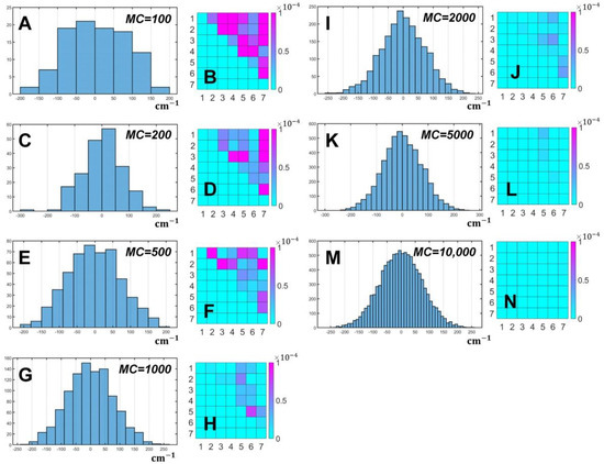
Figure 2.
Distribution of the fluctuation parameter for the first transition energy in the Hamiltonian (5) for the following MC values: 100 (A), 200 (C), 500 (E), 1000 (G), 2000 (I), 5000 (K), 10,000 (M). For each MC, absorption spectrum of PSIIRC was simulated seven times, and then the spectra were compared with each other by calculating for each pair of 21 combinations of the spectra. The resulting matrices of are shown for MC = 100 (B), 200 (D), 500 (F), 1000 (H), 2000 (J), 5000 (L), 10,000 (N). Color bars reflect the variations of .
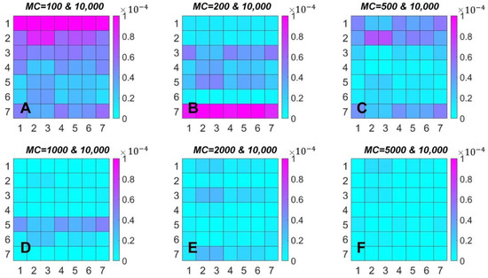
Figure 3.
The same data as in Figure 2. Demonstration of the differences between spectra calculated at MC = 10,000 and the other six values of MC. X-axis of each matrix corresponds to seven spectra with MC = 10,000, Y-axis enumerates spectra for MC = 100 (A), 200 (B), 500 (C), 1000 (D), 2000 (E), and 5000 (F). Color bars reflect the variations of .
.
4.3. Tests of DE with the Artificial Experimental Data
Considering the results described in the previous section, we can conclude that MCM with MC = 10,000 gives the “smoothest” spectra. However, such a number of MCM realizations is unacceptable for DE optimization, since the amount of trial function calls is in the thousands and to complete the fitting in a reasonable time, MC has to be reduced. To carry out a simple test of the DE dependence on MCM, we set PSIIRC spectra simulated at MC = 10,000 as the target functions for absorption, fluorescence, circular and linear dichroism. To test the convergence of DE, optimization was run for one and two free parameters of PSIIRC quantum model; all the other model parameters were fixed. In both cases (one and two free parameters) DE was run five times for the following values of MC: 100, 200, 500, 1000, and 2000. The results of the tests are collected in Table A2 and Table A3.
4.4. Tests of DE with the Real Experimental Data
Based on the DE tests with artificial experimental data, MC = 500 was chosen to run the fitting of real experimental data. PSIIRC linear spectroscopy was taken from two sources: absorption and steady-state fluorescence spectra are from [48] and dichroism spectra are from [25]. The total number of free parameters of the PSIIRC exciton model was eleven: eight electron transition energies , the dielectric constant ε to scale the Chl-Chl coupling energies (6), the full width at half maximum of inhomogeneous broadening , and the D1–D2 special pair coupling . Some features of the applied PSIIRC exciton model and DE settings can be found in [40]. DE was run ten times; the best results are presented in Figure 4.
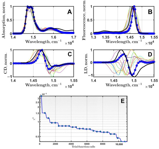
Figure 4.
Fitting of the PSIIRC linear optical spectroscopy measured at 77 K. Black thick lines are the experimental spectra. The best results of optimization (blue lines with circular markers) for absorption (A), steady-state fluorescence (B), circular (C), and linear (D) dichroism are presented. Thin, colored lines are the simulated spectra found by DE after the first 10 generations. evolution during 100 generation of DE (E).
5. Discussion
By analyzing and comparing the quantum models of the simple Chl dimer and rather more complex proteins such as PSIIRC, it becomes clear that the required number of MCM realizations depends precisely on the relation between the parameters of the exciton model. The dimer of Chls, used as an example, has , ; the corresponding eigenvalues are 14,800 cm−1 and 15,300 cm−1. Such eigenvalues give a gap of 500 cm−1 which is greater than . As a result, absorption bands of the dimer are well separated in the spectrum (Figure 1B–E). This means that if we want to achieve a smooth quality spectrum, it is necessary to set a large value for MC. For a simple model such as a dimer, there is no problem with running optimization with thousands of MCM realizations, but for a system of many pigments, especially with sparse absorption bands, this may already be problematic.
Potential exciton models of PSIIRC have already been discussed many times [19,23,46,47,49]. Characteristic features of PSIIRC include small differences between transition energies of cofactors , coupling energies and . This exciton configuration leads to an optical response in which the exciton states are either close together, or overlap with each other. The resulting spectra look relatively broad and featureless, however, at lower temperatures some peculiarities do emerge (Figure 1F). It is obvious that fitting experimental data with such models is hardly possible without optimization, however, much of the analysis has been carried out by hand.
DE seems to be a promising solution to fit experimental data of PPC. Studies of the optical properties of monomeric photosynthetic pigments in different solvents with DE have proved to be quite optimistic [41,42]. To proceed with PSIIRC modeling considering MCM for inhomogeneous broadening, the effect of MC on the averaged spectra has to be investigated. Generally, with increasing MC, the perfection of simulated data increases; the higher MC value, the better. However, any experimental data have their limits of perfection, which are determined by errors of measurements and other physical effects that are not included in the mathematical description of the model. Therefore, it is clear that, to analyze the experimental data, there must be an optimal value of MC which will speed up MCM and, on the other hand, will provide enough perfection for the simulated spectra to match the quality of the measured ones.
The simulation of PSIIRC spectra was carried out for MC equal to 100, 200, 500, 1000, 2000, 5000 and 10,000. To estimate the difference in the optical response, without loss of generality, only absorption spectra were used. The results are shown in Figure 2. Plots A, C, E, G, I, K and M of Figure 2 present an example of the statistical distribution of for ChlD1 of the special pair. Histograms for 2000, 5000 and 10,000 MCM realizations demonstrate symmetrical Gaussian profiles, while distributions with smaller MCs have asymmetry and exhibit a clear lack of sampling. The differences between spectra with the same MC stored in the matrix are shown in plots B, D, F, H, J, L and N of the same figure. Table A1 contains for all MC and also the median and worst differences. One can observe an unambiguous dependence: with an increase in realizations, their median and worst values decrease.
For 10,000 realizations, the worst does not exceed -6 orders of magnitude, which suggests that this amount of MC will be enough. At the same time, when MC = 5000, although there are predominantly -6 orders of magnitude, this does not give an exact guarantee of the required simulation results.
It is interesting to compare the spectra simulated with different MC. Using spectra with MC = 10,000 as a reference, we calculated the differences according to . The results are shown in Figure 3. If MC = 1000, 2000 and 5000, the order of is about -5 and we can consider these PSIIRC spectra to be very close to those simulated at MC = 10,000, while MC = 100 and 200 give large differences between spectra.
Before the fitting of measured data, we conducted preliminary DE runs with spectra calculated at MC = 10,000 as target functions. To obtain a definitive answer to the question of which value of MC is preferable when calculating the optical response, we ran two datasets with one and two free parameters. Moreover, is a fixed parameter in the first dataset and free in the second one. The results for one free parameter are in Table A2; decreases with an increasing number of MCM realizations and reaches -6 orders of magnitude at all five runs at MC = 500. Similar values for were obtained for modeling with two free parameters (Table A3). gradually tends from 175 (MC = 100) to 182 (MC = 2000), which is closer to 180. The standard deviation of also decreases rapidly as MC realizations increase. At the same time, it is difficult to say about the unambiguous dependence of the standard deviation of dielectric constant on MC for both cases. This can be explained by the fact that its standard deviation is initially small, and these meanings of the standard deviations are a consequence of stochastic processes. Therefore, balancing between reasonable computational time and the quality of simulated spectra, we decided to take MC = 500 as optimum to fit the real data.
The best results of the fitting of PSIIRC linear spectroscopy data after ten runs of DE are presented in Figure 4. Eleven free parameters of the exciton model were considered for simulation. The overall quality of the fit can be regarded as satisfactory; however, circular and linear dichroism definitely require additional improvement (Figure 4C,D). First of all, it should be stressed that to achieve better fitting, at least another three free parameters must be added to the current set of eleven. These are the frequency, the Huang–Rhys factor and the damping factor, of the lowest frequency mode used to calculate the spectral density of a pigment [40,41,42]. At the moment, there are some technical problems preventing such improvement of our software and considering these three parameters in the fitting, but this is our immediate goal to enhance computational procedures.
decreased quite fast in the first ten generations, and then there was a slow asymptotic stagnation. Similar behavior of was observed in the modeling of monomeric pigments’ absorption in solvents [41,42]. The maximum number of generations was set to 100. This definitely has to be increased up to 300 or 400 [40], but for the first attempt at running the fitting, it was decided to use 100.
Interestingly enough, the , the coupling between special pair Chls, can be estimated without any optimization simply using physical theories describing the interaction of electronic excited states [45]. Aside from the magnitude of , the sign is also important (positive–repulsion, negative–attraction). Calculations for the D1–D2 dimer give the positive sign. On the other hand, was a free parameter in the fitting with initial boundaries . As a result, the best convergence was exclusively achieved for the positive values of . Thus, we can state that DE optimization is sensitive to the exciton model of PSIIRC.
To summarize the work carried out, the combined use of MCM and DE optimization is feasible and the first runs of PPC fitting optical spectroscopy have been successful. It is clear that the software needs further improvements as well as additional research related to its performance. In the future, the main upgrade of the computational procedures will be to add the routines for simulation of PPC nonlinear optical experiments.
6. Conclusions
Unravelling the mechanisms of the primary physical processes in PPC is directly related to the creation of quantum models and the fitting of spectroscopic data. The structure of PPCs and arrangement of pigments in PPCs are such that the application of rigorous analytical solutions to simulate the optical response is not possible. Thus, using the semiclassical theories together with optimization algorithms is an ideal solution for this kind of problem. We have developed special software that allows the linear optical response, namely absorption, steady-state fluorescence, circular and linear dichroism, to be calculated within the framework of the multimode Brownian oscillator model as well as the exciton theory of electronic excitation migration in PPCs. Moreover, we implemented the classical DE algorithm to be able to fit the experimental data of PPC. In this study, we investigated the effect of MCM procedure on the convergence of DE by performing simulations of PSIIRC optical response at different MCM realizations. The dependence of the quality of PSIIRC simulated spectra on the exciton model parameters and the number of MCM realizations was determined and the optimal settings of computational procedures were found. Applying the results of preliminary model calculations, we fitted the linear spectroscopy of PSIIRC measured at low temperature (77 K). The obtained models were discussed in the context of existing theories about primary processes in the PSIIRC.
Author Contributions
Conceptualization, methodology, software, visualization, writing—original draft preparation, writing—review and editing, R.Y.P.; validation, formal analysis, visualization, investigation, writing—review and editing, D.D.C.; supervision, conceptualization, writing—review and editing A.P.R.; validation, formal analysis, A.S.D. All authors have read and agreed to the published version of the manuscript.
Funding
R.Y. Pishchalnikov, A.P. Razjivin and D.D. Chesalin were supported by the Russian Science Foundation (RSF # 22-21-00905, https://rscf.ru/en/project/22-21-00905/, accessed on 1 November 2022).
Institutional Review Board Statement
Not applicable.
Informed Consent Statement
Not applicable.
Data Availability Statement
No additional data available.
Conflicts of Interest
The authors declare no conflict of interest. The funders had no role in the design of the study, in the collection, analyses, or interpretation of data, in the writing of the manuscript, or in the decision to publish the results.
Appendix A

Table A1.
The difference between PSIIRC absorption spectra calculated with different numbers of MCM realizations (MC).
Table A1.
The difference between PSIIRC absorption spectra calculated with different numbers of MCM realizations (MC).
| 100 | 200 | 500 | 1000 | 2000 | 5000 | 10,000 | |
| 5.878 × 10⁻⁵ | 1.007 × 10⁻⁵ | 1.705 × 10⁻⁴ | 9.156 × 10⁻⁶ | 7.086 × 10⁻⁶ | 2.296 × 10⁻⁶ | 4.512 × 10⁻⁶ | |
| 1.735 × 10⁻⁴ | 4.735 × 10⁻⁵ | 8.819 × 10⁻⁶ | 2.210 × 10⁻⁶ | 2.191 × 10⁻⁶ | 1.354 × 10⁻⁶ | 5.398 × 10⁻⁶ | |
| 2.593 × 10⁻⁴ | 3.472 × 10⁻⁵ | 2.900 × 10⁻⁵ | 2.174 × 10⁻⁶ | 6.213 × 10⁻⁶ | 5.592 × 10⁻⁶ | 2.846 × 10⁻⁷ | |
| 8.588 × 10⁻⁵ | 3.849 × 10⁻⁵ | 8.315 × 10⁻⁵ | 3.180 × 10⁻⁵ | 1.502 × 10⁻⁵ | 2.316 × 10⁻⁵ | 1.123 × 10⁻⁶ | |
| 4.609 × 10⁻⁵ | 9.384 × 10⁻⁶ | 7.330 × 10⁻⁵ | 2.073 × 10⁻⁵ | 2.937 × 10⁻⁵ | 2.994 × 10⁻⁶ | 1.369 × 10⁻⁶ | |
| 2.837 × 10⁻⁴ | 1.116 × 10⁻⁴ | 7.669 × 10⁻⁶ | 1.367 × 10⁻⁶ | 3.467 × 10⁻⁶ | 6.566 × 10⁻⁶ | 7.066 × 10⁻⁷ | |
| 1.104 × 10⁻⁴ | 5.765 × 10⁻⁵ | 1.094 × 10⁻⁴ | 1.350 × 10⁻⁵ | 1.109 × 10⁻⁵ | 5.462 × 10⁻⁷ | 6.701 × 10⁻⁸ | |
| 1.692 × 10⁻⁴ | 1.655 × 10⁻⁵ | 7.409 × 10⁻⁵ | 1.295 × 10⁻⁵ | 5.562 × 10⁻⁷ | 1.055 × 10⁻⁶ | 3.855 × 10⁻⁶ | |
| 5.574 × 10⁻⁵ | 4.425 × 10⁻⁵ | 2.033 × 10⁻⁵ | 4.994 × 10⁻⁵ | 7.054 × 10⁻⁶ | 1.166 × 10⁻⁵ | 1.344 × 10⁻⁶ | |
| 4.243 × 10⁻⁵ | 1.643 × 10⁻⁵ | 3.334 × 10⁻⁵ | 4.267 × 10⁻⁶ | 9.901 × 10⁻⁶ | 5.388 × 10⁻⁷ | 1.723 × 10⁻⁶ | |
| 1.416 × 10⁻⁴ | 1.024 × 10⁻⁴ | 1.602 × 10⁻⁴ | 5.222 × 10⁻⁶ | 1.038 × 10⁻⁵ | 1.721 × 10⁻⁶ | 5.808 × 10⁻⁶ | |
| 4.251 × 10⁻⁵ | 9.674 × 10⁻⁵ | 7.646 × 10⁻⁶ | 3.613 × 10⁻⁶ | 8.621 × 10⁻⁶ | 2.320 × 10⁻⁶ | 4.649 × 10⁻⁶ | |
| 1.136 × 10⁻⁴ | 1.268 × 10⁻⁴ | 4.432 × 10⁻⁵ | 2.523 × 10⁻⁵ | 2.595 × 10⁻⁵ | 1.580 × 10⁻⁵ | 1.846 × 10⁻⁶ | |
| 6.834 × 10⁻⁵ | 2.848 × 10⁻⁵ | 3.464 × 10⁻⁵ | 2.657 × 10⁻⁵ | 4.034 × 10⁻⁵ | 1.135 × 10⁻⁶ | 2.298 × 10⁻⁶ | |
| 1.078 × 10⁻⁴ | 2.630 × 10⁻⁴ | 1.281 × 10⁻⁵ | 5.751 × 10⁻⁶ | 8.088 × 10⁻⁷ | 3.563 × 10⁻⁶ | 6.761 × 10⁻⁶ | |
| 9.993 × 10⁻⁵ | 2.947 × 10⁻⁵ | 2.570 × 10⁻⁵ | 3.010 × 10⁻⁵ | 1.027 × 10⁻⁵ | 6.373 × 10⁻⁶ | 1.206 × 10⁻⁶ | |
| 1.039 × 10⁻⁴ | 3.378 × 10⁻⁵ | 1.446 × 10⁻⁵ | 2.235 × 10⁻⁵ | 1.362 × 10⁻⁵ | 9.567 × 10⁻⁷ | 9.135 × 10⁻⁷ | |
| 3.923 × 10⁻⁵ | 6.198 × 10⁻⁵ | 2.629 × 10⁻⁵ | 2.844 × 10⁻⁶ | 8.024 × 10⁻⁶ | 4.222 × 10⁻⁷ | 4.607 × 10⁻⁷ | |
| 2.837 × 10⁻⁵ | 3.834 × 10⁻⁵ | 1.673 × 10⁻⁵ | 7.578 × 10⁻⁵ | 5.330 × 10⁻⁶ | 1.118 × 10⁻⁵ | 7.340 × 10⁻⁷ | |
| 8.315 × 10⁻⁵ | 3.498 × 10⁻⁵ | 7.182 × 10⁻⁵ | 3.787 × 10⁻⁵ | 2.732 × 10⁻⁵ | 5.267 × 10⁻⁶ | 2.463 × 10⁻⁶ | |
| 1.263 × 10⁻⁴ | 1.225 × 10⁻⁴ | 6.703 × 10⁻⁵ | 1.354 × 10⁻⁵ | 3.950 × 10⁻⁵ | 1.992 × 10⁻⁶ | 1.389 × 10⁻⁶ | |
| Median | 9.993 × 10⁻⁵ | 3.849 × 10⁻⁵ | 3.334 × 10⁻⁵ | 1.350 × 10⁻⁵ | 9.901 × 10⁻⁶ | 2.320 × 10⁻⁶ | 1.389 × 10⁻⁶ |
| Worst | 2.837 × 10⁻⁴ | 2.630 × 10⁻⁴ | 1.705 × 10⁻⁴ | 7.578 × 10⁻⁵ | 4.034 × 10⁻⁵ | 2.316 × 10⁻⁵ | 6.761 × 10⁻⁶ |
Table A2.
Dependence of the quality of the DE fitting on MC (only one free parameter). Results of the PSIIRC linear spectroscopy fitting obtained after 5 runs of DE are shown for five different MC values. . The target function is the artificially created experimental data with MC = 10,000.
Table A2.
Dependence of the quality of the DE fitting on MC (only one free parameter). Results of the PSIIRC linear spectroscopy fitting obtained after 5 runs of DE are shown for five different MC values. . The target function is the artificially created experimental data with MC = 10,000.
| 100 | 200 | 500 | 1000 | 2000 | ||||||
| ε | ε | ε | ε | ε | ||||||
| Run1 | 0.979 | 1.521 × 10⁻⁵ | 0.982 | 9.372 × 10⁻⁶ | 1.010 | 3.984 × 10⁻⁶ | 1.000 | 2.411 × 10⁻⁶ | 1.015 | 2.308 × 10⁻⁶ |
| Run2 | 1.071 | 2.041 × 10⁻⁵ | 1.028 | 1.247 × 10⁻⁵ | 1.073 | 6.840 × 10⁻⁶ | 0.981 | 3.486 × 10⁻⁶ | 0.999 | 2.363 × 10⁻⁶ |
| Run3 | 0.973 | 2.305 × 10⁻⁵ | 1.000 | 8.911 × 10⁻⁶ | 0.964 | 5.889 × 10⁻⁶ | 0.986 | 2.661 × 10⁻⁶ | 0.981 | 2.381 × 10⁻⁶ |
| Run4 | 1.053 | 1.700 × 10⁻⁵ | 0.968 | 1.165 × 10⁻⁵ | 0.967 | 3.419 × 10⁻⁶ | 0.990 | 2.323 × 10⁻⁶ | 0.981 | 1.957 × 10⁻⁶ |
| Run5 | 1.024 | 1.408 × 10⁻⁵ | 0.971 | 9.761 × 10⁻⁶ | 0.956 | 4.550 × 10⁻⁶ | 0.992 | 2.577 × 10⁻⁶ | 1.021 | 2.119 × 10⁻⁶ |
| Mean | 1.020 | 1.795 × 10⁻⁵ | 0.990 | 1.043 × 10⁻⁵ | 0.994 | 4.936 × 10⁻⁶ | 0.990 | 2.692 × 10⁻⁶ | 0.999 | 2.226 × 10⁻⁶ |
| SD | 0.044 | 3.723 × 10⁻⁶ | 0.025 | 1.543 × 10⁻⁶ | 0.049 | 1.405 × 10⁻⁶ | 0.007 | 4.636 × 10⁻⁷ | 0.019 | 1.826 × 10⁻⁷ |
Table A3.
Dependence of the quality of the DE fitting on MC (two free parameters). Results of the PSIIRC linear spectroscopy fitting obtained after 5 runs of DE are shown for five different MC values. The target function is the artificially created experimental data with MC = 10,000.
Table A3.
Dependence of the quality of the DE fitting on MC (two free parameters). Results of the PSIIRC linear spectroscopy fitting obtained after 5 runs of DE are shown for five different MC values. The target function is the artificially created experimental data with MC = 10,000.
| MC | |||||||||||||||
|---|---|---|---|---|---|---|---|---|---|---|---|---|---|---|---|
| 100 | 200 | 500 | 1000 | 2000 | |||||||||||
| ε | ε | ε | ε | ε | |||||||||||
| Run1 | 0.974 | 190.571 | 1.538 × 10⁻⁵ | 1.022 | 179.220 | 9.812 × 10⁻⁶ | 0.999 | 182.537 | 3.698 × 10⁻⁶ | 0.981 | 181.612 | 2.853 × 10⁻⁶ | 0.962 | 182.948 | 1.271 × 10⁻⁶ |
| Run2 | 1.125 | 164.085 | 2.660 × 10⁻⁵ | 1.057 | 178.262 | 1.007 × 10⁻⁵ | 1.019 | 176.568 | 4.902 × 10⁻⁶ | 0.957 | 184.991 | 3.766 × 10⁻⁶ | 0.966 | 181.824 | 1.716 × 10⁻⁶ |
| Run3 | 1.053 | 179.030 | 2.188 × 10⁻⁵ | 1.011 | 183.312 | 7.384 × 10⁻⁶ | 0.997 | 177.491 | 3.476 × 10−06 | 0.989 | 176.975 | 2.682 × 10⁻⁶ | 0.977 | 182.979 | 1.674 × 10⁻⁶ |
| Run4 | 1.038 | 172.523 | 1.778 × 10⁻⁵ | 1.001 | 162.995 | 1.398 × 10⁻⁵ | 1.012 | 174.119 | 4.487 × 10⁻⁶ | 0.999 | 180.126 | 3.083 × 10⁻⁶ | 0.995 | 182.001 | 1.892 × 10⁻⁶ |
| Run5 | 1.034 | 168.148 | 1.762 × 10⁻⁵ | 0.982 | 178.383 | 1.271 × 10⁻⁵ | 1.021 | 180.565 | 5.057 × 10⁻⁶ | 0.966 | 183.647 | 2.443 × 10⁻⁶ | 0.986 | 182.384 | 8.869 × 10⁻⁷ |
| Mean | 1.045 | 174.871 | 1.985 × 10⁻⁵ | 1.015 | 176.434 | 1.079 × 10⁻⁵ | 1.010 | 178.256 | 4.324 × 10⁻⁶ | 0.978 | 181.470 | 2.695 × 10⁻⁶ | 0.977 | 182.427 | 1.488 × 10⁻⁶ |
| SD | 0.054 | 10.378 | 4.442 × 10⁻⁶ | 0.028 | 7.791 | 2.595 × 10⁻⁶ | 0.011 | 3.324 | 7.087 × 10⁻⁷ | 0.017 | 3.129 | 5.051 × 10⁻⁷ | 0.014 | 0.530 | 4.057 × 10⁻⁷ |
References
- Kroese, D.P.; Brereton, T.; Taimre, T.; Botev, Z.I. Why the Monte Carlo method is so important today. Wiley Interdiscip. Rev. Comput. Stat. 2014, 6, 386–392. [Google Scholar] [CrossRef]
- Badano, A.; Kanicki, J. Monte Carlo analysis of the spectral photon emission and extraction efficiency of organic light-emitting devices. J. Appl. Phys. 2001, 90, 1827–1830. [Google Scholar] [CrossRef][Green Version]
- Hastings, W.K. Monte carlo sampling methods using Markov chains and their applications. Biometrika 1970, 57, 97–109. [Google Scholar] [CrossRef]
- Stenzel, O.; Koster, L.J.A.; Thiedmann, R.; Oosterhout, S.D.; Janssen, R.A.J.; Schmidt, V. A new approach to model-based simulation of disordered polymer blend solar cells. Adv. Funct. Mater. 2012, 22, 1236–1244. [Google Scholar] [CrossRef][Green Version]
- Gao, X.; Wang, X.; Li, H.; Roje, S.; Sablani, S.S.; Chen, S. Parameterization of a light distribution model for green cell growth of microalgae: Haematococcus pluvialis cultured under red LED lights. Algal Res. 2017, 23, 20–27. [Google Scholar] [CrossRef]
- Sinha, S.; Grewal, R.K.; Roy, S. Modeling Bacteria–Phage Interactions and Its Implications for Phage Therapy. In Advances in Applied Microbiology; Academic Press Inc.: Cambridge, MA, USA, 2018; Volume 103, pp. 103–141. [Google Scholar]
- Trang, M.; Dudley, M.N.; Bhavnani, S.M. Use of Monte Carlo simulation and considerations for PK-PD targets to support antibacterial dose selection. Curr. Opin. Pharmacol. 2017, 36, 107–113. [Google Scholar] [CrossRef]
- Chen, J.; Weihs, D.; Vermolen, F.J. A Cellular Automata Model of Oncolytic Virotherapy in Pancreatic Cancer. Bull. Math. Biol. 2020, 82, 103. [Google Scholar] [CrossRef]
- Jang, S.J.; Mennucci, B. Delocalized excitons in natural light-harvesting complexes. Rev. Mod. Phys. 2018, 90, 035003. [Google Scholar] [CrossRef]
- Chaillet, M.L.; Lengauer, F.; Adolphs, J.; Muh, F.; Fokas, A.S.; Cole, D.J.; Chin, A.W.; Renger, T. Static Disorder in Excitation Energies of the Fenna-Matthews-Olson Protein: Structure-Based Theory Meets Experiment. J. Phys. Chem. Lett. 2020, 11, 10306–10314. [Google Scholar] [CrossRef]
- Blankenship, R.E. Molecular Mechanisms of Photosynthesis, 2nd ed.; Wiley-Blackwell: Oxford, UK, 2014; p. 312. [Google Scholar]
- Mirkovic, T.; Ostroumov, E.E.; Anna, J.M.; van Grondelle, R.; Govindjee; Scholes, G.D. Light Absorption and Energy Transfer in the Antenna Complexes of Photosynthetic Organisms. Chem. Rev. 2017, 117, 249–293. [Google Scholar] [CrossRef]
- Brixner, T.; Hildner, R.; Kohler, J.; Lambert, C.; Wurthner, F. Exciton Transport in Molecular Aggregates—From Natural Antennas to Synthetic Chromophore Systems. Adv. Energy Mater. 2017, 7, 1700236. [Google Scholar] [CrossRef]
- Croce, R.; van Amerongen, H. Natural strategies for photosynthetic light harvesting. Nat. Chem. Biol. 2014, 10, 492–501. [Google Scholar] [CrossRef] [PubMed]
- Pishchalnikov, R.Y.; Razjivin, A.P. From localized excited states to excitons: Changing of conceptions of primary photosynthetic processes in the twentieth century. Biochem.-Mosc. 2014, 79, 242–250. [Google Scholar] [CrossRef] [PubMed]
- Pishchalnikov, R.Y.; Shubin, V.V.; Razjivin, A.P. Spectral differences between monomers and trimers of photosystem I depend on the interaction between peripheral chlorophylls of neighboring monomers in trimer. Phys. Wave Phenom. 2017, 25, 185–195. [Google Scholar] [CrossRef]
- Bruggemann, B.; Sznee, K.; Novoderezhkin, V.; van Grondelle, R.; May, V. From structure to dynamics: Modeling exciton dynamics in the photosynthetic antenna PS1. J. Phys. Chem. B 2004, 108, 13536–13546. [Google Scholar] [CrossRef]
- Renger, T. Semiclassical Modified Redfield and Generalized Forster Theories of Exciton Relaxation/Transfer in Light-Harvesting Complexes: The Quest for the Principle of Detailed Balance. J. Phys. Chem. B 2021, 125, 6406–6416. [Google Scholar] [CrossRef]
- Raszewski, G.; Saenger, W.; Renger, T. Theory of optical spectra of photosystem II reaction centers: Location of the triplet state and the identity of the primary electron donor. Biophys. J. 2005, 88, 986–998. [Google Scholar] [CrossRef]
- Najafi, M.; Zazubovich, V. Monte Carlo Modeling of Spectral Diffusion Employing Multiwell Protein Energy Landscapes: Application to Pigment-Protein Complexes Involved in Photosynthesis. J. Phys. Chem. B 2015, 119, 7911–7921. [Google Scholar] [CrossRef]
- Mukamel, S. Principles of Nonlinear Optical Spectroscopy; Oxford University Press: New York, NY, USA; Oxford, UK, 1995; Volume 6, p. 543. [Google Scholar]
- Caycedo-Soler, F.; Mattioni, A.; Lim, J.; Renger, T.; Huelga, S.F.; Plenio, M.B. Exact simulation of pigment-protein complexes unveils vibronic renormalization of electronic parameters in ultrafast spectroscopy. Nat. Commun. 2022, 13, 2912. [Google Scholar] [CrossRef]
- Novoderezhkin, V.I.; Romero, E.; Dekker, J.P.; van Grondelle, R. Multiple Charge-Separation Pathways in Photosystem II: Modeling of Transient Absorption Kinetics. Chemphyschem 2011, 12, 681–688. [Google Scholar] [CrossRef]
- Kruger, T.P.J.; Novoderezhkin, V.I.; Ilioaia, C.; van Grondelle, R. Fluorescence Spectral Dynamics of Single LHCII Trimers. Biophys. J. 2010, 98, 3093–3101. [Google Scholar] [CrossRef] [PubMed]
- Novoderezhkin, V.I.; Dekker, J.P.; van Grondelle, R. Mixing of exciton and charge-transfer states in Photosystem II reaction centers: Modeling of stark spectra with modified redfield theory. Biophys. J. 2007, 93, 1293–1311. [Google Scholar] [CrossRef] [PubMed]
- Goldberg, D.E. Genetic Algorithms in Search, Optimization and Machine Learning, 13th ed.; Addison-Wesley Publishing Company, Inc.: Reading, MA, USA, 1989; p. 432. [Google Scholar]
- Trinkunas, G.; Holzwarth, A.R. Kinetic modeling of exciton migration in photosynthetic systems. 3. Application of genetic algorithms to simulations of excitation dynamics in three-dimensional photosystem core antenna reaction center complexes. Biophys. J. 1996, 71, 351–364. [Google Scholar] [CrossRef] [PubMed][Green Version]
- Trinkunas, G.; Connelly, J.P.; Muller, M.G.; Valkunas, L.; Holzwarth, A.R. Model for the excitation dynamics in the light-harvesting complex II from higher plants. J. Phys. Chem. B 1997, 101, 7313–7320. [Google Scholar] [CrossRef]
- Vaitekonis, S.; Trinkunas, G.; Valkunas, L. Red chlorophylls in the exciton model of photosystem I. Photosynth. Res. 2005, 86, 185–201. [Google Scholar] [CrossRef] [PubMed]
- Storn, R. System design by constraint adaptation and differential evolution. IEEE Trans. Evol. Comput. 1999, 3, 22–34. [Google Scholar] [CrossRef]
- Storn, R.; Price, K. Differential evolution—A simple and efficient heuristic for global optimization over continuous spaces. J. Glob. Optim. 1997, 11, 341–359. [Google Scholar] [CrossRef]
- Pant, M.; Zaheer, H.; Garcia-Hernandez, L.; Abraham, A. Differential Evolution: A review of more than two decades of research. Eng. Appl. Artif. Intell. 2020, 90, 103479. [Google Scholar] [CrossRef]
- Opara, K.R.; Arabas, J. Differential Evolution: A survey of theoretical analyses. Swarm Evol. Comput. 2019, 44, 546–558. [Google Scholar] [CrossRef]
- Darwish, A.; Hassanien, A.E.; Das, S. A survey of swarm and evolutionary computing approaches for deep learning. Artif. Intell. Rev. 2020, 53, 1767–1812. [Google Scholar] [CrossRef]
- Elsayed, S.M.; Sarker, R.A.; Essam, D.L. A self-adaptive combined strategies algorithm for constrained optimization using differential evolution. Appl. Math. Comput. 2014, 241, 267–282. [Google Scholar] [CrossRef]
- Qin, A.K.; Huang, V.L.; Suganthan, P.N. Differential Evolution Algorithm With Strategy Adaptation for Global Numerical Optimization. IEEE Trans. Evol. Comput. 2009, 13, 398–417. [Google Scholar] [CrossRef]
- Brest, J.; Greiner, S.; Boskovic, B.; Mernik, M.; Zumer, V. Self-adapting control parameters in differential evolution: A comparative study on numerical benchmark problems. IEEE Trans. Evol. Comput. 2006, 10, 646–657. [Google Scholar] [CrossRef]
- Semenov, M.A.; Terkel, D.A. Analysis of convergence of an evolutionary algorithm with self-adaptation using a stochastic Lyapunov function. Evol. Comput. 2003, 11, 363–379. [Google Scholar] [CrossRef] [PubMed]
- Deng, W.; Shang, S.; Cai, X.; Zhao, H.; Song, Y.; Xu, J. An improved differential evolution algorithm and its application in optimization problem. Soft Comput. 2021, 25, 5277–5298. [Google Scholar] [CrossRef]
- Chesalin, D.D.; Pishchalnikov, R.Y. Searching for a Unique Exciton Model of Photosynthetic Pigment–Protein Complexes: Photosystem II Reaction Center Study by Differential Evolution. Mathematics 2022, 10, 959. [Google Scholar] [CrossRef]
- Chesalin, D.D.; Kulikov, E.A.; Yaroshevich, I.A.; Maksimov, E.G.; Selishcheva, A.A.; Pishchalnikov, R.Y. Differential evolution reveals the effect of polar and nonpolar solvents on carotenoids: A case study of astaxanthin optical response modeling. Swarm Evol. Comput. 2022, 75, 101210. [Google Scholar] [CrossRef]
- Pishchalnikov, R.Y.; Yaroshevich, I.A.; Zlenko, D.V.; Tsoraev, G.V.; Osipov, E.M.; Lazarenko, V.A.; Parshina, E.Y.; Chesalin, D.D.; Sluchanko, N.N.; Maksimov, E.G. The role of the local environment on the structural heterogeneity of carotenoid β-ionone rings. Photosynth. Res. 2022, 1–15. [Google Scholar] [CrossRef]
- Zhang, W.M.; Meier, T.; Chernyak, V.; Mukamel, S. Exciton-migration and three-pulse femtosecond optical spectroscopies of photosynthetic antenna complexes. J. Chem. Phys. 1998, 108, 7763–7774. [Google Scholar] [CrossRef]
- Meier, T.; Chernyak, V.; Mukamel, S. Femtosecond photon echoes in molecular aggregates. J. Chem. Phys. 1997, 107, 8759–8780. [Google Scholar] [CrossRef]
- Madjet, M.E.; Abdurahman, A.; Renger, T. Intermolecular Coulomb couplings from ab initio electrostatic potentials: Application to optical transitions of strongly coupled pigments in photosynthetic antennae and reaction centers. J. Phys. Chem. B 2006, 110, 17268–17281. [Google Scholar] [CrossRef] [PubMed]
- Muh, F.; Plockinger, M.; Renger, T. Electrostatic Asymmetry in the Reaction Center of Photosystem II. J. Phys. Chem. Lett. 2017, 8, 850–858. [Google Scholar] [CrossRef] [PubMed]
- Gelzinis, A.; Abramavicius, D.; Ogilvie, J.P.; Valkunas, L. Spectroscopic properties of photosystem II reaction center revisited. J. Chem. Phys. 2017, 147, 115102. [Google Scholar] [CrossRef]
- Neverov, K.V.; Krasnovsky, A.A.; Zabelin, A.A.; Shuvalov, V.A.; Shkuropatov, A.Y. Low-temperature (77 K) phosphorescence of triplet chlorophyll in isolated reaction centers of photosystem II. Photosynth. Res. 2015, 125, 43–49. [Google Scholar] [CrossRef] [PubMed]
- Novoderezhkin, V.I.; Andrizhiyevskaya, E.G.; Dekker, J.P.; van Grondelle, R. Pathways and timescales of primary charge separation in the photosystem II reaction center as revealed by a simultaneous fit of time-resolved fluorescence and transient absorption. Biophys. J. 2005, 89, 1464–1481. [Google Scholar] [CrossRef]
Disclaimer/Publisher’s Note: The statements, opinions and data contained in all publications are solely those of the individual author(s) and contributor(s) and not of MDPI and/or the editor(s). MDPI and/or the editor(s) disclaim responsibility for any injury to people or property resulting from any ideas, methods, instructions or products referred to in the content. |
© 2022 by the authors. Licensee MDPI, Basel, Switzerland. This article is an open access article distributed under the terms and conditions of the Creative Commons Attribution (CC BY) license (https://creativecommons.org/licenses/by/4.0/).