On the Semi-Local Convergence of Two Competing Sixth Order Methods for Equations in Banach Space

Abstract

A plethora of methods are used for solving equations in the finite-dimensional Euclidean space. Higher-order derivatives, on the other hand, are utilized in the calculation of the local convergence order. However, these derivatives are not on the methods. Moreover, no bounds on the error and uniqueness information for the solution are given either. Thus, the advantages of these methods are restricted in their application to equations with operators that are sufficiently many times differentiable. These limitations motivate us to write this paper. In particular, we present the more interesting semi-local convergence analysis not given previously for two sixth-order methods that are run under the same set of conditions. The technique is based on the first derivative that only appears in the methods. This way, these methods are more applicable for addressing equations and in the more general setting of Banach space-valued operators. Hence, the applicability is extended for these methods. This is the novelty of the paper. The same technique can be used in other methods. Finally, examples are used to test the convergence of the methods.

1. Introduction

Let us consider a Fréchet derivable operator $F:\mathrm{\Omega }\subseteq X\to Y$, where X, Y are Banach spaces and $\mathrm{\Omega }(\ne \varnothing )$ is a convex and open set. In computational sciences and other related fields, equations of the type

$$F\left(x\right)=0,$$

(1)

are regularly used to address numerous complicated problems. It is important to realize that obtaining the solutions to these equations is a challenging problem. The solutions are only being found analytically in a limited number of cases. Therefore, iterative procedures are often developed to solve these equations. However, it is a difficult task to create an effective iterative strategy for dealing with Equation (1). The popular Newton’s method is widely used to solve this equation. In order to increase the convergence order modifications of methods such as Chebyshev’s, Jarratt’s, etc. have been developed.

Various higher order iterative ways computing solution of (1) have been provided in [1,2,3]. These methods are based on Newton-like methods [2,3,4,5,6,7,8,9,10]. In [11], two cubically convergent iterative procedures are designed by Cordero and Torregrosa. Another third-order convergent method based on the evaluations of two F, one $F^{\prime }$, and one inversion of the matrix is presented by Darvishi and Barati [5]. In addition, Darvishi and Barati [5] also suggested methods having convergence order four. Sharma et al. [12] composed two weighted-Newton steps to generate an efficient fourth-order weighted Newton method for nonlinear systems. In addition, fourth and sixth-order convergent iterative algorithms are developed by Sharma and Arora [13] to solve nonlinear systems.

The main objective of this article is to extend the application of the sixth convergence order methods that we have selected from [13,14], respectively. These methods are:

$$\begin{array}{ccc}\hfill y_n& =& x_n-\alpha F^{\prime }{\left(x_n\right)}^{-1}F\left(x_n\right)\hfill \\ \hfill z_n& =& x_n-\left(\frac{23}{8}I-3F^{\prime }{\left(x_n\right)}^{-1}{F}^{\prime }\left(y_n\right)+\frac{9}{8}{\left(F^{\prime }{\left(x_n\right)}^{-1}{F}^{\prime }\left(y_n\right)\right)}^2\right)F^{\prime }{\left(x_n\right)}^{-1}F\left(x_n\right)\hfill \\ \hfill x_{n+1}& =& z_n-\left(\frac{5}{2}I-\frac{3}{2}{F}^{\prime }{\left(x_n\right)}^{-1}{F}^{\prime }\left(y_n\right)\right)F^{\prime }{\left(x_n\right)}^{-1}F\left(z_n\right)\hfill \end{array}$$

(2)

and

$$\begin{array}{ccc}\hfill y_n& =& x_n-\alpha F^{\prime }{\left(x_n\right)}^{-1}F\left(x_n\right)\hfill \\ \hfill z_n& =& x_n-(I+\frac{21}{8}{F}^{\prime }{\left(x_n\right)}^{-1}{F}^{\prime }\left(y_n\right)-\frac{9}{2}{\left(F^{\prime }{\left(x_n\right)}^{-1}{F}^{\prime }\left(y_n\right)\right)}^2\hfill \\ \hfill & & +\frac{15}{8}{\left(F^{\prime }{\left(x_n\right)}^{-1}{F}^{\prime }\left(y_n\right)\right)}^3)F^{\prime }{\left(x_n\right)}^{-1}F\left(x_n\right)\hfill \\ \hfill x_{n+1}& =& z_n-(3I-\frac{5}{2}{F}^{\prime }{\left(x_n\right)}^{-1}{F}^{\prime }\left(y_n\right)+{\left(\frac{1}{2}{F}^{\prime }{\left(x_n\right)}^{-1}{F}^{\prime }\left(y_n\right)\right)}^2)F^{\prime }{\left(x_n\right)}^{-1}F\left(z_n\right),\hfill \end{array}$$

(3)

respectively. If $\alpha ={\displaystyle \frac{2}{3}}$ methods (2) and (3) are reduced to the methods designed in [12,14], respectively. The motivation and the benefits of using these methods have been well explained in [13,14]. These methods require the evaluation of two derivatives, one inverse, and two operator evaluations per iteration. The convergence analysis was given in the special case when $X=Y={\mathbb{R}}^i$. The local convergence of these methods is shown with the application of expensive Taylor formulas. Moreover, the existence of derivatives up to order seven is assumed. These derivatives do not appear in the methods. However, this approach reduces their applicability.

Motivation for writing this paper. Let us look at the following function to explain a viewpoint

$$F\left(t\right)=\left\{\begin{array}{cc}0,\hfill & \mathrm{if}t=0,\hfill \\ 2t^{3}ln\left(t\right)+t^5-t^4,\hfill & \mathrm{if}t\ne 0,\hfill \end{array}\right.$$

(4)

where $X=Y=\mathbb{R}$ and the F is defined on $\mathrm{\Omega }=[-0.5,1.5]$. Then, the unboundedness of $F^{‴}$ makes the previous functions’ convergence results ineffective for methods (2) and (3). Notice also that the results in [15,16] can not be used to solve equations with operators that are not at least seven times differentiable. However, these methods may converge. Moreover, existing results provide little information regarding the bounds of the error, the domain of convergence, or the location of the solution.

Novelty of the paper. The new approach addresses these concerns in the more general setting of Banach spaces. Moreover, we use only conditions on the derivative $F^{\prime }$ that appears in these methods. Furthermore, we investigate the ball analysis of an iterative method in detail in order to determine convergence radii, approximate error bounds, and calculate the region where $x_{*}$ is the only solution. Another benefit of this analysis is that it simplifies the very difficult task of selecting $x_0$. Consequently, we are motivated to investigate and compare the semi-local convergence of (2) and (3) (not given in [15,16]) under an identical set of constraints. Additionally, an error estimates $\left|\right|x_n-x_{*}\left|\right|$ and the convergence radii, the convergence theorems. Furthermore, the uniqueness of the convergence ball is discussed.

Future Work. The methods mentioned previously can also be extended with our technique along the same lines. These methods can be used to solve equations in the related works [15,16,17].

The following is a summary for the rest of this article: Section 2 contains results on majorizing sequences. Section 3 gives the convergence of the methods. The remaining Section 4 and Section 5 contain numerical examples and conclusions, respectively.

2. Majorizing Sequences

The real sequences defined in this section shall be shown to be majorizing for method (2) and method (3) in the next Section.

Let $t_0=0$ and $s_0=\left|\alpha \right|\xi$ for some $\xi \ge 0$ and consider functions $w_0:[0,\infty )\to [0,\infty )$, $w:[0,\infty )\to [0,\infty )$, to be continuous and nondecreasing. Define the sequence $\left\{t_n\right\}$ for all $n=0,1,2,...$

$$b_n=\left\{\begin{array}{c}{w}_0\left(t_n\right)+w_0\left(s_n\right)\hfill \\ or\hfill \\ w(s_n-t_n),\hfill \end{array}\right.$$

$${\gamma }_n=\frac{b_n}{1-w_0\left(t_n\right)},$$

(5)

$${\delta }_n=\left(1+{\int }_0^1{w}_0(t_n+\theta (u_n-t_n))d\theta \right)(u_n-t_n)+{\displaystyle \frac{1}{\left|\alpha \right|}}(1+w_0\left(t_n\right))(s_n-t_n),$$

$$u_n=s_n+\frac{1}{8\left|\alpha \right|}\left(8\right|\alpha -1|+6{\gamma }_n+9{\gamma }_n^2)(s_n-t_n),$$

$$t_{n+1}=u_n+\left(1+\frac{3}{2}{\gamma }_n\right)\frac{{\delta }_n}{1-w_0\left(t_n\right)},$$

$$p_{n+1}=\left\{\begin{array}{c}\left(1+{\int }_0^1{w}_0(t_n+\theta (t_{n+1}-t_n))d\theta \right)(t_{n+1}-t_n)+{\displaystyle \frac{1}{\left|\alpha \right|}}(1+w_0\left(t_n\right))(s_n-t_n)\hfill \\ or\hfill \\ {\int }_0^{1}w\left((1-\theta )(t_{n+1}-t_n)\right)d\theta (t_{n+1}-t_n)+{\displaystyle \frac{1}{\left|\alpha \right|}}(1+w_0\left(t_n\right))(s_n-t_n)\hfill \\ +(1+w_0\left(t_n\right))(t_{n+1}-t_n),\hfill \end{array}\right.$$

and

$$s_{n+1}=t_{n+1}+\frac{\left|\alpha \right|p_{n+1}}{1-w_0\left(t_{n+1}\right)}.$$

We use the same convergence notation for the second sequence

$$u_n=s_n+\frac{1}{8\left|\alpha \right|}\left(8\right|1-\alpha |+6{\gamma }_n+9{\gamma }_n^2+15{\gamma }_n^3)(s_n-t_n),$$

$$t_{n+1}=u_n+\frac{1}{4}(3+8{\gamma }_n+{\gamma }_n^2)\frac{{\delta }_n}{1-w_0\left(t_n\right)},$$

(6)

and

$$s_{n+1}=t_{n+1}+\frac{\left|\alpha \right|p_{n+1}}{1-w_0\left(t_{n+1}\right)}.$$

Next, the same convergence criteria are developed for these sequences.

Lemma 1.

Suppose that either sequence $\left\{t_n\right\}$ generated by Formula (5) or Formula (6) satisfy

$$w_0\left(t_n\right)<1,$$

(7)

and

$$t_n<\tau ,$$

(8)

for some parameter $\tau >0$ and all $n=0,1,2,....$

Then, these sequences are bounded from above by $\tau$, nondecreasing and convergent to the same $t_{*}\in [0,\tau ]$.

Proof. 

If follows by the Formulas (5) and (6) and the conditions (7) and (8) that the conclusions if the Lemma 1 hold. In particular, the limit point $t_{*}$ is the unique least upper bound of these sequences.

Notice that $\tau$ and $t_{*}$ do not have to be the same for each sequence. □

If the function $w_0$ is strictly increasing, the possibly choice for $\tau =w_0^{-1}\left(1\right)$.

The semi-local convergence is discussed in the next Section.

3. Convergence

The following common set of conditions is sufficient for the convergence of these methods.

Suppose:

$\left(C_1\right)$ There exist a starting point $x_0\in \mathrm{\Omega }$ and a parameter $\xi \ge 0$ such that $F^{\prime }{\left(x_0\right)}^{-1}\in L(Y,X)$ and

$$\parallel F^{\prime }{\left(x_0\right)}^{-1}F\left(x_0\right)\parallel \le \xi .$$

$\left(C_2\right)$$\parallel F^{\prime }{\left(x_0\right)}^{-1}(F^{\prime }\left(v\right)-F^{\prime }\left(x_0\right))\parallel \le w_0(\parallel v-x_0\parallel )$ for all $v\in \mathrm{\Omega }$, where the function $w_0:[0,\infty )\to [0,\infty )$ is continuous and nondecreasing.

$\left(C_3\right)$ Equation $w_0\left(t\right)-1=0$ has a smallest positive solution $\rho$.

Set $T=[0,\rho )$ and ${\mathrm{\Omega }}_0=B(x_0,\rho )\cap \mathrm{\Omega }$.

$\left(C_4\right)$$\parallel F^{\prime }{\left(x_0\right)}^{-1}(F^{\prime }\left(v_2\right)-F^{\prime }\left(v_1\right)\parallel \le w(\parallel v_2-v_1\parallel )$ for all $v_2,v_1\in {\mathrm{\Omega }}_0$, where the function $w:T\to [0,\infty )$ is continuous and nondecreasing.

$\left(C_5\right)$ The conditions (7) and (8) hold.

and

$\left(C_6\right)$$B[x_0,t_{*}]\subset \mathrm{\Omega }$.

Next, the semi-local convergence is given first for method (2).

Theorem 1.

Suppose that the conditions $\left(C_1\right)$–$\left(C_6\right)$ hold. Then, the sequence $\left\{x_n\right\}$ generated by the Formula (2) is well defined in the ball $B(x_0,t_{*})$, stays in the ball $B(x_0,t_{*})$ and converges to a limit point $x_{*}\in B[x_0,t_{*}]$ satisfying t $F\left(x_{*}\right)=0$. Moreover, the solution $x_{*}$ relates to the method (2) and the sequence $\left\{t_n\right\}$ by

$$\parallel x_n-x_{*}\parallel \le t_{*}-t_{n}foralln=0,1,2,\dots .$$

(9)

Proof. 

The following items shall be shown using mathematical induction on the number k:

$$\begin{array}{ccc}\hfill \parallel y_k-x_k\parallel & \le & s_k-t_k,\hfill \end{array}$$

(10)

$$\begin{array}{ccc}\hfill \parallel z_k-y_k\parallel & \le & u_k-s_k,\hfill \end{array}$$

(11)

$$\begin{array}{ccc}\hfill \parallel x_{k+1}-z_k\parallel & \le & t_{k+1}-u_k.\hfill \end{array}$$

(12)

Item (10) holds for $k=0$, since by the condition $\left(C_1\right)$, the definition of the method (2) and the sequence (5)

$$\parallel y_0-x_0\parallel =\left|\alpha \right||\parallel F^{\prime }{\left(x_0\right)}^{-1}F\left(x_0\right)\parallel \le \left|\alpha \right|\xi =(s_0-t_0)<t_{*}.$$

Notice also that the iterates $y_0,z_0$ and $x_1$ are well defined and $y_0\in B(x_0,t_{*})$. Then, for $v\in B(x_0,t_{*})$, conditions (7), $\left(C_1\right)$ and $\left(C_2\right)$ give

$$\parallel F^{\prime }{\left(x_0\right)}^{-1}(F^{\prime }\left(v\right)-F^{\prime }\left(x_0\right))\parallel \le w_0(\parallel v-x_0\parallel )<1.$$

This estimate together with the standard lemma by Banach on linear operator [2] implies that

$$\parallel F^{\prime }{\left(v\right)}^{-1}{F}^{\prime }\left(x_0\right)\parallel \le \frac{1}{1-w_0(\parallel v-x_0\parallel )}.$$

(13)

By replacing the value of $y_k$ given in the first substep in the second substep of the method (2), we have

$$\begin{array}{ccc}\hfill z_k-y_k& =& (\alpha I-\frac{23}{8}I+3A_k-\frac{9}{8}{A}_k^2)F^{\prime }{\left(x_k\right)}^{-1}F\left(x_k\right)\hfill \\ \hfill & =& -\frac{1}{8\alpha }[8(\alpha -1)I-6(I-A_k)-9{(I-A_k)}^2](y_k-x_k).\hfill \end{array}$$

(14)

In view of the definition of the sequence (5), condition $\left(C_3\right)$, (13) (for $v=x_k$) and the identity (14), we obtain the estimate

$$\begin{array}{ccc}\hfill \parallel z_k-y_k\parallel & \le & \frac{1}{8\left|\alpha \right|}\left(8\right|\alpha -1|+6{\overline{\gamma }}_k+9{\overline{\gamma }}_k^2)\parallel y_k-x_k\parallel \hfill \\ \hfill & \le & \frac{1}{8\left|\alpha \right|}\left(8\right|\alpha -1|+6{\gamma }_k+9{\gamma }_k^2)(s_k-t_k)=u_k-s_k,\hfill \end{array}$$

(15)

where

$${\overline{b}}_k=\left\{\begin{array}{c}{w}_0(\parallel x_k-x_0\parallel )+w_0(\parallel y_k-x_0\parallel )\hfill \\ or\hfill \\ w(\parallel y_k-x_k\parallel )\hfill \end{array}\right.$$

and ${\displaystyle {\overline{\gamma }}_k=\frac{{\overline{b}}_k}{1-w_0(\parallel x_k-x_0\parallel )}.}$

The following estimates are also used

$$\begin{array}{ccc}\hfill \parallel I-A_k\parallel & =& \parallel F^{\prime }{\left(x_k\right)}^{-1}(F^{\prime }\left(x_k\right)-F^{\prime }\left(y_k\right))\parallel \hfill \\ \hfill & \le & \parallel F^{\prime }{\left(x_k\right)}^{-1}(F^{\prime }\left(x_k\right)-F^{\prime }\left(x_0\right))\parallel +\parallel F^{\prime }{\left(x_k\right)}^{-1}(F^{\prime }\left(y_k\right)-F^{\prime }\left(x_0\right))\parallel \hfill \\ \hfill & \le & \frac{w_0(\parallel x_k-x_0\parallel )+w_0(\parallel y_k-x_0\parallel )}{1-w_0(\parallel x_k-x_0\parallel )}={\overline{\gamma }}_k\hfill \\ \hfill & \le & \frac{w_0\left(t_k\right)+w_0\left(s_k\right)}{1-w_0\left(t_k\right)}={\gamma }_k,\hfill \end{array}$$

and similarly

$$\begin{array}{ccc}\hfill \parallel I-A_k\parallel & \le & \parallel F^{\prime }{\left(x_k\right)}^{-1}{F}^{\prime }\left(x_0\right)\parallel \parallel F^{\prime }{\left(x_0\right)}^{-1}(F^{\prime }\left(x_k\right)-F^{\prime }\left(y_k\right))\parallel \hfill \\ \hfill & \le & \frac{w(\parallel y_k-x_k\parallel )}{1-w_0(\parallel x_k-x_0\parallel )}={\overline{\gamma }}_k\le \frac{w(s_k-t_k)}{1-w_0\left(t_k\right)}={\gamma }_k.\hfill \end{array}$$

It also follows from (15) that the estimate (11) holds and

$$\parallel z_k-x_0\parallel \le \parallel z_k-y_k\parallel +\parallel y_k-x_0\parallel \le u_k-s_k+s_k=u_k<t_{*}.$$

Thus, the iterate $z_k\in B(x_0,t_{*})$.

By the first substep of method (2) one can write in turn that

$$\begin{array}{ccc}\hfill F\left(z_k\right)& =& F\left(z_k\right)-F\left(x_k\right)+F\left(x_k\right)\hfill \\ & =& {\int }_0^1{F}^{\prime }(x_k+\theta (z_k-x_k))d\theta (z_k-x_k)-{\displaystyle \frac{1}{\alpha }}{F}^{\prime }\left(x_k\right)(y_k-x_k)\hfill \end{array}$$

leading to the estimate

$$\begin{array}{ccc}\hfill \parallel F^{\prime }{\left(x_0\right)}^{-1}F\left(z_k\right)\parallel & \le & (1+{\int }_0^1{w}_0(\parallel x_k-x_0\parallel +\theta \parallel z_k-x_k\parallel \left)d\theta \right)\parallel z_k-x_k\parallel \hfill \\ \hfill & & +\frac{1}{\left|\alpha \right|}(1+w_0(\parallel x_k-x_0\parallel )\parallel y_k-x_k\parallel ={\overline{\delta }}_k\le {\delta }_k.\hfill \end{array}$$

(16)

Then, by the third substep of method (2)

$$\begin{array}{ccc}\hfill \parallel x_{k+1}-z_k\parallel & =& \parallel (I+\frac{3}{2}(I-A_k))F^{\prime }{\left(x_k\right)}^{-1}F\left(z_k\right)\parallel \hfill \\ \hfill & \le & {\displaystyle (1+\frac{3}{2}{\overline{\gamma }}_k)\frac{{\overline{\delta }}_k}{1-w_0(\parallel x_k-x_0\parallel )}\le \frac{(1+\frac{3}{2}{\gamma }_k){\delta }_k}{1-w_0\left(t_k\right)}=t_{k+1}-u_k,}\hfill \end{array}$$

(17)

and

$$\parallel x_{k+1}-x_0\parallel \le \parallel x_{k+1}-z_k\parallel +\parallel z_k-x_0\parallel \le t_{k+1}-u_k+u_k=t_{k+1}<t_{*}.$$

Hence, the iterate $x_{k+1}\in B(x_0,t_{*})$ and the item (12) hold.

Method (16) also gives

$$\begin{array}{ccc}\hfill F\left(x_{k+1}\right)& =& F\left(x_{k+1}\right)-F\left(x_k\right)+F\left(x_k\right)\hfill \\ & =& {\int }_0^1{F}^{\prime }(x_k+\theta (x_{k+1}-x_k))d\theta (x_{k+1}-x_k)-{\displaystyle \frac{1}{\alpha }}{F}^{\prime }\left(x_k\right)(y_k-x_k)\hfill \end{array}$$

leading to

$$\begin{array}{ccc}\hfill \parallel F^{\prime }{\left(x_0\right)}^{-1}F\left(x_{k+1}\right)\parallel & \le & (1+{\int }_0^1{w}_0(\parallel x_k-x_0\parallel +\theta \parallel x_{k+1}-x_k\parallel )d\theta \parallel x_{k+1}-x_k\parallel \hfill \\ \hfill & & {\displaystyle +\frac{1}{\left|\alpha \right|}(1+w_0(\parallel x_k-x_0\parallel \left)\right)\parallel y_k-x_k\parallel ={\overline{p}}_{k+1}}\hfill \\ \hfill & \le & (1+{\int }_0^1{w}_0(t_k+\theta (t_{k+1}-t_k))d\theta )(t_{k+1}-t_k)\hfill \\ \hfill & & {\displaystyle +\frac{1}{\left|\alpha \right|}(1+w_0\left(t_k\right))(s_k-t_k)=p_{k+1},}\hfill \end{array}$$

(18)

since

$$\begin{array}{ccc}\hfill \parallel x_{k+1}-x_k\parallel & \le & \parallel x_{k+1}-z_k\parallel +\parallel z_k-x_k\parallel +\parallel y_k-x_k\parallel \hfill \\ & \le & t_{k+1}-u_k+u_k-s_k+s_k-t_k=t_{k+1}-t_k.\hfill \end{array}$$

On the other hand, we can write

$$\begin{array}{ccc}\hfill F\left(x_{k+1}\right)& =& F\left(x_{k+1}\right)-F\left(x_k\right)-F^{\prime }\left(x_k\right)(x_{k+1}-x_k)\hfill \\ & & -{\displaystyle \frac{1}{\alpha }}{F}^{\prime }\left(x_k\right)(y_k-x_k)+F^{\prime }\left(x_k\right)(x_{k+1}-x_k)\hfill \end{array}$$

and

$$\begin{array}{ccc}\hfill \parallel F^{\prime }{\left(x_0\right)}^{-1}F\left(x_{k+1}\right)\parallel & \le & {\int }_0^{1}w\left((1-\theta )\right(\parallel x_{k+1}-x_k\parallel \left)\right)d\theta \parallel x_{k+1}-x_k\parallel \hfill \\ \hfill & & {\displaystyle +\frac{1}{\left|\alpha \right|}(1+w_0(\parallel x_k-x_0\parallel \left)\right)\parallel y_k-x_k\parallel }\hfill \\ \hfill & & +(1+w_0(\parallel x_k-x_0\parallel \left)\right)\parallel x_{k+1}-x_k\parallel ={\overline{p}}_{k+1}\hfill \\ \hfill & \le & {\int }_0^{1}w\left((1-\theta )(t_{k+1}-t_k)\right)d\theta (t_{k+1}-t_k)\hfill \\ \hfill & & {\displaystyle +\frac{1}{\left|\alpha \right|}(1+w_0\left(t_k\right))(s_k-t_k)+(1+w_0\left(t_k\right))(t_{k+1}-t_k)=p_{k+1}.}\hfill \end{array}$$

(19)

Then, by the first substep of the method (2)

$$\begin{array}{ccc}\hfill \parallel y_{k+1}-x_{k+1}\parallel & \le & \left|\alpha \right|\parallel F^{\prime }{\left(x_{k+1}\right)}^{-1}{F}^{\prime }\left(x_0\right)\parallel \parallel F^{\prime }{\left(x_0\right)}^{-1}F\left(x_{k+1}\right)\parallel \hfill \\ \hfill & \le & {\displaystyle \frac{\left|\alpha \right|{\overline{p}}_{k+1}}{1-w_0(\parallel x_{k+1}-x_0\parallel )}\le \frac{\left|\alpha \right|p_{k+1}}{1-w_0\left(t_{k+1}\right)}=s_{k+1}-t_{k+1},}\hfill \end{array}$$

(20)

and $\parallel y_{k+1}-x_0\parallel \le \parallel y_{k+1}-x_{k+1}\parallel +\parallel x_{k+1}-x_0\parallel \le s_{k+1}-t_{k+1}+t_{k+1}=s_{k+1}<t_{*}.$ It follows that the item (10) hold for $k+1$ replacing k and $y_{k+1}\in B(x_0,t_{*})$. Then, the induction for the items (10)–(12) is completed.

The condition $\left(C_5\right)$ implies that the sequence $\left\{t_k\right\}$ is Cauchy as convergent. Consequently, the sequence $\left\{x{\prime }_k\right\}$ is also Cauchy by estimates (10)–(12), and as such it is convergent to some limit point $x_{*}\in B[x_0,t_{*}]$. Furthermore, the continuity of the operator F and (18) imply $F\left(x_{*}\right)=0$ if $k\to \infty$.

Let $m\ge 0$. Then, by (10)–(12) the following can be written in turn

$$\begin{array}{ccc}\hfill \parallel x_{k+m}-x_k\parallel & \le & \parallel x_{k+m}-x_{k+m-1}\parallel +\parallel x_{k+m-1}-x_{k+m-2}\parallel +...+\parallel x_{k+1}-x_k\parallel \hfill \\ \hfill & \le & t_{k+m}-t_{k+m-1}+t_{k+m-1}-t_{k+m-2}+...+t_{k+1}-t_k\hfill \\ \hfill & =& t_{k+m}-t_{*}.\hfill \end{array}$$

(21)

By letting $m\to \infty$ in the estimate (21), the item (9) follows. □

Remark 1.

The parameter $\rho$ can replace the limit point $t_{*}$ in the condition $\left(C_6\right)$ or $\tau$ in the condition (8).

The next result discusses the location and the uniqueness of a solution for the equation $F\left(x\right)=0$.

Proposition 1.

Suppose: $\left(i\right)$ The exists a solution $\overline{x}\in B(x_0,{\rho }_1)$ of the equation $F\left(x\right)=0$ for some parameter ${\rho }_1>0$.

$\left(ii\right)$ The condition $\left(C_2\right)$ hold.

$\left(iii\right)$ For ${\rho }_2\ge {\rho }_1$

$${\int }_0^1{w}_0\left(\theta {\rho }_1\right)d\theta <1.$$

(22)

Set ${\mathrm{\Omega }}_1=B(x_0,{\rho }_2)\cap \mathrm{\Omega }$.

Then, the equation $F\left(x\right)=0$ is uniquely solved by $\overline{x}$ in the region ${\mathrm{\Omega }}_1$.

Proof. 

Let $M={\int }_0^1{F}^{\prime }(\overline{x}+\theta (\overline{y}-\overline{x}))d\theta$ for some $\overline{y}\in {\mathrm{\Omega }}_1$ with $F\left(\overline{y}\right)=0$. The application of the conditions $\left(ii\right)$, $\left(iii\right)$ and (21) gives in turn that.

$$\begin{array}{ccc}\hfill \parallel F^{\prime }{\left(x_0\right)}^{-1}(M-F^{\prime }\left(x_0\right))\parallel & \le & {\int }_0^1{w}_0((1-\theta )\parallel \overline{x}-x_0\parallel +\theta \parallel \overline{y}-x_0\parallel )d\theta \hfill \\ & \le & {\int }_0^1{w}_0((1-\theta ){\rho }_1+\theta {\rho }_2)d\theta <1\hfill \end{array}$$

concluding that the linear operator M is invertible and $\overline{x}=\overline{y}$, since

$$M(\overline{x}-\overline{y})=F\left(\overline{x}\right)-F\left(\overline{y}\right)=0.$$

□

Remark 2.

The uniqueness of the solution result given in Proposition 1 is not using all the conditions of the Theorem 1. However, if all these conditions are used, then set ${\rho }_1=t_{*}$.

By using method (3) instead of the method (2) and sequence (6) instead of sequence (5) one obtains along the same lines for the proof the Theorem 1 (under conditions $\left(C_1\right)$–$\left(C_6\right)$) based on the following estimates:

$$\begin{array}{ccc}\hfill {\displaystyle \parallel z_k-y_k\parallel }& =& \parallel [(\alpha -1)I-\frac{21}{8}{A}_k+\frac{9}{2}{A}_k^2-\frac{15}{8}{A}_k^3]F^{\prime }{\left(x_k\right)}^{-1}F\left(x_k\right)\parallel \hfill \\ & =& {\displaystyle \frac{1}{8}}\parallel [8(\alpha -1)I-6(I-A_k)-9{(I-A_k)}^2-15{(I-A_k)}^3]F^{\prime }{\left(x_k\right)}^{-1}F\left(x_k\right)\parallel \hfill \\ & \le & {\displaystyle \frac{1}{8\left|\alpha \right|}}\left(8\right|\alpha -1|+6{\overline{\gamma }}_k+9{\overline{\gamma }}_k^2+15{\overline{\gamma }}_k^3)\parallel y_k-z_k\parallel \hfill \\ & \le & {\displaystyle \frac{1}{8\left|\alpha \right|}}\left(8\right|\alpha -1|+6{\gamma }_k+9{\gamma }_k^2+15{\gamma }_k^3)(s_k-t_k)=u_k-s_k,\hfill \end{array}$$

$$\begin{array}{ccc}\hfill \parallel x_{k+1}-z_k\parallel & =& {\displaystyle \frac{1}{4}}\parallel (3+8(I-A_k)+{(I-A_k)}^2)F^{\prime }{\left(x_k\right)}^{-1}F\left(z_k\right)\parallel \hfill \\ & \le & {\displaystyle \frac{1}{4}(3+8{\overline{\gamma }}_k+{\overline{\gamma }}_k^2)\frac{{\overline{\delta }}_k}{1-w_0(\parallel x_k-x_0\parallel )}}\hfill \\ & \le & {\displaystyle \frac{\frac{1}{4}(3+8{\gamma }_k+{\gamma }_k^2){\delta }_k}{1-w_0\left(t_k\right)}=t_{k+1}-u_k}\hfill \end{array}$$

Moreover, the estimate on $\parallel y_{k+1}-z_k\parallel$ is the same as in (20). Hence, the following result is reached but for the method (3).

Theorem 2.

Under the conditions $\left(C_1\right)$–$\left(C_6\right)$ the conclusions of Theorem 1 hold for the method (3) provided that the sequence (5) is switched with the sequence (6).

4. Numerical Example

Let us apply methods (2) and (3) with $\alpha =\frac{2}{3}$ to solve the following nonlinear problems.

Example 1.

Consider the system of nonlinear equations with $F:{\mathbb{R}}^m\to {\mathbb{R}}^m$ defined by

$$\begin{array}{ccc}\hfill F_i\left(x\right)& =& 3{\upsilon }_i^3+2{\upsilon }_{i+1}-5+sin\left({\upsilon }_i-{\upsilon }_{i+1}\right)sin\left({\upsilon }_i+{\upsilon }_{i+1}\right),i=1,\hfill \\ \hfill F_i\left(x\right)& =& 3{\upsilon }_i^3+2{\upsilon }_{i+1}-5+sin\left({\upsilon }_i-{\upsilon }_{i+1}\right)sin\left({\upsilon }_i+{\upsilon }_{i+1}\right)\hfill \\ & & +4{\upsilon }_i-{\upsilon }_{i-1}exp\left({\upsilon }_{i-1}-{\upsilon }_i\right)-3,1<i<m,\hfill \\ \hfill F_i\left(x\right)& =& 4{\upsilon }_i-{\upsilon }_{i-1}exp\left({\upsilon }_{i-1}-{\upsilon }_i\right)-3,i=m.\hfill \end{array}$$

Here $x={({\upsilon }_1,\dots ,{\upsilon }_m)}^T$. The initial approximation is calculated by the formula $x_0={(2s,\dots ,2s)}^T$, where s is a real number. The exact solution is $x_{*}={(1,\dots ,1)}^T$. The iterative process is stopped if the condition holds

$$\parallel F\left(x_{n+1}\right){\parallel }_{\infty }\le {10}^{-10}.$$

Table 1 and Table 2 show values of errors for different s and $m=5$. Notice that the closer $x_0$ is to $x_{*}$ the faster the convergence.

Table 1. The values $\parallel x_n-x_{*}{\parallel }_{\infty }$ at each iteration for $s=0.35,0.4,0.45$.

n	$\mathit{s}=0.35$		$\mathit{s}=0.4$		$\mathit{s}=0.45$
	(2)	(3)	(2)	(3)	(2)	(3)
0	3.0000e-01	3.0000e-01	2.0000e-01	2.0000e-01	1.0000e-01	1.0000e-01
1	1.2680e-01	8.3460e-01	3.7373e-03	2.7441e-02	2.3940e-05	4.1343e-04
2	2.0491e-05	6.6401e-02	3.3085e-14	6.3708e-07	0	4.1744e-14
3	0	1.6444e-05		0
4		0

Table 2. The values $\parallel x_n-x_{*}{\parallel }_{\infty }$ at each iteration for $s=1,2.5,5$.

n	$\mathit{s}=1$		$\mathit{s}=2.5$		$\mathit{s}=5$
	(2)	(3)	(2)	(3)	(2)	(3)
0	1.0000e+00	1.0000e+00	4.0000e+00	4.0000e+00	9.0000e+00	9.0000e+00
1	8.1192e-02	1.0405e-01	1.1974e+00	1.3057e+00	3.3764e+00	3.5981e+00
2	1.8507e-06	7.5738e-05	1.2931e-01	1.9303e-01	9.3516e-01	1.1262e+00
3	0	0	2.1824e-05	6.2796e-04	6.7872e-02	1.3871e-01
4			0	2.2427e-13	7.0948e-07	2.0438e-04
5					0	2.6645e-15

Example 2.

Consider the boundary value problem

$$\left\{\begin{array}{c}{\displaystyle y^{″}\left(t\right)-y^{\prime }\left(t\right)tg\left(t\right)+\frac{2y^2\left(t\right)}{sin\left(t\right)}=0,0<t<\frac{\pi }{2},}\hfill \\ y\left(0\right)=0,y(\pi /2)=1.\hfill \end{array}\right.$$

Denote ${\upsilon }_i=y\left(t_i\right)$, $i=0,\dots ,m+1$, where $t_i=ih$ and ${\displaystyle h=\frac{\pi }{2(m+1)}}$. Using the approximation for the first and second-order derivatives

$${\upsilon }_i^{″}\approx \frac{{\upsilon }_{i-1}-2{\upsilon }_i+{\upsilon }_{i+1}}{h^2},{\upsilon }_i^{″}\approx \frac{{\upsilon }_{i+1}-{\upsilon }_{i-1}}{2h},i=1,\dots ,m,$$

the following system of the nonlinear equations

$$\begin{array}{ccc}\hfill F_i\left(x\right)& =& {\displaystyle -2{\upsilon }_i+{\upsilon }_{i+1}-\frac{h}{2}{\upsilon }_{i+1}tg\left(t_i\right)+\frac{2h^2{\upsilon }_i^2}{sin\left(t_i\right)}=0,i=1,}\hfill \\ \hfill F_i\left(x\right)& =& {\displaystyle {\upsilon }_{i-1}-2{\upsilon }_i+{\upsilon }_{i+1}-\frac{h}{2}({\upsilon }_{i+1}-{\upsilon }_{i-1})tg\left(t_i\right)+\frac{2h^2{\upsilon }_i^2}{sin\left(t_i\right)}=0,i=2,\dots ,m-1,}\hfill \\ \hfill F_i\left(x\right)& =& {\displaystyle 1-2{\upsilon }_i+{\upsilon }_{i+1}-\frac{h}{2}(1-{\upsilon }_{i-1})tg\left(t_i\right)+\frac{2h^2{\upsilon }_i^2}{sin\left(t_i\right)}=0,i=m}\hfill \end{array}$$

with $x={({\upsilon }_1,\dots ,{\upsilon }_m)}^T$ is obtained.

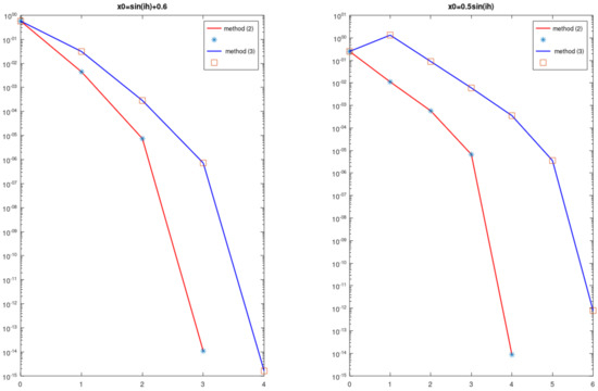
Figure 1 shows $\parallel F\left(x_n\right){\parallel }_{\infty }$ at each iteration. The results are obtained for $m=49$ and $\epsilon ={10}^{-10}$. The starting approximations $x_0$ were given by formulas $x_{0,i}=sin\left(ih\right)+0.6$ (for the graphs on the left) and $x_{0,i}=0.5sin\left(ih\right)$ (for the graphs on the right). Notice that the method (2) convergences faster than (3) for both problems.

Figure 1. Example 2: norm of residual at each iteration.

5. Conclusions

The local convergence analysis of the method (2) and the method (3) previously was given under hypotheses on the seventh derivative on the space ${\mathbb{R}}^i$. The analysis did not provide computable error bounds or uniqueness results for the solution. The rest of the methods listed in the Introduction have the same limitations. We wrote this paper to address these problems and to extend the applicability of these methods. As a sample, we demonstrated that with method (2) and method (3). However, the new approach works on the rest of the aforementioned methods. In particular, we considered the semi-local convergence analysis for these methods which is more interesting and challenging that the local convergence. Computable error estimates as well as the uniqueness of the solution results were given in the more general setting of Banach spaces. Moreover, the convergence is based only on the derivative appearing on the method and $\omega$-continuity conditions. The new approach will be applied in the future to other iterative methods.

References

- Argyros, I.K. The Theory and Applications of Iteration Methods, 2nd ed.; Engineering Series; CRC Press: Boca Raton, FL, USA, 2022. [Google Scholar]
- Shakhno, S.M. Convergence of the two-step combined method and uniqueness of the solution of nonlinear operator equations. J. Comput. Appl. Math. 2014, 261, 378–386. [Google Scholar] [CrossRef]
- Shakhno, S.M. On an iterative algorithm with superquadratic convergence for solving nonlinear operator equations. J. Comput. Appl. Math. 2009, 231, 222–235. [Google Scholar] [CrossRef]
- Argyros, I.K.; Shakhno, S.; Yarmola, H. Two-step solver for nonlinear equation. Symmetry 2019, 11, 128. [Google Scholar] [CrossRef]
- Darvishi, M.T.; Barati, A. A fourth-order method from quadrature formulae to solve systems of nonlinear equations. Appl. Math. Comput. 2007, 188, 257–261. [Google Scholar] [CrossRef]
- Hueso, J.L.; Martínez, E.; Teruel, C. Convergence, efficiency and dynamics of new fourth and sixth order families of iterative methods for nonlinear systems. J. Comput. Appl. Math. 2015, 275, 412–420. [Google Scholar] [CrossRef]
- Jarratt, P. Some fourth order multipoint iterative methods for solving equations. Math. Comp. 1966, 20, 434–437. [Google Scholar] [CrossRef]
- Kou, J.; Li, Y. An improvement of the Jarratt method. Appl. Math. Comput. 2007, 189, 1816–1821. [Google Scholar] [CrossRef]
- Magrenán, Á.A. Different anomalies in a Jarratt family of iterative root-finding methods. Appl. Math. Comput. 2014, 233, 29–38. [Google Scholar]
- Chun, C.; Neta, B. Developing high order methods for the solution of systems of nonlinear equations. Appl. Math. Comput. 2019, 342, 178–190. [Google Scholar] [CrossRef]
- Cordero, A.; Torregrosa, J.R. Variants of Newtons method using fifth-order quadrature formulas. Appl. Math. Comput. 2007, 190, 686–698. [Google Scholar]
- Sharma, J.R.; Guha, R.K.; Sharma, R. An efficient fourth order weighted-Newton method for systems of nonlinear equations. Numer. Algor. 2013, 62, 307–323. [Google Scholar] [CrossRef]
- Sharma, J.R.; Arora, H. Efficient Jarratt-like methods for solving systems of nonlinear equations. Calcolo 2014, 51, 193–210. [Google Scholar] [CrossRef]
- Xiao, X.; Yin, H. A simple and efficient method with high order convergence for solving systems of nonlinear equations. Comput. Math. Appl. 2015, 69, 1220–1231. [Google Scholar] [CrossRef]
- Zhang, J.; Yang, G. Low-complexity tracking control of strict-feedback systems with unknown control directions. IEEE Trans. Autom. Control. 2019, 64, 5175–5182. [Google Scholar] [CrossRef]
- Zhang, X.; Dai, L. Image enhancement based on rough set and fractional order differentiator. Fractal Fract. 2020, 6, 214. [Google Scholar] [CrossRef]
- Ding, W.; Wang, Q.; Zhang, J. Analysis and prediction of COVID-19 epidemic in South Africa. ISA Trans. 2022, 124, 182–190. [Google Scholar] [CrossRef] [PubMed]
Disclaimer/Publisher’s Note: The statements, opinions and data contained in all publications are solely those of the individual author(s) and contributor(s) and not of MDPI and/or the editor(s). MDPI and/or the editor(s) disclaim responsibility for any injury to people or property resulting from any ideas, methods, instructions or products referred to in the content. |
© 2022 by the authors. Licensee MDPI, Basel, Switzerland. This article is an open access article distributed under the terms and conditions of the Creative Commons Attribution (CC BY) license (https://creativecommons.org/licenses/by/4.0/).