Novel MIA-LSTM Deep Learning Hybrid Model with Data Preprocessing for Forecasting of PM_2.5

Abstract

Day by day pollution in cities is increasing due to urbanization. One of the biggest challenges posed by the rapid migration of inhabitants into cities is increased air pollution. Sustainable Development Goal 11 indicates that 99 percent of the world’s urban population breathes polluted air. In such a trend of urbanization, predicting the concentrations of pollutants in advance is very important. Predictions of pollutants would help city administrations to take timely measures for ensuring Sustainable Development Goal 11. In data engineering, imputation and the removal of outliers are very important steps prior to forecasting the concentration of air pollutants. For pollution and meteorological data, missing values and outliers are critical problems that need to be addressed. This paper proposes a novel method called multiple iterative imputation using autoencoder-based long short-term memory (MIA-LSTM) which uses iterative imputation using an extra tree regressor as an estimator for the missing values in multivariate data followed by an LSTM autoencoder for the detection and removal of outliers present in the dataset. The preprocessed data were given to a multivariate LSTM for forecasting PM_2.5 concentration. This paper also presents the effect of removing outliers and missing values from the dataset as well as the effect of imputing missing values in the process of forecasting the concentrations of air pollutants. The proposed method provides better results for forecasting with a root mean square error (RMSE) value of 9.8883. The obtained results were compared with the traditional gated recurrent unit (GRU), 1D convolutional neural network (CNN), and long short-term memory (LSTM) approaches for a dataset of the Aotizhonhxin area of Beijing in China. Similar results were observed for another two locations in China and one location in India. The results obtained show that imputation and outlier/anomaly removal improve the accuracy of air pollution forecasting.

1. Introduction

Almost sixty-eight percent of the total world population is predicted to be settled in cities by 2050. Currently, almost fifty-five percent of the world’s population lives in cities, and it is anticipated that by 2050, sixty-eight percent of the world’s population will be living in cities (https://www.un.org/development/desa/en/news/population/2018-revision-of-world-urbanization-prospects.html (accessed on 1 September 2022)). The migration of the human population to cities impacts cities in multiple ways, one of which is pollution. Urbanization and growth in industrialization cause increases of harmful gases in the atmosphere [1].

Beijing is one of the most polluted cities in China, surrounded by numerous power plants operating on coal. Almost 47 percent of the available coal in the world is consumed by China. This is approximately half of the total consumption of the remaining countries in the world. Some research studies indicate that the city of Ghaziabad in India also has similar pollution problem to Beijing [2].

According to surveys, Ghaziabad is amongst the top five polluted cities in India (https://timesofindia.indiatimes.com/city/lucknow/uttar-pradesh-ghaziabad-2nd-most-polluted-city-in-world-lucknow-ranked-16th/articleshow/90385935.cms (accessed on 1 September 2022)). In this research, datasets from Beijing (China) and Ghaziabad (India) were selected so that the proposed method could be applied and validated.

When the concentration of foreign substances in the air is high enough to negatively impact human health, it is considered to be polluted air. Carbon dioxide (CO₂), nitrogen oxides (NOx), particulate matter (PM), ozone (O₃), carbon monoxide (CO), sulphur dioxide (SO₂), and hydrocarbons (HC) are the major pollutants responsible for pollution. Information about these pollutants was gathered with the help of an ambient information system [3]. Due to the small size of pollutants, fine particulates (particulate matter with an aerodynamic diameter <2.5 mm; PM_2.5) can infiltrate the respiratory system’s bronchioles and alveolar region as well as migrate into blood vessels [4]. PM₁₀ and PM_2.5 are the most dangerous contaminants. Their pollution levels can be used by government organizations and authorities to take preventative measures and necessary action to control and decrease pollution. Predicting PM_2.5 and PM₁₀ concentrations could be of great help to administrations in mitigating the negative consequences of these pollutants. As a result, new approaches for estimating PM_2.5 and PM₁₀ concentrations are always required to be searched for by researchers. Quality of air and weather are inextricably linked with meteorological elements, such as air pressure, humidity, temperature, cloud coverage, wind speed, wind direction, and precipitation, having a significant impact on air quality forecasting. The latest artificial intelligence (AI) techniques are used for forecasting air quality. Moreover, due to increased computational power, many researchers have focused on deep learning techniques in various areas such as image analytics, video analytics, sequential modeling, and data analysis using data-driven models [5]. In various fields, artificial neural networks (ANNs) are also used for detection wherein the data used for analytics must be preprocessed in order to get faithful results [6,7]. Raw data contains missing information and noise which may hamper the end results of any applied techniques.

The research work presented in this paper focuses on a unique hybrid method named the MIA-LSTM method which uses iterative imputation to deal with unavailable values present in the data followed by an LSTM autoencoder to remove noise in the time series data and then predict the PM_2.5 concentration.

The main contributions of this research paper are as follows:

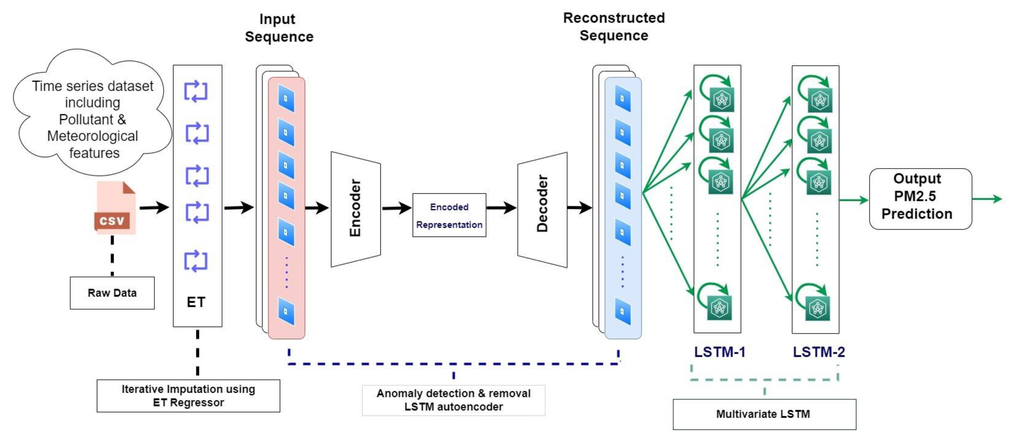
• The use of an effective imputation method for handling missing information in the data by using an iterative method with an extra tree regressor as an estimator for finding replacements for missing fields in multivariate data.
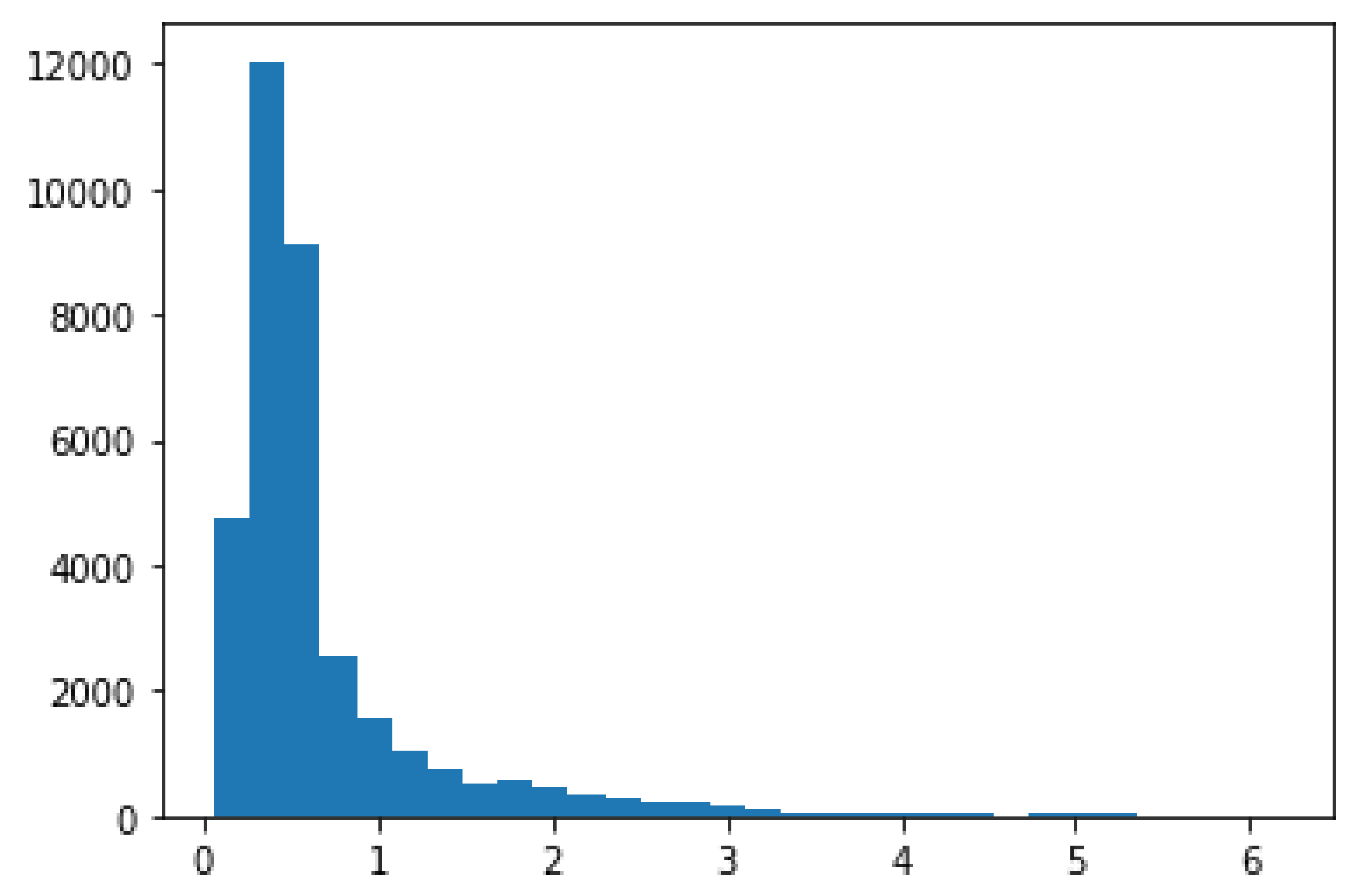
• Anomalies in the data are detected using an autoencoder that uses LSTM for encoding and decoding purposes where the threshold was set on the value of MAE for identifying the anomaly in the dataset
• The proposed MIA-LSTM model that integrates a multivariate iterative imputation method and an autoencoder LSTM predicts PM_2.5 concentration with increased prediction accuracy by adding an extra LSTM layer in the last stage.

2. Related Work

2.1. Missing Values, Imputation, and Forecasting

In data engineering, applications such as air pollution data analysis and prediction and the imputation of missing values are real and inevitable problems [8,9]. As a result, various ways to impute missing data have been developed. Many research papers have been observed where the missing data were removed, and then the analysis is performed on the remaining data. However, it is always vital to replace missing values with some significant values that may improve the performance of the system. Moreover, if the data analysis is performed without replacing missing values, the quality of the data analysis is contentious. The proposed method in this paper takes care of missing values by implementing iterative imputation. Missing data are always lost in its whole and for all time, but an adequate imputation strategy can help to alleviate the problem as much as possible. Missing data are a significant problem in several scientific fields, especially environmental research [10].

Many univariate methods, such as nearest neighbor imputation, linear imputation, and spline imputation, along with multivariate methods, such as self-organizing map imputation, multilayer perceptron imputation, regression-based imputation, and multivariate nearest neighbor imputation, as well as hybrid methods containing combinations of imputation methods were compared and evaluated, which shows that certain multivariate methods for imputation are better choices [11]. Several factors including the pattern of missing data and the type of missing data influence the appropriate technique for dealing with missing data. Simple imputation methods include missing data imputation by either mean, median of the respective column, or replacing the missing value with the proceeding or succeeding value. The authors in [12] interpolated missing values in environmentally contaminated datasets using a single imputation method termed the site-dependent effect method (SDEM) which provides superior imputation than row-mean imputation. The missing values can be imputed using various regression models, such as multiple linear regression or artificial neural network techniques. In [13], it was concluded that for air pollution prediction, the ANN method performed better than the simple regression method, which provides intuition regarding the use of ANN techniques such as iterative imputation.

The vector autoregressive imputation technique (VAR-IM) is a novel approach for imputing missing values in multivariate time series datasets that improves speed and accuracy [14]. If the percentage of missing data is fairly minimal, VAR-IM does not have priority for imputation (less than 10 percent). Out of the various methods used for imputation, singular value decomposition (SVD), the k-nearest neighbor (KNN) method, and the sequential k-nearest neighbor (SKNN) method provide better imputation accuracy for air pollution datasets [15]. In a comprehensive literature survey performed on missing data, it was determined that both the miss forest (iterative imputation method) and k nearest neighbor methods can handle missing values successfully [16]. The missing values were replaced with a linear interpolation method in the preprocessing stage, and then multiple pollutants were predicted using the MS-TCN model, which performed better compared to other baseline models [17]. The state-of-the-art method to impute multivariate data via chained equations [18] and iterative imputation, miss forest, and deep learning approaches [19,20] was used to impute missing data in air quality datasets. In order to deal with missing data in the air quality datasets, multiple data mining techniques [21,22] as well as statistical techniques [23,24] were implemented for appropriate imputation. The missing values were found by building a model based on a complete instance of the dataset excluding missing values; the nonparametric iterative imputation algorithm (NIIA) method as an extension to the solution of imputation using incomplete instances of the dataset was proposed [25]. Ref. [15] compared six imputation models and showed that various KNN imputation methods were superior to simple imputation techniques, such as mean or median imputation techniques. A hybrid imputation method proposed in [26], called KI, is a combination of KNN and iterative imputation and obtained good results compred to a simple KNN method. For NOx prediction, an LSSVM-based iteration strategy was utilized, which improved the accuracy of pollutant prediction while reducing time complexity and ensuring prediction speed and accuracy [27]. The missing values in the simple LSTM model were filled up by zeros, and the author proposed another LSTM model where the missing values were interpolated by Akima’s interpolation [28]. It was proved by imputing missing attribute values that the suggested spatial–temporal (CNN BILSTON-IDW) prediction approach may successfully tackle data imputation challenges for air quality modeling, hinting that further interpolation can be improved using a multivariate dataset [29]. The missing values were replaced with a linear interpolation method in preprocessing stage followed by the prediction of multiple pollutants using the M-ConvLSTM model, which performed better compared with single output models [30]. With the use of the Keras development library, the complexity of RNN implementations has been extensively reduced, enabling noncomputer scientists to use DL without coding overhead [31]. The LSTM model shows satisfactory results and applies to time series challenges, such as forecasting wide area pollution from multiple stations and multiple pollutants. It could effectively predict individual source emissions or model source apportionment under different criteria.

2.2. Outliers, Anomalies, and Forecasting

Multidimensional pollutant data and meteorological data consist of multivariate data which is collected in chronological order from monitoring stations at a particular interval of time. This data has various complications such as dimensional explosions, periodic trends, etc. Due to these problems, simple outlier removal methods result in poor spotting of outliers. Hence, there is a need to remove these outliers/anomalies from the dataset before prediction. There are two types of anomalies in air pollution datasets: unwanted data and others depending on the event of interest. Unwanted data are cleaned by using simple outlier removal methods, such as the inter quartile range, z-score, Grubb’s test, Tietjen–Moore test, and Hampel’s test methods [32]. In later cases, outliers/anomalies have been removed by machine learning-based models, such as KNN, ARIMA, and SVM [33], and deep learning models, such as variational models based on autoencoders [34] and LSTM autoencoders [35]. Detecting anomalies using a combination of the robust projection pursuit and Mahalanobis distance method implemented in [36] showed that anomaly detection is important. Before removing the anomalies in the dataset, the missing values were replaced by a simple column median calculated from available data.

2.3. Modern Methods Used for Forecasting

For the time series data prediction problem, the existing work [37] that uses machine learning methods, such as ANN, does not remember the recurrent past data. However, it is very important to consider past data in time series forecasting. In recent times, time series data RNNs have gained a lot of attention; it is one of the classes of artificial neural networks (ANNs). The first architecture to reveal the hidden structure of data was the Elman RNN [38] where a simple RNN uses BPNN (back propagation through time). This RNN outperforms simple ANNs with feed-forward networks for data that are dynamic in nature [39]. Strength and limitations of forecasting techniques by in various research papers are summarized in

Table 1. Strength and limitations of forecasting techniques.

Reference No	Technique	Preprocessing Method	Strength	Limitations
[28]	CNN-BILSTM-IDW	Linear interpolation for missing values	Deep learning and geostatistical approach obtained better accuracy.	Time complexity is not discussed in the hybrid method.
[49]	LSTM	Missing values ignored	Different LSTM configurations were tested.	Missing values ignored.
[50]	VMD-LASSO-SAE-DESN	VMD and LASSO	Extracted information from high-resolution dataset.	Time complexity is not mentioned.
[53]	Proximity and clustering method	Linear interpolation for missing values	Anomalies detected from air pollution dataset.	Not mentioned.
[55]	LSTM and DAE	Only checked for missing values	LSTM proved slightly better than DAE.	Data preprocessing needs to be taken care of.
[56]	Four different architecture including CNN	Simple imputation of backward fill used for imputation	Data plus images used for pollution prediction.	Requires more computational power.
[57]	Univariate LSTM	Negative values present in dataset were removed	Model performance checked with different batch size.	Calibration part is missing for the deployed device.
[58]	Simple RNN, LSTM, and GRU	Null values are removed	For lower time intervals, LSTM and GRU obtained good accuracy.	Imputation not performed for missing values.
[59]	PCA-Attention-LSTM	Missing values filled with average of adjacent values	Analysis of variable importance was performed.	Time complexity is not mentioned.

.

There are some limitations of RNNs too, as it is incapable of remembering long-term significant important data. Further, whenever there are long-term dependencies, BPNN experiences exploding and vanishing gradient problems. Long Short-Term Memory (LSTM), a further extension to RNN, provides the solution to the above problem.

The state-of-the-art method of LSTM to predict the outbreak of COVID-19 infection is provided in [40], which obtains good prediction accuracy but also concluded that missing values in the data have put limitations in doing a thorough analysis. In this article, preprocessing was performed using a state-space vector using Taken’s theorem, and outliers were treated.

Hybrid methods utilizing LSTM are widely implemented for time series forecasting problems, such as stock prediction [41], which results in improved prediction accuracy [42]. Hybrid versions of LSTM, such as wavelet LSTM, are better in time series prediction compared to the traditional methods used [43]. Trending models for enhanced time series forecasting were proposed in the electrical domain where researchers concluded that a wavelet adaptive neuro-fuzzy inference system outperformed other competent models such as the group method of data handling, LSTM, bootstrap aggregation, sequential learning, and many ensemble learning methods [44]. Recently, many hybrid methods and ensemble learning methods have been applied for time series forecasting problems and provide encouraging results [45]. Out of the many ensemble learning models, random subspace and stacking ensemble models provide better results for prediction. Moreover, compared to LSTM, which takes higher computational power, the proposed ensemble models proved to be better. PM_2.5 concentrations can be forecasted in the future using state-of-the-art ensemble learning methods [46].

A deep learning model, i.e., multivariate LSTM, was used for air quality prediction during the pandemic for short-term and long-term prediction; the bidirectional LSTM outperformed other LSTM models. During this experimentation, missing values were replaced with simple median values, and no comments on outliers and anomalies were stated [47]. Air pollutant concentrations were predicted wth multivariate LSTM; the researchers found that meteorological features play a vital role in the prediction of CO concentrations for PM_2.5 prediction. Meteorological, pollutant, and traffic data were useful, but information regarding imputation and outliers in the preprocessing step was missing [48]. Statistical evidence shows that LSTM grouped by pollutant class (GP-LSTM) and LSTM with individual groups of pollutants as inputs (IGP-LSTM) outperform benchmark algorithms that have been observed. However, these models can still be improved, as LSTMs struggle to detect the presence of sudden high peaks since past information weights on the predictions [49].

In the prediction of air pollutant concentration, many researchers are continuously contributing to the literature by proposing many novel methods; recently, hybrid models have become popular and provide state-of-the-art solutions to prediction problems by extracting useful information from the raw data. When essential information is extracted from data, the VMD (variational mode decomposition) and LASSO (least absolute shrinkage and selector operation) feature selection increase the efficiency of the proposed model [50]. BA-SVR (bat algorithm for support vector regression) is a hybrid algorithm developed with an optimization technique that obtains better results for short-, medium-, and long-term forecasting for the closing price of eighteen indices of the mainland in China [51]. A novel hybrid method was proposed, named ICEEMDAN–MOHHO–ELM (improved complete ensemble empirical mode decomposition with adaptive noise multiobjective Harris hawks optimization extreme learning machine), which first deals with high-frequency noise and achieves stabler and higher predictive performance [52].

To identify abnormalities from air quality data in terms of NO₂ concentrations, the anomaly detection method used a hybrid proximity and clustering-based methodology; before that, missing values were replaced by a linear interpolation method [53]. A new method based on intelligent computing was proposed which uses LSTM and optimization, called a smart air quality prediction model (SAQPM), for the prediction of six types of pollutant prediction, namely PM_2.5, PM₁₀, SO₂, O₃, CO, and NO₂, but did not mention the imputation, and the missing values were dropped [54]. Two models named LSTM and DAE (deep autoencoders) were proposed for predicting PM_2.5 and PM₁₀ values and concluded that LSTM performs better than DAE but did not discuss crucial data preprocessing, such as handling missing values and outliers [55].

Images were used for the prediction of air pollution, and the image features were enhanced by using meteorological data, which has boosted the accuracy of classification [56]. While preprocessing the data, a simple imputation technique of backward fill was used for replacing the missing values in the dataset, but the author agreed that more sophisticated methods for imputation can be used. Univariate LSTM with more batch size is effective in predicting CO concentration [57]. Univariate LSTM and ARIMA comparison showed that ARIMA exhibits better prediction in the case of CO concentration. A relative study considering LSTM, simple RNN, and GRU concluded that simple RNN outperforms the other two in stock market prediction, which is the application of time series data. This is because RNNs are susceptible to vanishing gradient problems [58]. A PCA-attention-LSTM model was used to predict PM_2.5 concentration, which obtained better accuracy compared to LSTM and BPNN models [59]. A novel method was proposed that combines deep learning and a geo-statistical approach, known as CNN-BILSTM-IDW, which increased the prediction accuracy using only past values to predict future values, as the data availability was poor [28]. The authors also suggested that using more data and multivariate interpolation technique prediction could improve results, which is performed in the proposed method.

3. Proposed MIA-LSTM Model

Figure 1 shows the unique methodology which is used in this paper for the prediction of air pollution concentration. The unavailable values from the input data were found and replaced using iterative imputation with an ET regressor as an estimator for calculating the missing values. The output data after imputation contained some anomaly values which were detected and further removed by using LSTM autoencoders by setting the threshold level of MAE. The clean data were then passed through a multivariate LSTM module which predicted the value of PM_2.5 using the previous data of all pollutants and meteorological parameters. Algorithm 1. is the algorithm for proposed MIA-LSTM model.

Algorithm 1. Algorithm for Proposed Method:

1. Input feature1, feature2,→featurex.

2. Output values prediction for PM2.5 based on minimum RMSE/MAE values

[v1 v2 v3]

3. Perform iterative imputation on raw data 4. Input [ f1| f2| ....... fn]

4. Remove the data with missing values

5. Now, split data into two

[f11, f12, f13.....f1n]: without missing values

[f21, f22, f23.....f2n]: missing values

6. for i = 0, where I = iteration

Apply ET regressor on [f11, f12, f13→f1n] by randomly choosing optimal point

7. Impute the data in place of missing values by predicting the values

8. Let

Pvj→predicted values at current level Pvi→predicted values at

α→minimum threshold at previous value for stopping criteria

If Pvj − Pvi <= α,

Then Stop

Else go to step 7 i++

9. Apply LSTM for Anomaly detection

Training set [m1, m2. mn] where m is n dimensional data

Testing set [m’1, m’2. m’n]

Timestamp T = 24

10. On training dataset (Train) calculate reconstructional error using MAE (Threshold

(MAE = max(RE)))

11. On testing dataset (test) Threshold < MAE (test)

Set 1 -> Anomaly

Else

Set 2 -> Normal

12. Now, apply LSTM on normal dataset after removing anomalies Input Train and test

dataset

13. Normalize the normal Dataset into 0-1

14. Choose window size of training data and testing data

15. Train the network N

16. Predict the values of testing data

17. Calculate the Loss using MSE, RMSE, and MAE

End

The following section of the paper provides the detailed explanation of every block used in the MIA-LSTM model.

3.1. Dataset

The dataset used for the experimentations included air pollutants data (hourly) from three nationally controlled air quality monitoring sites in China. The air quality data and meteorological data were collected from twelve AQM sites by the Beijing Municipal Environmental Monitoring Center and China Meteorological Administration [60]. The meteorological data with the air quality data were matched with the closest weather station. Missing data were denoted by NA. The percentage of missing data is also given in the last row of

Table 2. Dataset Description.

Dataset	Beijing Multisite Air Quality Data Dataset	Ghaziabad
Dataset Type	Multivariate	Multivariate
Time Interval	Hourly	Hourly
Monitoring Sites	Aotizhongxin, Gucheng, and Tiantan	Vasundhara, Ghaziabad UPPCB
Monitoring Period	1st March 2013 to 28th February 2017	11 January 2017 to 11 December 2021
Numbers of attributes	18 (row number, year, month, day, hour, PM2.5 concentration (µg/m3), PM10 concentration (µg/m3), SO2 concentration (µg/m3), NO2 concentration (µg/m3), CO concentration (µg/m3), O3 concentration (µg/m3), temperature (degree Celsius), pressure (hPa), dew point temperature (degree Celsius), precipitation (mm), wind direction, wind speed (m/s), name of the air quality monitoring site	13 (datetime, PM2.5 concentration (µg/m3), PM10 concentration (µg/m3), SO2 concentration (µg/m3), NO, NO2 and NOx concentration (µg/m3), CO concentration (µg/m3), Ozone concentration (µg/m3), temperature (degree Celsius), relative humidity, wind speed (m/s), name of the air quality monitoring site
Missing values	Aotizhongxin (9.26%), Gucheng (7.3%), and Tiantan (6.3%)	Vasundhara (15%)

. Another dataset for Ghaziabad city was obtained from the Central Pollution Control Board of India [61]. These data contain all the fields described in Table 2. These data contain hourly values of pollutants and meteorological parameters.

Out of the above attributes available, wind direction was excluded for the prediction purpose from the Chinese dataset, and NOx values were excluded from the Indian dataset. The datasets from both countries contain missing values (the percentage of missing values is given in Table 2 for reference). For the application of various deep learning models, the data were initially split into three sets, i.e., training, validation, and testing, in the ratio of 60%, 20%, and 20%, respectively. The data were divided sequentially as it is time series data.

3.2. Iterative Imputation Using Extra Tree Regressor

The iterative imputation method was used for replacing missing data in the available dataset, where every feature was modeled as a function of other remaining features. The function/model was created with the help of various regressors available. In this process, the missing values were identified using the regressor model and repeated with multiple iterations. This was performed in order to get a more accurate value of the missing data. As many iterations were performed, this process is called iterative imputation. Here, the rows and columns where the missing values were present were identified, and the respective rows were removed. This created two datasets: one which did not contain missing values and the other that contained missing values. The target was to replace these missing values. Using the first set of data and applying the machine learning regression algorithm, the missing values from the later set could be identified. In this paper, during imputation, an extra tree regressor was used to find the missing values. For the same dataset, the experimentation was carried out for the prediction of particulate matter by using various regression techniques, such as LightGBM, gradient boosting regressor, KNN, decision tree, extra tree, and thirteen more. Out of these techniques, extra tree regressor provided the least RMSE and MAE values for prediction. Hence, the ET regressor was chosen as an estimator in the iterative imputation. This was the first iteration; after imputation, the dataset was merged, and after merging the dataset, the regression was applied to obtain the new imputed values. Iterations were carried out until the difference in the imputed values was the least, as shown in the flowchart.

3.3. Anomaly Detection and Removal

Autoencoders have architectural designs such as feed-forward artificial neural networks. Here, one of the hidden layers is a code layer, which has fewer nodes for dimensionality reduction that can be selected by the user. The encoder performs dimensionality reduction whereas the job of the decoder is to get the same output as input (the decoder is a replica image of the encoder).

Autoencoders consist of a decoder and encoder in the output and input layer. When both the encoder and decoder are LSTM modules, then these types of autoencoders are said to be an autoencoder LSTM. Thus, LSTM autoencoders use encoder–decoder LSTM architecture to construct an autoencoder for time series data [62]. An encoder–decoder LSTM is a setup to read an input sequence, replicate it, and recode it for a given dataset of sequences. The model’s ability to replicate the input sequence is used to evaluate its performance. The decoder section of the model can be removed after the model has achieved the necessary degree of performance in replicating the sequence except for the encoder model. The input sequences can then be encoded to a fixed-length vector using this paradigm.

The method used for the determination of anomalies present in a concentration of PM_2.5 analyzed the training data for MAE loss. The reconstruction error threshold was made equal to the maximum MAE loss value found in the training data. The data points were classified in the test set as an anomaly if the reconstruction loss was higher than the reconstruction error threshold value.

Input values were reconstructed by the LSTM autoencoder with MAE values as given in the equations

f_encoder: {xⁿ : t ∈ [1, T ]} → z   t

(1)

f_decoder: z → {xⁿ : t ∈ [1, T ]}

(2)

While applying the proposed method, the meteorological data and pollutant data with n dimensions were transformed by the LSTM model by extracting feature ‘z’: the hidden layer with the ‘z’ dimension (less than the dimension of ’n’). Further in the decoding procedure, using the same time steps of ‘z’, the original data were reconstructed. By this process, the input sequence was taken in time steps from t = 1, 2, 3. ‘x’ was input into fixed-vector ‘z’, which resulted in the model learning about complex temporal correlations between the input variables.

Multivariate LSTM for Forecasting of Particulate Matter

LSTM has a forget gate based on a sigmoid function that helps to discard insignificant information from previous timestamps. The input gate further helps to keep useful information coming from previous timestamps as well as information from the current input of the neuron; it does so by using the sigmoid and tanh functions, respectively. Next is the memory cell, where the forget gate output and input from the input gate are added point-wise, which is responsible for handling long-term dependencies. This memory cell stores meaningful information. Finally, there is an output gate that provides the output to the other neuron by taking the information from the memory cell and the input gate by performing the point-wise operation. Pollutants usually show similar behavioral patterns when studied with respect to time. While applying LSTM, the important information which is used for prediction is stored in the memory cell, and irrelevant information is discarded by forget cell.

For the input LSTM layer used for prediction, the inputs were the pollutant and meteorological data at the tth time instant. The state of the hidden layer at this instant was h_t, which included short-term memory information for the pollutant and meteorological data. The present output was provided by o_t, the internal memory of the cell, and represented by c_t

Each LSTM neuron is represented by the following equations:

Input gate:

$$f_t=\sigma (W_f\left[h_{t-1},x_t\right]+b_f$$

(3)

Forget gate:

$$i_t=\sigma (W_i\left[h_{t-1},x_t\right]+b_i$$

(4)

State update:

$$\widetilde{c_t}=tanh(W_c\left[h_{t-1},x_t\right]+b_c$$

(5)

$$c_t=f_t\ast c_{t-1}+i_t\ast \widetilde{c_t}$$

(6)

Output gate:

$$o_t=\sigma (W_o\left[h_{t-1},x_t\right]+b_o$$

(7)

$$h_t=o_t\ast tanh\left(c_t\right)$$

(8)

$W_f,W_i,W_c,W_o$ represent the weight of the forget gate, input cell state, weight matrix, and output gate.

b_f, b_i, b_o, b_c = corresponding bias

$\tilde{c}$ represents input of cell state to memory cell.

σ represents the sigmoid activation function used by the gates whereas the input and cell state use the tanh function.

4. Evaluation Matrices

For a comparative analysis of the different models, the following evaluation metrics were used: RMSE and R² [63].

Root Mean Square Error:

Information regarding the standard deviation of the forecast error is given by the root mean square error (RMSE) value. The forecasted value spread with respect to the original value is measured by RMSE. The lower the RMSE value, the better the forecast accuracy of any model.

$$RMSE=\surd {{\displaystyle \sum }}_{i=1}^n\frac{{\left(\widehat{y_i}-y_i\right)}^2}{n}$$

(9)

$\widehat{{\mathrm{y}}_{\mathrm{i}}}$ is the forecasted value.

${\mathrm{y}}_{\mathrm{i}}$ is the actual or observed value.

n is the number of observations.

Coefficient of Determination (R²):

“R-squared” is a measure of the goodness of fit of a model. The coefficient of determination is calculated using the following equation.

$$R^2=1-\frac{\sum {\left(\widehat{y_i}-y_i\right)}^2}{\sum {\left(\overline{y_i}-y_i\right)}^2}$$

(10)

$\overline{y_i}$ is the mean of all values of $y$.

5. Results & Discussions

Since the concentration of a 2.5 micron-sized particulate matter depends on certain factors such as the concentration levels of other pollutants, for example, PM₁₀, CO, SO₂, NO₂, O_3, etc., and meteorological factors such as temperature, WSPM, rainfall DEWP, etc., the important factors were identified. Different regressor approaches for forecasting the pollutants, such as a random forest (RF) regressor, light gradient boosting machine (LGBM), gradient boosting (GB) regressor, and decision tree (DT) regressor are applied and discussed in the following section. State-of-the-art time series approaches, such as univariate LSTM, gated recurrent unit, 1D convolutional neural networks, multivariate LSTM, and proposed hybrid methods are also discussed.

5.1. Extra Tress Regressor Usage as an Estimator for Iterative Imputation

Five popular machine learning regressor methods were applied to the datasets of all locations. The train and test sets were split in the ratio of 75% trained and 25% tested. While doing so, if any of the missing values were present, the complete row was eliminated. For the Aotizhonhxin location, the RMSE values for the extra tree regressor, random forest regressor, light gradient boosting machine, gradient boosting regressor, and decision tree regressor are 16.8418, 18.7612, 18.1819, 22.0409, and 27.2191, respectively, with R² values of 0.9560, 0.9455, 0.9488, 0.9250, and 0.8853, respectively as shown in

Table 3. Comparison table for regressor used for deciding estimator in iterative imputation.

	Aotizhonhxin		Gucheng
Model	RMSE	R2	RMSE	R2
Extra Trees Regressor	16.8418	0.9560	18.9825	0.9470
Random Forest Regressor	18.7612	0.9455	20.8966	0.9357
Light Gradient Boosting Machine	18.1819	0.9488	20.0165	0.9410
Gradient Boosting Regressor	22.0409	0.9250	24.9048	0.9086
Decision Tree Regressor	27.2191	0.8853	30.3225	0.8646
	Tiantan		Ghaziabad
Model	RMSE	R2	RMSE	R2
Extra Trees Regressor	16.4132	0.9579	37.8253	0.8812
Random Forest Regressor	17.9955	0.9493	40.8506	0.8615
Light Gradient Boosting Machine	17.0169	0.9546	39.0488	0.8734
Gradient Boosting Regressor	20.7811	0.9325	45.0922	0.8322
Decision Tree Regressor	25.7433	0.8961	58.983	0.7162

. The RMSE and R² values show that the extra tree regressor outperforms the random forest (RF) regressor, light gradient boosting machine (LGBM), gradient boosting (GB) regressor, and decision tree (DT) regressor models. The same is observed for all datasets of all locations. This is the reason we chose the extra tree regressor as the estimator during the imputation of the missing values in the raw data in preprocessing stage.

The dataset used for this experimentation contained missing values for around 7 to 15% of the available data, which was imputed using iterative imputation that used extra tree regression as an estimator as mentioned above.

5.2. Removing Outliers Based on the Values of MAE

The next step in the methodology is to identify the anomalies in the time series dataset; usually, anomalies are where the reconstruction error is large. To check the anomalies, the MAE values on the trained dataset were checked and decided as the threshold. For our dataset, the threshold vale was set to MAE = 1.5, or the threshold can be defined as a 90% value of maximum. Figure 2 shows the graph of the train data MAE values vs. the number of samples. Above the threshold, all the corresponding values in the test dataset were defined as anomalies and removed.

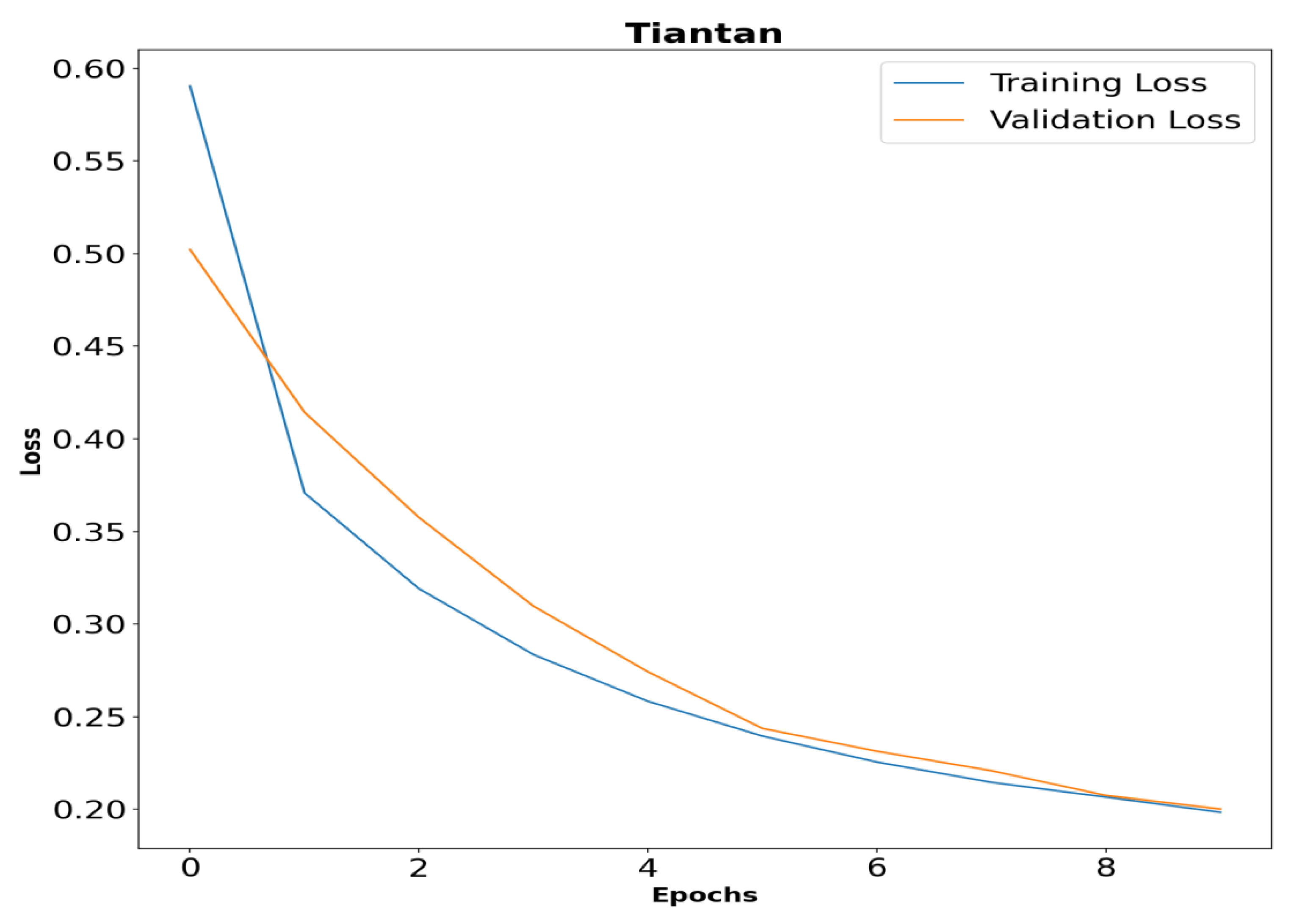
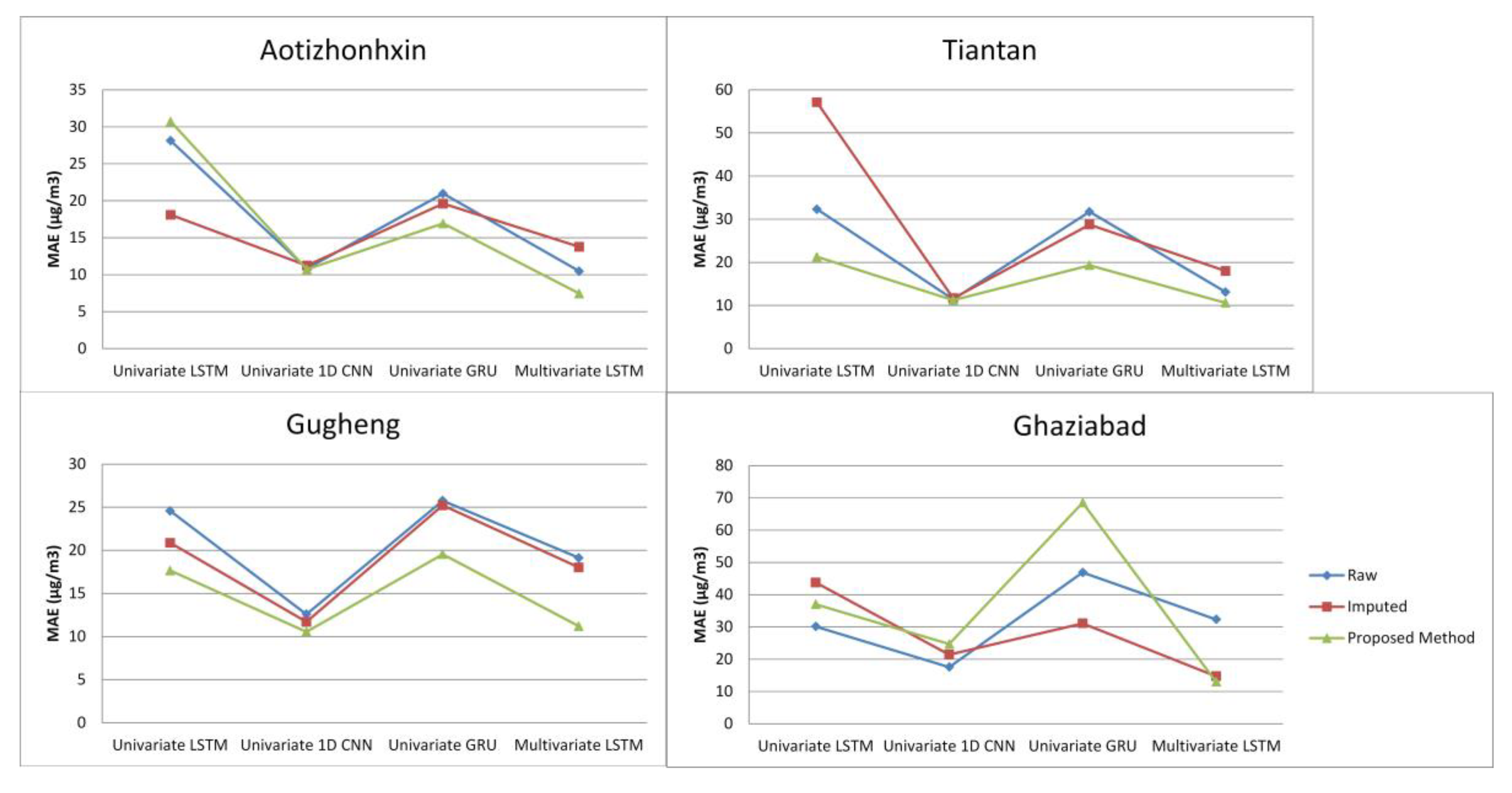
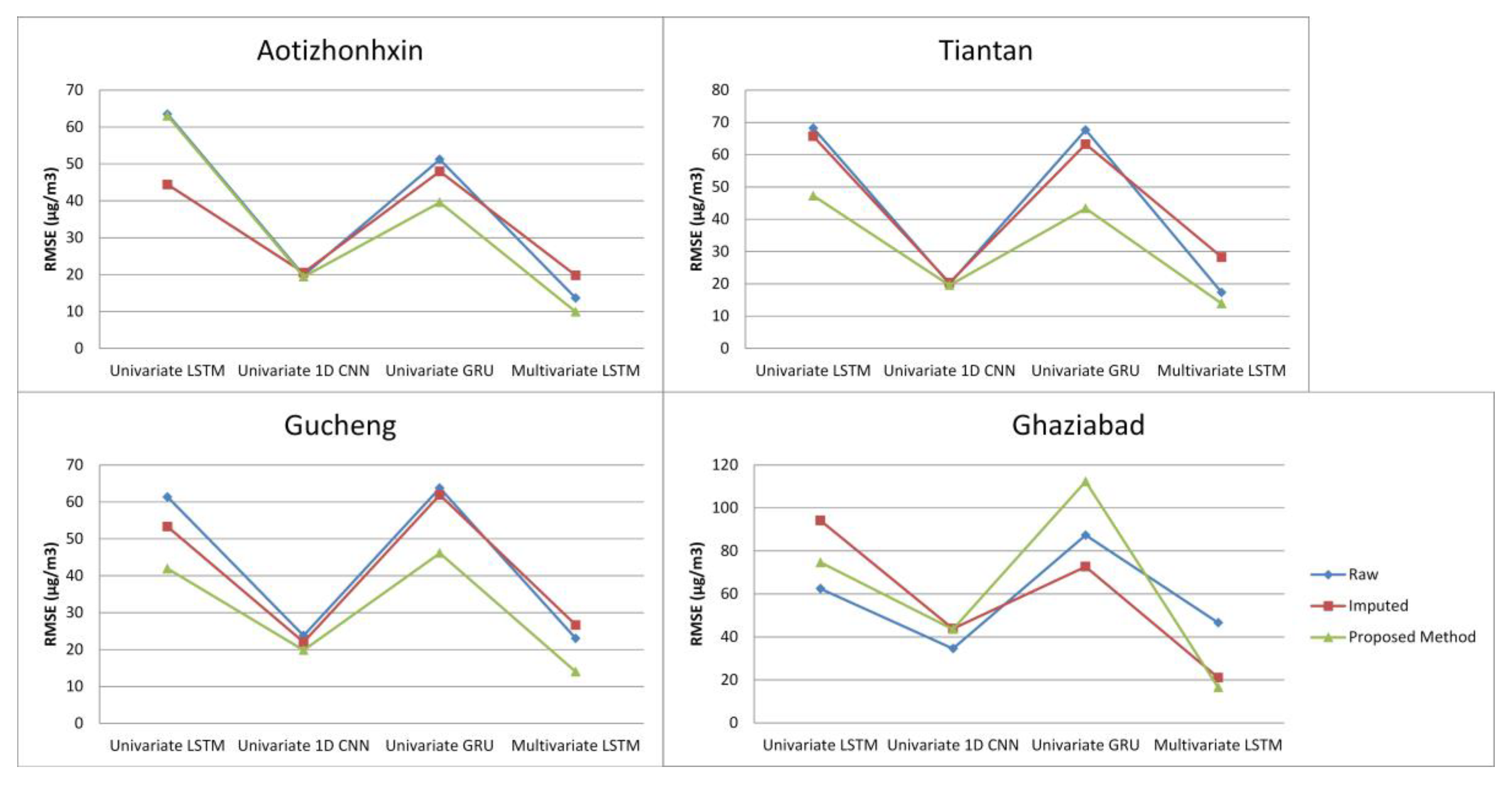
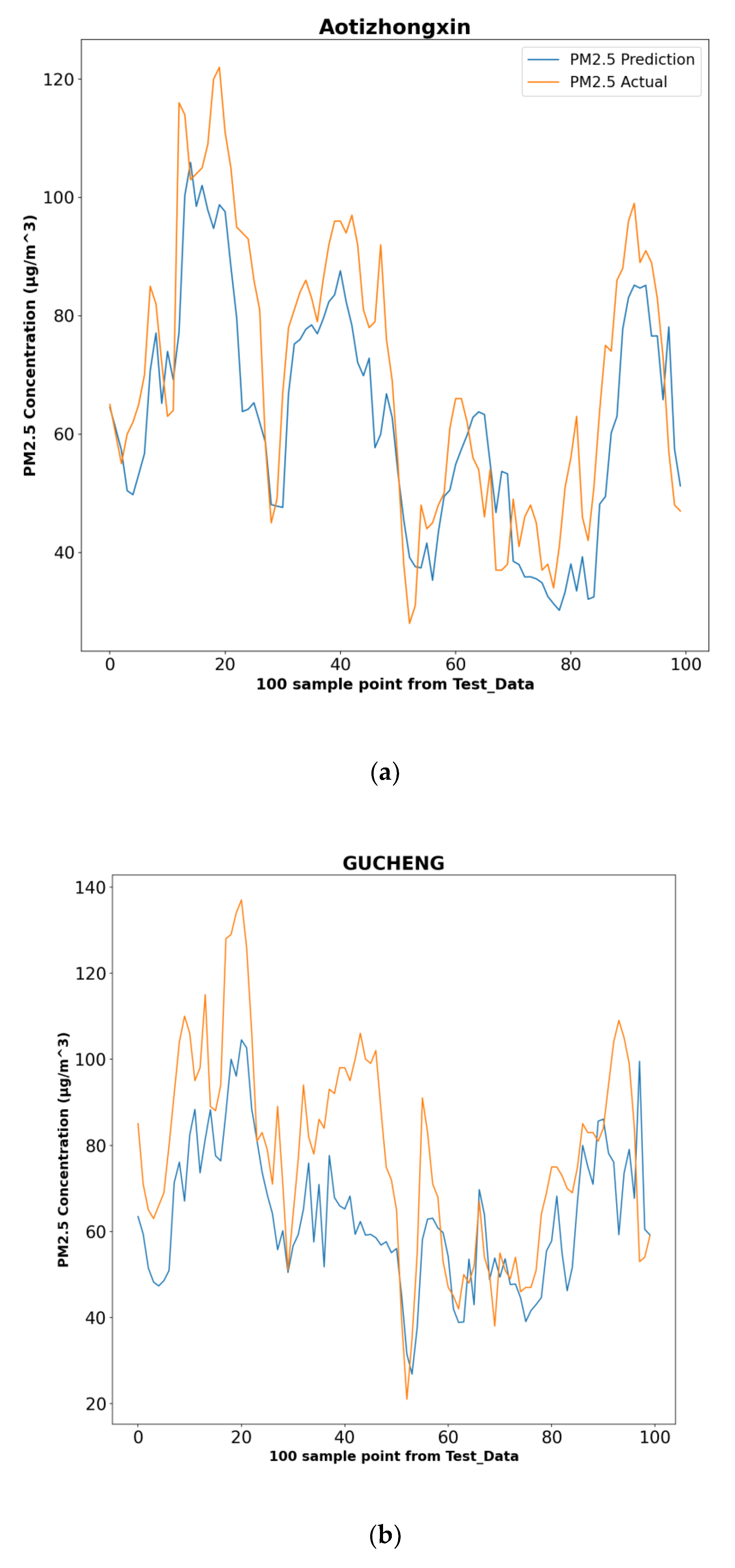
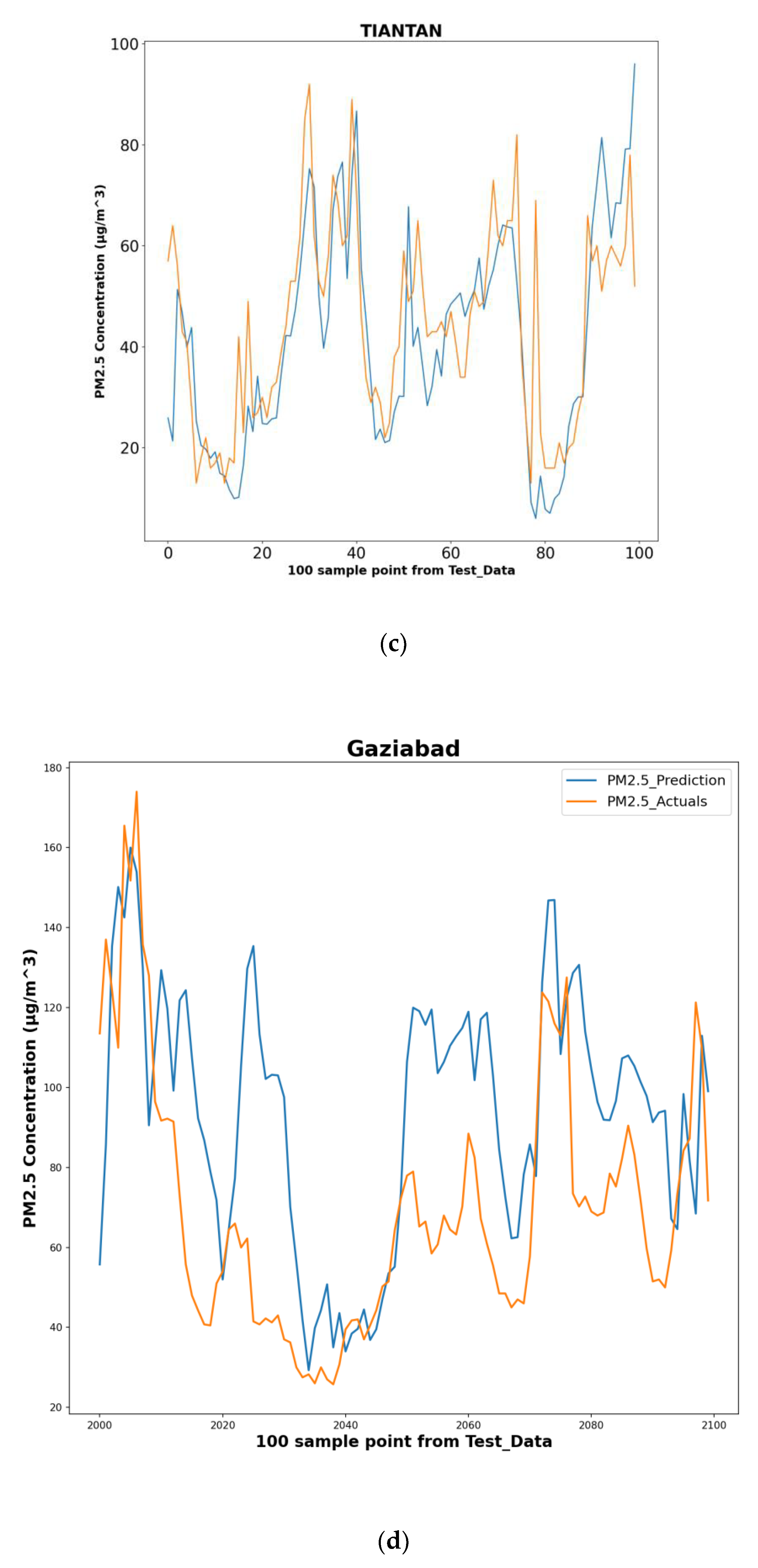
5.3. Performance of Proposed Method

In the experimental setup for all the cases, the multivariate LSTM model at the last stage of prediction has the same number of layers. The relu activation function was used. Based on the experiments performed, the epoch size is limited to 10 epochs in each case, as the error in 10 epochs is low. In Figure 3, a sample graph of the model training and validation curve (loss) is presented. This graph shows the training and validation loss for the Tiantan location dataset. From the graph, it is seen that the training loss and validation loss decrease. It can be concluded from the graph that the proposed model is a good fit for the used dataset.

Table 4. Summary of results of experimentation performed on the dataset of four cities.

	RAW Data (Removed Missing Values)			Imputed Data			Proposed Method
Aotizhonhxin	MAE	RMSE	R2	MAE	RMSE	R2	MAE	RMSE	R2
Univariate LSTM	28.1138	63.4783	0.45535	18.083	44.4132	0.7165	30.6951	63.0365	0.3073
Univariate 1D	10.8385	19.8228	0.9468	11.2217	20.54922	0.9393	10.7215	19.4150	0.9342
Univariate GRU	20.9584	51.2164	0.6454	19.6057	47.97042	0.6692	16.9252	39.5841	0.7268
Multivariate LSTM	10.4696	13.6125	0.7509	13.7667	19.78918	0.8095	7.44549	9.8883	0.8159
Gucheng	MAE	RMSE	R2	MAE	RMSE	R2	MAE	RMSE	R2
Univariate LSTM	24.574	61.329	0.5888	20.867	53.297	0.619	17.653	41.912	0.6882
Univariate 1D	12.586	23.795	0.9381	11.699	22.004	0.9351	10.56	19.832	0.9302
Univariate GRU	25.761	63.746	0.5557	25.227	61.884	0.4863	19.555	46.121	0.6224
Multivariate LSTM	19.12256	23.00376	0.148226	18.0171	26.6355	0.8444	11.1987	13.9660	0.6480
Tiantan	MAE	RMSE	R2	MAE	RMSE	R2	MAE	RMSE	R2
Univariate LSTM	32.311	68.194	0.3872	57.104	65.6630	−0.382	21.272	47.265	0.6202
Univariate 1D	11.431	19.983	0.9474	11.674	20.352	0.9373	11.211	19.567	0.9349
Univariate GRU	31.733	67.657	0.3969	28.747	63.273	0.3939	19.312	43.369	0.6802
Multivariate LSTM	13.10567	17.301	0.8305	18.0027	28.239	0.8054	10.6244	13.884	0.5845
Ghaziabad	MAE	RMSE	R2	MAE	RMSE	R2	MAE	RMSE	R2
Univariate LSTM	30.1511	62.4346	0.4963	43.7731	94.1758	0.4100	37.0318	74.6937	0.4000
Univariate 1D	17.5631	34.6024	0.8453	21.4284	43.8764	0.87194	24.7072	43.5987	0.7955
Univariate GRU	46.8667	87.3550	0.0140	31.1143	72.6943	0.6484	68.5177	112.294	−0.3561
Multivariate LSTM	32.3471	46.6165	0.6351	14.7406	21.0891	0.2630	13.002	16.5374	−0.0237

shows the values for the performance evaluation parameters, namely MAE, MSE, RMSE, and R², for four different models, namely univariate LSTM, univariate 1D CNN, univariate GRU, and multivariate LSTM, for three different scenarios, i.e., with the original data with missing values removed, with IIET imputation, and finally with removed anomaly dataset, respectively.

Each graph shown in Figure 4 and Figure 5 is a visualization of the results and provides the following information: the MAE and RMSE values for each of the four models with the raw (blue), imputed (brown), and proposed method where anomalies were removed (green).

Table 4 shows the results of all experimentations performed for all three locations of Aotizhonhxin, Gucheng, and Tiantan in Beijing. In the case of Aotizhonhxin, it is observed that the RMSE values for the raw data with the missing values removed, with IIET imputed data, and with the proposed data preprocessing method are 13.6125, 19.7891, and 9.8883, respectively; the same is the case with the MAE values which are 10.4696, 13.7667, and 7.4455, respectively. Here, it is observed that the RMSE values and MAE values for the MIA-LSTM method are much smaller compared to the state-of-the-art methods, such as using univariate LSTM, univariate 1D CNN, univariate GRU, and LSTM without data preprocessing. These stated methods with input data without preprocessing can be considered benchmark methods for comparison. These results show the importance of data preprocessing prior to the application of any prediction method. A similar variation is observed for Gucheng and Tiantan locations.

It is clear that the proposed method obtains the best result with the smallest RMSE value among all the methods. For the Gucheng location, the results show that the RMSE values for the raw data with the missing values removal, with IIET imputed data, and with the proposed data preprocessing method are 23.7949, 22.0042, and19.8316, respectively; the case is the same for the MAE values which are 12.5858, 11.6991, and 10.5600, respectively, which shows that prediction error decreases as we preprocess the data initially with imputation and later by removing anomalies. Moreover, the R² value is 0.9302, which is the highest among all the methods, showing that 1D CNN is better in comparison to all regression models in terms of the RMSE value.

Table 4 shows the results for the dataset from Ghaziabad, India. The best results are obtained from the multivariate LSTM model. With the proposed method, the RMSE values for the raw data with the missing values removal, with IIET imputed data, and with the proposed data preprocessing method are 46.6165, 21.0891, and 16.5373, respectively. The case is the same with the MAE values which are 32.3471, 14.7405, and 13.0029, respectively. Although the 1D CNN method was obtaining good predictive results for the dataset of Beijing, with the Ghaziabad dataset, the results are not close to the multivariate LSTM method results; we can say that with more missing data, 1D CNN performance degrades. As mentioned, there was more than 15% of data missing in the Indian dataset; here, imputation plays an important role and can be observed in the better results of the multivariate LSTM prediction compared to using the raw data for prediction with complete rows removed, even if missing values were present. Further removal of anomalies in the imputed dataset using the autoencoder improves the prediction accuracy further and makes it a more reliable system by providing the least error in prediction. Visualization in Figure 4 and Figure 5 makes it clearer. Figure 5 shows a random 100 out of nearly 3000 data points where the predicted and actual values are from the test dataset. It is also seen from Table 4 that for Ghaziabad, the RMSE value for the proposed method is 16.5374, which is quite high compared to the RMSE values of the Aotizhonhxin, Gucheng, and Tiantan location datasets. Moreover, from Table 2, it is clear that the percent of missing values of the Ghaziabad location is higher compared to the remaining three locations.

From Table 4 and Figure 4 and Figure 5, it is observed that 1D CNN works better amongst all three univariate models with a minimum value of MAE and RMSE. Graph of actual versus predicted concentration of PM_2.5 pollutant from sample of 100 points for each location is given in Figure 6. From the results obtained, we can conclude that with imputed data, the error value decreases using the univariate 1D CNN model, which motivates the researcher to handle missing values efficiently.

The results obtained show that the proposed MIA-LSTM model obtains the best result with greatly smaller values of RMSE and MAE in all four graphs. The proposed model performs better, obtaining the smallest value of MAE in all cities from two different countries. This validates that there is a need for data preprocessing prior to applying forecasting methods.

6. Conclusions and Future Scope

Researchers and scientists have developed good models for forecasting air pollution by using various state-of-the-art methods. From the experimental analysis, it is concluded that real-world datasets contain noisy data, and to achieve reliable and accurate forecasting of air pollution, handling of the missing data, outlier detection and removal, and preprocessing steps are of utmost importance. In this paper, these issues are addressed by using powerful data preprocessing steps.

Similarly, effective evaluation measures, i.e., RMSE, MAE, and R², are used to compare and evaluate various prediction models on different datasets. The results show that the ET regressor outperforms other regressors, such as RF, LGBM, GB, and DT, for PM_2.5 prediction. The ET regressor was wisely chosen based on the experimentations for iterative imputation, as demonstrated in Table 3. Different models, such as univariate LSTM, univariate 1D CNN, univariate GRU, and multivariate LSTM, were used for forecasting the hourly value of PM_2.5. All these models were used in three cases: firstly, with raw data where all missing values were removed; secondly, with imputation; and finally, with the removal of anomalies. The proposed forecasting model, i.e., MIA-LSTM, is efficient and effective in predicting PM_2.5 concentration with the smallest error for noisy data. The proposed model shows reduced RMSE and MAE values for all the datasets used, as shown in Table 4.

In the future, the existing work can be extended in the following ways:

• Datasets from different locations with different pollutant concentrations can be harnessed to understand the behavior of air pollution in those particular locations.
• The time complexity is one of the important parameters for forecasting models. Reducing the time complexity without affecting the accuracy of the forecasting can be one of the key aspects of the proposed work.
• More complex models and algorithms, such as an ensemble and CNN-LSTM, can be utilized to further improve the accuracy of air pollution forecasting.

References

1. Yang, Y.; Bao, W.; Li, Y.; Wang, Y.; Chen, Z. Land Use Transition and Its Eco-Environmental Effects in the Beijing–Tianjin–Hebei Urban Agglomeration: A Production–Living–Ecological Perspective. Land 2020, 9, 285. [Google Scholar] [CrossRef]
2. Bagcchi, S. Delhi has overtaken Beijing as the world’s most polluted city, report says. BMJ 2014, 348, g1597. [Google Scholar] [CrossRef] [PubMed]
3. Hazlewood, W.R.; Coyle, L. On Ambient Information Systems: Challenges of Design and Evaluation. In Ubiquitous Developments in Ambient Computing and Intelligence: Human-Centered Applications; IGI Global: Hershey, PA, USA, 2011; pp. 94–104. [Google Scholar] [CrossRef]
4. Jung, C.-R.; Hwang, B.-F.; Chen, W.-T. Incorporating long-term satellite-based aerosol optical depth, localized land use data, and meteorological variables to estimate ground-level PM2.5 concentrations in Taiwan from 2005 to 2015. Environ. Pollut. 2018, 237, 1000–1010. [Google Scholar] [CrossRef] [PubMed]
5. Shaadan, N.; Jemain, A.A.; Latif, M.T.; Deni, S.M. Anomaly detection and assessment of PM10 functional data at several locations in the Klang Valley, Malaysia. Atmos. Pollut. Res. 2015, 6, 365–375. [Google Scholar] [CrossRef] [Green Version]
6. Khadse, C.B.; Chaudhari, M.A.; Borghate, V.B. Conjugate gradient back-propagation based artificial neural network for real time power quality assessment. Int. J. Electr. Power Energy Syst. 2016, 82, 197–206. [Google Scholar] [CrossRef]
7. Pandey, A.; Gadekar, P.S.; Khadse, C.B. Artificial Neural Network based Fault Detection System for 11 kV Transmission Line. IEEE Xplore 2021, 1, 7–136. [Google Scholar] [CrossRef]
8. Allison, P.D. Missing Data. In Sage University Papers Series on Quantitative Applications in the Social Sciences; Sage: Thousand Oaks, CA, USA, 2001; pp. 7–136. [Google Scholar]
9. Little, D.R. Rubin, Statistical Analysis with Missing Data; John Wiley and Sons: New York, NY, USA, 2002. [Google Scholar]
10. Xia, Y.; Fabian, P.; Stohl, A.; Winterhalter, M. Forest climatology: Estimation of missing values for Bavaria, Germany. Agric. For. Meteorol. 1999, 96, 131–144. [Google Scholar] [CrossRef] [Green Version]
11. Junninen, H.; Niska, H.; Tuppurainen, K.; Ruuskanen, J.; Kolehmainen, M. Methods for imputation of missing values in air quality data sets. Atmos. Environ. 2004, 38, 2895–2907. [Google Scholar] [CrossRef]
12. Plaia, A.; Bondi, A. Single imputation method of missing values in environmental pollution data sets. Atmos. Environ. 2006, 40, 7316–7330. [Google Scholar] [CrossRef]
13. Narkhede, G.G.; Hiwale, A.S.; Khadse, C.B. Artificial Neural Network for the Prediction of Particulate Matter (PM2.5). IEEE 2021, 1, 1–5. [Google Scholar] [CrossRef]
14. Bashir, F.; Wei, H.-L. Handling missing data in multivariate time series using a vector autoregressive model based imputation (VAR-IM) algorithm: Part I: VAR-IM algorithm versus traditional methods. IEEE 2016, 1, 611–616. [Google Scholar] [CrossRef]
15. Zainuri, N.A.; Jemain, A.A.; Muda, N. A Comparison of Various Imputation Methods for Missing Values in Air Quality Data. Sains Malays. 2015, 44, 449–456. [Google Scholar] [CrossRef]
16. Wijesekara, W.M.L.K.N.; Wijesekara, L. Liyanage, Comparison of Imputation Methods for Missing Values in Air Pollution Data: Case Study on Sydney Air Quality Index. In Advances in Information and Communication. FICC 2020. Advances in Intelligent Systems and Computing; Arai, K., Kapoor, S., Bhatia, R., Eds.; Springer: Berlin/Heidelberg, Germany, 2020; Volume 1130. [Google Scholar]
17. Samal, K.K.R.; Babu, K.S.; Das, S.K. A Neural Network Approach with Iterative Strategy for Long-term PM2.5 Forecasting. In Proceedings of the 2021 IEEE 18th India Council International Conference (INDICON), Guwahati, India, 19–21 December 2021; pp. 1–6. [Google Scholar]
18. Buuren, S.V.; Groothuis-Oudshoorn, K. Mice: Multivariate Imputation by Chained Equations in R. J. Stat. Softw. 2011, 45, 1–67. [Google Scholar] [CrossRef] [Green Version]
19. Alsaber, A.R.; Pan, J.A. Al-Hurban, Handling Complex Missing Data Using Random Forest Approach for an Air Quality Monitoring Dataset: A Case Study of Kuwait Environmental Data (2012 to 2018). Int. J. Environ. Res. Public Health 2021, 18, 7908071. [Google Scholar] [CrossRef]
20. Kim, T.; Kim, J.; Yang, W.; Lee, H.; Choo, J. Missing Value Imputation of Time-Series Air-Quality Data via Deep Neural Networks. Int. J. Environ. Res. Public Health 2021, 18, 12213. [Google Scholar] [CrossRef]
21. Gessert, G.H. Handling missing data by using stored truth values. ACM SIGMOD Rec. 1991, 20, 30–42. [Google Scholar] [CrossRef]
22. Pesonen, E.; Eskelinen, M.; Juhola, M. Treatment of missing data values in a neural network based decision support system for acute abdominal pain. Artif. Intell. Med. 1998, 13, 139–146. [Google Scholar] [CrossRef]
23. Caruana, R. An non-parametric EM-style algorithm for imputing missing values. In Proceedings of the Eighth International Workshop on Artificial Intelligence and Statistics, Key West, FL, USA, 4–7 January 2001; Morgan Kaufmann: Burlington, MA, USA, 2001; pp. R3:35–R3:40. Available online: https://proceedings.mlr.press/r3/caruana01a.html (accessed on 24 October 2022).
24. Kahl, F. Minimal projective reconstruction including missing data. IEEE Trans. Pattern Anal. Mach. Intell. 2001, 23, 418–424. [Google Scholar] [CrossRef]
25. Zhang, S.; Jin, Z.; Zhu, X. Missing data imputation by utilizing information within incomplete instances. J. Syst. Softw. 2011, 84, 452–459. [Google Scholar] [CrossRef]
26. Fouad, K.M.; Ismail, M.M.; Azar, A.T.; Arafa, M.M. Advanced methods for missing values imputation based on similarity learning. PeerJ Comput. Sci. 2021, 7, 619. [Google Scholar] [CrossRef]
27. Zhai, Y.; Ding, X.; Jin, X.; Zhao, L. Adaptive LSSVM based iterative prediction method for NOx concentration prediction in coal-fired power plant considering system delay. Appl. Soft Comput. 2020, 89, 106070. [Google Scholar] [CrossRef]
28. Chang, Y.S.; Abimannan, S.; Chiao, H.T. An ensemble learning based hybrid model and framework for air pollution forecasting. Environ. Sci. Pollut. Res. 2020, 27, 38155–38168. [Google Scholar] [CrossRef] [PubMed]
29. Samal, K.; Babu, K.; Das, S. Spatio-temporal Prediction of Air Quality using Distance Based Interpolation and Deep Learning Techniques. EAI Endorsed Trans. Smart Cities 2018. [Google Scholar] [CrossRef]
30. Samal, K.K.R.; Babu, K.S.; Das, S.K. Time Series Forecasting of Air Pollution using Deep Neural Net-work with Multi-output Learning. In Proceedings of the 2021 IEEE 18th India Council International Conference (INDICON), Guwahati, India, 19–21 December 2021; pp. 1–5. [Google Scholar]
31. Samal, K.K.; Babu, K.; Panda, A.K.; Das, S.K. Data Driven Multivariate Air Quality Forecasting using Dynamic Fine Tuning Autoencoder Layer. In Proceedings of the 2020 IEEE 17th India Council International Conference (INDICON), New Delhi, India, 10–13 December 2020; pp. 1–6. [Google Scholar]
32. Mahajan, S.; Kumar, B.; Pant, U.K. Tiwari, Incremental Outlier Detection in Air Quality Data Using Statistical Methods. In Proceedings of the 2020 International Conference on Data Analytics for Business and Industry: Way Towards a Sustainable Economy (ICDABI), Sakheer, Bahrain, 26–27 October 2020; pp. 1–5. [Google Scholar]
33. Chen, Z.; Peng, Z.; Zou, X.; Sun, H.; Lu, W.; Zhang, Y.; Wen, W.; Yan, H.; Li, C. Deep Learning Based Anomaly Detection for Muti-dimensional Time Series: A Survey. In Cyber Security; CNCERT 2021; Springer: Berlin/Heidelberg, Germany, 2022; Volume 1506. [Google Scholar]
34. Zhang, C.; Li, S.; Zhang, H.; Chen, Y. VELC: A New Variational AutoEncoder Based Model for Time Series Anomaly Detection. arXiv 2019, arXiv:1907.01702. [Google Scholar] [CrossRef]
35. Provotar, O.I.; Linder, Y.M.; Veres, M.M. Unsupervised Anomaly Detection in Time Series Using LSTM-Based Autoencoders. In Proceedings of the 2019 IEEE International Conference on Advanced Trends in Information Theory (ATIT), Kyiv, Ukraine, 18–20 December 2019; pp. 513–517. [Google Scholar]
36. Shogrkhodaei, S.S.Z.; Razavi-Termeh, A.V. Fathnia, Spatio-temporal modeling of PM2.5 risk mapping using three machine learning algorithms. Environ. Pollut. 2021, 289, 117859. [Google Scholar] [CrossRef] [PubMed]
37. Pun, T.B.; Shahi, T.B. Nepal Stock Exchange Prediction Using Support Vector Regression and Neural Networks. In Proceedings of the 2018 Second International Conference on Advances in Electronics, Computers and Communications (ICAECC), Bangalore, India, 9–10 February 2018; pp. 1–6. [Google Scholar] [CrossRef]
38. Elman, J.L.; Zipser, D. Learning the hidden structure of speech. J. Acoust. Soc. Am. 1988, 83, 1615–1626. [Google Scholar] [CrossRef] [Green Version]
39. Omlin, C.; Thornber, K.; Giles, C. Fuzzy finite-state automata can be deterministically encoded into recurrent neural networks. IEEE Trans. Fuzzy Syst. 1998, 6, 76–89. [Google Scholar] [CrossRef]
40. Chandra, R.; Jain, A.; Chauhan, D.S. Deep learning via LSTM models for COVID-19 infection forecasting in India. PLoS ONE 2022, 17, e0262708. [Google Scholar] [CrossRef]
41. Shahi, T.B.; Shrestha, A.; Neupane, A.; Guo, W. Stock Price Forecasting with Deep Learning: A Comparative Study. Mathematics 2020, 8, 1441. [Google Scholar] [CrossRef]
42. Ahmed, D.M.; Hassan, M.M.; Mstafa, R.J. A Review on Deep Sequential Models for Forecasting Time Series Data. Appl. Comput. Intell. Soft Comput. 2022, 2022, 6596397. [Google Scholar] [CrossRef]
43. Branco, N.W.; Cavalca, M.S.M.; Stefenon, S.F.; Leithardt, V.R.Q. Wavelet LSTM for Fault Forecasting in Electrical Power Grids. Sensors 2022, 22, 8323. [Google Scholar] [CrossRef]
44. Neto, N.F.S.; Stefenon, S.F.; Meyer, L.H.; Ovejero, R.G.; Leithardt, V.R.Q. Fault Prediction Based on Leakage Current in Contaminated Insulators Using Enhanced Time Series Forecasting Models. Sensors 2022, 22, 6121. [Google Scholar] [CrossRef]
45. Cawood, P.; Van Zyl, T. Evaluating State-of-the-Art, Forecasting Ensembles and Meta-Learning Strategies for Model Fusion. Forecasting 2022, 4, 732–751. [Google Scholar] [CrossRef]
46. Stefenon, S.F.; Ribeiro, M.H.D.M.; Nied, A.; Yow, K.-C.; Mariani, V.C.; Coelho, L.D.S.; Seman, L.O. Time series forecasting using ensemble learning methods for emergency prevention in hydroelectric power plants with dam. Electr. Power Syst. Res. 2021, 202, 107584. [Google Scholar] [CrossRef]
47. Tiwari, A.; Gupta, R.; Chandra, R. Delhi air quality prediction using LSTM deep learning models with a focus on COVID-19 lockdown. arXiv 2021, arXiv:2102.10551. [Google Scholar] [CrossRef]
48. Karroum, K.; Lin, Y.; Chiang, Y.-Y.; Ben Maissa, Y.; El Haziti, M.; Sokolov, A.; Delbarre, H. A Review of Air Quality Modeling. Mapan 2020, 35, 287–300. [Google Scholar] [CrossRef]
49. Navares, R.; Aznarte, J.L. Predicting air quality with deep learning LSTM: Towards comprehensive models. Ecol. Inform. 2019, 55, 101019. [Google Scholar] [CrossRef]
50. Xu, Y.; Liu, H.; Duan, Z. A novel hybrid model for multi-step daily AQI forecasting driven by air pollution big data. Air Qual. Atmos. Health 2020, 13, 197–207. [Google Scholar] [CrossRef]
51. Zheng, J.; Wang, Y.; Li, S.; Chen, H. The Stock Index Prediction Based on SVR Model with Bat Optimization Algorithm. Algorithms 2021, 14, 299. [Google Scholar] [CrossRef]
52. Du, P.; Wang, J.; Hao, Y.; Niu, T.; Yang, W. A novel hybrid model based on multi-objective Harris hawks optimization algorithm for daily PM2.5 and PM10 forecasting. Appl. Soft Comput. 2020, 96, 106620. [Google Scholar] [CrossRef]
53. Aggarwal, A.; Toshniwal, D. Detection of anomalous nitrogen dioxide (NO2) concentration in urban air of India using proximity and clustering methods. J. Air Waste Manag. Assoc. 2019, 69, 805–822. [Google Scholar] [CrossRef] [PubMed]
54. Al-Janabi, S.; Mohammad, M.; Al-Sultan, A. A new method for prediction of air pollution based on intelligent computation. Soft Comput. 2019, 24, 661–680. [Google Scholar] [CrossRef]
55. Xayasouk, T.; Lee, H.; Lee, G. Air Pollution Prediction Using Long Short-Term Memory (LSTM) and Deep Autoencoder (DAE) Models. Sustainability 2020, 12, 2570. [Google Scholar] [CrossRef] [Green Version]
56. Kalajdjieski, J.; Zdravevski, E.; Corizzo, R.; Lameski, P.; Kalajdziski, S.; Pires, I.; Garcia, N.; Trajkovik, V. Air Pollution Prediction with Multi-Modal Data and Deep Neural Networks. Remote. Sens. 2020, 12, 4142. [Google Scholar] [CrossRef]
57. Spyrou, E.D.; Tsoulos, I.; Stylios, C. Applying and Comparing LSTM and ARIMA to Predict CO Levels for a Time-Series Measurements in a Port Area. Signals 2022, 3, 235–248. [Google Scholar] [CrossRef]
58. Dey, P.; Emam, H.; Md, H.; Mohammed, C.; Md, A.; Andersson, H.K.M. Comparative Analysis of Recurrent Neural Networks in Stock Price Prediction for Different Frequency Domains. Algorithms 2021, 14, 251. [Google Scholar] [CrossRef]
59. Ding, W.; Zhu, Y. Prediction of PM2.5 Concentration in Ningxia Hui Autonomous Region Based on PCA-Attention-LSTM. Atmosphere 2022, 13, 1444. [Google Scholar] [CrossRef]
60. Chen, S.X. Beijing Multi-Site Air-Quality Data Data Set. 2018. Available online: https://archive.ics.uci.edu/ml/datasets/Beijing+Multi-Site+Air-Quality+Data (accessed on 1 March 2022).
61. CPCB. Air Pollution. 2022. Available online: https://cpcb.nic.in/air-pollution. (accessed on 10 March 2022).
62. Nguyen, H.; Tran, K.; Thomassey, S.; Hamad, M. Forecasting and Anomaly Detection approaches using LSTM and LSTM Autoencoder techniques with the applications in supply chain management. Int. J. Inf. Manag. 2020, 57, 102282. [Google Scholar] [CrossRef]
63. Mishra, B.; Shahi, T.B. Deep learning-based framework for spatiotemporal data fusion: An instance of Landsat 8 and Sentinel 2 NDVI. J. Appl. Remote. Sens. 2021, 15, 034520. [Google Scholar] [CrossRef]
Figure 1. MIA-LSTM model.
Algorithms 16 00052 g001
Figure 2. Train data MAE values (x-axis) vs. number of samples (y-axis).
Algorithms 16 00052 g002
Figure 3. Sample graph of training and validation curve for Tiantan location dataset.
Algorithms 16 00052 g003
Figure 4. Graphs showing MAE values for all experimentations.
Algorithms 16 00052 g004
Figure 5. Graphs showing RMSE values for all experimentations.
Algorithms 16 00052 g005
Figure 6. (ad): Graph of actual versus predicted concentration of PM2.5 pollutant from sample of 100 points for each location.
Algorithms 16 00052 g006aAlgorithms 16 00052 g006b