Abstract
We optimize the assignment of transporters to several jobs. Each job consists of processing a large, decomposable volume. A fleet of transporters is given, each of which can only process a limited volume at a time. After processing its share, a transporter must rest for a short time before being able to process another part. This time is only dependent on the assigned job, not on the transporter. Other transporters can take over the processing while a transporter rests. Transporters assigned to the same job wait for their turn in a queue. A transporter can only be assigned to one job. Our goal is to simultaneously minimize the maximum job completion time and the number of assigned transporters by computing the frontier of Pareto optimal solutions. In general, we show that it is NP-hard in the strong sense to compute even a single point on the Pareto frontier. We provide exact methods and heuristics to compute the Pareto frontier for the general problem and compare them computationally.
1. Introduction
In many farming or construction processes, transporter resources are used to carry material to or from the operation site in a cyclic fashion. Examples for such applications are tractors collecting silage from a forage harvester, dump trucks getting filled with excavated earth, or cement or asphalt being fed from trucks to construction sites. Transporters are available on site for a limited amount of processing time, dependent on the loading capacity of the transporter and the processing speed of the main resource.
After that, they have to unload/reload material in some central hub (e.g., a harvest silo, asphalt producer, etc.) before returning to the processing site. The time of absence depends on the distance between the operation site and the hub, but it is the same for all transporters assigned to the same site. Multiple transporters may be assigned to the same working site, so that processing can continue even when some transporters are on-road toward/from the central hub. If no other transporter is available on site, the main work has to pause until the next transporter arrives back on site. Two transporters may not be used for on-site processing at the same time.
This kind of transporter setting is referred to by Jensen et al. [1] as capacitated field operations. Many instances of these types of processes have been studied in the literature from different angles, with different goals, and for different applications, see [1,2,3,4,5,6,7,8]. Recent reviews are provided in [9,10]. The important common feature of all these use cases is that the total volume that needs to be processed on site is usually much larger than the capacity of a single transporter. Figure 1 illustrates such a process for the example of farming.
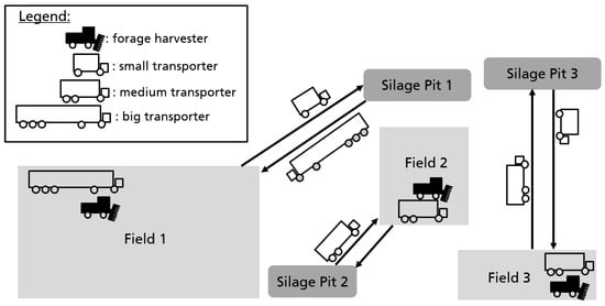
Figure 1.
Example of three fields being harvested by forage harvesters and eight transporters of heterogeneous sizes. Field 1 is assigned an extra transporter due to its large size, making the avoidance of idle times even more important. Field 3 is assigned an extra transporter because it is far away from its silage pit, causing assigned transporters to waste a lot of time on the road.
Since, usually, this type of problem is NP-hard (not solvable in polynomial time unless , see [11]) when viewed as a whole (see [5]), authors turn to mathematical programming formulations (see [2,5,12]) or (meta-)heuristics (see [4,5]).
In this paper, instead, we do not consider the problem as a whole but instead investigate one specific, important sub-problem, namely the assignment of transporters to operation sites. This problem gives rise to an interesting, new scheduling problem, which, to the best of our knowledge, has not been studied in the literature before.
1.1. Formal Problem Definition
For the purpose of this study, we assume that each operation site is assigned exactly one main resource. Otherwise, we split an operation site into multiple neighboring sites, one for each resource assigned. Furthermore, we assume that the processing speed of the main resources is fixed. This is reasonable for tactical planning if the tasks conducted at each site as well as the resources used to do so are similar.
Formally, a set of jobs = is given, each representing one operation site together with a main resource. Furthermore, let = be the set of transporters. In normal scheduling terminology, the transporters would be called resources or machines; however, we stay with the term transporters throughout this paper in order to stay closer to the terminology in our field of application.
Each job has a certain volume that needs to be processed before the job is complete, and each transporter has a certain capacity that can be used up before the transporter has to rest (travel to the central hub). Since we assume the processing speed of the main resources to be fixed, we can translate all volumes into time values for ease of notation. Thus, each job has a saturated processing time , which is the total time it needs to be processed by transporters before it is complete. Similarly, each transporter has a filling time , which is the time it can process a job before it needs to rest. Finally, we denote by the return time of every transporter assigned to job j. In this paper, we do not allow a transporter to be assigned to multiple jobs. Figure 2 shows how two transporters may process the same job.
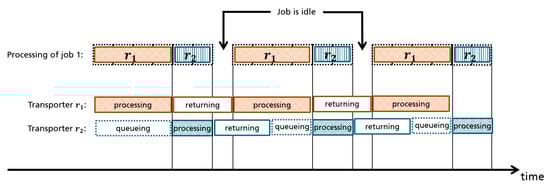
Figure 2.
Example of two transporters relaying each other to process a job. The job processing stops while both transporters are in their return time.
We assume all jobs start processing at the same time. The completion time of a job is given as the sum of and all idle times happening during the processing of job j due to no transporter being available. In particular, is the completion time of job j if job j is never idle (always has a transporter available for processing). Our goal is to minimize the maximum completion time of any job, which is also called the makespan . A short makespan is desirable, because it ties in directly with several crucial performance indicators, such as the necessary opening times of the hub, potential overtime pay for workers, as well as minimizing the time frame in which problems (e.g., due to weather) may happen. In addition, a large makespan may indicate unnecessary idle times for the main resources, which are to be avoided in order to operate cost efficiently.
However, it may not be possible to hire enough transporters to avoid all idle times (due to transporter availability), or, if it is possible, it may still not be economically desirable (due to drivers’ wages) in cases where an additional transporter would only decrease the idle time by a marginal value. Thus, the total number of assigned transporters is another important measure for the quality of a solution. Therefore, our goal in this paper is to jointly minimize the makespan of multiple simultaneously operated sites and minimize the number of used transporters. The problem of assigning transporters to jobs in order to minimize simultaneously the makespan and the number of assigned transporters is called the transporter allocation problem or for short.
As the two objectives of are conflicting, our goal is to find all Pareto optimal solutions. A feasible solution to is Pareto optimal if every other feasible solution with smaller makespan uses a larger number of transporters, and every other feasible solution that uses a smaller number of transporters has a larger makespan. The set of all Pareto optimal solutions is called the Pareto frontier. We refer to [13] for a general introduction to multicriteria optimization.
In the Appendix A, we prove that given a set of transporters assigned to some job , the completion time of j can be estimated by
where
and
The estimate depends on the practical assumption, mentioned above, that jobs are very large compared to transporter capacities and return times. See Theorem A1 for details. We also call the period length and the idle time per period of job j, according to the statements of Lemma A2 in the Appendix A. For the remainder of this paper, we do not deal with the exact scheduling and sequencing of transporters when processing jobs and instead only focus on the assignment of transporters to jobs using Equation (1) to estimate the completion times of the jobs. Therefore, a solution to is fully given by an assignment of transporters to jobs, which are encoded by variables in the following way:
For a solution , we denote by the number of transporters assigned to j under assignment :
In addition, by , we denote the total number of transporters assigned by assignment , i.e.,
Furthermore, we denote by , and the makespan, completion time of job , its period length, and its idle time per period, under solution , respectively. If there is no confusion about the solution referred, we may instead leave out as before.
Note that all mathematical notation introduced in this section and throughout the remainder of the paper is also given again in a concise list in the Abbreviations section at the end of this paper.
Finally, a solution saturates a job if job j has no idle time under solution , that is if and . If solution saturates all jobs , then is called saturating. Recall that in this case, the completion time of every job j is at its minimum value . Note that a saturating solution minimizes both the maximum and total completion time of all jobs. An instance of problem is saturated if there exists at least one saturating assignment.
The remainder of this paper is structured as follows. To finish Section 1 below, we briefly summarize our results and contributions. Then, in Section 2, we present a review of the literature related to our problem. In Section 3, we state and prove some structural properties of , in particular that is NP-hard. In Section 4, we consider the special case where transporters are identical. In Section 5, we discuss the restricted problem of finding saturated solutions, where adding a transporter cannot further decrease any completion time. Our single objective is to minimize the the number of transporters. In Section 6, we develop algorithms to compute a Pareto frontier for the general problem, using results from the saturated problem. We present simulation results in Section 7. Finally, in Section 8, we conclude our paper.
1.2. Our Results
As mentioned before, to the best of our knowledge, this is the first paper to study the problem as presented here explicitly. We show that computing even a single point on the Pareto front for an instance of problem is, in general, NP-hard in the strong sense. It remains NP-complete in the strong sense even if all jobs have the same return time and/or saturated processing time.
In terms of positive results, we show that the minimum number of transporters needed to saturate a job can be computed in time for all jobs. Furthermore, if all transporters are identical, then the whole Pareto front to solve problem can be computed in time. In that case, a single point on the Pareto front can also be computed in time, where denotes the processing time of a job when exactly one transporter is assigned to it. This time complexity may in some cases be better as is no longer part of the estimate. See also Table 1 for an overview of our complexity results.

Table 1.
Overview of complexity results for problem . Note that denotes the case where all return times are identical and denotes the case where all transporter capacities are identical. Finally, denotes the completion time of job j when exactly one transporter is assigned to it, in the case where all transporters have identical capacity.
In addition to these complexity results for sub-problems and special versions, we also consider how to solve the general problem. We suggest several approaches using mathematical programming, heuristics, and combinations of both. We evaluate all suggested algorithms experimentally and discuss their advantages and disadvantages when compared to each other.
2. Literature Review
In this section, we outline how the transporter allocation problem studied in this paper ties in with the wider literature. As mentioned before, to the best of our knowledge, has not been studied in this form before. However, there are several optimization problems that bear a resemblance to . Below, we focus on the two most closely related problems, namely divisible load scheduling, which can be seen as a version of where transporters may process the job in parallel rather than in sequence, and multiple knapsack problems, which relate to in the way that for each job, there is an upper limit of transporter sizes before adding more transporters no longer improves anything. We compare the problems to and explain which, if any, results can be transferred to our setting.
We will not consider papers discussing capacitated field operations in general again, as in the beginning of Section 1, since other than providing the wider practical motivation, they have little relevance for . Furthermore, note that even though both problems stem from logistic tasks, is not comparable to vehicle routing problems. In vehicle routing problems [14], each transporter is usually assigned several delivery jobs, while for , each job is assigned several transporters. Due to this fundamental difference, even though the problems may look related in practice, they are not close from a mathematical perspective.
2.1. Divisible Load Scheduling
In divisible load scheduling [15], a processing load needs to be divided onto several processors, just like the total volume of a job in needs to be divided onto several transporters. The main difference between the two is that in divisible load scheduling, the processors are assumed to be parallel, such that they are allowed to process different parts of the main load at the same time. In addition, usually, in divisible load scheduling problems, only a single load needs to be split across processors, while for , multiple loads need to be assigned to transporters. Note that without any further assumptions, splitting a load over parallel processors is usually easy. Therefore, the literature considers many additional parameters, such as setup times, communication delays between processors, and more complex processor networks (e.g., where sub-processors on the first level have again several second-level sub-processors to which they can divide their sub-task). We refer to [16] for a review. In comparison, as we show in this paper, is much harder, even without any additional assumptions.
Interestingly, many papers consider bi-criteria versions of divisible load scheduling, where the goal is to minimize the makespan and cost of a schedule simultaneously; see [17,18,19]. Here, cost is usually defined as a function of the load assigned to each processor, together with a fixed cost to activate each used processor in the first place [19]. Special versions have been studied without any additional restrictions and where only the fixed cost for each processor is used [17,19]. Note that this version is very close to with only three differences: first, of course, for the divisible load scheduling problem, the processors work in parallel, whereas for , they in sequence; second, in the divisible load scheduling problem, processors may have different speeds but have no maximum load, whereas in , all transporters have the same speed but a maximum capacity after which they must rest; third, for , we assume additionally that the fixed cost for each transporter is the same. This special version of divisible load scheduling is shown to be NP-hard in the usual sense [17]. We prove later that is NP-hard in the strong sense. Furthermore, note that if in the divisible load scheduling problem the fixed cost of all processors is the same, then the NP-hardness proof from [17] is no longer valid, while this assumption holds by definition for .
Most other results for divisible load scheduling are not comparable to either due to additional restrictions for the divisible load scheduling problem or because of the difference in sharing load in parallel or sequential. Thus, techniques used to solve divisible load scheduling problems cannot be easily transferred to .
2.2. Multiple Knapsack Problems
Even though it is not immediately obvious from a practical point of view, is rather strongly related to multiple knapsack problems. Recall that the knapsack problem [20] is a popular optimization problem, with the objective to select items with maximum total value without exceeding a certain capacity. The multiple knapsack problem considers several knapsacks with potentially different capacities. The objective is to assign items to knapsacks such that the total items value is maximized without exceeding any knapsack capacity. In comparison, for , consider each job as a knapsack with a capacity given by the total size of transporters needed before all idle times vanish (note that this capacity is not fixed, as it depends on the largest transporter assigned, cf. Equation (2)). Then, a good allocation of transporters is one where each “knapsack” is as close to exactly filled as possible.
Many knapsack-related problems are known to be NP-hard [11]. Most algorithms for the multiple knapsack problem are either greedy or meta-heuristics such as in [21,22], polynomial approximation schemes such as in [23,24], or exact methods using mathematical programming as in [25,26].
For our paper, a special kind of knapsack problem studied in [27] is of particular interest. In this version, so-called assignment restrictions are given, such that each item is only allowed to be assigned to as subset of the knapsacks. This is interesting, since in , jobs may become ineligible for further transporters once they have reached their minimum possible completion time. In [27], the authors propose several approximation algorithms, some with a simple, greedy structure. We will later (cf. Section 5) see that two of these algorithms can be adjusted to work well as heuristics for .
3. Structural Results
In this section, we consider the structural properties of before turning to solution methods for the general problem and special cases in the remainder of the paper. In the first part of this section, we show that is NP-hard in the strong sense. In the second part of this section, we introduce lower bounds on the number of transporters needed for a job to be saturated, i.e., have no idle time. We also provide an easy algorithm to compute all such lower bounds for a general instance of .
3.1. NP-Hardness of
Unfortunately, is NP-hard in the strong sense, i.e., not solvable in time polynomial in the size of the input, even if the input is encoded in unary encoding, unless , cf. [11]. In fact, we prove below that for an instance of it is, in general, strongly NP-hard to compute even a single point on the Pareto frontier. Let be the decision version of with target makespan . That is, given an instance of and a target makespan , the task for is to decide if there exists an assignment of transporters to jobs such that the makespan is at most , and at most, transporters are used.
Theorem 1.
is NP-complete in the strong sense, even if is chosen as the minimum possible makespan, i.e., . Moreover, it remains NP-complete in the strong sense, even if all jobs have the same return time and/or saturated processing time. Finally, it remains NP-complete in the strong sense even if it reduces to the decision if a saturating assignment exists, i.e., with parameters and .
Proof.
Reduction from three-partition problem, which is NP-complete in the strong sense [11]: Given a multiset S of positive integers, can S be partitioned into m triplets , such that the sum of the numbers in each subset is equal?
The subsets , must form a partition of S in the sense that they are disjoint and they cover S. Let B denote the (desired) sum of each subset , or equivalently, let the total sum of the numbers in S be . The three-partition problem remains strongly NP-complete when every integer in S is strictly between and .
Let (I) be an arbitrary instance of three-partition with and and .
Let M be an arbitrary large positive integer with . Let be the multiset defined by with K being the multiset with . Hence, . In the following, we refer to the elements from K as the large elements. Define now an instance of with the set of resources with filling times . The job set has cardinality m and the return times and saturated processing times for all jobs . Note that, by construction, all jobs have the same return time and the same saturated processing time.
We need to prove the following:
⇒: Given a solution (i.e., a set of triplets with the desired properties) to the three-partition instance (I), we can easily construct a solution to by first assigning the transporters with the filling times corresponding to to the job . Then, each job is additionally assigned to two of the transporters of size M. Since by definition , the return time of is covered exactly by the four smallest elements, meaning each job is saturated and no idle time occurs. By definition of the saturated processing times, this means the makespan of the constructed solution is exactly .
⇐: Let be a solution to with makespan and resources used. By definition of our instance, all m jobs must be saturated in order to reach makespan . Therefore, each job must have assigned transporters with an accumulated filling time of at least when ignoring the largest transporter. Since M by definition cannot be reached by using items of S, the largest and second largest transporter assigned to each job must each have filling time M. This uses up all transporters with filling time M, and no job can have three transporters with filling time M assigned. Hence, the large items of size M are distributed equally to the jobs, leaving the items from S to cover the remaining return times of B for each job. Ignoring the large items, a solution for the three-partition instance (I) remains. □
Note that the same arguments hold if the saturated processing time of each job is instead given by for some . So, the same proof also works in a more practical instance, where jobs are very large compared to transporter capacities and return times.
Note also that nearly the same reduction can be made from a usual partition problem (cf. [11]) instead of three-partition. In that case only two jobs would be constructed and four transporters of size M would be needed. Then, using the same arguments as above, it can be shown that a solution to the partition instance exists if and only if a solution to with exists, where B is the target value of the partition instance. This shows that problem would remain NP-hard (in the usual sense) even if there are only two jobs.
3.2. Saturating Transporter Sets
Given a set of transporters and a job j, recall that a set of transporters saturates job j if
Any (cardinality) smallest subset of that can saturate job j is called a saturating transporter set for j. The common cardinality of all saturating transporter sets for job j is called the saturating transporter cardinality, which is denoted by . If no saturating transporter set exists, that is, if even itself cannot saturate job j, then we define . Note that, by definition, the transporters in with biggest filling times are a saturating transporter set for job j, if one exists.
The saturating transporter cardinality of every job is a lower bound of the number of assigned transporters to this job in any saturating assignment. Our algorithms use this concept to compute assignments.
Lemma 1.
The time complexity to compute the saturating transporter cardinality of all jobs is:
Proof.
We sort the transporters by decreasing the filling time in . Then, we remove the biggest transporter, which will be the transporter whose return time has to be covered.
For a single job, we can build a saturating transporter set by adding to the biggest transporter as many transporters as necessary from a sorted list such that their filling time exceeds the job’s return time. Since this set contains the biggest transporters, there cannot be any smaller transporter set saturating the job.
We can improve this process to compute the saturating transporter cardinality for every job. We first compute the cumulative filling times of the transporters in . Then, for each, we find the minimum cumulative filling time bigger than the return time, using a binary search in time. Hence, for all jobs, it takes .
Thus, the total complexity is . □
4. The Homogeneous Transporter Allocation Problem
In this section, we consider the special case of in which all transporters have the same filling time . We call instances of that fulfill this condition homogeneous. Note that in this case, the saturating transporter cardinality of job j can be computed in by the equation:
That means that the saturating transporter cardinality of all jobs can be computed in instead of as in the general case.
By definition, if we assign transporters to a job j, then the job j is saturated and its completion time is . Otherwise, every period takes duration while the effective completion time is only , and the job j is idle for the remaining time units per period.
Then, the job completion time is:
In what follows, we show that for a homogeneous instance of , the full frontier of Pareto optimal solutions can be computed in time.
Consider algorithm (Hom), which computes the Pareto frontier in the following steps:
- 1
- The first Pareto solution is achieved by assigning one transporter to every job;
- 2
- Add one more transporter to any job with maximum completion time according to Equation (5);
- 3
- If step 2 decreased the makespan, then the new solution is a Pareto solution;
- 4
- If any job with maximum completion time is saturated, or if all transporters are used, stop; otherwise, return to step 2.
The following theorem shows that algorithm (Hom) computes the frontier of Pareto optimal solutions in full.
Theorem 2.
If every transporter has the same filling time, Algorithm (Hom) computes a Pareto solution to at every step in which the makespan decreases. Moreover, each Pareto solution is found by algorithm (Hom).
Proof.
We prove, equivalently, that at the k-th step (including the step where the first solution is computed), Algorithm (Hom) computes a solution of minimum makespan amongst all solutions in which exactly transporters are used. That means that if the makespan decreases in the k-th step, the achieved solution is Pareto optimal, since any fewer number of used transporters can only achieve a strictly larger makespan. In addition, since all possible numbers of used transporters are tested once, no Pareto optimal solution is missed.
It remains to be shown that indeed, the solution computed in the k-th step has a minimum makespan amongst all solutions in which exactly transporters are used. Suppose that at the k-th step, the assignment is not minimizing the makespan over every solution using k transporters. Let be the number of transporters assigned to the jobs at this step. Consider an optimal assignment of k transporters , minimizing the makespan. Pick the first iteration where the algorithm assigns a transporter to a job such that the number of the optimal solution is being exceeded. By definition, the completion time of the optimal solution is greater or equal to the completion time of when using transporters. However, by construction, at this point in time, the algorithm assignment is such that the completion time of every job is smaller than or equal to this duration. This contradicts the assumption that the maximum completion time with is strictly lower than with , hence that is optimal. □
Additionally, Algorithm (Hom) has the runtime as claimed above.
Theorem 3.
Algorithm (Hom) runs in time .
Proof.
We first compute the partial assignment of one transporter per job in . Then, for at most iterations, we adjust the longest job and reorder the sorted list. Computing the completion time of a job takes time by Equation (5). If we store job completion times in a heap data structure in , then every iteration is performed in . Thus, the total time complexity is . □
Together, Theorems 2 and 3 prove our initial proposition.
Corollary 1.
For a homogeneous instance of , the full frontier of Pareto optimal solutions can be computed in time.
Note that in the homogeneous , the set of transporters can be encoded in space by simply encoding the number of transporters (all transporters are of the same type). Thus, technically, a runtime of is not polynomial in the input length. On the other hand, for a generic instance, a Pareto frontier has points, so it cannot be put out in less than steps. In scheduling, this is usually referred to as a high-multiplicity problem, see [28].
One way to resolve this issue is to show that any single Pareto point can be computed in polynomial time (with an algorithm that is at most logarithmic in ). For our algorithm, note that any single iteration of step 2 runs in time and that a new Pareto point is found at least every such iterations (after each job is assigned one more transporter). Thus, our algorithm moves from one Pareto point to the next in polynomial time. Still, in order to compute a particular point, using at most m transporters, with Algorithm (Hom), we need steps, which is not polynomial when .
Instead, one can compute for a given makespan exactly the number of transporters needed to be assigned to each job via Equation (5) and then check if the total number of transporters does not exceed the given upper bound. For any given makespan, this check can be run in time, running one computation for each job. Then, via binary search using this computation at each step, one obtains a polynomial algorithm to compute a particular point on the Pareto frontier. To be precise, the obtained algorithm runs in , where denotes the processing time of a job when exactly one transporter is assigned to it.
However, our primary goal is to compute the Pareto frontier as a whole, for which Algorithm (Hom) is better suited than iteratively using the suggested binary search algorithm, which would take time.
5. The Saturated Transporter Allocation Problem
In this section, we consider a simplification of , which we call the saturated transporter allocation problem . The objective of is to compute an optimal saturating assignment, that is with a minimum number of transporters and where jobs are never idle. If the transporter fleet is too small to allow such an assignment, then (sTAP) is infeasible.
Note that this simplification removes the bi-criteria nature of the problem, as the only objective is to assign as few transporters as possible, under the constraint of saturating every job. In addition, note that the solution to problem is not necessarily a point on the Pareto frontier of . Indeed, from a solution of , it may be possible to remove some transporters from shorter jobs without increasing the makespan of the solution (but leaving shorter jobs unsaturated as a consequence). Finally, note that is NP-hard in the strong sense, by Theorem 1, where we showed that computing a point on the Pareto frontier is strongly NP-hard, even if it reduces to finding a saturating assignment.
We first provide two mixed integer programs to solve : one for the general case and one optimized for the case were the transporter fleet consists of several types of similar transporters, which is more prevalent in practical settings. Then, we introduce several greedy heuristics, which we will later extend also to the solution of general .
5.1. General MIP Formulation
The following mixed integer program describes the saturated problem , depending on the assignment , the transporter filling times , and the return times :
Equation (8) represents the saturation constraints: the return time of each assigned transporter is covered by the total filling time of the remaining assigned transporters, hence preventing any idle time. Recall that, actually, it is sufficient to test this for the transporter with maximum capacity, leading to
However, since this is not a valid constraint for a MIP, Equation (8) is used instead.
5.2. Aggregated MIP Formulation
In the mentioned real-life applications, it is rarely the case that transporter sizes vary arbitrarily. Rather, some small number of different models or variants exist that come with different capacities. In that case, it is reasonable to exploit this by grouping transporters with the same filling time. In the following, we identify each filling time with a transporter model and rewrite after grouping the transporters by their model.
Suppose that the set of transporter models is denoted by , and for each , there are many transporters of model m. Furthermore, assume the filling time of transporter model m is denoted by . Introduce variables , denoting the number of transporters of model m assigned to job j. Additionally, the binary variable is equal to 1 if and only if at least one transporter of model m is assigned to job j.
We denote by the set of natural numbers, including 0. Then, the aggregated mixed integer program is as follows:
Note that the variables are only used in the constraints from Equations (14). Since these constraints are more restrictive when , the solver will by default set to 0. Therefore, we do not need to fix an upper bound for variables . Hence, we could omit Equation (12), but we leave it for the sake of clarity.
This new program has variables and constraints, whereas has variables and . Therefore, the size of the new program is smaller than the size of as soon as there are at least three transporters per model.
After solving , we still need to arbitrarily assign the transporters of each model to the jobs, which can be done in time.
5.3. Greedy Algorithms
In this section, we develop three greedy algorithms for , which are inspired by algorithms used for the multiple knapsack problem.
In order to illustrate the connection between and multiple knapsack problems, below, we use the wording of knapsack instances to formulate the goal of . When solving a multiple knapsack problem, the goal is to pack items with given weight and value in knapsacks to maximize the total packed value without exceeding the weight capacity of any knapsack. Using the same wording, when solving the saturated transporter allocation problem, the goal is to pack items with given weight and constant value of 1 in knapsacks to minimize the total packed value while ensuring the following minimum capacity conditions: in every knapsack, the total packed item weights excluding the biggest one exceeds a minimum total weight.
In [27], the authors propose, among others, two heuristics to solve the multiple knapsack problem under additional assignment restrictions. Their first greedy heuristic consists of taking the items in non-increasing order and assigning them to the first eligible knapsack. Their second algorithm takes knapsacks in an arbitrary order and successively solves single knapsack problems using the still unassigned items.
Following these ideas, our first algorithm assigns transporters to the jobs one job after the other, whereas the second and third algorithms assign transporters one by one to the best suited job. These heuristics are later also extended to the general version of in Section 6 and are computationally evaluated along with other algorithms and MIPs in Section 7.
5.3.1. Greedy Algorithm by Job
Our first greedy algorithm iterates through the jobs in order of non-increasing return times. It assigns exactly as many transporters as needed to one job at a time so that the job is saturated. If at any time during the algorithm the current job cannot be saturated, the algorithm fails.
We assume that transporters are indexed in order of non-increasing filling times. We start with transporter set . We iteratively assign to a job a saturating transporter set with respect to the current set and update thereafter by deleting the assigned transporters. Since the ideal transporter sets of different jobs may overlap, it cannot be guaranteed that every job j will be assigned to transporters.
At any iteration, for a current job j, we first compute the minimum number of transporters needed to saturate j using the current remaining set of transporters . Recall that by Theorem Section 3.2, this can be done efficiently. Then, we enumerate all subsets of of size and assign one to j such that j is saturated. If there are multiple subsets of of size which saturate j, then as a tie breaker, we choose the set that uses the smallest maximum indexed transporter, which is not used by all other sets. If there is still a tie, we repeat the above rule with only the still tied sets until only one candidate set is left.
For example, suppose that the current transporter set is , and that our current job is j with . Suppose there are four subsets of of size 3 that saturate job j, namely , , , and . Recall that transporters are numbered in order of non-increasing filling times. All sets use transporter . After removing , the transporter with maximum filling time in the first three candidates is , while the transporter with maximum filling time in the fourth candidate is . We pick the fourth candidate, since has a smaller or equal filling time compared to .
If in the above example, would have been a candidate as well, then in a second round of tie breaking, our algorithm would only consider sets and . After removing common transporters, only remains in the first set, while only remains in the second, leading to us choosing the later set .
Note that the runtime of algorithm is exponential in the number of transporters, since we enumerate over a set of subsets of the transporter set. However, since all subsets have the same cardinality and this cardinality is usually relatively small, in practice, still has a reasonable runtime, as is shown in the computational experiments in Section 7.
5.3.2. Greedy Algorithms by Transporter
Algorithms and assign transporters one by one in order of non-increasing filling times.
Given currently assigned transporters, Algorithm assigns the next transporter to the non-saturated job with maximum completion time, whereas Algorithm assigns it to the non-saturated job with maximum idle time per period.
If every transporter has been assigned but the solution is still not saturated, these algorithms do not find any saturating solution. However, as opposed to algorithm , the found solution is still feasible for the unsaturated problem as long as the number of transporters is at least as large as the number of jobs, i.e., if the instance itself is feasible. Indeed, both algorithms and assign the first transporters to different jobs.
Therefore, at every step of Algorithms and , we only need to save the current values of the total and of the maximum assigned transporter capacities in order to decide where to assign the next transporter. We deduce from Equation (2) whether a job is saturated or not.
Theorem 4.
Algorithms and run in .
Proof.
In both algorithms, we first sort the transporters by decreasing filling time in . Then, the two algorithms use a different strategy to select the best job to which the next transporter is assigned. For Algorithm , the best job maximizes the idle time per period. For Algorithm , the best job maximizes the completion time.
In either case, we sort the jobs in using e.g., a heap map. Then, the algorithm extracts the best job in time, update its value along with its total and its maximum transporter filling times in time, and re-insert it into the heap in .
Since our problem requires , the time complexity of the algorithm is . □
6. The General Transporter Allocation Problem
In this section, we consider the general transporter allocation problem , where we allow jobs to have idle time.
In the first part of this section, we show how to exactly compute the frontier of Pareto optimal solutions for an instance of . In order to do this, we first consider how to minimize the makespan for a given set of transporters. Then, the Pareto frontier can be computed by iteratively increasing the number of transporters we are allowed to assign.
Then, in the second part of this section, we introduce heuristics to approximate the Pareto frontier instead.
All algorithms developed in this section are evaluated in Section 7.
6.1. Computing the Pareto Frontier Exactly
Now, we consider the problem of finding a solution of minimum makespan for a given instance of . Note that if only a subset of the given transporter set of size k should be used instead, it is the same as computing the minimum makespan for a new instance of using only the k transporters with largest filling time. Observe also that a solution of minimum makespan does not necessarily use every transporter, as short jobs do not require to be saturated.
We first introduce a mixed integer quadratic program for which it is easy to see that it indeed finds a solution with minimum makespan for a feasible instance of . Then, we show how the quadratic program can be solved by instead iteratively solving a mixed integer linear program.
6.1.1. A Mixed Integer Quadratic Program
We denote by the set of real positive numbers, including 0. The following mixed integer non-linear program computes a solution to minimizing the makespan, using the return time , the saturated job processing time , the period length , and the idle time per period . Note that and in this case are used as variables, instead of the predefined values and , as introduced in Section 1.
Note that because of the terms in Equation (20), the above program is indeed not linear. Namely, we get a quadratic program by multiplying both sides of the equation by . In the next subsection, we will propose an alternative algorithm to solve with the means of a slightly modified linear formulation.
Equation (17) ensures that (i.e., the idle time is finite); hence, Equation (20) does not induce a division by zero. Equation () computes the job completion time.
Equations (21) and (22) model the period length along with the idle time per period. For a given assignment , the value of is fixed by Equation (21). Since we minimize the makespan, the program will tend to minimize by Equation (20) while keeping it above by Equation (22). However, in this mathematical program, and do not exactly model the period length and idle time per period, as defined in Equations (2) and (3). Indeed, a solution to may contain additional, unnecessary idle times for some jobs, and thus, the period length of those jobs may be artificially increased as long as the resulting completion time stays shorter than the completion time of the longest job. This problem could be fixed, though, by minimizing, for example, the average completion time as an additional objective.
6.1.2. Solving the Mixed Integer Quadratic Program
Instead of directly computing the optimal completion time of , we iteratively look for a solution with a given completion time. We denote the maximum saturated job processing time by:
The makespan of any solution to takes at least this duration:
We define the rate of idle time per period as the rate of idle time to have at every period for job j so that its completion time is C:
Hence, we fix the idle time per period as:
The following mixed integer program minimizes the number of assigned transporters under the same constraints as in the above mathematical program after replacing the idle time variables and the job completion time variables:
Since , it follows that and hence Equation (19) is not needed anymore. Equation (31) is the combination of Equations (21) and (22) from the previous mathematical program along with the idle time per period formula of Equation (28). Note that it differs from the saturation condition of Equation (8) only by the factor .
Lemma 2.
For any solution of , the completion time of every job is .
Proof.
Consider a solution of . For every job j, the idle time per period is:
Using Equation (1), the job completion time is then:
□
Now, we show that for a given target makespan , a solution to is a solution to , i.e., an element of the Pareto frontier. Furthermore, ignoring artificial idle times, a solution to can be found by solving with an appropriate target makespan .
Theorem 5.
For a given target makespan , any solution of is a solution of with makespan at most . Conversely, any solution of with makespan can be transformed into a solution of with target makespan .
Proof.
Algorithm has been constructed from by fixing the variables and for a given target makespan . Therefore, any solution to is a solution to and therefore to . Moreover, by definition of , the makespan of the any solution is at most .
On the other hand, given a solution of , we can increase the completion time of every job up to the makespan . After adding such artificial idle times, note that the new solution fulfills Equation (28) for all jobs. Therefore, it is also a solution of with target makespan . □
Theorem 5 implies that in order to find a solution minimizing the makespan for and therefore , we can instead run for different values of using a binary search. The following lemma limits the search interval for .
Lemma 3.
The minimum makespan is between and the minimum makespan of any solution to the homogeneous transporter fleet problem where every transporter has filling time .
Proof.
By definition, the completion time of a job cannot be smaller than its saturated processing time . On the other hand, given an assignment for the homogeneous transporter fleet problem, then increasing the values for while keeping the assignment the same does not increase the completion time of any job. □
Hence, we can use a binary search between these values to approximate an optimal solution. The following Lemma is straightforward.
Lemma 4.
Consider , and such that has a solution for and no solution for . Then, the solution for has a maximum job completion time at most ε away from the optimal solution of . Moreover, it minimizes the number of transporters used among the solutions with a makespan of .
We denote by the above described binary search algorithm framework, which requires an inner algorithm to solve . Note that we can aggregate by a transporter model similarly to .
6.1.3. Pareto Frontier
Now, instead of computing a single solution, we compute the Pareto frontier of a instance. By construction, the assignment computed by Algorithm has minimum makespan and uses as few transporters as possible. The Pareto frontier of the assignments is as depicted in Figure 3.
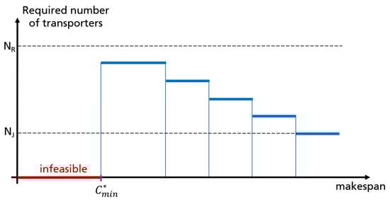
Figure 3.
Minimum number of transporters in an assignment with a given makespan. A feasible solution needs at least one transporter per job. The solution minimizing the makespan does not necessarily require all transporters.
The transporter count in a Pareto optimal solution is as least equal to the number of jobs and at most equal to the transporter count computed by Algorithm .
Our main algorithm in this paper computes, for each transporter count, a solution with the minimum makespan using this number of transporters. This can be done with one binary search per transporter count. At every iteration, we solve an aggregated version of using an MIP solver. Note that when computing a Pareto solution for a given count of every transporter, we choose the transporters with the biggest capacity.
6.2. Heuristics to Compute the Pareto Frontier
Now, we introduce several different heuristic algorithms to approximate the Pareto frontier of a instance.
First, we use simple extensions of the heuristics for the saturated problem to compute the Pareto frontier directly. Then, we show how to achieve alternative heuristics by combining the heuristics for the saturated problem directly with ideas from the first part to approximate solutions of minimum makespan for the general , given a fixed set of transporters. Then, as in the first part, an approximation of the Pareto frontier can be gained by iteratively increasing the number of transporters we are allowed to assign.
6.2.1. Extensions of the Saturated Algorithms
Now, we extend the saturated greedy algorithms , , and to compute a Pareto frontier for . Note that every solution of the Pareto frontier must assign at least one transporter to each job, as otherwise, the makespan is infinite.
It is straightforward to extend the greedy algorithms by transporter and to compute a Pareto frontier, since every iteration already provides a partial assignment using one more transporter. At every iteration, we generate a completed assignment by temporarily providing one transporter to each job that had not received any transporter yet. If we do not have enough transporters to complete the assignment, the algorithm stops and returns the computed Pareto frontier. We denote by and the extension of the greedy heuristics to the general case.
For the greedy algorithm by job , there is no simple way of creating a Pareto frontier. Our extension of algorithm iteratively runs with different transporter counts, always choosing the ones with biggest capacity. For a fixed transporter count, when assigning transporters to a job, must restrict the maximum number of transporters assigned to this job such that the next jobs can still receive at least one transporter. Since Algorithm allows jobs to not be saturated, it becomes more important to order the jobs in a meaningful sequence before assigning the transporters. We sort the jobs by decreasing values of completion time they would have if they were only assigned the smallest transporter. If we denote by the minimum transporter filling time, by Equation (1), that means jobs are sorted by non-increasing value of , depending on the job return time . In our simulations, we will only consider jobs with the same saturated processing time. In this case, our job order is equivalent to ordering the jobs by decreasing return times.
6.2.2. Binary Search Heuristics
In the following, we develop new heuristics by replacing the resolution of program with greedy heuristics in the binary search framework from .
The program consists of minimizing the number of used transporters for a fixed makespan. Hence, Algorithm computes a solution, minimizing the number of used transporters for different makespan values. This is exactly what Algorithm does. Therefore, combining this algorithm with a binary search will not yield any better result.
On the other hand, Algorithms and focus on the idle time per period. The former looks for a combination of transporters saturating a job, while the latter aims at minimizing the maximum idle time per period. In the following, we slightly modify program to look like an instance to and use our greedy algorithms.
The program only differs from a saturated transporter allocation program by the factor in Equation (31). Namely, for every job j:
We rewrite Equations (31) as:
Since the maximum capacity assigned to a job is bounded by the maximum capacity over all transporters , the following constraint is more restrictive:
This more restrictive constraint corresponds to a modified instance of , with a return time of instead of for job j. We call the mixed integer program obtained by replacing Equation (31) with Equations (33), modeling a saturated transporter assignment problem.
We can use this modified framework with any of our greedy heuristics to approximate the Pareto frontier. We denote by and the binary search-based heuristics using Algorithms and respectively to solve .
7. Experiments
In this section, we provide two series of experiments. Firstly, we analyze the computation time and the efficiency of the saturated algorithms, which are the core of our algorithms. Afterward, we take a look at the Pareto frontiers computed for the general problem.
7.1. Simulation Environment
The simulations are done on a ThinkPad T490s with a processor Intel Core i7-8665U with 1.90GHz. Algorithms are implemented under Windows 10 in C#, and we use the open-source library Google-OR-Tools to solve mixed integer programs.
For the sake of simplicity, we restrict our simulations to a limited case study. We evaluate the performance of the algorithms on 100 feasible instances with a limited transporter fleet, using the following scenarios:
- 4 jobs, 20 transporters;
- 5 jobs, 25 transporters;
- 6 jobs, 30 transporters;
- 7 jobs, 35 transporters.
We randomly generate 100 problem instances for each scenario. The number of jobs, number of transporters, as well as the job return times and the transporter filling times are all integers following an uniform distribution. The return time of every job is between 5 and 15, and the filling time of every transporter is between 1 and 5. Therefore, every job will need on average transporters. Every job has the same saturated processing time of 180.
We are interested in three criteria:
- 1
- The average computation time of the algorithm.
- 2
- The number of infeasible instances, where the algorithm did not find an assignment.
- 3
- The number of assigned transporters. Whenever the model is infeasible, we set the number of assigned transporters equal to the total number of transporters. Thus, we choose for this criterion to not penalize infeasible instances compared to a feasible assignment effectively using every transporter at our disposal.
Each of these criteria is sought to be minimized: a good performing algorithm must have low values for these criteria. Note that for saturated algorithms, the completion time of every job is fixed; hence, it does not need to be evaluated.
7.2. Performance of the Saturated Algorithms
We consider the following saturating algorithms:
- Algorithm , assigning transporters to jobs one by one.
- Algorithms and , iteratively assigning transporters to the job with maximum idle time per period and maximum completion time, respectively.
- Algorithm , the mixed integer program grouping transporters with equal filling time.
We excluded the simple mixed integer program , as it turned out that it is already too slow for our problem instances (see Figure 4).
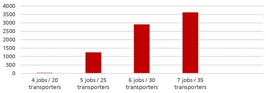
Figure 4.
Average running time of Algorithm over five randomly generated instances, in seconds. We set up the solver with a one hour time-out limit, such that an instance takes a maximum of 3600 s duration.
Figure 5 presents the running times of the algorithms. Algorithm is reasonably fast for our small problem instances of up to 10 jobs. All greedy heuristics always run in a few milliseconds. We remind here that the complexity of Algorithm is exponential in the saturating transporter cardinality, which should not exceed six in our test sets.
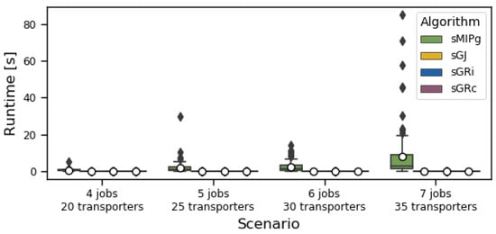
Figure 5.
Distribution of running times of the algorithms, in seconds. The distributions are shown as box plots. The dot shows the average value and the line the median. The box (if it exists) shows the 25% to 75% quantile. If there is no box, then the values in those quantiles coincide with the average. Outliers are shown as diamonds.
Figure 6 and Figure 7 show for every algorithm the total number of infeasible instances and the average number of used transporters, respectively. Since our test sets only contain feasible instances, the optimal algorithm has no infeasible instance. Among the greedy heuristics, the heuristic by job performs better than the heuristics by transporters. This is an intuitive result in saturated scenarios, as looks for the tightest assignment for every job, whereas Algorithms and assign transporters on the fly, without ensuring that the transporters assigned to a same job fit well together. Algorithm , which minimizes the completion time at every step, performs slightly worse than Algorithm , which minimizes the idle time at every step, for a similar reason: since the objective is to remove the idle time, it is more beneficial to focus on the idle time than the completion time, as the latter also depends on the superfluous total size of the job.
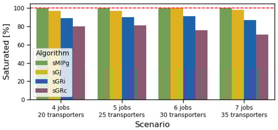
Figure 6.
Share of the 100 instances where the respective algorithms do return a feasible, saturated solution.
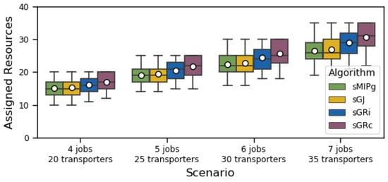
Figure 7.
Distribution of assigned transporters (using the same boxplot settings as in Figure 5). Whenever an instance is infeasible, this number is set to the total number of transporters.
We conclude that when looking for a saturated solution, a good recommendation is to use the greedy heuristic by jobs .
7.3. Performance of the General Algorithms
We now evaluate the Pareto frontier generated by the following algorithms:
- The three greedy algorithms , , and generalizing their saturated counterparts , , and .
- The binary search algorithm solving an aggregated version of by grouping transporters with equal filling time.
- The binary search heuristics and , which are iteratively called respectively and to solve the saturated mixed integer program with altered job return times.
Figure 8 shows the computed Pareto frontiers for our first simulation scenario, using jobs and 20 transporters. Contrary to the saturated case, Algorithm performs poorly for limited transporter fleets, as it over-invests transporters for the first jobs while letting future jobs have a single transporter. Since the last job typically gets assigned the smallest transporter in the fleet, adding an even smaller transporter to the fleet will further increase its completion time, hence potentially increasing the makespan of the assignment. In other words, Algorithm may generate a worse, dominated solution while using a bigger transporter fleet. In order to create a non-increasing Pareto frontier, we set the makespan with N available transporters as the minimum makespan over every instance using at most N transporters.
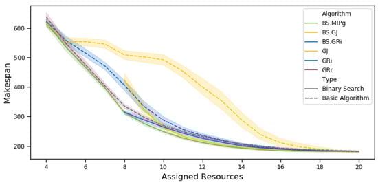
Figure 8.
Median Pareto frontier over 100 instances with 95% confidence intervals. Algorithm computes Pareto optimal solutions, whereas the other algorithms have no optimality guarantee. By design, Algorithms and cannot compute any solution using less than eight transporters.
Algorithm is less efficient than Algorithm for a similar reason: since we want to minimize the maximum job completion time, we should assign more transporters to jobs with the highest residual completion time instead of the job with the highest residual idle time.
However, the binary search-based heuristics generally perform very well when compared to the nearly optimal algorithm , with the exception of when using less than 10 transporters. This shows that virtually increasing the return times of the small jobs (with short saturated processing time) is a good way to balance the transporter fleet between the jobs and ensure a short makespan. Note that the Pareto frontiers generated by the binary search heuristics only start at eight transporters, because each job needs at least two transporters to be saturated.
Finally, Table 2 shows that the binary search-based heuristics are extremely fast, despite being 10 to 100 times slower than their greedy counterpart.
Table 2.
Average running times to compute the Pareto frontiers over 100 instances, in seconds.
We conclude that to solve an instance of the transporter assignment problem, an efficient method consists of iteratively increasing the return time of the jobs until the problem has a saturated solution. Then, the computed saturated solution is a good solution to the initial assignment problem. An advantage of this method is that the saturated problem instances do not have to be solved to optimality, and most decent algorithms should induce a good solution to the transporter assignment problem.
8. Conclusions
The objective of the transporter allocation problem is to assign transporters to jobs to jointly minimize the makespan of the jobs and the number of assigned transporters. Crucially, transporters have a limited capacity, and usually, multiple transporters are assigned to a single job. After processing a share of the job load, a transporter must wait for a given time before it can process the job again. In particular, the goal is to compute the frontier of Pareto optimal solutions.
To the best of our knowledge, this is the first study on the assignment of an heterogeneous transporter fleet where transporters are regarded as a dynamic resource impacting the completion times and not as a fixed requirement.
We show that in general, it is NP-hard in the strong sense to compute even a single point on the Pareto frontier. In particular, it is NP-complete to decide whether a solution exists where every job has the same minimum completion time. Furthermore, the problem remains NP-hard in the usual sense, even if there are only two jobs.
On the other hand, when every transporter is identical, the whole Pareto frontier can be computed in a runtime polynomial in the number of jobs and transporters.
We provide several exact algorithms and heuristics to compute the minimum number of transporters needed such that all jobs are contracted to their minimum completion time. Then, we use these results to compute Pareto frontiers for general instances, both exactly and heuristically. Computational experiments show that our heuristics compute quickly decent approximations of the optimal solution, where the mixed integer program is already slow.
The results presented in this paper are part of a wider, practical study, in which we used a multi-level approach to solve applied problems in farming logistics together with an industrial partner. Assigning transporters to jobs was one of several levels of decision making in this regard, and our algorithms (adjusted for some additional practical needs) have proven to be useful also in early applied experiments.
In this paper, we assumed that every team of transporters only completes a single job. However, depending on the job sizes, there are also a variety of practical applications, where transporters are grouped into teams to fulfill several jobs per day in a sequence. Removing this limitation in a future study would significantly increase the number of use cases to which our results can be applied. Note that moving from one job to another may induce location-dependent traveling times, which we did not need to take into account in this paper. Even though we expect a single move from one job (or from the hub) to the next job to only have a minor impact on the solution, it will be important to find the best time to switch a transporter from one job to the next. Another challenge would be how to decide which jobs should be served by the same transporter team and which should receive a different team. Such a clustering, if not mandated by practical circumstances such as large travel times between the jobs, would be an additional degree of freedom, which can have a large impact on the optimality of a solution.
As a further area of extension, note that in our model, it is implicitly assumed that all teams of transporters are disjointed (since each transporter can only be assigned to one job). This is common practice to simplify the planning task, but it can lead to less efficient solutions. In some applications, such as [2,4], transporters are allowed to alternate between different jobs, optimizing the usage of each machine and hence providing better solutions. Allowing this for our problem would add an additional layer of difficulty. In particular, period lengths would no longer be constant but would differ, depending on when some transporters may serve another job. The scheduling decision, when to switch transporters to another job, would be much more impactful, and the scheduling of transporters to process each job would most likely have to be dealt with explicitly in that case.
Author Contributions
Conceptualization, N.L. and N.J.; methodology, N.J., N.L. and C.W.; software, N.J.; validation, N.J.; formal analysis, N.J., N.L. and C.W.; investigation, N.J., N.L. and C.W.; resources, N.J.; data curation, N.J. and N.L.; writing—original draft preparation, N.J. and N.L.; writing—review and editing, N.J., N.L. and C.W.; visualization, N.J. and N.L.; supervision, N.L.; project administration, N.L.; funding acquisition, N.L. All authors have read and agreed to the published version of the manuscript.
Funding
This research received no external funding.
Institutional Review Board Statement
Not applicable.
Informed Consent Statement
Not applicable.
Data Availability Statement
The input data of our numerical experiments presented in this study are openly available in Zenodo at https://zenodo.org/record/5583977#.YgYc79_MKUk (accessed 11 February 2022).
Acknowledgments
We thank Sven Krumke from TU Kaiserslautern for his helpful ideas concerning the NP-hardness proof (Theorem 1). We also thank our colleagues Sebastian Velten and Sven Jäger for helpful discussions and suggestions.
Conflicts of Interest
The authors declare no conflict of interest.
Abbreviations
The following abbreviations are used in this manuscript:
| Transporter Assignment Problem | |
| Decision version of the Transporter Assignment Problem | |
| Saturated Transporter Assignment Problem | |
| Complexity order of the algorithm | |
| (Hom) | Our algorithm for with homogeneous transporters |
| Heuristic for , greedily assigning a transporter to the job with maximum | |
| idle time per period | |
| Heuristic for , greedily assigning a transporter to the job with maximum | |
| makespan | |
| Heuristic for , greedily generating an saturating assignment to each job | |
| Extension of to compute a Pareto frontier for | |
| Extension of to compute a Pareto frontier for | |
| Extension of to compute a Pareto frontier for | |
| MIP | Mixed Integer Program |
| MIP formulation of | |
| MIP formulation of aggregating transporters by model | |
| MIP formulation of with fixed job idle rates | |
| MIP formulation of with fixed job idle rates and altered job return times | |
| Algorithm framework to compute a solution of with minimum makespan | |
| Exact algorithm for , using framework and an MIP solver for | |
| Heuristic for , using framework and to generate a solution | |
| for | |
| Heuristic for , using framework and to generate a solution | |
| for | |
| Set of jobs | |
| Set of transporters | |
| Set of transporter models | |
| Number of jobs | |
| Number of transporters | |
| Number of transporter models | |
| Number of transporters with model m | |
| j | Job variable |
| r | Transporter variable |
| m | Transporter model variable |
| Filling time of transporter r | |
| Return time of job j | |
| Saturating transporter cardinality for job j | |
| Boolean value of “transporter r is assigned to Job j” | |
| Number of transporters assigned to Job j | |
| Number of “transporters with model m assigned to Job j” | |
| Boolean value of “At least one transporter with model m is assigned to Job j” | |
| Completion time of job j given assignment | |
| Makespan given assignment = maximum job completion time | |
| Minimum makespan over all feasible solutions | |
| Saturated processing time of job j | |
| Makespan in a saturated solution = maximum saturated job processing time | |
| Idle time per period for job j | |
| idle rate per period for job j to have completion time C | |
| Period length for job j |
Appendix A. Proof of the Completion Time Estimate Given by Equation (1)
In this appendix, we show that the completion time estimate as given in Section 1, Equations (1)–(3) is accurate. To be precise, our goal is to show the following theorem.
Theorem A1.
Since in our practical applications, usually and therefore also is much larger than the return time , Theorem A1 implies that the error incurred by using Equation (1) to estimate the completion times of jobs is negligible.
For the remainder of this appendix, we use notations R, j, , , and as defined in Theorem A1. Furthermore, we continue to denote by the estimated completion time of job j as given by Equation (1). Finally, let the resources in R be given as , as numbered by the non-increasing order of filling times.
We first proof the following Lemma.
Lemma A1.
If
then, the transporters in R saturate job j, i.e., .
Proof.
Note that if then by definition of . In particular, for any subset with exactly elements, it holds that This means that using the transporters in R in a cyclic fashion, a transporter always returns before all other transporters finish their processing of job j. Thus, job j can be processed without idle times and the transporters in R saturate job j. □
Consider next the schedule in which transporters in R are used in a cyclic fashion, in order of their numbering, that is, they use each transporter once, in order of the transporter numbering, then restart with transporter and continue, again in order of the transporter numbering and so on, until job j is fully finished. Denote this schedule by and its completion time by .
Lemma A2.
- 1
- In schedule , the time between the starts of two uses of transporter is exactly .
- 2
- In schedule , between any two uses of transporter , job j is idle for exactly time. Furthermore, all idle time, if any, appears immediately before the second use of .
- 3
- It holds that
Proof.
Proof of 1: By Lemma A1, if , then job j is saturated and clearly the time between the starts of two uses of a transporter r is given as the sum of filling times of all transporters, which is exactly . On the other hand, is a lower bound for the time between the starts of two uses of any transporter, since between two starts, the transporter needs to finish its processing and then its whole return time. Since from , it follows that , this means by the time returns, no other transporter is processing job j so it can start immediately, leading again to a time of between any two starts of uses of .
Proof of 2: Since, by definition, if and only if and by Lemma A1 this means job j is saturated, in that case, the statement holds. Suppose and . In that case, since during time , each transporter processes job j exactly once, by construction of schedule , the total time spent idle is given as
by definition. Finally, note that due to the ordering of jobs in , the time between the start of a use of any transporter r and the next time r is needed is given by , so any transporter other than always arrives back at site before it is needed again. Therefore, any idle time can only happen before a use of transporter .
Proof of 3: During any time , exactly time is spent processing in schedule , by Statement 1 and 2 of this Lemma. Thus, after time,
of job j has been processed. It remains an amount of either exactly if divides or , otherwise, which combined yields a remaining amount of
Finally, note that the remaining amount can be processed immediately and without interruption, since after time , transporter is ready to process, and by the second statement of this lemma, no further idle time happens before all the remaining amount is processed. □
Obviously, it holds that . Furthermore, note that
where the last inequality is due to . Therefore, it is proven that .
We are left to prove that . First, we show the following lemma, extending the statement of Lemma A2 (2).
Lemma A3.
In any schedule using transporters in R to process job j, between two uses of transporter , idle time of at least happens.
Proof.
If , there is nothing to prove. So assume and . In the proof of Lemma A2, it was shown that if every other transporter is used exactly once between two uses of , then between the two uses of , the idle time of exactly is reached. Using fewer transporters in between does obviously not reduce idle time. On the other hand, using any other transporter twice without using in between leads to an idle time between the two uses of of at least
which means the idle time between the two uses of would also be larger, which finishes the proof. □
Using Lemma A3 and Equation (A1), we can prove the following lemma.
Lemma A4.
For any schedule using transporters in R to process job j, let transporter be a transporter with the most uses and let be used exactly ℓ times. Then, job j is idle for at least
time.
Proof.
If is used ℓ times, by Lemma A3, job j is idle for at least , and the statement is proven. So, assume transporter is used times. By Lemma A3, between any two uses of transporter , idle time of at least appears. However, by Equation (A1), between any two uses of job where is not used in between, idle time of at least
appears. Thus, the total idle time of job j is at least
time units long. □
Note that using schedule , each transporter can be used ℓ times, causing idle time of at most . Thus, by Lemma A4, we have
Furthermore,
Therefore, and due to Equation A2, we have , which finishes the proof of Theorem A1. Note that in the case where the transporters in R saturate job j and , then the above and Equation A2 even imply that . In addition, note that we actually showed that , and thus the worst case estimate as given in Theorem A1 can only happen when only a single transporter is assigned to a job (which is the only time when ).
References
- Jensen, M.F.; Bochtis, D.; Sørensen, C.G. Coverage planning for capacitated field operations, part II: Optimisation. Biosyst. Eng. 2015, 139, 149–164. [Google Scholar] [CrossRef]
- Aliano Filho, A.; Melo, T.; Pato, M.V. A bi-objective mathematical model for integrated planning of sugarcane harvesting and transport operations. Comput. Oper. Res. 2021, 134, 105419. [Google Scholar] [CrossRef]
- Kuenzel, R.; Teizer, J.; Mueller, M.; Blickle, A. SmartSite: Intelligent and autonomous environments, machinery, and processes to realize smart road construction projects. Autom. Constr. 2016, 71, 21–33. [Google Scholar] [CrossRef]
- Payr, F.; Schmid, V. Optimizing deliveries of ready-mixed concrete. In Proceedings of the 2009 2nd International Symposium on Logistics and Industrial Informatics, Linz, Austria, 10–12 September 2009; pp. 1–6. [Google Scholar]
- Wörz, S.K. Entwicklung Eines Planungssytems zur Optimierung von Agrarlogistik-Prozessen. Ph.D. Thesis, Technische Universität München, Munich, Germany, 2017. [Google Scholar]
- Lopez Milan, E.; Miquel Fernandez, S.; Pla Aragones, L.M. Sugar cane transportation in Cuba, a case study. Eur. J. Oper. Res. 2006, 174, 374–386. [Google Scholar] [CrossRef]
- Salassi, M.E.; Barker, F.G. Reducing harvest costs through coordinated sugarcane harvest and transport operations in Louisiana. J. Am. Soc. Sugar Cane Technol. 2008, 28, 32–41. [Google Scholar]
- Ahmadi-Javid, A.; Hooshangi-Tabrizi, P. Integrating employee timetabling with scheduling of machines and transporters in a job-shop environment: A mathematical formulation and an Anarchic Society Optimization algorithm. Comput. Oper. Res. 2017, 84, 73–91. [Google Scholar] [CrossRef]
- Bochtis, D.D.; Sørensen, C.G.; Busato, P. Advances in agricultural machinery management: A review. Biosyst. Eng. 2014, 126, 69–81. [Google Scholar] [CrossRef]
- Kusumastuti, R.D.; van Donk, D.P.; Teunter, R. Crop-related harvesting and processing planning: A review. Int. J. Prod. Econ. 2016, 174, 76–92. [Google Scholar] [CrossRef]
- Garey, M.R.; Johnson, D.S. Computers and Intractability; Freeman: San Francisco, CA, USA, 1979; Volume 174. [Google Scholar]
- Morales-Chávez, M.M.; Soto-Mejía, J.A.; Sarache, W. A mixed-integer linear programming model for harvesting, loading and transporting sugarcane: A case study in Peru. DYNA 2016, 83, 173–179. [Google Scholar] [CrossRef]
- Ehrgott, M. Multicriteria Optimization; Springer Science & Business Media: Berlin/Heidelberg, Germany, 2005; Volume 491. [Google Scholar]
- Ralphs, T.K.; Kopman, L.; Pulleyblank, W.R.; Trotter, L.E. On the capacitated vehicle routing problem. Math. Program. 2003, 94, 343–359. [Google Scholar] [CrossRef]
- Bharadwaj, V.; Ghose, D.; Robertazzi, T.G. Divisible load theory: A new paradigm for load scheduling in distributed systems. Clust. Comput. 2003, 6, 7–17. [Google Scholar] [CrossRef]
- Ghanbari, S.; Othman, M. Comprehensive Review on Divisible Load Theory: Concepts, Strategies, and Approaches. Math. Probl. Eng. 2014, 2014, 1–13. [Google Scholar] [CrossRef]
- Drozdowski, M.; Lawenda, M. The combinatorics in divisible load scheduling. Found. Comput. Decis. Sci. 2005, 30, 297–308. [Google Scholar]
- Shakhlevich, N.V. Scheduling Divisible Loads to Optimize the Computation Time and Cost. In Economics of Grids, Clouds, Systems, and Services; Altmann, J., Vanmechelen, K., Rana, O.F., Eds.; Springer International Publishing: Cham, Switzerland, 2013; pp. 138–148. [Google Scholar]
- Drozdowski, M.; Shakhlevich, N. Scheduling divisible loads with time and cost constraints. J. Sched. 2019, 24, 507–521. [Google Scholar] [CrossRef]
- Salkin, H.M.; De Kluyver, C.A. The knapsack problem: A survey. Nav. Res. Logist. Q. 1975, 22, 127–144. [Google Scholar] [CrossRef]
- Hiley, A.; Julstrom, B.A. The quadratic multiple knapsack problem and three heuristic approaches to it. In Proceedings of the 8th Annual Conference on Genetic and Evolutionary Computation, Seattle, WA, USA, 8–12 July 2006; pp. 547–552. [Google Scholar]
- Boyer, V.; Elkihel, M.; El Baz, D. Heuristics for the 0–1 multidimensional knapsack problem. Eur. J. Oper. Res. 2009, 199, 658–664. [Google Scholar] [CrossRef]
- Chekuri, C.; Khanna, S. A polynomial time approximation scheme for the multiple knapsack problem. SIAM J. Comput. 2005, 35, 713–728. [Google Scholar] [CrossRef]
- Jansen, K. Parameterized Approximation Scheme for the Multiple Knapsack Problem. SIAM J. Comput. 2010, 39, 1392–1412. [Google Scholar] [CrossRef]
- Martello, S.; Toth, P. A Bound and Bound algorithm for the zero-one multiple knapsack problem. Discret. Appl. Math. 1981, 3, 275–288. [Google Scholar] [CrossRef]
- Pisinger, D. An exact algorithm for large multiple knapsack problems. Eur. J. Oper. Res. 1999, 114, 528–541. [Google Scholar] [CrossRef]
- Dawande, M.; Kalagnanam, J.; Keskinocak, P.; Salman, F.S.; Ravi, R. Approximation algorithms for the multiple knapsack problem with assignment restrictions. J. Comb. Optim. 2000, 4, 171–186. [Google Scholar] [CrossRef]
- Brauner, N.; Crama, Y.; Grigoriev, A.; van de Klundert, J. A Framework for the Complexity of High-Multiplicity Scheduling Problems. J. Comb. Optim. 2005, 9, 313–323. [Google Scholar] [CrossRef][Green Version]
Publisher’s Note: MDPI stays neutral with regard to jurisdictional claims in published maps and institutional affiliations. |
© 2022 by the authors. Licensee MDPI, Basel, Switzerland. This article is an open access article distributed under the terms and conditions of the Creative Commons Attribution (CC BY) license (https://creativecommons.org/licenses/by/4.0/).