Intensity and Direction of Volatility Spillover Effect in Carbon–Energy Markets: A Regime-Switching Approach

Abstract

This paper advances a volatility-regime-switching mechanism to investigate the intensity and direction of the volatility spillover effect in carbon–energy markets. Switching between a low-volatility (LV) and high-volatility (HV) regime, our mechanism involves a four-state system (i.e., LV-LV, HV-LV, LV-HV and HV-HV). Our findings are listed as follows: First, the highest EUA–WTI correlation occurs when both are in an HV regime (i.e., HV-HV), revealing the intensity of the volatility spillover effect. Second, when EUA and WTI are experiencing an opposite volatility regime (one in LV and the other in HV), a higher EUA–WTI correlation is observed when WTI is in an HV regime. This result implies that the direction of the volatility spillover effect is from the energy market to the carbon market. Third, the regime-switching model involving the non-uniform volatility–correlation relations outperforms the conventional GARCH and DCC models in volatility forecasting and portfolio construction.

1. Introduction

Carbon markets have attracted attention following concerns around climate change [1]. Thanks to the European Union Emissions Trading System, established in 2005, carbon assets have become an available investment option for investors. Firms, particularly firms with high energy consumption, are also concerned about carbon markets since their costs rely on carbon and energy prices. For policymakers, carbon markets provide them with information to form appropriate policies to manage carbon emissions and energy consumption.

The literature has examined the connectedness between carbon and energy markets and has offered evidence of their correlations (see [2] for a summary). This study contributes to the carbon–energy literature in three ways. First, we develop a theoretical perspective on the volatility–correlation relationships in carbon–energy markets to break down the fundamental channel and the volatility spillover effect, two significant factors causing the link between the two markets. The fundamental channel is based on real and economic ties between the two markets. Economic growth stimulates energy consumption and, thus, produces carbon emissions. Given this common factor (i.e., economic growth), the correlation between carbon and energy markets is straightforward. Beyond the fundamental channel, this study highlights the volatility spillover effect and presumes that this effect increases the carbon–energy correlation. Moreover, we re-examine the direction of the volatility spillover effect in carbon–energy markets using a regime-switching approach. In brief, if the carbon–energy correlation grows due to a high volatility condition of the energy market; volatility spillover is from the energy market to the carbon market. By contrast, if a high carbon–energy correlation is observed when the carbon market faces a high-volatility condition, the volatility spillover direction is from the carbon market to the energy market. To date, the existing carbon–energy market literature has not considered these dynamic volatility–correlation relationships. In this study, we address these relationships and use them to re-examine the intensity and direction of the volatility spillover effect in carbon–energy markets.

Second, to examine the dynamic volatilities and correlations in carbon–energy markets, most studies [3,4,5] adopt the conventional time-dependent approaches, including the GARCH (Generalized Autoregressive Conditional Heteroskedasticity) and DCC (Dynamic Conditional Correlations) models. While the GARCH and DCC models are the most popular methodologies used for market volatilities and correlations, they suffer from some limitations. First, the GARCH-based volatilities cannot control discrete volatility jumps in markets [6,7]. Second, prior studies use a two-step estimation method for the DCC models, which implicitly assumes independence between volatilities and correlations (see Section 2.2). This study employs a regime-switching approach to identify volatility state combinations in carbon–energy markets and jointly analyzes their correlation dynamics. Our one-step estimation method mitigates the sample selection bias due to a two-step estimation process [8].

Third, we conduct two practical tests: volatility forecasting and portfolio construction, to offer evidence to support the use of our regime-switching approach against the conventional time-varying approaches, including the GARCH and DCC models. Our empirical results show that carbon–energy correlations significantly diverge across various volatility state groupings. Accordingly, this study conducts two practical tests: portfolio risk forecasting and portfolio construction. We argue that volatilities and correlations are the two critical elements for risk management; thus, the consideration of volatility–correlation relationships may enhance the performance of the tasks. To the best of our knowledge, prior studies have not conducted these two practical tests on carbon–energy market data.

We proceed with the study as follows: First, in Section 2, we review related studies and then develop our research questions. Next, we introduce the models used in this study, including the conventional GARCH and DCC models and our proposed regime-switching model, in Section 3. In addition, we explain why our proposed regime-switching approach is more appropriate than the traditional GARCH and DCC models in detecting the intensity and direction of the volatility spillover effect in carbon–energy markets. In Section 4, we report the estimation results. Next, Section 5 discusses the results and conducts the two practical tests: volatility forecasting and portfolio construction. Finally, we conclude the paper in Section 6.

2. Literature Review and Research Question Development

2.1. Studies on Carbon–Energy Correlations

Climate change issues are triggering research interest in carbon–energy correlations in the past decade [9]. Carbon–energy correlations are critical for investors, energy-intensive industries, and policymakers. The literature has offered significant evidence of carbon–energy correlations. For example, Chevallier [10] demonstrates that economic activities (proxied by industrial productions) and energy prices may drive carbon prices. Tan and Wang [11] show the impact of energy prices and macroeconomic risk factors (proxied by a stock market index, the commodity price, and US Treasury bill yield) on carbon. Zhao et al. [12] investigate the relationship between energy prices and carbon prices and indicate that one may use energy prices to predict carbon prices. Lin and Jia [13] examine the impact of the carbon price on economic outputs and suggest that the effect is more pronounced in energy industries than in other industries.

In addition to testing the carbon–energy correlations based on the return spillover effect (i.e., the first moment), a few recent studies have turned their attention to the volatility spillover effect (i.e., the second moment). Notably, most of these studies employ the conventional GARCH and DCC models to examine this effect [14,15,16,17,18,19] (some researchers develop other methodologies to address the volatility spillover effect. For instance, Wang and Guo [20] and Tan et al. [9] follow Diebold and Yilmaz [21] to construct the spillover index for carbon–energy markets. Ji et al. [22] employ the VAR model to test the effect.). While these prior studies have documented the volatility spillover effect in carbon–energy markets, we argue that the conventional GARCH and DCC models have certain shortcomings. First, the GARCH-based models fail to control for structural changes in volatility (i.e., volatility jumps) and, thus, encounter the high-persistence issue in volatility estimation and low accuracy in volatility prediction [23,24]. Second, with regard to the DCC models, prior empirical studies invariably employ a two-step approach to estimate the model parameters. Specifically, in the first step, they estimate the univariate GARCH model for each asset (e.g., carbon and energy assets in this study). After calculating the residual of the univariate asset, they estimate the DCC models in the second step. This two-step approach implicitly assumes that volatility estimation is irrelevant to correlation estimation and, thus, cannot address their relationships [25]. Therefore, this study uses a regime-switching approach to address the volatility–correlation relationships and adopts a one-step estimation approach (see Section 3.1). Moreover, we use the proposed volatility–correlation relationships to develop a theoretical hypothesis regarding the intensity and direction of the volatility spillover effect in carbon–energy markets (see the subsequent subsection).

2.2. Research Question Development

Our research aims to contribute to the carbon–energy correlation literature. We develop combinations of market volatility states in carbon–energy markets and differentiate two cross-market channels: fundamental and volatility spillover. Further, we use our proposed dynamic volatility–correlation relationships to examine the intensity and direction of the volatility spillover effect in carbon–energy markets. Our conjectures are explained as follows: First, as defined in the literature, the fundamental channel is based on real and economic links between the paired markets. Researchers point out three effects: aggregated demand effect, substitution effect, and production restrain effect, supporting the fundamental link. Beyond the fundamental channel, recent studies turn their attention to the volatility spillover effect in carbon–energy markets. Two models may explain the volatility spillover effect. The first model is the cross-market rebalancing model proposed by Kodres and Pritsker [26]. They hypothesize that cross-market shocks occur because investors optimally adjust their investment in one market to respond to shocks in another market. The second model is the social learning model proposed by Trevino [27]. He hypothesizes that cross-market contagions occur because investors fear a crisis in one market after observing a crisis in the other market.

This study addresses two derivative questions regarding the two cross-market channels. The first question is how does one distinguish the impacts of the two channels (i.e., fundamental and volatility spillover) on carbon–energy correlations? The second question is how does one detect the direction of the volatility spillover channel in carbon–energy markets? We argue that the key to answering the two questions is carbon–energy market volatility conditions. Below, we list our conjectures. First, financial crises go along with high market volatility [28,29,30,31]. Accordingly, we argue that the volatility spillover effect will be maximal when carbon–energy markets encounter a high-volatility condition. Moreover, considering the difference between a low-volatility (LV) and a high-volatility (HV) regime for each market, we may develop a four-volatility-state system for carbon–energy markets: i.e., LV-LV, HV-LV, LV-HV, and HV-HV.

Next, we conduct two comparative analyses to answer our two research questions on carbon–energy correlation dynamics. The first comparative analysis is based on the LV-LV versus HV-HV state. The HV-HV state reflects extreme economic and/or financial distresses, causing both carbon and energy markets to experience volatile price movements (4.5% of our test sample, see Table 6). By contrast, the LV-LV state presents the situation when both carbon and energy markets live in a common and non-volatile state (64.54% of our test sample, see Table 6). We argue that the impact of the volatility spillover effect on carbon–energy correlations primarily shows up in the HV-HV state. On the other hand, under the LV-LV state, the carbon–energy correlations are mainly driven by the fundamental channel. Accordingly, the comparative analysis between the LV-LV and HV-HV states may offer a test on the intensity of the volatility spillover effect.

To examine the direction of the volatility spillover (the second research question in our study), we conduct a comparative analysis between the other two states: HV-LV versus LV-HV. These two volatility states reflect that only one market (carbon or energy) is experiencing an HV condition. If carbon–energy correlations stimulate when the energy market is under an HV state, it shows that the volatility spillover direction is from the energy market to the carbon market. On the other hand, if we observe a higher carbon–energy correlation when the carbon market faces an HV state, the result implies that the volatility spillover path is from the carbon market to the energy market. The subsequent subsection uses the regime-switching model to identify a low-volatility (LV) and a high-volatility (HV) regime for each carbon and energy market. Next, we develop a four-volatility-state system for the non-uniform volatility–correlation relationships. Finally, we employ these relationships to re-examine the intensity and direction of the volatility spillover channel in carbon–energy markets. It should be noted that we adopt a one-step estimation process to determine all the volatility and correlation parameters in the models.

3. Research Models

Prior studies commonly use GARCH models to examine dynamic conditional variances and DCC models to examine dynamic conditional correlations. Nonetheless, the pure time-varying process involved in these models cannot identify nonlinear volatility jumps and state-dependent correlations [32,33]. In this section, we propose a regime-switching approach to handle these nonlinearities and test our hypotheses regarding the intensity and direction of the volatility spillover effect. For comparative analysis purposes, we start this section by first introducing the conventional time-varying approaches (i.e., GARCH and DCC) as a benchmark against our proposed regime-switching approach.

3.1. Bivariate GARCH Model

The bivariate GARCH model commonly used in the existing studies on the research of carbon–energy markets is presented below:

$$r_t^{EUA}={\mu }^{EUA}+{\phi }^{EUA}·r_{t-1}^{EUA}+e_t^{EUA}$$

(1)

$$r_t^{WTI}={\mu }^{WTI}+{\phi }^{WTI}·r_{t-1}^{WTI}+e_t^{WTI}$$

(2)

$$e_t|{\mathsf{\Phi }}_{t-1}=\left[\begin{array}{c}{e}_t^{EUA}\\ e_t^{WTI}\end{array}\right] ~ BN \left(0, H_t\right)$$

(3)

$$H_t=\left[\begin{array}{cc}{h}_t^{EUA}& h_t^{EUA,WTI}\\ h_t^{EUA,WTI}& h_t^{WTI}\end{array}\right]$$

(4)

where $r_t^{EUA}$ and $r_t^{WTI}$, respectively, represent the daily returns on EUA (carbon market) and WTI (energy market) observed on day t. Since our focus is on the second moment (i.e., variances and correlations), we adopt a relatively straightforward first-order autoregressive process for our mean equations, i.e., Equations (1) and (2).

Next, we intoduce the equations for the second moment. As depicted in Equation (3), the residual returns, $e_t^{EUA}$ and $e_t^{WTI}$, follow a bivariate normal distribution (BN). The elements of the conditional variance–covariance matrix (H_t) follow the standard time-varying GARCH specifications:

$$h_t^{EUA}={\omega }^{EUA}+{\alpha }^{EUA}·{(e_{t-1}^{EUA})}^2+{\beta }^{EUA}·h_{t-1}^{EUA}$$

(5)

$$h_t^{WTI}={\omega }^{WTI}+{\alpha }^{WTI}·{(e_{t-1}^{WTI})}^2+{\beta }^{WTI}·h_{t-1}^{WTI}$$

(6)

$$h_t^{EUA, WTI}=\rho \times {\left(h_t^{EUA}·h_t^{WTI}\right)}^{1/2}$$

(7)

where $h_t^{EUA}$ and $h_t^{WTI}$ represent the time-varying conditional variances of EUA (energy market) and WTI (energy market) returns, respectively, and $h_t^{EUA, WTI}$ is the time-varying conditional covariance of the two returns.

3.2. DCC Model

To capture the dynamic conditional EUA–WTI correlation, the existing studies mainly follow Engle [34] to use the DCC model as follows:

$$h_t^{EUA, WTI}={\rho }_t\times {\left(h_t^{EUA}·h_t^{WTI}\right)}^{\frac{1}{2}}$$

(8)

$${\rho }_t=q_t / \sqrt{1+q_t^2}$$

(9)

where

$$q_t=\tau +\pi ·q_{t-1}+\lambda ·e_{t-1}^{EUA}·e_{t-1}^{ETI}/\sqrt{h_{t-1}^{EUA}·h_{t-1}^{ETI}}$$

(10)

Equation (10) depicts the adopted DCC model consisting of three components: (1) the constant unconditional correlation (τ), (2) the lagged conditional correlation as a linear function of q_t−1, and (3) the cross-product term of the lagged standardized residuals. With the transformation function represented by Equation (9), we ensure that the conditional correlation ρ_t lies between −1 and 1. In particular, ρ_t has the same sign as q_t. The larger the magnitude of q_t, the closer ρ_t approaches 1 or −1. It is worth noting that the CCC (constant conditional correlation) model is a special case of the DCC model under the restriction of π = λ = 0 in Equation (10).

3.3. Bivariate SWARCH Model

The GARCH (see Equations (5) and (6)) and DCC models (see Equations (9) and (10)) accommodate the variance- and correlation-clustering behaviors, respectively (the persistence of variance/correlation over time), which are commonly observed in the financial markets. This study proposes a regime-switching approach to investigate our hypothesis of intensity and direction of volatility spillover effect in carbon–energy markets (see Section 2.2). In particular, we extend Hamilton and Susmel’s (1994) Markov-switching Autoregressive Conditional Heteroskedasticity (SWARCH) model to investigate the regime-switching pattern for market volatility (i.e., switching between a low- and high-volatility regime) and the regime-switching volatility–correlation relations. Considering the two asset positions in the carbon–energy portfolio, we develop a bivariate SWARCH model as follows:

$$h_t^{EUA}=g_{s_t^{EUA}}^{EUA}\times \left[{\omega }^{EUA}+{\alpha }^{EUA}·{(e_{t-1}^{EUA})}^2/g_{s_{t-1}^{EUA}}^{EUA}\right]$$

(11)

$$h_t^{WTI}=g_{s_t^{WTI}}^{WTI}\times \left[{\omega }^{WTI}+{\alpha }^{WTI}·{(e_{t-1}^{WTI})}^2/g_{s_{t-1}^{WTI}}^{WTI}\right]$$

(12)

We explain the state-dependent nature involved in Equations (11) and (12) as follows: First, the state variables, s_t^EUA and s_t^WTI, have two possible outcomes: 1 or 2. Second, under Regime I (i.e., the state variable = 1), the conditional variance of EUA is g₁^EUA times ARCH (1) process, and the conditional variance of WTI is g₁^WTI times ARCH (1) process. Under Regime II, (i.e., the state variable = 2), the conditional variance of EUA is g₂^EUA times ARCH (1) process, and the conditional variance of WTI is g₂^WTI times ARCH (1) process (some researchers [35,36,37,38] propose the use of the Markov-switching GARCH (MS-GARCH) model to handle regime-switching conditional variance. However, the MS-GARCH model suffers from an ad hoc assumption in merging the state-dependent conditional variances into a single value that does not depend on the regime path. Augustyniak [39] employs certain simulation methods to show that the estimates obtained from this collapsing procedure are biased and inconsistent. In the present study, we attempt to extend our empirical analysis by using a bivariate MS-GARCH model to capture the dynamic variance/correlation structure of stock and cryptocurrency returns. However, we cannot obtain valid estimation results since the Hessian matrix is singular and, thus, cannot be inverted. While the literature suggests that the MS-GARCH model offers an efficient way to model regime-switching conditional variance, it is not practical to apply a bivariate version of it to model conditional correlation given the technical problems as mentioned above. As such, in our empirical analysis, we adopt the bivariate SWARCH model, which is found to be robust in capturing regime-switching conditional correlations through their relationships with conditional variances). Third, Without loss of generality, we follow Ramchand and Susmel [40] to normalize g₁^EUA = g₁^WTI = 1. Therefore, the conditional variances under Regime II are g₂^EUA and g₂^WTI times the variances under Regime I for EUA and WTI returns. Last, based on our subsequent empirical analysis (presented in Section 4), the estimated g₂^EUA and g₂^WTI coefficients are significantly larger than unity. Accordingly, we define Regime I as the low-volatility (LV) regime and Regime II as the high-volatility (HV) regime.

Given the two separate volatility regimes for EUA and WTI, we generate four different possible states of the EUA–WTI market: (1) s_t^EUA = 1 and s_t^WTI = 1, (2) s_t^EUA = 1 and s_t^WTI = 2, (3) s_t^EUA = 2 and s_t^WTI = 1, and (4) s_t^EUA = 2 and s_t^WTI = 2. Next, we develop the conditional covariance between the EUA and WTI returns as follows:

$$h_t^{EUA, WTI}={\rho }_{s_t^{EUA},s_t^{WTI}}\times {\left(h_t^{EUA}·h_t^{WTI}\right)}^{1/2}$$

(13)

According to Equation (12), when both the carbon and the energy markets are in their LV state (i.e., s_t^EUA = 1 and s_t^WTI = 1), the conditional correlation is ρ_1,1. When both markets are in their HV state (i.e., s_t^EUA = 2 and s_t^WTI = 2), the correlation becomes ρ_2,2. When the two markets are in opposite volatility states (i.e., one market in the HV state while the other in the LV state), the correlation is ρ_1,2. (when s_t^EUA = 1 and s_t^WTI = 2) or ρ_2,1. (when s_t^EUA = 2 and s_t^WTI = 1). Our four-state conditional covariance framework can be considered as a generalized version of that of Edwards and Susmel [41], where a two-state correlation is defined by the two regimes of a single asset.

Finally, to model the switching between the two states separately for each of the two markets, we adopt a first-order Markov chain process, and its transition probabilities are specified as:

$$P\left(s_t^{EUA}=1|s_{t-1}^{EUA}=1\right)=p_{11}^{EUA}, P\left(s_t^{EUA}=2|s_{t-1}^{EUA}=2\right)=p_{22}^{EUA}$$

(14)

$$P\left(s_t^{WTI}=1|s_{t-1}^{WTI}=1\right)=p_{11}^{WTI}, P\left(s_t^{WTI}=2|s_{t-1}^{WTI}=2\right)=p_{22}^{WTI}$$

(15)

where $p_{11}^{EUA}$ is the probability for the carbon market to remain in Regime I from time t − 1 to time t, whereas $p_{22}^{EUA}$ is the probability to remain in Regime II. A similar definition is applied to the energy market.

4. Data and Estimation Results

4.1. Data

This study employs the EUA (European Union Allowances) spot price for the carbon price and the WTI (West Texas Intermediate) crude oil spot price for the energy market price. Next, we empirically use the data to test the non-uniform volatility–correlation relationships in carbon–energy markets. The testing period is between 16 March 2009 and 24 November 2021, consisting of 3311 daily observations (the WTI oil price on 20 April 2021 is negative, which causes the return rates (logarithmic change) on the 20th and 21st of April 2021 to be incalculable. Thus, we exclude the two days in our analysis). The data source is DATASTREAM.

Table 1. Basic statistics of EUA and WTI.

	EUA	WTI
Panel A: Natural log level
Mean	2.4113	4.1823
Q1	1.8213	3.9300
Median (Q2)	2.9143	4.4894
Q3	2.3116	4.2015
S.D.	0.7081	0.3417
Skewness	0.4987	−0.6036
Kurtosis	2.4039	3.4786
Correlation	−0.1626
Panel B: Return rate (Logarithmic change)
Mean	0.0574	0.0376
Q1	−1.3462	−1.0658
Median (Q2)	1.5629	1.1675
Q3	0.0000	0.0000
S.D.	3.0350	2.6399
Skewness	−0.9978	0.6581
Kurtosis	21.3959	29.6411
Correlation	0.1791

Notes: The sample consists of 3311 daily observations from 16 March 2009 to 24 November 2021. The WTI oil price on 20 April 2021 is negative, which causes incalculable return rates (logarithmic change) on 20 and 21 April 2021. We exclude the two days in our analysis. The data source is DATASTREAM.

presents the basic statistics of EUA (carbon market) and WTI (energy market). Panel A presents the results of the levels, and Panel B shows the results of the return rates (logarithmic change). Since the price levels of EUA and WTI are non-stationary (see

Table 2. Unit root tests.

	EUA	WTI
Panel A: Price level (Natural logarithm)
ADF	0.1902	−2.4291
Phillips–Perron	0.2785	−2.3620
ADF-GLS	0.0606	−1.6053
NGP	0.1487	−5.7049
Panel B: Return rate (Logarithmic change)
ADF	−42.9309 ***	−19.1259 ***
Phillips–Perron	−56.9186 ***	−57.7969 ***
ADF-GLS	−2.5954 ***	−2.7100 ***
NGP	−4.4264	−7.3027 *

Notes: This study employs four unit root tests for the log levels and return rates (first difference) of EUA and WTI, including the ADF test [42], Phillips–Perron test [43], ADF-GLS test [44], and the NGP test [45]. We use the maximum lag length for 15-order by Schwarz Info Criterion when conducting the unit root test. The ***, **, and * denote the significance in the 1%, 5%, and 10%. The data source is consistent with Table 1. Overall, the test results indicate that EUA and WTI price levels are non-stationary while their return rates are stationary.

), we use the return rates for the following analyses. Panel B of Table 1 shows that the EUA–WTI correlation is positive and significant (0.1791 with p-value < 0.01), implying that carbon and energy markets are connected.

4.2. Unit Root Tests

Table 2 presents the results of the unit root tests on EUA and WTI, including their price levels and return rates. First, the unit root cannot be rejected for the price levels of EUA and WTI. This result implies EUA and WTI price levels are non-stationary time series. Second, the presence of unit root is rejected in EUA and WTI return rates, which means they are stationary time series. Therefore, EUA and WTI return rates are employed for our subsequent analyses.

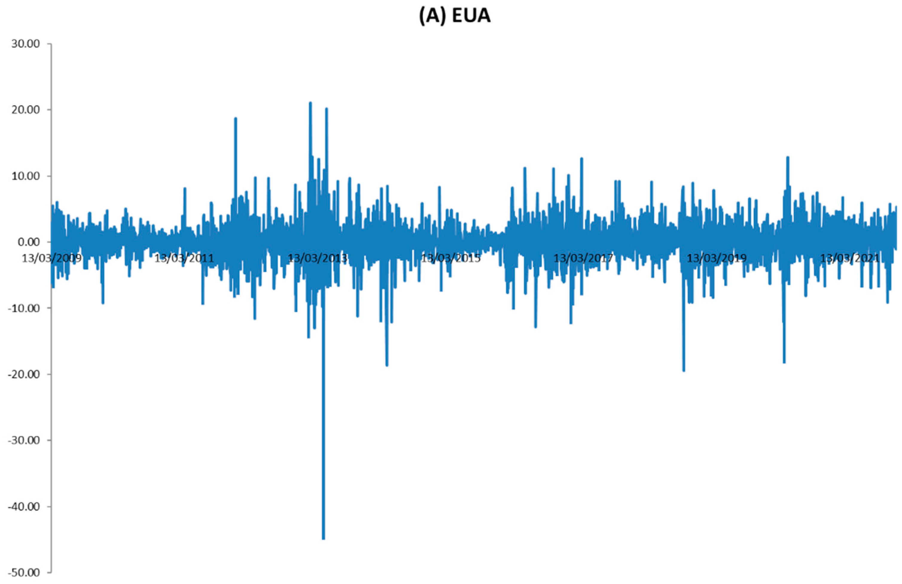
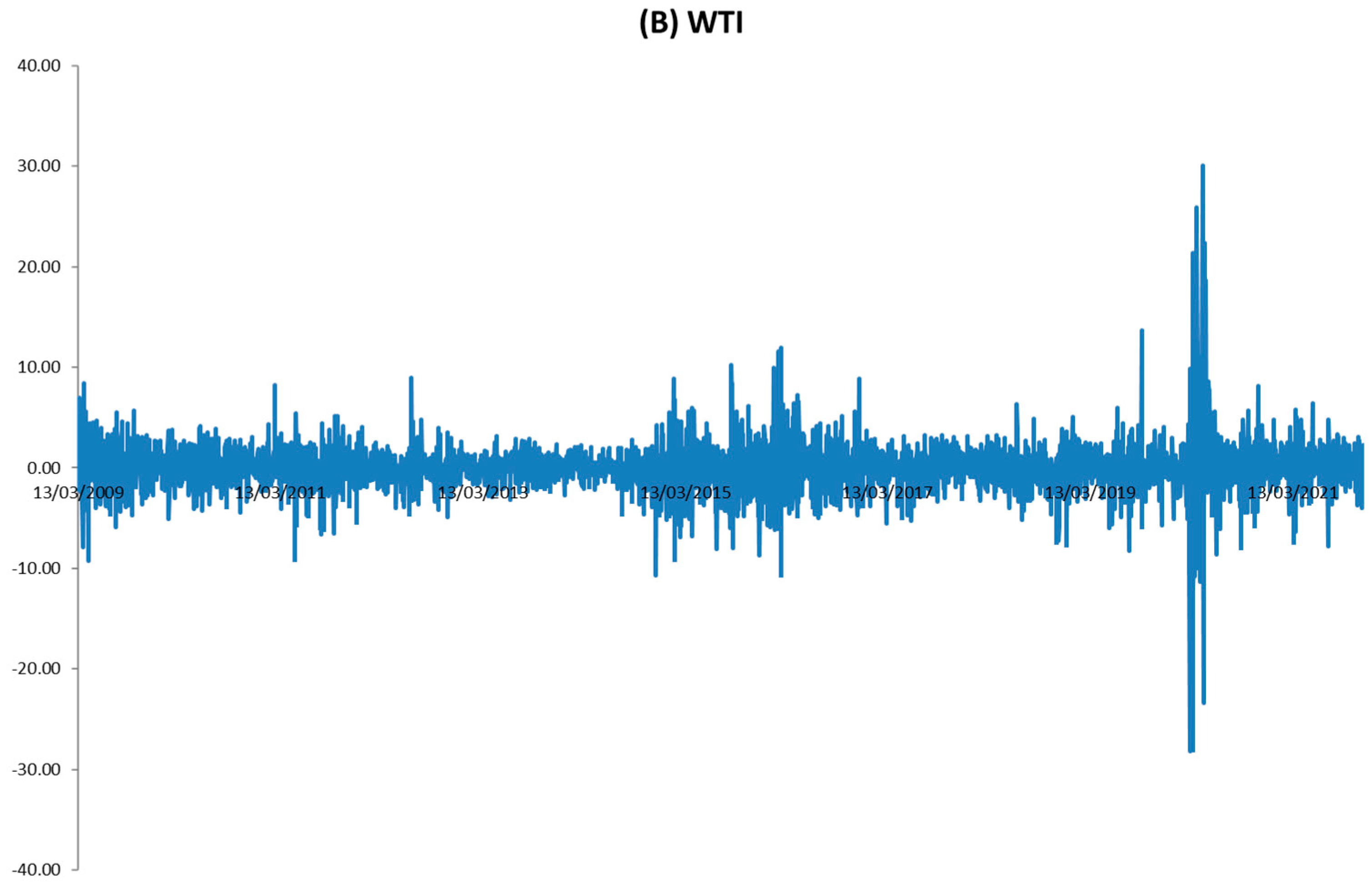
4.3. Illustration of Volatility Jumps

Figure 1 graphs the daily return rate series of EUA and WTI. To illustrate volatility regimes, we use a 21-trading-day rolling window to calculate their volatilities and graph them in Figure 2. The figure shows that return volatilities on EUA and WTI are non-constant and show some specific peaks (i.e., prominent movements). These peaks offer evidence of volatility regimes (i.e., HV versus LV) in carbon–energy markets. For instance, the peak identified in May 2020 corresponds to the economic and financial distresses due to the COVID-19 pandemic.

4.4. Bivariate GARCH Model

Table 3. Estimated results of the bivariate GARCH-CCC model.

	Coefficient	S.D.	t-Statistic	p-Value
EUA Equation
µEUA	0.1290	0.0358	3.6034	0.0002
φEUA	−0.0037	0.0032	−1.1563	0.1238
ωEUA	0.1047	0.0241	4.3444	0.0000
αEUA	0.1226	0.0110	11.1455	0.0000
βEUA	0.8777	0.0102	86.0490	0.0000
WTI Equation
µWTI	0.0937	0.0268	3.4963	0.0002
φWTI	0.0036	0.0131	0.2748	0.3917
ωWTI	0.1687	0.0327	5.1590	0.0000
αWTI	0.1370	0.0120	11.4167	0.0000
βWTI	0.8393	0.0143	58.6923	0.0000
Correlation
ρ	0.1716	0.0167	10.2754	0.0000
Log-likelihood function		−14,890.8106

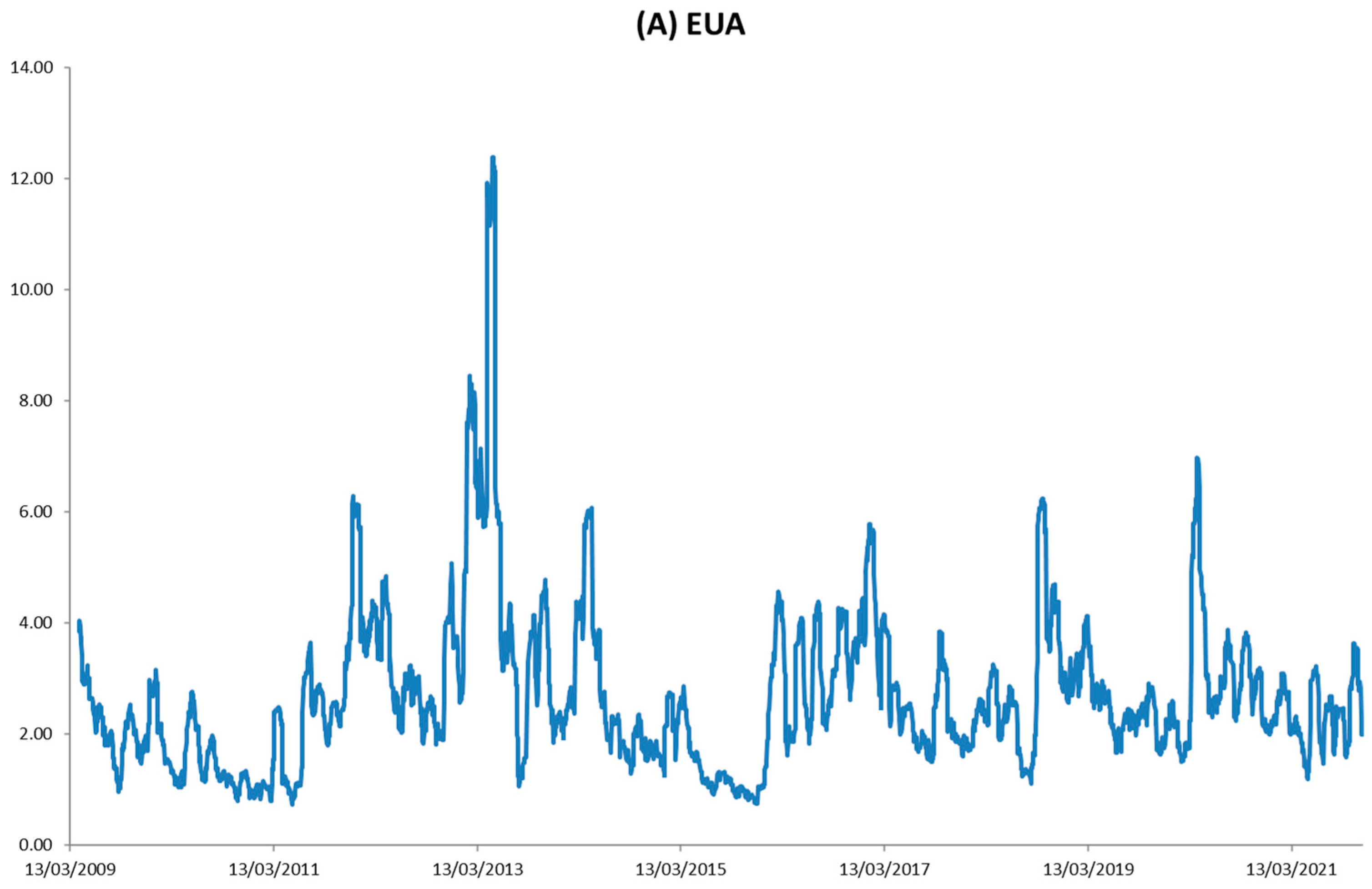
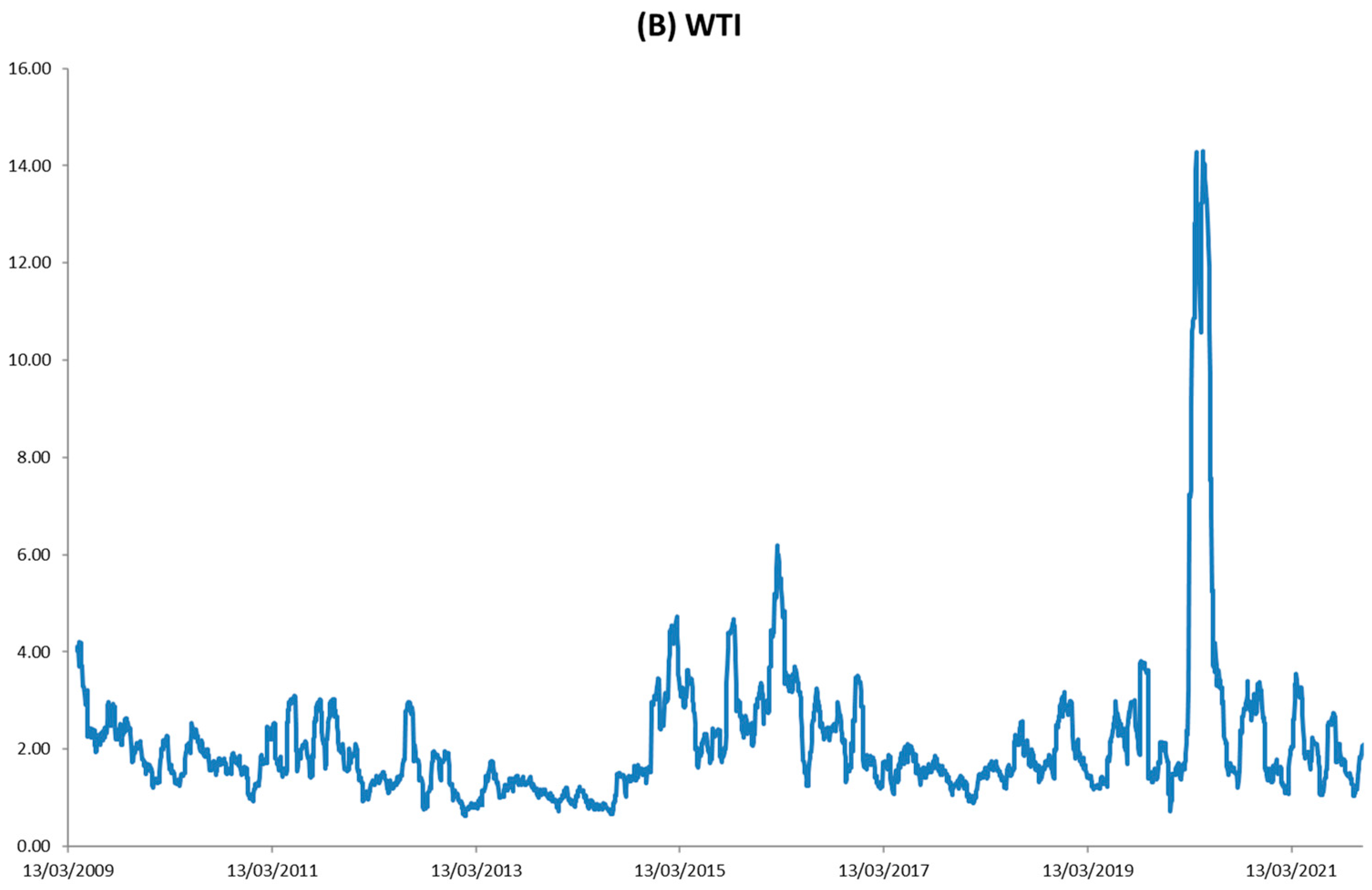
Notes: This table presents the estimation results of the bivariate GARCH-CCC model for EUA and WTI returns. See Table 1 for sample descriptions and data sources.

presents the estimated results of the bivariate GARCH-CCC model. The two estimated GARCH parameters (α^EUA and β^EUA for EUA, and α^WTI and β^WTI for WTI) are positive and significant (p-value < 1%). These results support non-constant volatilities in carbon–energy markets. Notably, the sum of the two estimated GARCH parameters is near to unity (e.g., α^EUA = 0.1226 and β^EUA = 0.8777). This result implies a volatility-clustering phenomenon in the GARCH-based volatility, in that a high/low volatility follows another high/low volatility.

4.5. DCC Model

To examine carbon–energy correlation dynamics, we incorporate the DCC setting into the bivariate GARCH model and present the estimated results in

Table 4. Estimated results of the bivariate GARCH-DCC model.

	Coefficient	S.D.	t-Statistic	p-Value
EUA Equation
µEUA	0.1122	0.0383	2.9295	0.0017
φEUA	−0.0159	0.0085	−1.8706	0.0307
ωEUA	0.0840	0.0221	3.8009	0.0001
αEUA	0.1037	0.0107	9.6916	0.0000
βEUA	0.8949	0.0103	86.8835	0.0000
WTI Equation
µWTI	0.0607	0.0348	1.7443	0.0406
φWTI	−0.0196	0.0105	−1.8667	0.0310
ωWTI	0.1033	0.0232	4.4526	0.0000
αWTI	0.0991	0.0100	9.9100	0.0000
βWTI	0.8838	0.0118	74.8983	0.0000
Time-varying correlation
τ	0.0026	0.0016	1.6250	0.0521
π	0.9751	0.0102	95.5980	0.0000
λ	0.0110	0.0035	3.1429	0.0008
Log-likelihood function		−14,834.1637

Notes: This table presents the estimation results of the bivariate GARCH-DCC model for EUA and WTI returns. See Table 1 for sample descriptions and data sources.

. The table shows that the two estimated DCC parameters, π and λ, are positive and significant (p-value < 0.01). This result supports the correlation-clustering phenomenon—a high/low correlation follows with another high/low correlation.

4.6. Bivariate SWARCH Model

Table 5. Estimated results of the bivariate SWARCH model with state-varying correlations.

	Coefficient	S.D.	t-Statistic	p-Value
EUA Equation
p11EUA	0.9729	0.0055	176.8909	0.0000
p22EUA	0.9316	0.0141	66.0709	0.0000
µEUA	0.1138	0.0413	2.7554	0.0029
φEUA	−0.0139	0.0093	−1.4946	0.0675
ωEUA	3.4121	0.1807	18.8827	0.0000
αEUA	0.0242	0.0172	1.4070	0.0797
g2EUA	6.7405	0.4385	15.3717	0.0000
WTI Equation
p11WTI	0.9841	0.0039	252.3333	0.0000
p22WTI	0.9309	0.0164	56.7622	0.0000
µWTI	0.0434	0.0361	1.2022	0.1146
φWTI	−0.0262	0.0153	−1.7124	0.0434
ωWTI	2.2234	0.1218	18.2545	0.0000
αWTI	0.1704	0.0286	5.9580	0.0000
g2WTI	8.1736	0.8642	9.4580	0.0000
State-varying correlations
ρ1,1	0.1751	0.0255	6.8667	0.0000
ρ2,1	0.1109	0.0391	2.8363	0.0023
ρ1,2	0.2977	0.0556	5.3543	0.0000
ρ2,2	0.3609	0.0637	5.6656	0.0000
LRstatisticforρ1,1 = ρ2,1 = ρ1,2 = ρ2,2		15.0222 ***
Log-likelihood function		−14,890.1349

Notes: This table presents the estimation results of the bivariate SWARCH model with state-varying correlations for EUA and WTI returns. To test the significance, we implement an identical correlation, i.e., ρ_1,1 = ρ_2,1 = ρ_1,2 = ρ_2,2 = ρ, into the model and calculate the value of the log-likelihood function of the restricted model. Then, we use the difference between the two models (one with four-state correlations vs. one with an identical correlation) to develop the likelihood ratio (LR) statistic. The LR statistic follows a chi-square distribution with three (=4 − 1) degrees of freedom. *** denotes significance at the 1% level. See Table 1 for sample descriptions and data sources.

presents the estimated results of the bivariate SWARCH model with state-varying correlations. This model employs a regime-switching approach to address the non-uniform volatility–correlation relationships that may help us re-examine the intensity and direction of the volatility spillover effect in carbon–energy markets (see Section 2.2). First, the estimated volatility scale parameters (i.e., g₂^EUA and g₂^WTI) are significantly larger than the unity. In particular, g₂^EUA is 6.7405, and its standard deviation is 0.4385. Moreover, g₂^WTI is 8.1736, and its standard deviation is 0.8642. Since their 99% confidence intervals do not cover the value of one (g₁^EUA = g₁^WTI = 1), we recognize Regime II as a high-volatility (HV) regime and Regime I as a low-volatility (LV) regime.

Second, as shown in Table 5, all the estimated correlations (i.e., ρ_1,1, ρ_2,1, ρ_1,2, and ρ_2,2) are positive and significant (p-value < 1%) but display considerable divergence. Moreover, the assumption of an equal correlation (i.e., ρ_1,1 = ρ_2,1 = ρ_1,2 = ρ_2,2 = ρ) is rejected at a 1% significance level. These results confirm the non-uniform correlations across various volatility regimes in carbon–energy markets.

5. Discussion and Practical Tests

5.1. Volatility Spillover Effect: Intensity and Direction

In addition to research modeling, this study uses the volatility–correlation relationships to re-detect the intensity and direction of the volatility spillover effect in carbon–energy markets (see Section 2.2). Figure 2 graphs the estimated probabilities of various volatility states derived by the bivariate SWARCH model. To identify the specific state for each point in time, we use a maximum value criterion. Specifically, if the HV-HV state’s estimated probability is higher than that of the other three states, we define this point in time as an HV-HV state. Next, the observation percentage for each volatility state is calculated and presented in

Table 6. Observation percentage of various volatility states.

	Observation Percentage
EUA = LV and WTI = LV	64.54%
EUA = HV and WTI = LV	19.98%
EUA = LV and WTI = HV	11.00%
EUA = HV and WTI = HV	4.50%
Total	100%

Notes: One key feature of the bivariate SWARCH model employed in this study is to provide the estimated probabilities of a specific state for each time point. We use these estimated probabilities and a maximum value criterion to define the volatility state. For example, if the HV-HV state’s estimated probability is higher than the other three states, we identify this time point as an HV-HV state.

. First, the state of EUA = LV and WTI = LV (LV-LV) is the most common (64.54%), whereas the state of EUA = HV and WTI = HV (HV-HV) is the most uncommon (4.50%). Last, 19.98% of the observations are identified as the state of EUA = HV and WTI = LV (HV-LV) and the state of EUA = LV and WTI = HV (LV-HV) is identified in 11.00% of our observations.

Next, we conduct two comparative analyses to examine the intensity and direction of the volatility spillover effect. The first comparative analysis is based on LV-LV versus HV-HV. Under the LV-LV state, the volatility spillover effect becomes minimal because both EUA (carbon market) and WTI (energy market) face a low-volatility regime. Thus, the carbon–energy correlation is mainly driven by the fundamental channel. On the other hand, the volatility spillover effect becomes maximal under the HV-HV state. Accordingly, the carbon–energy correlation under the HV-HV state reflects both the fundamental channel and the volatility spillover effect. Returning to Table 5, ρ_1,1 is 0.1751 (or 17.51%) and ρ_2,2 is 0.3609 (or 36.09%). The rise in the correlation from the LV-LV state to the HV-HV state reflects the intensity of the volatility spillover effect in carbon–energy markets.

We use the other two volatility states to conduct the second comparative analysis, which may detect the direction of the volatility spillover effect. As shown in Table 5, ρ_2,1 is 0.1109 and ρ_1,2 is 0.2977. The comparison shows that a higher carbon–energy correlation is observed when the energy market (proxied by WTI) faces an HV regime rather than the carbon market (proxied by EUA). This result implies that the volatility spillover direction is from the energy market to the carbon market (e.g., Tang and Wang, 2017).

5.2. Portfolio Risk Forecasting

This section conducts our first practical test: portfolio risk forecasting. The risk of a portfolio involves two key elements: volatilities and correlations. This study employs various models for dynamic carbon–energy volatilities and correlations, including the GARCH, DCC, and SWARCH models. The question arises: would state-dependent volatilities and correlations involved in our bivariate SWARCH model help with portfolio risk forecasting, compared with the simple time-dependent volatilities and correlations in the conventional bivariate GARCH and DCC models?

To answer this question, we construct the equal-weighted energy–carbon volatilities and correlations for each of the three models (bivariate GARCH-CCC, bivariate GARCH-DCC, and bivariate SWARCH); we then calculate the model-implied variance of portfolio return residuals at each time t over the sample period. It should be noted that, since there are four different volatility state combinations at time t in our bivariate SWARCH model, we first compute the model-implied standard deviation for each volatility state (i.e., LV-LV, HV-LV, LV-HV, and HV-HV) and then determine the weighted average standard deviation based on the probabilities of realizing the four state combinations.

We calculate MAE (Mean Absolute Error) and MSE (Mean Square Error), the two most prominent forecasting performance measures, for each model and present the results in

Table 7. Performance of EUA–WTI portfolio variance forecasting.

	MAE
Panel A: MAE (Mean Absolute Error)
Bivariate GARCH-CCC model	2.3185
Bivariate GARCH-DCC model	2.3143 (−1.0906)
Bivariate SWARCH model with state-varying correlations	2.1470 (−8.9225) ***
Panel B: MAE (Mean Square Error)
Bivariate GARCH-CCC model	9.9811
Bivariate GARCH-DCC model	9.9981 (0.3579)
Bivariate SWARCH model with state-varying correlations	8.5664 (−5.5544) ***

Notes: This study adopts MSE and MAE, the two commonly used forecasting performance criteria, to evaluate the performance of various models in EUA–WTI portfolio variance forecasting. We adopt the bivariate GARCH-CCC model as a benchmark and calculate the statistic for the difference in MSE and MAE (see the figure in parenthesis). *** represents significance at the 1% level.

. The table shows that the bivariate SWARCH model with state-varying correlations is associated with the smallest MSE and MAE. Moreover, we use the GARCH-CCC model as a benchmark to calculate the t-statistic for the difference in MSE and MAE. Notably, the statistic is significant at 1% for the SWARCH model. Our conclusion is clear. Our proposed regime-switching volatilities and correlations may help with EUA–WTI portfolio risk forecasting.

The MSE and MAE are defined as follows:

$$MSE=T^{-1}{\sum }_{t=1}^T{(r_{p,t}^2-{\sigma }_{p,t}^2)}^2, MAE=T^{-1}{\sum }_{t=1}^T|r_{p,t}^2-{\sigma }_{p,t}^2|$$

where r_p,t is the return of the equal-weight portfolio of energy and carbon at time t, and σ_p,t is the estimated standard deviation of the respective carbon–energy portfolio return residuals according to each of the models.

5.3. Portfolio Construction

This section conducts our second practical test: portfolio construction. Again, portfolio construction relies on volatilities and correlations. A direct question we ask is if our proposed regime-switching approach may enhance portfolio construction effectiveness. To answer this question, we run a test and detail the test as follows: First, we employ a minimum variance portfolio construction strategy [46,47]. In this strategy, the weight given to each position in the EUA–WTI portfolio is calculated as follows:

$$w_t^{EUA}=\left[h_t^{WTI}-{\rho }_t{\left(h_t^{EUA}·h_t^{WTI}\right)}^{1/2}]/[h_t^{EUA}+h_t^{WTI}-2·{\rho }_t{\left(h_t^{EUA}·h_t^{WTI}\right)}^{1/2}\right]$$

(16)

$$w_t^{WTI}=1-w_t^{EUA}$$

(17)

where w_t^EUA and w_t^WTI represent the weight of EUA (carbon) and WTI (energy) asset position, respectively. h_t^EUA and h_t^WTI denote the conditional variances of EUA and WTI, respectively, and ρ_t is their correlation.

Second, we construct the portfolio and calculate the portfolio return at time t (r_t^POT):

$$r_t^{POT}=w_t^{EUA}·r_t^{EUA}+w_t^{WTI}·r_t^{WTI}$$

(18)

Finally, we calculate the portfolio’s return mean and volatility over the testing period.

Table 8. Performance of EUA–WTI portfolio construction.

Panel A: Portfolio mean return
	Mean return
Bivariate GARCH-CCC model	0.0436
Bivariate GARCH-DCC model	0.0427 (−0.3524)
Bivariate SWARCH model with state-varying correlations	0.0452 (0.1611)
Panel B: Portfolio return volatility
	Return volatility
Bivariate GARCH-CCC model	1.7981
Bivariate GARCH-DCC model	1.7840 (−1.5996)
Bivariate SWARCH model with state-varying correlations	1.6392 (−7.2752) ***
Panel C: Sharpe ratios
	Sharpe ratio
Bivariate GARCH-CCC model	0.0242
Bivariate GARCH-DCC model	0.0239
Bivariate SWARCH model with state-varying correlations	0.0276

Notes: This table lists the performance of portfolio construction (via a minimum variance strategy) for each model. Two portfolio performance measures are adopted: mean return and return volatility. We use the bivariate GARCH-CCC model as a benchmark to calculate the t-statistic for the difference (the figure in the parenthesis). *** denotes significance at the 1% level.

presents the results for each model. To test significance, the bivariate GARCH-CCC model is used as a benchmark to calculate the t-statistic for the difference between alternative models. As shown in Table 8, our proposed bivariate SWARCH model equipped with state-dependent correlations constructs a carbon–energy portfolio with a higher mean return and lower return volatility than the bivariate GARCH-CCC and -DCC models. Notably, the difference in the portfolio’s mean return is insignificant (p-value > 10%), whereas the difference in the portfolio’s return volatility is significant (p-value < 1%).

5.4. Issue of COVID-19 Pandemic

The issue of the COVID period is critical. As shown in Figure 2, a peak is identified in May 2020, corresponding to the economic and financial distresses due to the COVID-19 pandemic. To test if the issue of the COVID-19 pandemic affects our conclusion, we exclude the data after 2020 and rerun the models. The results are consistent with the following notions: First, g₂^EUA is 7.0437, and its standard deviation is 0.4887. Moreover, g₂^WTI is 4.4603, and its standard deviation is 0.3060. These results imply Regime II (I) as a high (low)-volatility regime, consistent with Table 5. Second, ρ_2,2 (0.2363) is higher than ρ_1,1 (0.1083), implying the intensity of the volatility spillover effect in carbon–energy markets. Third, ρ_1,2 (0.3418) is higher than ρ_2,1 (0.0979), which means that the volatility spillover direction is from the energy market to the carbon market. Overall, our conclusion on the intensity and direction of volatility spillover effect in carbon–energy markets is robust to the subperiod. However, as shown in Table 5, the estimate of ρ_2,2 is 0.3609, which is higher than all the correlation estimates obtained with the subperiod data. The result implies the COVID-19 pandemic enlarges carbon–energy market volatilities and correlations.

6. Conclusions and Future Research Directions

The volatility spillover effect in carbon–energy markets has been documented in the literature. Our study offers contributions to the literature in three respects. First, we develop the non-uniform volatility–correlation relationships and use them to re-examine the intensity and direction of the volatility spillover effect in carbon–energy markets. Second, we develop a bivariate SWARCH model with four-state volatility combinations and correlations. Third, we employ the realized data (EUA and WTI) to run the model empirically using a one-step estimation process. Finally, we perform two practical tests, portfolio volatility forecasting and portfolio construction, to validate our proposed regime-switching approach.

Using a two-volatility-state setting for each carbon and energy market (HV versus LV), we establish a four-volatility-state system for carbon–energy markets (i.e., LV-LV, HV-LV, LV-HV, and HV-HV). We then develop the non-uniform volatility–correlation relationships using these volatility state groupings. While existing studies have provided evidence of the volatility spillover effect in carbon–energy markets, to the best of our knowledge, they have neither addressed the non-uniform volatility–correlation relationships, nor used them to empirically prove the intensity and direction of the volatility spillover effect. We fill these gaps by developing a theoretical hypothesis, constructing a specific econometric method, and conducting two practical risk management tests.

Our empirical findings are presented as follows: First, the carbon–energy correlation under the HV-HV state is larger than that under the LV-LV state. This result offers evidence of the volatility spillover effect in carbon–energy markets. Second, when the carbon and energy markets are experiencing an opposite volatility regime (i.e., one in an HV regime and the other in an LV regime), a higher carbon–energy correlation is observed when the energy market is in an HV regime. This result indicates that the direction of the volatility spillover effect is from the energy market to the carbon market. Third, our proposed regime-switching approach may offer better performance on carbon–energy portfolio risk forecasting and portfolio construction than the conventional GARCH and DCC models.

Lastly, we address several future research directions. First, this study uses the equal-weighted carbon–energy portfolio for the portfolio risk forecasting test (Section 5.2) and the minimum variance portfolio for the portfolio construction test (Section 5.3). Future research may consider value-weighted portfolios. Second, to address the non-normality distribution issue, one may incorporate non-normal distributions, such as the t-distribution or the GED distribution, into the models [48,49].

References

1. Michaelowa, A.; Michaelowa, K.; Shishlov, I.; Brescia, D. Catalysing private and public action for climate change mitigation: The World Bank’s role in international carbon markets. Clim. Policy 2021, 21, 120–132. [Google Scholar] [CrossRef]
2. Gong, X.; Shi, R.; Xu, J.; Lin, B. Analyzing spillover effects between carbon and fossil energy markets from a time-varying perspective. Appl. Energy 2021, 285, 116384. [Google Scholar] [CrossRef]
3. Chevallier, J. Time-varying correlations in oil, gas and CO2 prices: An application using BEKK, CCC and DCC-MGARCH models. Appl. Econ. 2012, 44, 4257–4274. [Google Scholar] [CrossRef] [Green Version]
4. Zhang, Y.J.; Sun, Y.F. The dynamic volatility spillover between European carbon trading market and fossil energy market. J. Clean. Prod. 2016, 112, 2654–2663. [Google Scholar] [CrossRef]
5. Lin, B.; Chen, Y. Dynamic linkages and spillover effects between CET market, coal market and stock market of new energy companies: A case of Beijing CET market in China. Energy 2019, 172, 1198–1210. [Google Scholar] [CrossRef]
6. Li, L. The dynamic interrelations of oil-equity implied volatility indexes under low and high volatility-of-volatility risk. Energy Econ. 2022, 105, 105756. [Google Scholar] [CrossRef]
7. Li, L.; Scrimgeour, F. The co-integration of CDS and bonds in time-varying volatility dynamics: Do credit risk swaps lower bond risks? Stud. Nonlinear Dyn. Econom. 2022, 26, 475–497. [Google Scholar] [CrossRef]
8. Heckman, J. Sample selection bias as a specification error. Econometrica 1979, 47, 153–161. [Google Scholar] [CrossRef]
9. Tan, X.; Sirichand, K.; Vivian, A.; Wang, X. How connected is the carbon market to energy and financial markets? A systematic analysis of spillovers and dynamics. Energy Econ. 2020, 90, 104870. [Google Scholar] [CrossRef]
10. Chevallier, J. A model of carbon price interactions with macroeconomic and energy dynamics. Energy Econ. 2011, 33, 1295–1312. [Google Scholar] [CrossRef]
11. Tan, X.; Wang, X. Dependence changes between the carbon price and its fundamentals: A quantile regression approach. Appl. Energy 2017, 190, 306–325. [Google Scholar] [CrossRef]
12. Zhao, X.; Han, M.; Ding, L.L.; Kang, W.L. Usefulness of economic and energy data at different frequencies for carbon price forecasting in the EU ETS. Appl. Energy 2018, 216, 132–141. [Google Scholar] [CrossRef]
13. Lin, B.; Jia, Z. Impacts of carbon price level in carbon emission trading market. Appl. Energy 2019, 239, 157–170. [Google Scholar] [CrossRef]
14. Liu, H.; Chen, Y. A study on the volatility spillovers, long memory effects and interactions between carbon and energy markets: The impacts of extreme weather. Econ. Model. 2013, 35, 840–855. [Google Scholar] [CrossRef]
15. Koch, N. Dynamic linkages among carbon, energy and financial markets: A smooth transition approach. Appl. Econ. 2014, 46, 715–729. [Google Scholar] [CrossRef]
16. Balcılar, M.; Demirer, R.; Hammoudeh, S.; Nguyen, D.K. Risk spillovers across the energy and carbon markets and hedging strategies for carbon risk. Energy Econ. 2016, 54, 159–172. [Google Scholar] [CrossRef] [Green Version]
17. Byun, S.J.; Cho, H. Forecasting carbon futures volatility using GARCH models with energy volatilities. Energy Econ. 2013, 40, 207–221. [Google Scholar] [CrossRef]
18. Wei, C.C.; Lin, Y.G. Carbon future price return, oil future price return and stock index future Price return in the US. Int. J. Energy Econ. Policy 2016, 6, 655–662. [Google Scholar]
19. Lin, B.; Li, J. The spillover effects across natural gas and oil markets: Based on the VEC-MGARCH framework. Appl. Energy 2015, 155, 229–241. [Google Scholar] [CrossRef]
20. Wang, Y.; Guo, Z. The dynamic spillover between carbon and energy markets: New evidence. Energy 2018, 149, 24–33. [Google Scholar] [CrossRef]
21. Diebold, F.X.; Yilmaz, K. Better to give than to receive: Predictive directional measurement of volatility spillovers. Int. J. Forecast. 2012, 28, 57–66. [Google Scholar] [CrossRef] [Green Version]
22. Ji, Q.; Zhang, D.; Geng, J. Information linkage, dynamic spillovers in prices and volatility between the carbon and energy markets. J. Clean. Prod. 2018, 198, 972–978. [Google Scholar] [CrossRef]
23. Diebold, F.X. Modeling the persistence of conditional variance: A comment. Econom. Rev. 1986, 5, 51–56. [Google Scholar] [CrossRef]
24. Lamoureux, C.G.; Lastrapes, W.D. Persistence in variance, structural change and the GARCH model. J. Bus. Econ. Stat. 1990, 8, 225–234. [Google Scholar]
25. Aielli, G.P. Dynamic conditional correlation: On properties and estimation. J. Bus. Econ. Stat. 2013, 31, 282–299. [Google Scholar] [CrossRef]
26. Kodres, L.; Pritsker, M. A rational expectations model of financial contagion. J. Financ. 2002, 57, 769–800. [Google Scholar] [CrossRef] [Green Version]
27. Trevino, I. Informational channels of financial contagion. Econometrica 2020, 88, 297–335. [Google Scholar] [CrossRef]
28. Engle, R.; Ghysels, E.; Sohn, B. Stock market volatility and macroeconomic fundamentals. Rev. Econ. Stat. 2013, 95, 776–797. [Google Scholar] [CrossRef]
29. Baker, S.R.; Bloom, N.; Davis, S.J. Measuring economic policy uncertainty. Q. J. Econ. 2016, 131, 1593–1636. [Google Scholar] [CrossRef]
30. Gulen, H.; Ion, M. Policy uncertainty and corporate investment. Rev. Financ. Stud. 2016, 29, 523–564. [Google Scholar] [CrossRef]
31. Danielsson, J.; Valenzuela, M.; Zer, I. Learning from history: Volatility and financial crises. Rev. Financ. Stud. 2018, 31, 2774–2805. [Google Scholar] [CrossRef]
32. Li, L. Dynamic correlations and domestic-global diversification. Res. Int. Bus. Financ. 2017, 39, 280–290. [Google Scholar] [CrossRef]
33. Li, L. Testing and comparing the performance of dynamic variance and correlation models in value-at-risk estimation. N. Am. J. Econ. Financ. 2017, 40, 116–135. [Google Scholar] [CrossRef]
34. Engle, R.F. Dynamic conditional correlation: A simple class of multivariate generalized autoregressive conditional heteroskedasticity models. J. Bus. Econ. Stat. 2002, 20, 339–350. [Google Scholar] [CrossRef]
35. Gray, S.F. Modeling the conditional distribution of interest rates as a regime-switching process. J. Financ. Econ. 1996, 42, 27–62. [Google Scholar] [CrossRef]
36. Dueker, M.J. Markov switching in GARCH processes and mean-reverting stock-market volatility. J. Bus. Econ. Stat. 1997, 15, 26–35. [Google Scholar]
37. Klaassen, F. Improving GARCH volatility forecasts with regime-switching GARCH. Empir. Econ. 2002, 27, 363–394. [Google Scholar] [CrossRef] [Green Version]
38. Smith, D.R. Markov-switching and stochastic volatility diffusion models of short-term interest rates. J. Bus. Econ. Stat. 2002, 20, 183–197. [Google Scholar] [CrossRef]
39. Augustyniak, M. Maximum likelihood estimation of the Markov-switching GARCH model. Comput. Stat. Data Anal. 2014, 76, 61–75. [Google Scholar] [CrossRef]
40. Ramchand, L.; Susmel, R. Volatility and cross-correlation across major stock markets. J. Empir. Financ. 1998, 5, 397–416. [Google Scholar] [CrossRef]
41. Edwards, S.; Susmel, R. Interest-rate volatility in emerging markets. Rev. Econ. Stat. 2003, 85, 328–348. [Google Scholar] [CrossRef]
42. Dickey, D.A.; Fuller, W.A. Likelihood ratio statistics for autoregressive time series with a unit root. Econometrica 1981, 49, 1057–1072. [Google Scholar] [CrossRef]
43. Phillips, P.C.B.; Perron, P. Testing for a unit root in a time series regression. Biometrika 1988, 75, 335–346. [Google Scholar] [CrossRef]
44. Elliott, G.; Rothenberg, T.J.; Stock, J.H. Efficient tests for an autoregressive unit root. Econometrica 1996, 64, 813–836. [Google Scholar] [CrossRef] [Green Version]
45. Ng, S.; Perron, P. Lag length selection and the construction of unit root tests with good size and power. Econometrica 2001, 69, 1519–1554. [Google Scholar] [CrossRef] [Green Version]
46. French, K.R.; Poterba, J.M. Investor diversification and international equity markets. Am. Econ. Rev. 1991, 81, 222–226. [Google Scholar]
47. Tesar, L.L.; Werner, I. Home Bias and the Globalization of Securities Markets; National Bureau of Economic Research: Cambridge, UK, 1992. [Google Scholar]
48. Deng, X.; Yao, J. On the property of multivariate generalized hyperbolic distribution and the Stein-type inequality. Commun. Stat. Theory Methods 2018, 47, 5346–5356. [Google Scholar] [CrossRef]
49. Li, L.; Lin, W. Examining the volatility of Taiwan stock index returns via a three-volatility-regime Markov-switching ARCH model. Rev. Quant. Financ. Account. 2003, 21, 123–139. [Google Scholar] [CrossRef]
Figure 1. Return rates on EUA carbon price and WTI crude oil price.
Algorithms 15 00264 g001aAlgorithms 15 00264 g001b
Figure 2. Volatility of return rates on EUA carbon price and WTI crude oil price.
Algorithms 15 00264 g002aAlgorithms 15 00264 g002b