Trinity: Neural Network Adaptive Distributed Parallel Training Method Based on Reinforcement Learning

Abstract

Deep learning, with increasingly large datasets and complex neural networks, is widely used in computer vision and natural language processing. A resulting trend is to split and train large-scale neural network models across multiple devices in parallel, known as parallel model training. Existing parallel methods are mainly based on expert design, which is inefficient and requires specialized knowledge. Although automatically implemented parallel methods have been proposed to solve these problems, these methods only consider a single optimization aspect of run time. In this paper, we present Trinity, an adaptive distributed parallel training method based on reinforcement learning, to automate the search and tuning of parallel strategies. We build a multidimensional performance evaluation model and use proximal policy optimization to co-optimize multiple optimization aspects. Our experiment used the CIFAR10 and PTB datasets based on InceptionV3, NMT, NASNet and PNASNet models. Compared with Google’s Hierarchical method, Trinity achieves up to 5% reductions in runtime, communication, and memory overhead, and up to a 40% increase in parallel strategy search speeds.

1. Introduction

In recent years, with the rapid development of AI algorithms, hardware computing power, and dataset development, deep learning has been widely used in various fields, such as natural language processing [1,2], computer vision [3,4], and search recommendation [5,6]. Deep learning technologies rely on deep and complex neural networks and large-scale datasets. For example, BERT-Large [7], a transformer with 400 million parameters, occupies over 32 GB of memory; and GPT-3 [8], with 175 billion parameters, occupies over 350 GB of memory. Due to the limited computing power and storage capacity of the hardware, a single device cannot process such large-scale models and datasets. Therefore, it is necessary to divide the large-scale neural network into multiple submodels and schedule them on different devices (CPU and GPU) for execution, a procedure known as model parallel training.

Previously, parallel strategies were designed by expert experience [9,10,11]. They usually dispatch the submodels of networks onto different devices for execution, preserving the spatial nature of the original model as much as possible, and balancing the computing and communication overhead.

For example, Wu [12] and Sutskever et al. [13] dispatched the LSTM layer, attention layer, and softmax layer onto different devices for execution. However, imbalanced memory uptake and computing costs between layers still present challenges for certain devices. To solve these problems, researchers have proposed segmentation methods based on the granularity of the operator. For instance, Sun et al. [14] used skeleton networks to achieve the random partition of the network and reduce redundancy. Ballard [15] and Demmel et al. [16] further introduced high-performance computing (HPC) matrix portion methods to achieve fine-grained parallelism for matrix multiplication operations inside operators. However, as the granularity of the division becomes finer, the distributed combinations increase exponentially [17]. It is also challenging to find an optimal parallel strategy using expert experience, which requires knowledge in many fields, such as deep learning, distributed computing and computer architecture; and it is difficult to generalize an optimal parallel strategy to other networks.

To address these challenges, researchers proposed automated frameworks for finding efficient parallelization strategies in a limited search space. These frameworks can be roughly divided into two types: one is based on graph algorithms [18,19,20,21,22,23,24,25] and the other type is based on machine learning [17,26,27,28,29,30,31]. For the former, Pellegrini et al. [18] followed HPC, and proposed Scotch, a method to partition static graphs, including Multilevel Method [20], k-way Fiduccia–Mattheyses (Fiduccia Mattheyses) [32], and RPM Recursive Bipartitioning Mapping [18]. Although these methods balance the communication workloads, they cannot be directly applied to dynamic environments. Jia et al. [21] proposed FlexFlow, a deep learning framework that uses the guided randomized search of the search space to find a fast parallelization strategy for a specific parallel machine. Peng et al. [22] built a performance model for Parameter Server (PS) [33,34,35]) and minimized the job training time based on predicting the training speed. Tofu [23] considered a similar problem, using dynamic programming to automatically split dataflow graphs and minimize the total communication costs. However, these approaches have limitations. FlexFlow is suitable only for DNNs, Optimus is only based on a PS, and Tofu only considers the minimal communication overhead. Moreover, their parallel strategy search space usually grows exponentially. Therefore, these limitations make them difficult to further promote.

In addition to graph algorithms, the successful experience of machine learning in the field of systems and resource scheduling has prompted researchers to use machine learning to solve neural network segmentation and scheduling problems. Kim et al. [26] proposed Parallex, a learning linear model that adjusts the size of variables to achieve adaptive tensor partitioning. Frazier et al. [27] determined the credit size for scheduling using Bayesian optimization. However, these two methods are based on traditional machine learning, where the main body tuning model is relatively simple, and the performance of parallel execution is limited. With the development of deep reinforcement learning, Mirhoseini et al. [17] predicted the placement of operations in a neural network based on reinforcement learning. As this method requires the manual grouping of operators, Mirhoseini et al. [28] further proposed Hierarchical, an end-to-end hierarchical architecture that uses Grouper to automatically group computer graph operators and uses Placer to select the best execution equipment for each group of operators. Gao et al. [29] introduced the method of minimizing the cross-entropy into the sampling process of reinforcement learning to prove the improvement of the upper and lower bounds of the Markov process. Addanki et al. [30] proposed Placeto to learn generalizable device placement policies that can be applied to any graph with a graph neural network (GNN).

Graph algorithm (such as Mesh-TensorFlow, FlexFlow, and GPip) and machine learning (including RL methods) are two mainstream parallel search methods for strategies and they are orthogonal and have different advantages. Graph algorithm methods have less expensive search costs than RL methods, but they need to pay attention to the training details and have to weigh the communication, computation, memory and throughput costs of each tensor and operation. RL methods used a data-driven approach as a search strategy and used rewards to guide learning. Therefore, RL methods cost more than graph algorithm methods, but they do not need to focus on the details of parallel training and can automate the scheduling of executions on arbitrary computational graphs.

Although these methods have increased the upper bounds of the performance optimization, there are still some problems to be improved upon:

(1)

Existing distributed parallel techniques are mainly guided by runtime or communication. The distributed training performance evaluation has a single dimension, which cannot describe the distributed training performance of large-scale learning models in a fine-grained manner.

(2)

The parallel strategy search process relies on the real distributed environment, which is expensive (usually takes several hours or even days).

(3)

Hierarchical and Placeto use the policy gradient method to update the reinforcement learning algorithm with a large variance and low sampling efficiency, which is conducive to algorithm convergence.

In response to the aforementioned problems, this paper proposes Trinity, a deep network adaptive distributed parallel training method based on reinforcement learning, to solve the problem of optimizing large-scale complex neural network partition and schedule strategies.

Our contributions are as follows:

(1)

We qualitatively analyze the characteristics of deep learning large models and establish quantitative evaluation models. In this paper, a quantitative evaluation model is used to describe the execution performance of different distributed parallel strategies under multi-dimensional attributes (such as parameters, samples, operators, etc.), to guide the automatic search and tuning methods of distributed parallel strategies;

(2)

We divided the operators into groups according to their attributes to determine the degree of parallelism and used Node2vec to embed the operations. It can capture the structural characteristics of the neural network and improve the performance limit of the parallel strategy;

(3)

We adopted the proximal policy optimization (PPO) method, which expands the offline learning ability of the policy network and improves the stability and convergence rate of the algorithm to optimize reinforcement learning;

(4)

We introduce a simulator through which the single-step execution time of the distributed parallel strategy can be predicted, and the strategy search process can be decoupled from a real cluster. The experiments show that the search time can be reduced by up to 40% on average.

2. Problem Description

The goal of this paper is to search for an optimal model parallel strategy in a high-dimensional space based on reinforcement learning for large-scale deep learning models. Mainstream frameworks such as TensorFlow and Pytorch run neural networks in the form of data flow graphs. Thus, we first define the optimization objective of this paper based on the data flow graph.

2.1. Optimization Objective

The goal of Trinity is to search for a model parallel strategy that optimizes training performance based on reinforcement learning. We first establish a directed acyclic computational graph and device topology diagram based on the neural network data flow and cluster topology, and give the optimization objective.

Definition 1

(Computational Graph $\mathcal{G}(O,E)$). According to the deep learning data flow, define the computational graph $G(O,E)$. O represents the operator sets, and the node $o_i\in O$ represents the operator (such as multiple, reshape, and pooling, etc.). E is the set of directed edges between nodes, including the data dependency between operators.

Definition 2

(Device Topology Diagram $\mathcal{D}(V,C)$). According to the cluster device topology information, define the cluster device topology diagram $\mathcal{D}(V,C)$, where the node $v_i\in V$ represents a device (such as CPU or GPU). Edge $c_{ij}=\left(v_i,v_j\right)$ represents the communication between $v_i$ and $v_j$. Communication methods include NVLink, PCIE, etc.

Based on the above definitions, the optimization objectives of this paper are as follows:   

$$\left({\pi }_g,{\pi }_s\right)=argma{x}_{{\pi }_g,{\pi }_s}f(R;\mathcal{G},\mathcal{D}).$$

(1)

where R represents the execution performance of the parallel strategy. We pose the strategy selection as a maximization optimization problem f on the condition of given $\mathcal{G}$ and $\mathcal{D}$. The strategy herein can be seen as two parts, namely ${\pi }_g$ and ${\pi }_s$, where ${\pi }_g$ is the partition strategy, which divide the computational graph nodes O into k submodels, denoted as $\mathcal{G}=\{g_1,g_2,\dots ,g_k\}$. Each submodel $g_i$ contains multiple operators, which form disjoint subsets. The partition strategy is denoted as ${\pi }_g$.

${\pi }_s$ is schedule strategy, which schedules the submodels in G to be executed on different devices. The schedule process denoted as ${\pi }_s:=\{s_1,s_2,\dots ,s_k\}$. Intuitively, it can be described as $s_i:=g_i\to d_j$, the correspondence of group and devices.

The goal of Trinity is to search for the strategy combination (partition strategy ${\pi }_g$ and schedule strategy ${\pi }_s$), that can maximize the $R({\pi }_g,{\pi }_s)$ through reinforcement learning. Here, $({\pi }_g,{\pi }_s)$ is the optimal parallel strategy that we seek.

Optimize Formula (1) needs to solve two core problems:

(1)

We need to characterize the performance evaluation model R, evaluate the policy performance, and guide the solution of optimization problems.

(2)

We also need to build an agent optimization model. Use reinforcement learning to solve the optimal value in the model-parallel space.

We then give the definition of model parallelism and analyze the factors that affect the performance of model parallelism.

2.2. Model Parallelism

In this section, we will model the parallel training of the neural network and analyze the main factors that affect its performance, and then explain the main problems to be solved in this paper with mathematical expressions.

The goal of neural network training is the following: minimize the objective function $\mathcal{L}$ by iteratively adjusting the weights of network parameters $\Theta$ according to N training samples $\mathbf{x}={\left\{x_n,y_n\right\}}_{n=1}^N$. This process can be expressed by Equation (2):

$$\underset{\Theta }{min}\mathcal{L}(\mathbf{x};\Theta )·\mathrm{s}.\mathrm{t}.·\mathcal{L}(\mathbf{x};\Theta )=\ell \left({\left\{x_n,y_n\right\}}_{n=1}^N;\Theta \right)+r(\Theta ).$$

(2)

In Equation (2), a structure-including function $r(·)$ places penalties for the intended application on the values that $\Theta$ can take, namely regularization. ℓ captures the nonlinear relationship between neural network model parameters. The model parallel usually solves the scenario that the model scale $\Theta$ is too large, unable to be stored by a single device.

Model parallelism refers to strategies that place different parts of computation in $\mathcal{L}$ in parallel using multiple devices. These can be divided into three different parallel granularities as follows:

(1)

Hierarchical parallelism. When the model is a multi-layer neural network, layers can be scheduled to different devices. The parameters can be synchronized through communication;

(2)

Operator-level parallelism. Scheduling different computing operations to different devices, such as matmul, pooling and reshape;

(3)

Tensor-level parallelism. Partition the big matmul into multiple matmuls over small submatrices, and let each device take care of one part therein.

Our approach focuses on the operator-level, combine the operators into submodels, optimize the group, and schedule strategy of operators. We will then abstract the operator-level parallel process into more general expression, and qualitatively analyze the key factors restricting the improvement of parallel performance.

Now, we suppose that the neural network model is divided into k disjoint submodels, i.e., $\mathcal{L}={\left\{{\mathcal{L}}_k\left({\theta }_k\right)\right\}}_{k=1}^K$. We represent the core information of each sub-model $l_k\left({\mathcal{L}}_k\right)$ by the following triples:   

$${\mathit{Mem}}_k=\left({\mathit{Err}}_k,{\mathit{Mem}}_k^0,Ou{t}_k\right).$$

(3)

where $Er{r}_k$ is the back propagation error of the topmost operator for the parameter update. $Ou{t}_k$ is the activation function value at the bottom of the submodel. $Er{r}_k$ and $Ou{t}_k$ are the intermediate computation results of operators in back propagation and forward propagation, respectively. The successor submodels rely on the intermediate computation results $Er{r}_k$ and $Ou{t}_k$ for subsequent computation. ${Mem}_k^0$ represents the memory of activation, error propagation and edge weights of each layer in the sub-model, except for the propagation error of the topmost operator and the bottom activation function value.

When the device schedules sub-model ${\mathcal{L}}_k$, it will read ${Mem}_k^0$ into the device’s memory. After the sub-model computation is completed, the intermediate results $Er{r}_k$ and $Ou{t}_k$ will be scheduled to the device where other sub-models depend on them. Thus, the device overhead can be modeled as Formula (4):

$${min}_{{\pi }_g,{\pi }_s}{\sum }_{d_i,d_j}^{\mathcal{D}}\left\{\underset{\mathrm{Compute}\mathrm{Cost}}{\underbrace{\sum _{k=1}^K\frac{\mathbb{C}\left({\mathcal{L}}_k\right)}{c_i}}}+\underset{\mathrm{Communication}\mathrm{Cost}}{\underbrace{{\displaystyle \sum _{k=1}^K}\frac{Ou{t}_k+Er{r}_k}{b_{i,j}}}}+\underset{\mathrm{Memory}\mathrm{Cost}}{\underbrace{\sum _{k=1}^K\frac{Me{m}_k^0}{m_i}}}\right\}.$$

(4)

where $\mathcal{D}$ is the number of devices; $\mathbb{C}$ represents the floating-point operands; $c_i$ is the calculation density of the device $d_i$; $b_{i,j}$ indicates the bandwidth between devices $d_i$; and $d_j.$ $m_i$ represents the read and write speed of memory $d_i$.

According to the above Formula (4), the parallel execution performance of the model needs to balance computation costs, communication costs, and memory costs to achieve load balancing in three aspects. At the same time, the performance of the above three aspects will directly affect the training time of the model parallel strategy.

Therefore, the computation costs, communication costs, and memory costs are important factors that determine the performance of the distributed training of neural networks.

Based on the above analysis, we will build an evaluation model that can measure the performance of the model parallelism.

3. Performance Evaluation Model

In this section, we will define the cost model and build the complete performance evaluation model (denoted as the MDPE model) R based on three key factors that affect the efficiency of the parallel execution of the model: computation cost, communication cost, and memory cost (see Definitions 3–5).

Definition 3

(Compute Cost). Define the runtime required for the submodel tensors to complete the computation on device $d_i$ as $E_i$:

$$E_i=\sum _{k=1}^K\frac{\mathbb{C}\left({\mathcal{L}}_k\right)}{c_i}=\sum _{n=1}^N\frac{\mathbb{C}\left({\mathbf{T}}_{n,1},{\mathbf{T}}_{n,2},\dots ,{\mathbf{T}}_{n,k}\right)}{c_i}.$$

(5)

where K represents the number of submodels computed at device $d_i$. N is the total number of tensors involved in the calculation. ${\mathbf{T}}_{n,1},{\mathbf{T}}_{n,2},\dots ,{\mathbf{T}}_{n,k}$ represent the k-dimensional size of the current tensor. $\mathbb{C}$ is the floating-point operands. $c_i$ is the computing density of device $d_i$.

Definition 4

(Communication Cost). Define the communication and synchronization time for intermediate results of the submodel as $C_{i,j}$:

$$C_{i,j}=\sum _{k=1}^K\frac{{\mathit{Out}}_k+Er{r}_k}{b_{i,j}}=\sum _{n=1}^N\frac{\mathbb{A}\left({\mathrm{T}}_n\right)}{b_{i,\mathrm{j}}}s.t.C_{i,j}\le {\widehat{C}}_{i,j}.$$

(6)

where N represents the total number of tensors participating in the communication. ${\mathbf{T}}_n$ represents the tensors transmitted between devices $d_i$ and $d_j$. $\mathbb{A}$ is the function of the calculating the size of the tensor. $b_{i,j}$ represents the communication bandwidth between devices $d_i$ and $d_j$. ${\widehat{C}}_{i,j}$ is the upper limit of communication that the user can tolerate.

Definition 5

(Memory Cost). Define the memory cost of the device after the loading of the submodel as $M_i$:

$$M_i=\sum _{k=1}^{K}Me{m}_k^0=\sum _{n=1}^N\mathbb{A}\left({\mathbf{T}}_n\right)s.t.M_i\le {\widehat{M}}_{i,j}.$$

(7)

where N represents the total number of tensors stored on the current device $d_i$, ${\mathbf{T}}_i$ represents the current tensor, and $\mathbb{A}$ is the calculation tensor size scale function. ${\widehat{M}}_i$ is the upper limit of memory that the user can tolerate.

The above three definitions characterize the parallel performance in terms of three dimensions. We then linearly superimpose the three dimensions to obtain a multidimensional performance evaluation model to obtain an MDPE model that guides the iterative optimization of reinforcement learning. In particular, we adaptively find the optimal model parallel strategy by maximizing $R({\pi }_g,{\pi }_s)$:

$$R\left({\pi }_g,{\pi }_s\right)=-log\left[\alpha f\left(E_i,C_{i,j},d_i\right)+\beta q\left(C_{i,j},M_i,d_i\right)\right]s.t.d_i,d_j\in \mathcal{D}.$$

(8)

Here, $\alpha$ and $\beta$ denote the weight hyperparameters. $f\left(·\right)$ represents the linear fitting function for predicting the runtime. It was calculated according to the execution simulator. $q\left(·\right)$ represents the communication and memory penalty functions, which implements penalties for the strategy that exceed the upper limit of communication and memory overhead to ensure that the communication and memory costs meet user constraints.

Thus far, we established the MDPE model including the runtime, communication costs, and memory usage based on theoretical analysis. In the next section, we will introduce the overall architecture of Trinity and use the MDPE model to guide reinforcement learning optimization.

4. Approach

4.1. Architecture Overview

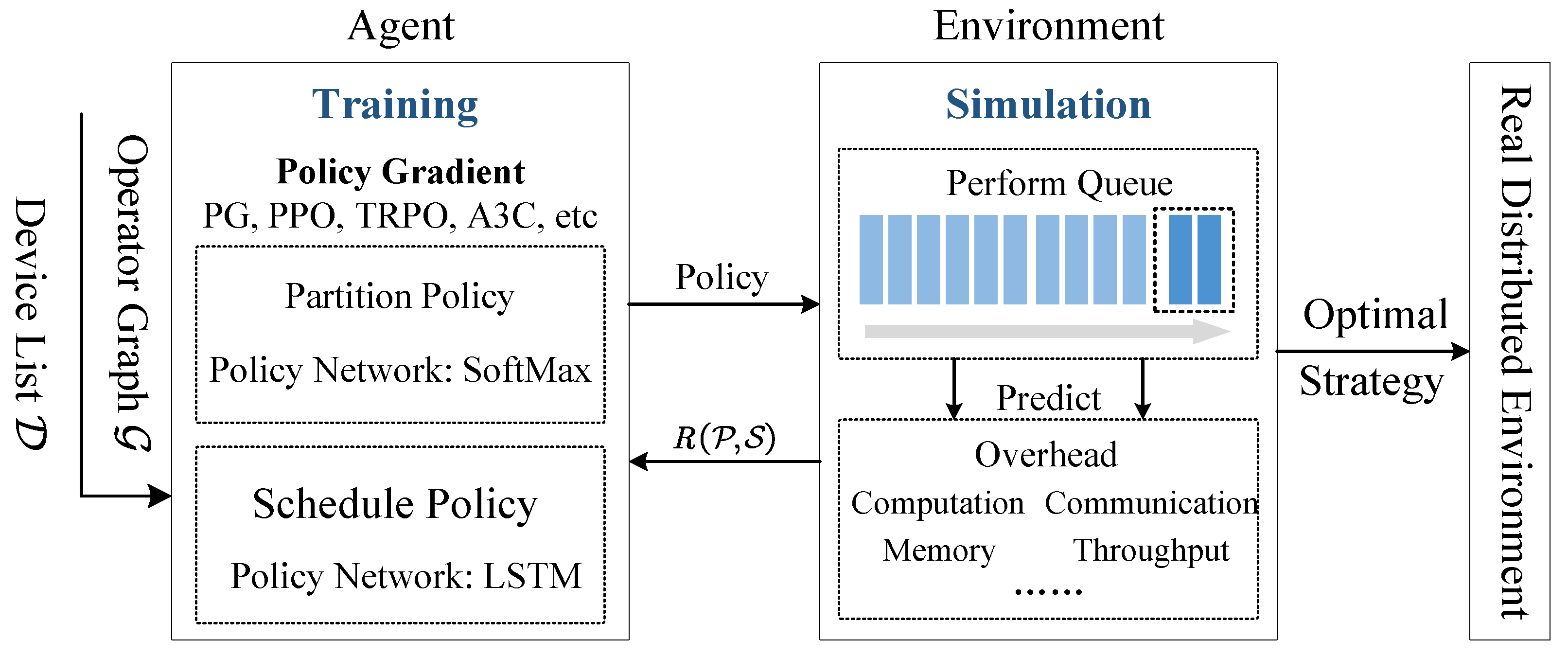
After defining the MDPE model, we introduce the main reinforcement learning model. We will establish a double-layer policy network to generate partition and schedule strategies. To improve the sampling efficiency and algorithm convergence, we introduce proximal policy optimization method, which perform comparably or better than state-of-the-art approaches while being much simpler to implement and tune. The architecture of Trinity is shown in Figure 1.

Trinity is composed of agent and environment. Agent is mainly used for the generation of the model parallel strategy and iterative optimization strategy. Environment consists of a simulator to evaluate the performance of the strategy.

The agent in Figure 1 is the main part of reinforcement learning, which consists of double-layer policy networks: partition network ${\mathcal{N}}_g$ and schedule network ${\mathcal{N}}_s$. Before the strategy search, Trinity takes computational graph $\mathcal{G}$ and device topology diagram $\mathcal{D}$ as input. The agent generates a model parallel strategy through a double-layer policy network. The simulator in environment computes the linear relationship $f(E_i,C_{i,j})$ between computation costs $E_i$ and communication costs $C_{i,j}$, to simulate forward propagation, back propagation, and parameter update. The simulator computes the MDPE model $R({\pi }_g,{\pi }_s)$ according to Formula (8) by collecting performance data, for example, communication costs, computation costs, and memory occupation. Then, environment feeds the reward R back to the agent, and iteratively optimizes the policy network through the proximal policy optimization (PPO) and the above process is repeated until convergence. Finally, the strategy which can maximize the MDPE model $R({\pi }_g,{\pi }_s)$ is executed in the real distributed environment.

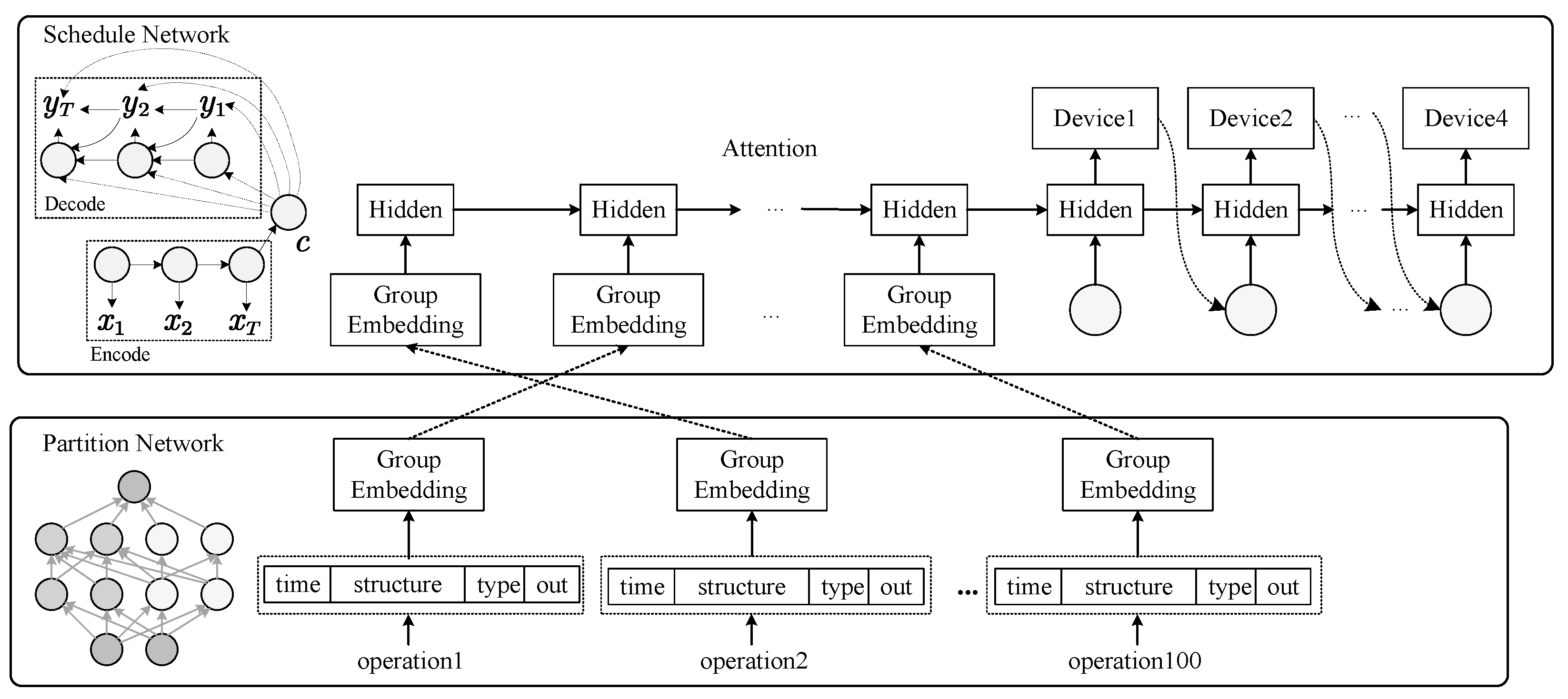
The double-layer policy network architecture of the agent including two networks: namely the partition network used to perform coarse-grained grouping of neural network operators; and the schedule network which generates a schedule policy of groups. The detail is as shown in Figure 2.

4.1.1. Partition Network ${\mathcal{N}}_g$

Partition network ${\mathcal{N}}_g$ is a fully connected network contains two hidden layers of size 64 and 128, and a $30\%$ dropout layer is introduced between them to prevent overfitting. As shown in Figure 2, we embed each operation with four attributes. The following

Table 1. Computational graph feature extraction content.

Feature	Name	Description
time	runtime	The runtime required by the operator, using normalization (Z-score) processing
structure	structure	Using Node2vec to extract graph structure features
type	node type	Building TensorFlow common API vocabulary index
out	output shape	Accumulating the dimensions of all output tensors of the current operator

lists the four parts of the operator features:

• Runtime (time). Designates the runtime of executing the operator on the specified device, in microseconds. To ensure algorithm convergence, standardization (Z-score) processing is performed on the runtime.
• Structure (structure). Use Node2vec to learn and generate graph embedding vectors. Node2vec is a common graph feature extraction method in graph representation learning. It combines the RandomWalk and SkipGram models to learn the co-occurrence relationship between nodes, and generates dense vectors for each node.
• Node type (type). This includes the calculation time of the node, the memory size of the node, and the operator type of the node. We use natural language processing methods; collect 200 commonly used operator words in the TensorFlow API, such as Conv2D, MaxPool, or MalMul; and build a vocabulary, such as Conv2D, MaxPool, or MalMul.
• Output shape (out). Accumulate all output tensor dimensions of the current operator. Accumulate the dimensions of all output tensors of the current operator. For example, if the existing convolution operator outputs a four-dimensional tensor with shape $(2,2,1,64)$, the output shape is $256=2\times 2\times 1\times 64$. The output size of an operator can not only represent the maximum traffic that the operator may generate, but also reflect the memory overhead that the operator may generate.

After the embedding of all operators, the embedding is input to the partition network to generate groups, and the operators in the group are merged into group embedding and output to the schedule network as follows, as shown in

Table 2. Group feature extraction content.

Feature Name	Description
group type	Calculating the mean of all operator types in the group
group outsize	The sum of the output sizes of the operators in the group
relationship between groups	Indicating the connection between groups, and the connection position is set to 1

.

• Group type. Take the average of all operator type embeddings in the group as the first part of the group embedding.
• Group outsize. The output tensor size of all operators in the group is averaged as the second part.
• Relationship Between Groups. This represents the connection relationship between groups. The length of the embedding represents the number of groups (for example, if the operator is divided into 256 groups, the vector length is 256). If an operator in the current group is connected to an operator in the ith group, the ith position of the vector is set to 1, otherwise, it is 0.

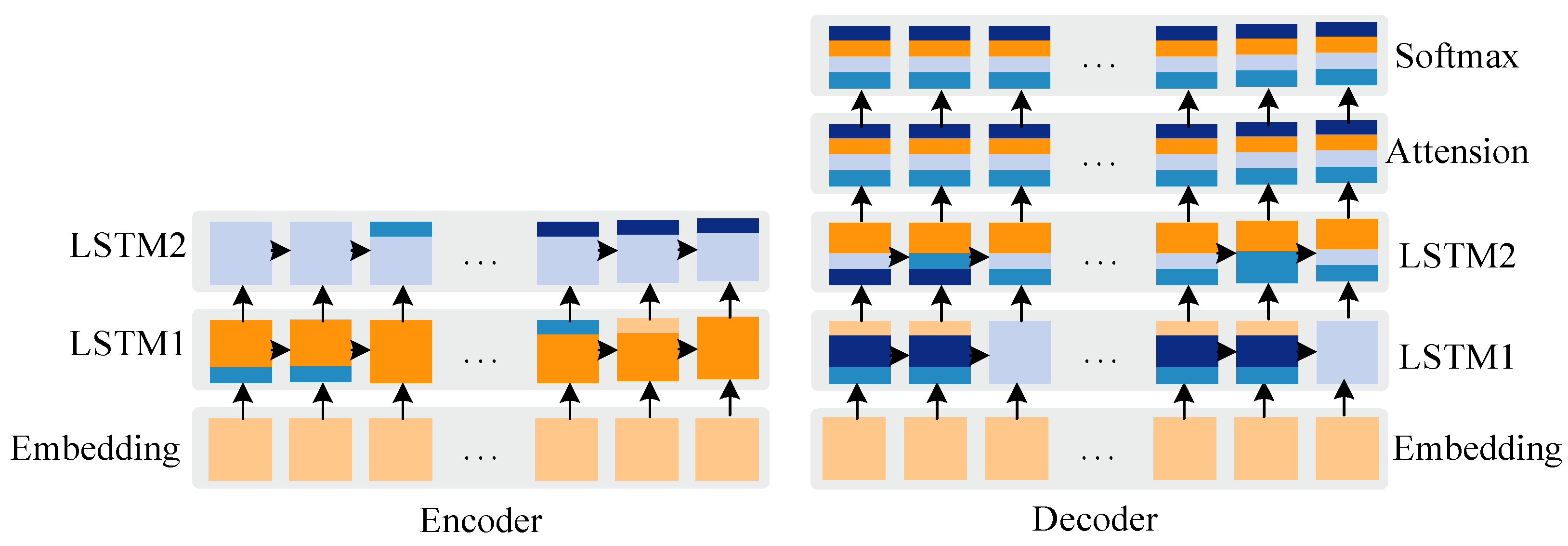
4.1.2. Schedule Network ${\mathcal{N}}_s$

${\mathcal{N}}_s$ is a Seq2Seq network with an attention mechanism and LSTM, and the input and output sequences of variable length are processed through the encoder and the decoder, respectively. As shown in Figure 2, encoder ${\mathcal{N}}_s$ reads the group embedding of $g_i$ at a time and generates k hidden states, where k is a hyperparameter equal to the number of groups.

The decoder obtains a device $d_j$ per prediction and generates an infinite length sequence of the output device. The generated device sequence and the input sequence are in a one-to-one correspondence order, i.e., all operators in the first group will be scheduled to the first device output by the decoder, etc. It is worth noting that each device has a trainable embedding, and the embedding of the previous device will be input to the next decoding prediction.

Moreover, ${\mathcal{N}}_s$ also uses the attention mechanism [13] to pay attention to the state of the encoder. The decoder will sample the device $d_t$ from the softmax layer at step t during the training process. To make the schedule network activation function $u_t$ flatter, we introduce softmax temperature and logarithmic clipping [36], and the activation function $u_t$ can be expressed by the temperature T and the tanh constant C. Therefore, the following methods are used for sampling:   

$$d_t\sim softmax\left(Ctanh\left(u_t/T\right)\right).$$

(9)

Finally, the device sequence output by the decoder is the schedule strategy corresponding to the input packet. The simulator can further simulate the partition and schedule strategy and obtain the reward value through the collaborative optimization $({\mathcal{N}}_g,{\mathcal{N}}_s)$ model.

The iterative optimization of the two-layer policy network requires appropriate and efficient reinforcement learning method. Thus, this paper adopts proximal policy optimization to iteratively optimize the reinforcement learning model.

4.2. Proximal Policy Optimization

Trinity collaboratively optimizes the partition and schedule network using PPO. The goal of PPO is to maximize the expectation of the reward (i.e., MDPE model) and update the policy network parameters.

Therefore, the objective function can be expressed as below:

$$J\left(\pi \right)=J\left({\pi }_g,{\pi }_s\right)=E_{p\left(g,s;\theta \right)}\left(R\right)$$

(10)

Convert expectations to probability distributions, which can also be written as

$$J\left(\pi ;\theta \right)=\sum _{{\pi }_g,{\pi }_s}\left[p\left(g,s;\theta \right)R\right]$$

(11)

The essence of the optimization algorithm is to control the parameters of the policy network and change the probability distribution of the policy to maximize the expected reward. $p\left(g,s;\theta \right)$ represents the probability distribution of the distributed parallel strategy under the given network parameter conditions. R is the reward, which is calculated by the partition strategy g and the schedule strategy s according to MDPE.

The expectation in Formula (10) is approximated by Monte Carlo sampling and iterative optimization using gradient ascent. However, when the parameters are optimized using the gradient, the probability distribution $p\left(g,s;\theta \right)$ will change. Even small parameter changes can cause drastic changes in $p\left(g,s;\theta \right)$, requiring resampling after parameter update. The violent jittering of the probability distribution is also not conducive to algorithm convergence.

Therefore, based on importance sampling, we adopted PPO and rewrote the objective function as the following formula:

$$\underset{p}{max}{\mathbb{E}}_{{\pi }_{old}\sim p_{old}}\left[\frac{p\left(g,s;\theta \right)}{p_{old}\left(g,s;{\theta }_{old}\right)}\left(R-b\right)\right].$$

(12)

$$s.t.KL\left[p_{old}\left(g,s;{\theta }_{old}\right),p\left(g,s;\theta \right)\right]\le ϵ.$$

(13)

where ${\theta }_{old}$ is the vector of policy parameters before the update. We take the probability distribution $p_{old}\left(g,s;{\theta }_{old}\right)$ of the old policy as the proposal distribution and still sample from the old probability distribution. The Formula (13) maintains the difference between $p_{old}$ and p within $ϵ$; b is the mean moving baseline. The optimization problem with constraints can be solved by the conjugate gradient algorithm, but the cost is high.

Let $r_t\left(\theta \right)$ donate the probability ratio $r_t\left(\theta \right)=\frac{p\left(g,s;\theta \right)}{p_{old}\left(g,s;{\theta }_{old}\right)}$. We modify the objective to Formula (14) to penalize $r_t\left(\theta \right)$ for being far from $ϵ$:

$$J_{\theta }=max{\mathbb{E}}_{{\pi }_{old}}\left[r\left(g,s;\theta \right)(R-b),clip\left(r\left(g,s;\theta \right),1-ϵ,1+ϵ\right)(R-b)\right].$$

(14)

where $ϵ$ is a hyperparameter that controls the difference between the old and new distributions, and $clip$ is the truncation function used to truncate the maximum and minimum values of the objective function to ensure that the control always remains between $\left[1-ϵ,1+ϵ\right]$.

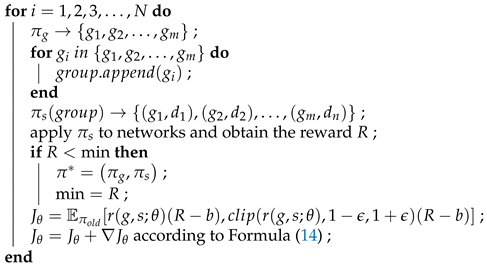
Finally, the objective function is maximized by the stochastic gradient ascent. The complete algorithm execution is shown in Algorithm 1.

Algorithm 1: Parallel policy automatic search algorithm based on PPO.

Data: devices: $\mathcal{D}=\{d_1,d_2,\cdots ,d_n\}$, policy network parameters $\left\{{\theta }_g,{\theta }_s\right\}$

Result: optimal parallel strategy: ${\pi }^{*}$, policy network parameters: $\left\{{\theta }_g^{*},{\theta }_s^{*}\right\}$

Initialization $min\to \infty$ and $R=0$

return ${\pi }^{*}$ and R

In this paper, Adam [37] is used to complete the gradient descent. To reduce the variance, we also introduce a baseline b. If N is the hyperparameter representing the period, then the recursive formula of the exponential moving average reward baseline $EM{A}_N\left(b_n\right)$ is as follows:

$$EM{A}_N\left(b_n\right)=\frac{2b_n+(N-1)EM{A}_N\left(b_{n-1}\right)}{N+1}.$$

(15)

4.3. Simulator

If all the parallel strategies were run in a real distributed environment, a large-scale cluster and considerable time would be needed. Therefore, Trinity introduces a simulator, which can simulate a parallel strategy without relying on real distributed environments.

In the beginning, the parallel strategy will be executed in a real distributed environment to collect the running performance of the model on all devices. Then, the simulator will take over the real distributed environment, and predict the training time by computing the linear relationship between the computation costs $E_i$ and the communication costs $C_i$.

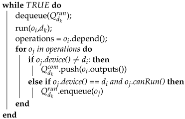
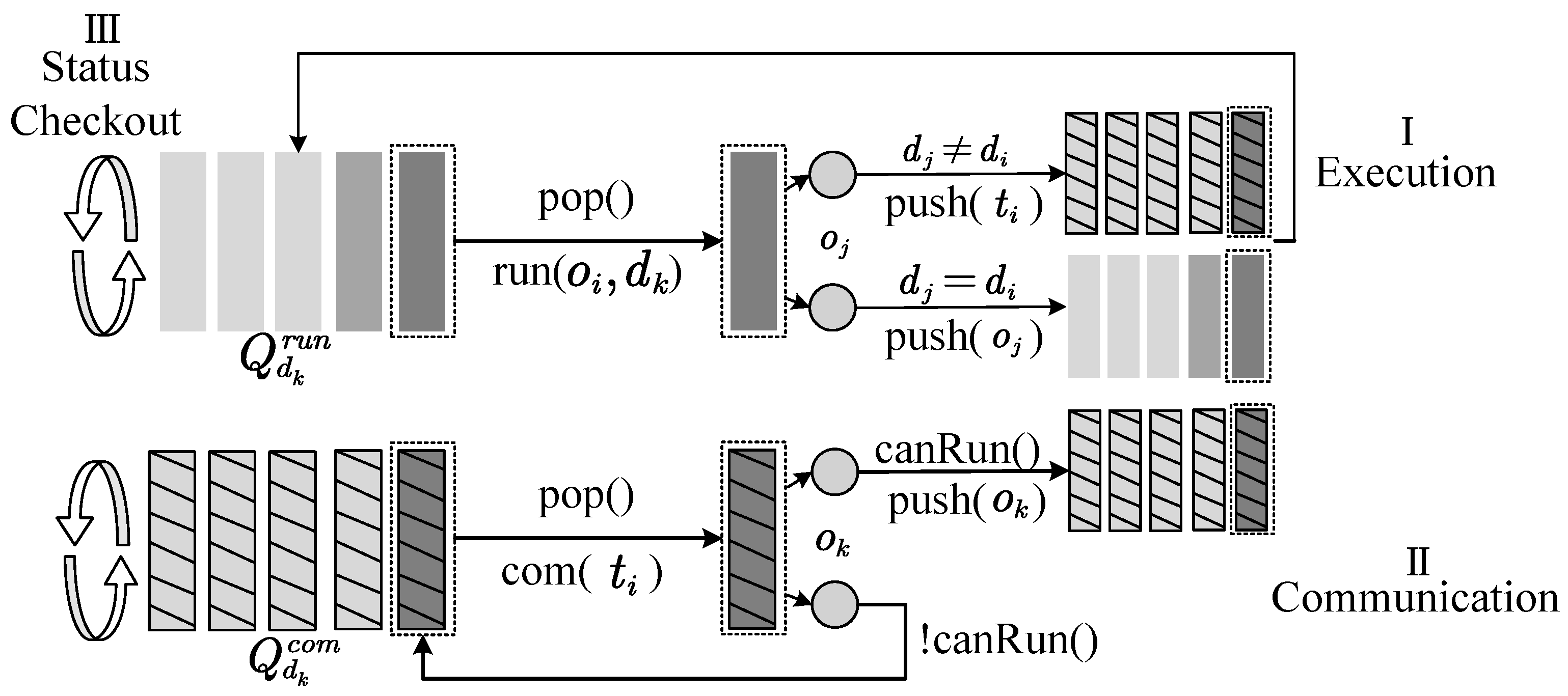
The design of the simulator follows these three principles: (1) per-device d FIFO queues hold runnable operations; (2) communication overlaps with computing; and (3) operators which on the same devices should be executed serially. The simulator workflow is shown in Figure 3.

The simulator maintains two first-in–first-out queues for each device in a dual-threaded manner and generates a time pipeline through a trigger mechanism which mainly includes three key processes: operator execution, tensor communication, and status checking. For the convenience of the explanation, let $Q_d^{\mathit{run}}$ denote the operator execution queue on device d, and record the sequence of operators to be run. Then, let $Q_d^{\mathit{com}}$ denote the tensor queue that will communicate from device d to the other devices. This forms the collection of tensors. The details of the three key processes are as follows.

1. Operator Execution

The operator $o_i$ to be executed from the queue $Q_d^{\mathit{run}}$ is fetched, the operation is completely executed and the output is processed, as the execution in Figure 3I. First, operation $o_i$ is dequeued from the local execution queue $Q_{d_k}^{run}$ to be executed. Second, all operators connected to the operator $o_i$, denoted as $o_j$, are obtained, and the device $d_l$ where node $o_j$ is checked. If $d_j\ne d_i$, the output tensor $t_i$ of $o_i$ is enqueued to $Q_{d_k}^{com}$, and if $d_j=d_i$, whether $o_j$ meets the execution principle is checked, and if it is, it is enqueued to $Q_{d_k}^{run}$. Finally, the status of $Q_{d_k}^{run}$ is checked. If it is empty, trigger the idle state of device $d_k$; and if not, dequeue the next operation from $Q_{d_k}^{run}$ to execute. The detail of operator execution is described in Algorithm 2.

2. Tensor Communication

After tensor $t_i$ communication is completed, other operators that depend on the current tensor are processed, as the execution in Figure 3II. First, dequeue tensor $t_i$ from the communication queue $Q_{d_k}^{com}$ to communicate. Second, obtain all operators $o_k$ that depend on $t_i$, and check whether it is ready to start with the operating principle. If it is ready, put it into queue $Q_{d_k}^{run}$. Finally, judge whether $Q_{d_k}^{com}$ is empty. If it is empty, the communication triggering the state of device $d_k$ is idle. If not, this process is cyclically executed.

3. Status Check

Judge whether $Q_d^{run}$ and $Q_d^{com}$ are empty. If they are empty, the idle state will be triggered; and if they are not empty, they will immediately dequeue to execute the operator execution or conduct tensor communication.   

Algorithm 2: Operator Execution ($o_i$ executes on $d_k$).

Data: $\mathcal{G}(O,E)$, $\mathcal{D}$, $Q_{d_k}^{run}$, $Q_{d_k}^{com}$

Result: None

initialization;

5. Experiment

In this section, we applied Trinity to widely used neural networks in computer vision and natural language processing: InceptionV3, NMT, GNMT, NASNet (large) and PNASNet (large). We measured the performances on the CIFAR10 and PTB datasets and compared the performances with that of Hierarchical proposed by Google.

5.1. Experimental Settings

In this section, we will introduce the experimental settings.

(1) Model. We chose 5 types of deep neural networks widely used in CV and NLP, which are shown in

Table 3. The model and datasets selected for the experiment.

Networks	Operators	Edges	Datasets	Field
InceptionV3	12,745	21,928	CIFAR-10	CV
NASNet-Large	18,644	27,505
PNASNet-Large	14,063	20,718
GNMT	8738	16,564	PTB	NLP
NMT-2layers	16,432	24,235

.

(2) Baseline. We compared the strategy found by Trinity to the following baseline.

Single GPU. We executed the model on a single GPU. Neural networks usually run fast on a single GPU because they incur no cross-device communication cost. Thus, a single GPU is an important baseline. However, a single GPU cannot afford the training of larger networks.

Layered Expert. We used different parallel strategies for different models. For InceptionV3, we trained it on a single device because it is difficult to achieve parallel operations with high communication performance for this method. For the 2-layer NMT, we scheduled each LSTM layer to different devices and bind the attention mechanism and softmax layer to the same device. We divided NASNet into different layers, including NASNet-Large and PNASNet-Large.

Hierarchical. Google proposed a hierarchical method using reinforcement learning to search for the best placement of operators based on a 2-layer policy network. However, this method only considers the single optimization aspect of runtime and the cost of this method is high.

(3) Environment of experiments. We performed experiments on a single cluster, including a genuine Intel CPU with 12 GB of memory and 4 NVIDIA Tesla P100 high-performance GPU with 11 GB of memory and a bandwidth of 28 MB/s (Santa Clara, CA, USA). The software configuration is shown as below:

The operating version is Ubuntu 18.04.4 LTS (Canonical Ltd., London, UK), Linux kernel version is Linux 4.15.0-123-generic, GPU version is NVIDIA Tesla P100, CUDA version is CUDA10.1.243 (NVIDIA) and TensorFlow version is TensorFlow1.15.0 (Google Brain Team, Mountain View, CA, USA).

(4) Algorithm Configuration. The partition policy network ${\mathcal{N}}_g$ uses a feed forward neural network with softmax, which contains two hidden layers with sizes of 64 and 128. The softmax output size is set to be equal to the number of groups, and both are 256. For the schedule policy network ${\mathcal{N}}_s$ two-layer LSTM, the size of the hidden layer is set to 256, and the softmax output size was set to 2, 4, or 8 equal to the number of devices.

5.2. Comparison of Experimental Results

In the experiment, Adam is used to collaboratively optimize the partition and schedule policy networks. We use the gradient clipping method with a learning rate of $0.1$ and a norm of $1.0$, where the constant of tanh is set to $C=5.0$ and temperature $T=10.0$. To prevent falling into local minimum and encourage more exploration, we add noise to the logits of the policy networks in the first 500 training steps, and the maximum noise is $0.1$. For the reward, the MDPE model is adopted, and the hyperparameters are set as follows: $\alpha =0.5$, $\beta =0.3$, and $\gamma =0.2$. User tolerance $\widehat{C}$ and $\widehat{M}$ are both set to 8. We give recommended values for the hyperparameters in this paper based on the experiments and communication of some industry experts.

5.3. Strategy Visualization

In this section, we take the NMT model as an example. We will display the best parallel strategy searched by Trinity on 4 GPUs clusters. Figure 4 shows the fine-grained partition of the NMT model by Trinity. Compared with the Layered Expert, Trinity has a finer-grained division of the LSTM layer, attention layer and softmax layer. This is not possible for expert design: it colocates all operations in a step. Compared with Hierarchical, the partition and schedule strategy of Trinity is generally similar to Hierarchical, but Trinity groups the LSTM operations in the decoder more intensively, and tends to trade part of the memory overhead for the optimization of the communication cost.

Experiments show that the Trinity method supports the fine-grained division of neural network layers and has the ability to trade off computation and communication overhead. In Figure 4, different colors in the figure represent different GPUs. We find the following: (1) embedding is a typical parameter-intensive submodel. The results show that Trinity is suitable for embedding to use memory or storage in exchange for computing and communication resources; (2) The LSTM is a computationally intensive operation. Trinity seeks to divide the LSTM layer more flexibly and achieves load balancing by weighing the computation and communication costs. Attention and softmax both have parameter and computation intensiveness, i.e., dual intensiveness. Trinity implements partition and schedule costs for attention and softmax from multiple dimensions, to reduce the parameter synchronization while ensuring load balancing. The parallel strategy of the layered NMT network model shown in Figure 4 takes only $2.56$ s to execute forward propagation, backpropagation, and gradient computation.

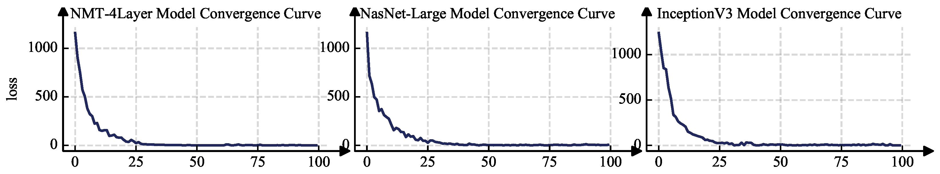
Figure 5 shows the convergence curves of the Trinity algorithm based on NMT, NASNet, and InceptionV3. We proved the convergence and effectiveness of this method. It is worth noting that, in this experiment, we used the standard Adam method to implement the gradient descent algorithm. No noise is introduced in the initial stage of training, and only the standard Adam method is used to implement the gradient descent algorithm. The total number of iterations $step=100$. We recorded the loss value for each iteration. It can be seen from the curve that the algorithm continues to converge. The results show that, whether for the NLP network (NMT) or CV network (InceptionV3 and NASNet), it only takes approximately 25 rounds of iterations for the loss of the reinforcement learning search algorithm to drop to less than 10.

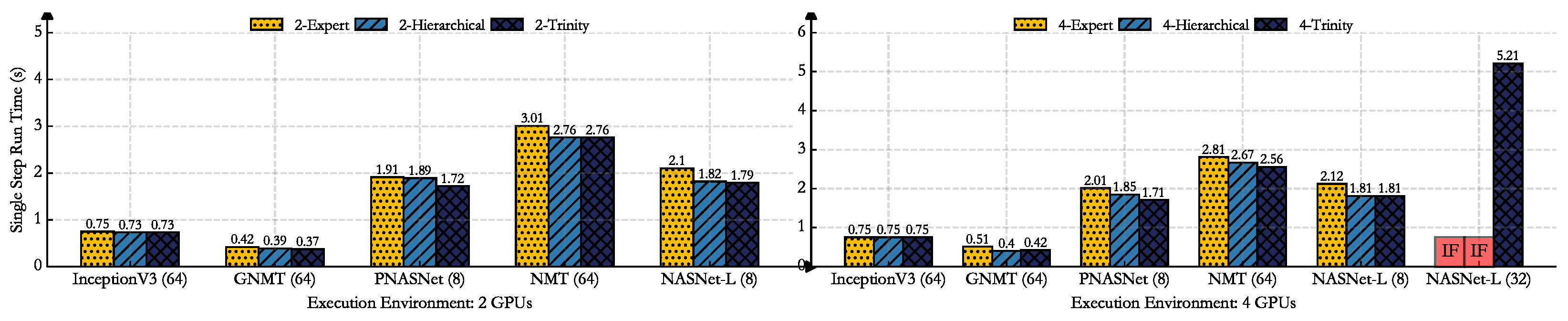
5.4. Strategy Performance Analysis

In this section, we will compare the performance of Trinity with other baselines from different perspectives including runtime, peak communication, peak memory, and search time. Our experiment uses the CIFAR-10 and PTB datasets and tests the Inception, NMT, NASNet (large), and PNASNet (large) models.

The experimental results are shown in Figure 6, Figure 7 and Figure 8 and

Table 4. Performance comparison of Trinity and parallel strategies of different models.

	Runtime(s)	Numbe	Runtime(s)	Runtime/PeakCommunication/Memory
Network	GPU	GPUS	Expert	Hierarchical			Trinity
InceptionV3 (64)	OOM	2	0.75	0.73	6.0	5.8	0.73	5.6	5.3
		4	0.75	0.75	7.8	6.0	0.75	7.9	3.4
GNMT 2layer (64)	0.30	2	0.42	0.39	1.2	2.1	0.37	1.0	2.5
		4	0.51	0.40	1.8	0.9	0.42	1.9	1.1
NMT 2layer (64)	OOM	2	2.76	3.01	9.1	6.9	2.76	7.1	7.2
		4	2.81	2.67	5.9	8.7	2.60	4.4	8.8
NASNet-L (8)	OOM	2	2.10	1.82	6.9	4.6	1.79	6.1	3.7
		4	2.12	1.81	7.3	4.0	1.81	7.2	3.9
NASNet-L (32)		4	OOM	OOM			5.21	12.2	11.3
PNASNet-L (8)	1.45	2	1.91	1.90	3.8	6.3	1.70	3.3	6.3
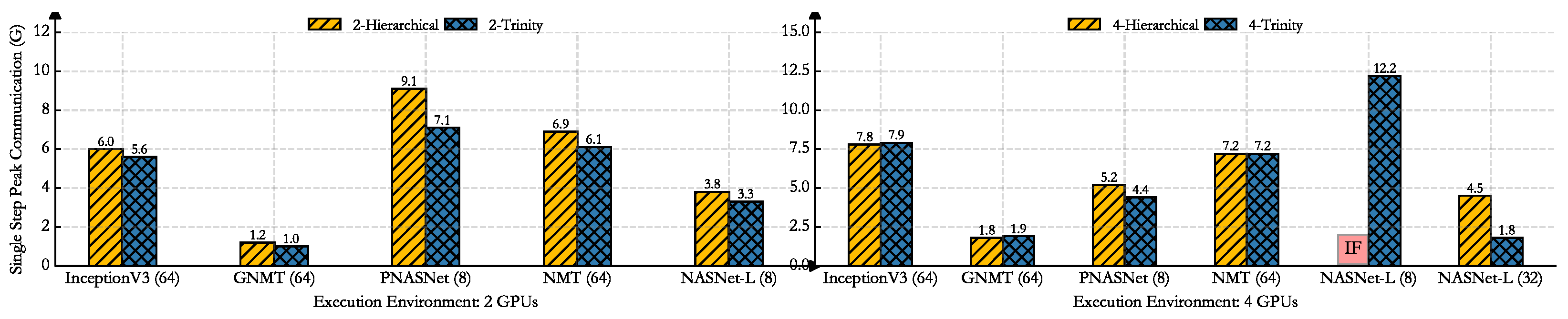
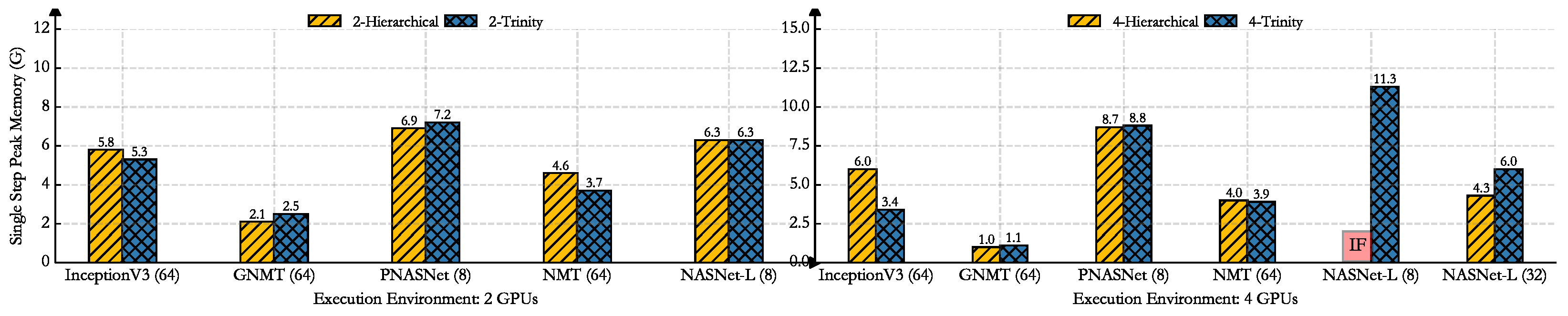
		4	2.01	1.85	4.5	4.3	1.71	1.8	6.0

below. We show the performance comparison with Trinity and GPU only, layered expert, and Hierarchical from three dimensions: (1) runtime: the model completes a single forward propagation and derivation; (2) peak communication: the maximum communication cost among all hardware devices; (3) peak memory: the maximum memory occupation among all hardware devices. In the legend of Figure 6, Figure 7 and Figure 8, the numbers (2 or 4) represent the number of GPUs. Expert, Hierarchical and Trinity are the baseline and the method proposed in this paper, respectively. Single step means that the model completes a single forward propagation and derivation.

Compared with Google’s Hierarchical, the InceptionV3, and GNMT networks, the runtime of the parallel strategy searched by Trinity is similar, but it has a better performance in communication and memory. For large-scale networks, such as NASNet-L and PNASNet-L, Trinity has a better balance of performance. It is worth noting that the Hierarchical method cannot search for a suitable model parallel strategy for NASNET-L based on 4 GPU, but Trinity can. It only takes 5.21 s to execute the parallel strategy. Trinity has less runtime than layered expert methods.

To be clear, a single GPU is the strongest baseline, which incur no cross-device communication cost. Model parallelism is suitable for scenarios in which the AI model scale is too large and cannot be trained on a single GPU. So, Trinity and single GPU training are applicable to different scenarios. Trinity is not trying to surpass, but hopes to be closer to the runtime under a single GPU.

We compute the improvement of the performance indicators compared with Hierarchical in

Table 5. The comparison of the parallel performance improvement rate and search time.

		Search Time (1000 Iterations)		Percentage Decrease
Network	GPUS	Hierarchical	Trinity	Runtime	Communication	Memory	Search Time
InceptionV3 (64)	2	1.2 K	0.7 K	0.0%	6.8%	8.6%	41.7%
	4	3.6 K	2.0 K	0.0%	−0.8%	43.4%	44.4%
GNMT 2layer (64)	2	18.9 K	8.9 K	5.1%	16.1%	−18.8%	52.9%
	4	20.6 K	9.8 K	−5.0%	−7.1%	−14.6%	52.4%
NMT 2-layers (64)	2	27.8 K	10.3 K	8.3%	20.9%	−4.5%	62.9%
	4	30.5 K	17.1 K	4.1%	14.7%	−0.3%	43.9%
NasNet-L (8)	2	12.5 K	9.8 K	1.6%	12.5%	20.0%	21.6%
	4	12.6 K	9.1 K	0.0%	1.6%	2.7%	27.8%
NasNet-L (32)	4	21.6 K	16.6 K	-	-	-	23.1%
PNasNet-L (8)	2	18.6 K	18.7 K	9.0%	13.8%	0.0%	−0.5%
	4	28.8 K	20.1 K	7.6%	60.2%	−40.0%	30.2%

and compare the time required for the Hierarchical and Trinity methods in the case of 100 search iterations. The table analysis shows that the trinity will exchange part of the memory overhead for communication optimization. The overall performance is more balanced, and the runtime is also reduced to varying degrees.

Due to the introduction of the execution simulator in Trinity, it can achieve up to a 40% increase in parallel strategy search speeds, in most cases. It can be proven that the introduction of the execution simulator can greatly reduce the time required for search and sampling. Although Trinity introduces a simulator to simulate the execution process, the performance evaluation using these experimental data is performed in a real distributed environment.

5.5. Simulator Performance Analysis

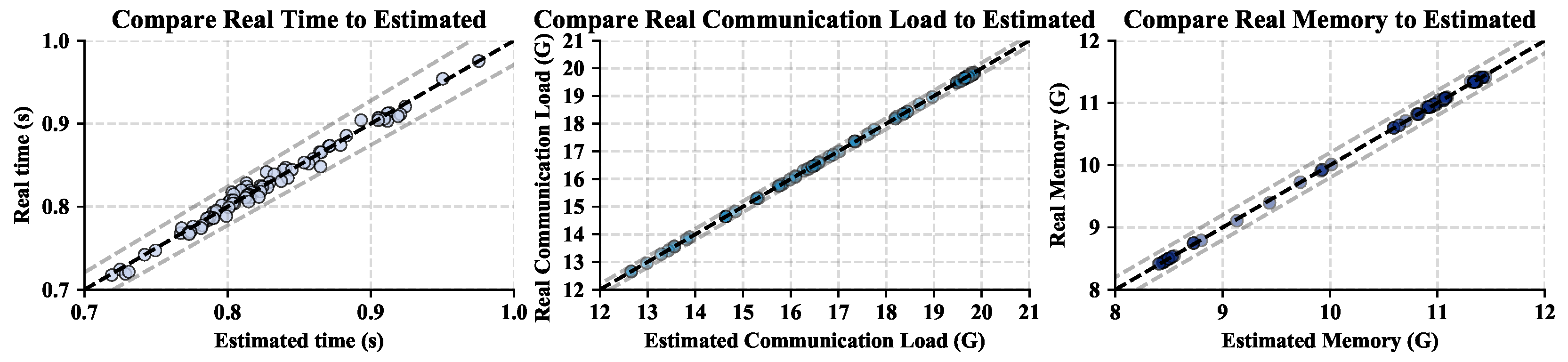
To verify the effectiveness of the simulation accuracy of the simulator for the reinforcement learning algorithm, this paper takes InceptionV3 as an example and plots the real operating performance and simulated operating performance under different strategies in Figure 9. As shown in Figure 5, the abscissa represents the simulated operating performance, and the ordinate represents the true distribution. The operating performance of the environment is measured from left to right as follows: runtime, communication load, and memory load. The left figure compares the runtime error, and the simulated error interval is approximately ±0.05 s. The middle picture compares the peak communication error, and the simulated error interval is approximately ±0.4 GB. The right picture compares the peak memory error, and the simulated error interval is approximately ±0.4 GB. The experiments prove that the simulator has a reasonable range of errors during operation, communication, and memory, which has little effect on reinforcement learning training.

Furthermore, compared with the real distributed environment, the simulator increases the parallel strategy search speeds up to 40% on average.

6. Conclusions

This paper addresses on the problem of the poor performance of model parallel training caused by a single optimization aspect, and proposes the Trinity method, which uses reinforcement learning to achieve the automatic search and tuning of parallel algorithms for large-scale complex neural network models. Furthermore, this paper constructs a three-dimensional collaborative optimization evaluation model to guide reinforcement learning iterative optimization, and improves the comprehensive performance in terms of the runtime, communication load and memory consumption. A simulator is also introduced to improve the sampling efficiency and accelerate the policy search time. Our experiments use CIFAR10 and PTB datasets based on Inception, NMT, NASNet (large) and PNASNet (large) models. The result shows that, compared with the hierarchical method, Trinity can achieve the performance load balancing with less memory overhead in exchange for performing the optimization of runtime and communication costs.