Article

Skeptical Learning—An Algorithm and a Platform for Dealing with Mislabeling in Personal Context Recognition

Department of Information Engineering and Computer Science, University of Trento, 38123 Trento, Italy
*
Author to whom correspondence should be addressed.
Algorithms 2022, 15(4), 109; https://doi.org/10.3390/a15040109
Submission received: 24 January 2022 / Revised: 9 March 2022 / Accepted: 22 March 2022 / Published: 24 March 2022

Abstract

:
Mobile Crowd Sensing (MCS) is a novel IoT paradigm where sensor data, as collected by the user’s mobile devices, are integrated with user-generated content, e.g., annotations, self-reports, or images. While providing many advantages, the human involvement also brings big challenges, where the most critical is possibly the poor quality of human-provided content, most often due to the inaccurate input from non-expert users. In this paper, we propose Skeptical Learning, an interactive machine learning algorithm where the machine checks the quality of the user feedback and tries to fix it when a problem arises. In this context, the user feedback consists of answers to machine generated questions, at times defined by the machine. The main idea is to integrate three core elements, which are (i) sensor data, (ii) user answers, and (iii) existing prior knowledge of the world, and to enable a second round of validation with the user any time these three types of information jointly generate an inconsistency. The proposed solution is evaluated in a project focusing on a university student life scenario. The main goal of the project is to recognize the locations and transportation modes of the students. The results highlight an unexpectedly high pervasiveness of user mistakes in the university students life project. The results also shows the advantages provided by Skeptical Learning in dealing with the mislabeling issues in an interactive way and improving the prediction performance.

1. Introduction

In recent years, with the fast paced development of mobile devices, Mobile Crowd Sensing (MCS) has become an emerging sensing paradigm where, as from [1], ordinary citizens contribute data sensed or generated from their mobile devices. Such data are then aggregated for crowd intelligence extraction and people-centric service delivery. Human involvement is one of the most important characteristics of MCS, especially in applications where participatory sensing applies. One such example is the applications that are designed for environmental monitoring. The work in [2] applies the MCS-RF model to infer the real-time and fine-grained PM2.5 throughout Beijing. In their application, users can upload images with a time stamp and GPS information. The users’ input is used along with other official data sources, such as meteorological data and traffic data published by relevant agencies to carry out the environmental monitoring. Another kind of application are those designed to monitor the user’s health status. The TrackYourTinnitus (TYT) project tracks the user’s tinnitus by their answers to questionnaires and the sensor data collected by their phone. Similarly, TrackYourHearing (TYH), TrackYourDiabetes (TYD), and TrackYourStress (TYS) keep track of the progress of users’ hearing loss, diabetes, or stress level, respectively [3]. This helps the users to be more aware of symptom changes in specific contexts. Finally, there are other applications that collect urban data, such as the reports of damaged infrastructures, with the final goal of monitoring urban safety [4,5]. In this case, the user is asked to report observations by answering questionnaires or uploading images.
These examples above are just some among many MCS applications that collect both the sensor data generated by the mobile phone and the subjective data generated by users. However, normal (non-expert) users might provide an incorrect report or annotations due to the users’ response biases, cognitive bias, carelessness [6,7], and even malicious behavior. Moreover, these MCS systems cannot detect whether the information given by the users are correct or not, while the correctness of the user’s input is important to the MCS applications or systems, especially the ones that using machine learning algorithms in the back-end. This is because most of the existing MCS applications do not have access to the knowledge.
We propose Skeptical Learning, which is a platform running an interactive learning algorithm to detect the user’s incorrectness and to deal with the mislabeling issues. The key idea is that the machine is enabled to use available knowledge to check the correctness of its own prediction and of the label provided by the user. The machine is trained with the user’s label and the sensor data collected from the user’s phone. Meanwhile, by keeping track of the sequence of wrong and right answers, the machine builds a measure of confidence towards itself and towards the user. When the machine detects that the user’s input is not compatible with its prediction and the machine is confident enough, it will challenge the user by sending another question to them to obtain a confirmed input. This interactive learning strategy will help to improve the quality of the user’s input and, hence, to improve the machine learning performance. In this context, by available knowledge, we mean both the knowledge inductively built out of the previous learning activity and the knowledge that may come from third parties or may be built-in as a priori knowledge. In particular, the prior knowledge is used to perform Description Logic (DL) reasoning [8] over the known facts, as they are expressed in a language with no negations and no disjunctions.
The two main contributions of this work are:
  • An algorithm for Skeptical Learning (SkeL), which interacts with the user and challenges him/her when his/her feedback is not consistent with what it has learned about the world. The key component is an algorithm for managing conflicts that uses a confidence measure applied to both humans and machines;
  • A general MCS platform for integrating, at scale, sensor data and user’s generated data in the form of labels, together with the static knowledge of the world. The former informs SkeL about the world evolution whereas the latter codifies the prior knowledge, which is used in the conflict resolution phase.
The algorithm and platform have been tested and evaluated as part of a long-term series of experiments aimed at studying the university student life in various campuses worldwide. In this setting, users are asked to provide feedback about their situational context, thus acquiring information about their personal activities, as well as the surroundings. Since the beginning, it was clear that a certain percentage of the annotation labels provided by students would be somewhat unreliable. As detailed in the evaluation section, this percentage turned out to be very high, and much higher than originally expected. This fact, plus the fact that the validation results show that SkeL substantially improves over an approach relying only on the noise-robustness of the underlying learning algorithm, provides evidence of the work described in this paper. This paper describes SkeL and the platform in their final form. A preliminary version of the main SkeL algorithm was used and described in [9,10], where the main goal was to understand the student mislabeling behavior. With respect to this earlier work, the main novelties are: (1) the MCS architecture and application are completely novel, (2) the SkeL algorithm has evolved substantially with the predictor now implemented as a hierarchy of classifiers matching the prior knowledge, and, finally, (3) the experiments and evaluation have been substantially extended by comparing our algorithm with three alternative strategies for dealing with conflicts.
The remainder of this paper is organized as follows. In Section 2, we describe the SkeL main algorithm and most important components. In particular, in Section 2.1, we shortly describe the organization of the prior knowledge; in Section 2.2 we introduce the main algorithm; in Section 2.3 we describe the prediction algorithm, whereas, finally, in Section 2.4, we specify the algorithm that manages the conflicts between the human and the machine. Next, in Section 3, we introduce the MCS platform. This section is organized in three parts: the main functionalities of the front-end (Section 3.1), of the back-end (Section 3.2), and how the data are organized in the storage (Section 3.3). Section 4 describes the experiments inside which SkeL and the platform have been evaluated. Section 5 describes the evaluation that is focused on the pervasiveness of the user mistakes (Section 5.1) and of the performance of the machine learning algorithm (Section 5.2). Finally, we close with the related work and conclusions, respectively, in Section 6 and Section 7.

2. The Skeptical Learning Algorithm

Figure 1 depicts a high-level view of the functionalities of the SkeL main algorithm, as presented in Algorithm 1. On the right side, a set of n sensors S 1 , , S n sense the world and produce a set of streams { x t } S i , where x t is the value collected by the sensor S i at time t. The function sensorReading generates X t , which represents the set of all of the sensor data streams at time t. On the left side, the user is asked to provide a label y t as his/her annotation to a certain property P j at time t. The function askUser generates the stream of labels Y t . All these functionalities are implemented as an APP, called i-Log [11], which can be downloaded from the PlayStore. The sensor data and user’s labels are used to train a machine learning predictor PRED. PRED consists of a repertoire of m learning algorithms f 1 , , f m , each taking a stream of data x t as an input and producing a score f k ( x t , y ) for the labels, which are possible values of a certain property P j . Similarly to the user, PRED provides its internally predicted labels Y ^ .
Both the user’s label y t and the predictor’s label y ^ t are used by SkeL during the comparison phase. We can also see y t as the user’s perception of the world, whereas y ^ t is the prediction generated by the machine with the knowledge learned so far from data. The conflict between the two labels happens when the predictor is not trained enough or the user provides an incorrect label. The main idea of SkeL is to check the correctness of the predicted label and the user’s annotation by leveraging its prior knowledge. This step is carried out by the function solveConflict. This function first checks whether the two labels are compatible and, when a conflict arises, two situations are possible. The first one is when the predictor has low confidence. In this situation, the user’s label is selected and the predictor is retrained with the new data. The second situation is when the predictor’s confidence is high enough: solveConflict calls function challengeUser to have another round of the interaction by asking again for the user’s annotation. As we are assuming a collaborative rather than adversarial user, his/her second annotation y * is taken as the correct label and added to the training set to retrain the predictor. The predictor can improve its performance after rounds of training.
Algorithm 1 Skeptical Learning (SkeL)
1:
procedure SkeL( θ )
2:
      init c u = 1 , c p = 0
3:
      while trainMode( c p , c u , θ ) do
4:
           x t = SENSOR R EADING ( )
5:
           y t = ASK U SER ( )
6:
           y ^ t = P RED ( x t )
7:
          train ( x t , y t )
8:
          update ( c p , y ^ t , y t )
9:
      while refineMode( c p , c u , θ ) do
10:
           x t = SENSOR R EADING ( )
11:
           y t = ASK U SER ( )
12:
           y ^ t = P RED ( x t )
13:
          solveConflict ( c p , c u , x t , y ^ t , y t )
14:
      while True do
15:
           x t = SENSOR R EADING ( )
16:
           y ^ t = P RED ( x t )
17:
          if  min y ^ t SM ERS ( y ^ t ) C ONF ( x t , y ^ t , c y ^ t p ) θ  then
18:
              y t = ASK U SER ( )
19:
             solveConflict ( c p , c u , x t , y ^ t , y t )
The following subsections provide a detailed view of the main components implemented in the back-end.

2.1. The Prior Knowledge

To integrate the user labels and the predictor labels, we exploit a knowledge component called SK, for Schematic Knowledge, containing general prior knowledge about the world (see Figure 1). As described in detail below, SK is exploited during conflict resolution (see Figure 1). A detailed description of SK is outside the main focus of this paper; the interested reader can read [12] for a detailed account of the approach and the resource.
Here, it is worth noting that SK is a hierarchy; more precisely, it is a multi-rooted DAG, where each node is labeled with a concept and where a child–parent link codifies a subsumption axiom between a more specific and a more general concept. This hierarchy has more than 100 thousand nodes and codifies a few million subsumption axioms. One trivial example of SK content is a subsumption axiom stating that vehicle is a more general concept than bus: in DL formulas, b u s v e h i c l e . Another example is any general statement about locations and sub-locations; for instance, the fact that department buildings are always inside (they are partOf) the university premises. The hierarchy in Figure 2, which has been exploited in the evaluation, is a very minor portion of the SK hierarchy itself.
From a technical point of view, it is worth noting how the hierarchy in Figure 2 is (partially) a part Of hierarchy rather than an is-a hierarchy, the latter being directly codified into a set of subsumption axioms. PartOf relations on locations can be codified as subsumption relations by seeing locations as sets of points. Under this assumption, the points in a part are always a subset of the points in the whole. The SK encompasses both isa-like and partOf-like relations (the first being called hyponym, the second, meronym) [12].

2.2. The Main Algorithm

The pseudocode of SkeL is reported in Algorithm 1. To keep the description simple, and without a loss of generality, we assume below that there is a single property of interest P, e.g., the location or the transportation means of the user at a certain time. We represent by Y the set of possible values for this property. SkeL can be in one of three modalities that, for simplicity, we assume are activated sequentially, namely: Train mode performed in usual supervised learning, Refine mode, where it checks the quality of the user answers and, under certain conditions, it challenges them, and the Regime mode, where it starts being autonomous and only queries the user for particularly ambiguous instances.
The algorithm takes as an input a confidence threshold θ . It starts by initializing the user confidence c u to one and the predictor confidence c p to zero for all classes ( | c u | = | c p | = | Y | ). Then, the training phase begins. The algorithm collects sensor readings ( x t ) to be used as an input for the predictor. The system then asks the user for a label ( y t ), with the goal of using it as ground truth. The input–output pair trains the predictor by following the train procedure. This can be carried out either via batch learning (where the predictor is retrained from scratch) or via an online learning step [13], where the new input–output pair is used to refine the current predictor. The choice between these learning modalities depends on the specific implementation and constraints, e.g., the storage capacity; see the experiment described below. After training, the confidence of the predictor is modified via the update procedure, which takes as an input the ground truth label and the one predicted before the training step. The update procedure takes as an input a confidence vector, a tentative label ( y ^ t ), and a ground truth label ( y t ), and updates the confidence vector according to the relationship between the two labels. The new confidence vector computed is as a label-wise running average accuracy over the current and past predictions, for a certain window size d. Notice that the confidence updates are applied not only to the predicted and ground truth label pair, but also to all implied label pairs according to the SK, i.e., those from the root to the predicted (respectively) ground truth label.
The training stage stops when the system is confident enough to challenge the user label. Equation (1) shows the computation of the confidence in a prediction label y. c y p is the confidence that the predictor has in label y. Since the predictor is implemented as a set of classifiers matching the hierarchy shown in Figure 2 (the details of the predictor will be introduced in the next section), we use function f PARENT ( y ) ( x , y ) to present the score of the prediction label y generated by the classifier on y’s parent node.
C ONF ( x , y , c y p ) : = c y p · f PARENT ( y ) ( x , y )
when a predicted label is compared with a user-provided label, care must be taken in making a sensible comparison. If the two labels belong to different branches of the hierarchy (e.g., Train and On foot in Figure 2), they cannot be directly compared, as confidences are normalized across siblings. Therefore, the system recovers all of the labels in the hierarchy up to the first common root, i.e., the least common subsumer [8], and compares them instead of the original ones. Thus, for instance, in the previous example, Train implies In vehicle, which is then compared to On foot, as they are both children of On the move.
The system stays in training mode until the expected probability of contradicting the user becomes bigger than the threshold:
TRAIN M ODE ( c p , c u , θ ) : = E [ 1 1 ( C ONF ( x , y ^ , c y ^ p ) > c y u · θ ) ] θ
where 1 1 ( φ ) evaluates to one if φ is true and zero otherwise, and the expectation is taken over all inputs seen so far. The E [ 1 1 ( φ ) ] is the expected probability of the zero and one list generated by 1 1 ( φ ) . The labels to be compared are obtained as ( y ^ , y ) = LCS _ C HILDREN ( P RED ( x ) , y u ) , where P RED ( x ) , the predicted label for input x , y u is the label provided by the user for that input, and the LCS _ C HILDREN procedure outputs a pair of implied predicted/user labels, which are children of the least common subsumer (see Section 2.3 for more details about this procedure). The user is contradicted when the confidence in the predicted label exceeds a factor θ of the confidence of the user in his/her own label.
When it enters into refine mode, the system keeps asking the user for labels while comparing them with its own predictions. solveConflict manages this comparison and its consequences, as described below. This refinement phase ends when the predictor is confident enough and stops asking for user feedback for every input, and selectively queries the user on those labels that are highly “difficult” to decide upon. In the general, production level of the system, it will be the user who decides when to switch modes, thus there is a trade-off between the system maturity and cognitive load. A simple fully automated option, similar to the one used for the train mode, consists of staying in refine mode as long as the expected probability of querying the user exceeds the threshold:
REFINE M ODE ( c p , c u , θ ) : = E [ 1 1 ( C ONF ( x , y ^ , c y ^ p ) θ ) ] θ
again, with the expectation taken over all inputs seen so far. Note that, given that the system has no access to the user label here, it takes a conservative approach and considers the smallest confidence among the ones of the subsumers (SMers) of its (leaf) prediction; see line 17 in Algorithm 1.
After leaving the refine mode, the system enters the regime, where it stays indefinitely. While in regime mode, the system stops asking feedback for all inputs and starts an active learning strategy [14]. In particular, it will query the user only if the confidence computed for a certain prediction is below the “safety” threshold θ . When it decides to query the user, the system includes the tentative label in the query, and then behaves as in refinement mode, calling solveConflict to deal with the comparison between the predicted and the user labels.

2.3. The Predictor

The prediction procedure PRED is implemented as a hierarchy of classifiers matching the SK ontology for the property to be predicted. There is one multiclass classifier for each internal node in the ontology (bold contour nodes in Figure 2), discriminating between its children. The prediction starts from the root classifier and progresses down in the hierarchy following the highest scoring class at each node, until a leaf node is reached, which is the class that is eventually predicted. In the first iteration, when no training has been performed yet, each classifier returns a random label. See Algorithm 2 for the pseudocode of Pred, where f y ( x , y ) is the classifier at node y and y r o o t is the most general value for the property (e.g., a generic Location in Figure 2). The input of the predictor algorithm is the sensor data.
Algorithm 2 Hierarchical predictor
1:
procedure Pred( x )
2:
      init y = y r o o t
3:
      while  n o t IS _ LEAF ( y )  do
4:
           y = argmax y children ( y ) f y ( x , y )
5:
      return y
Note that, thanks to the fact that the transitive closure over the SK axioms is pre-computed, the system can infer, at run time, all of the labels that subsume those provided by the user, i.e., all those from the root to the user label. Each classifier in the path is thus retrained with the addition of its corresponding input–output pair during a train procedure.

2.4. The Conflict Management Algorithm

The solveConflict procedure is described in Algorithm 3. solveConflict takes as an input the predictor and the user confidence vectors c p and c u , the input x with its predicted label ( y ^ ), and the label given by the user (y). The first step is to compare the two labels according to the isCompatible procedure. As the SK encodes a subsumption hierarchy for the property of interest, the procedure returns as true if the two labels are the same or if one subsumes the other. When the two labels are compatible, a consensus label is taken as the ground truth, and the predictor and user confidences are updated accordingly. As a natural choice for the consensus, the system chooses the more general among the two labels, this being the choice also used in the experiments. The motivation is that both the user and the system are taken to be truthful and, therefore, the system chooses the label that carries more meaning.
Algorithm 3 Procedure for solving labeling conflicts
1:
procedure solveConflict( c p , c u , x , y ^ , y )
2:
      if isCompatible ( y ^ , y )  then
3:
           y * = CONSENSUS ( y ^ , y )
4:
          update ( c p , y ^ , y * )
5:
          update ( c u , y , y * )
6:
      else
7:
           ( y ^ , y ) = LCS _ C HILDREN ( y ^ , y )
8:
          if Conf( x , y ^ , c y ^ p ) c y u · θ  then
9:
              train ( f , x , y )
10:
             update ( c p , y ^ , y )
11:
          else
12:
              y * = CHALLENGE U SER ( y ^ )
13:
             if not isCompatible ( y ^ , y * )  then
14:
                 train ( x t , y * )
15:
           update ( c p , y ^ , y * )
16:
           update ( c u , y , y * )
If the two labels are not compatible, a conflict management phase starts. In particular, when the confidence of the prediction is not large enough, the user label is taken as ground truth, the predictor is retrained with this additional feedback, and its confidence is updated accordingly. Otherwise, the system contradicts the user, advocating its own prediction as the right one. (In order to support its argument, the machine could provide some sort of explainable critique to the user feedback, in terms of counter-examples or evidence of inconsistencies with respect to the SK. This is a promising direction for future research.) The user is now responsible for solving the conflict. They can decide to stick to their own label, realize that the machine is right and converge on the predicted one, or provide a third label as a compromise. Note that the user can, and often will because of imperfect memories, make a prudent choice and return an intermediate node of the label hierarchy rather than a leaf. As we are assuming a non-adversarial setting, and we aim to provide support to the user rather than a replacement for the user, eventually the system will trust the latest provided label (even if unchanged), which, in turn, will become the ground truth. As a last step, a compatibility check is performed to verify whether there is a need for retraining and the predictor and user confidences are updated.

3. The Skeptical Learning Platform

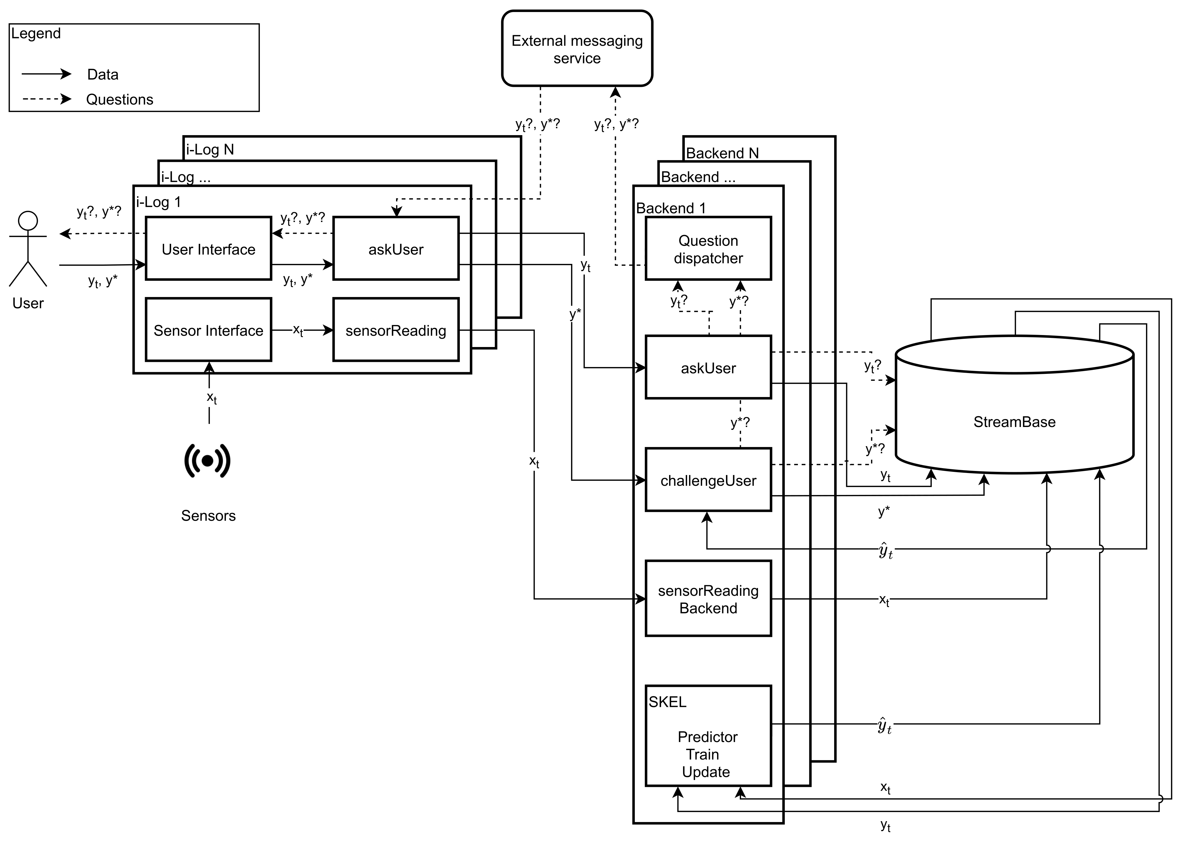
The SkeL platform is depicted in Figure 3. To better understand it, the reader should assume that all processes between components run asynchronously. This platform combines two parts: the i-Log front-end interacting with the world in terms of user and device (left) and a back-end implementing, among others, the SkeL logic (right). There is an instance of i-Log, and corresponding back-end, per user, while there is a single storage for all of the users. Below, we analyze these three components.

3.1. Front-End: i-Log

One of the core functionalities provided by the platform is the ability to acquire knowledge about the world via both sensors and users, and to make these data available for later processing and data analysis. Since the users of the platform are ordinary citizens in the mobile crowd sensing scenarios and may have unreliable behaviors, obtaining information or data with high quality becomes more challenging. As seen in Figure 3, i-Log has two main input elements: the user on one side, which provides annotations in the form of answers y t , y * to questions y t ? , y * ? . The former is a type of question sent at fixed time instants, whose answers are mainly used as standard annotations, whereas the latter is sent on demand, when the system decides to challenge the user. On the other side, there is the world, which is captured through sensors embedded in the smartphone and wearables, generating sensor readings x t . i-Log is composed of four high level components: (1) askUser, (2) sensorReading, (3) the user interface, and (4) the sensor interface. Let us analyze these components in turn.

3.1.1. askUser

The main functionalities of askUser are related to the collection of feedback from the user in the form of answers to questions. Its responsibilities are end-to-end, meaning that it has to deliver the questions y t ? , y * ? to the user (dashed lines in Figure 3), but also to deliver the answers y t , y * to the back-end system (continuous lines in Figure 3). The questions are received from the back-end through an external messaging system, such as Google’s messaging service Firebase (https://firebase.google.com accessed on 24 January 2022), or Baidu Messaging (https://push.baidu.com/ accessed on 24 January 2022), among others. The advantages of using such external services can be summarized in four elements: (1) battery optimization, (2) time to deliver, (3) size of the message, and (4) caching. Concerning battery optimization, Google Firebase has a functionality built in that is responsible for delivering messages in an efficient way in “windows”. It basically consists of a mechanism that groups together messages coming from different applications and delivers all of them together, i.e., to wake up the phone only once when in sleep mode. This leads to important savings in terms of battery life on the device side, since the phone does not need to listen to incoming messages continuously. At the same time, messages are usually delivered in a short time frame, in most cases within few seconds, which is perfect, even for real-time use cases.
Another important aspect to keep under control on mobile devices is the network cost, especially in some countries. If it is true that nowadays it is not uncommon to see data plans for tens of GB, this is not true in all countries around the world. For this reason, the transmission of data should always be optimized and compressed. Firebase helps in this regard since every message has a size limit of 4 KB, which forces the developer to transmit only essential information. Moreover, sending all messages together and compressed reduces the amount of bytes that need to be transferred.
Finally, the last advantage of using an external delivering message system is that, in most situations, i.e., with Firebase and Baidu, a caching system is provided. In fact, smartphones are characterized by intermittent network connections that can leave the device disconnected from the internet multiple times a day for an arbitrary amount of time. Consider, for example, when the user enters a building with no signal, or when the devices switches between cellular networks. In such situations, it is important to have a caching system in place when delivering messages, since, if the message is delivered at the wrong moment in time, when the phone is disconnected, it could get lost. Services such as Firebase provide a robust caching mechanism that can be customized on a per-message basis. We can specify the amount of minutes according to which the message should be delivered, as soon as the device is connected. If this time interval expires and the message has not been delivered, the message itself is discarded. This mechanism is perfect in the situations mentioned above, when the phone disconnects for short periods of time, but it also applies when the user turns off the phone for a period of hours, i.e., during the night.
It is important to underline that this component works in an asynchronous fashion: the questions are received as soon as they are generated by the back-end, but the answers are collected asynchronously, since they involve an action from the user. Finally, this component collects two types of answers: y t , which are time diaries asked at fixed time intervals by the askUser back-end component, and y * , which, instead, are answers to a challenge request by SkeL.

3.1.2. sensorReading

The main functionality of sensorReading is to collect sensor readings x t from the edge device and synchronize them with the back-end system. Similarly to the askUser component, it also works asynchronously: the front-end collects sensor readings from the device continuously, without any input from the back-end, and synchronizes them only at specific moments in time in order to make them available to the back-end and SkeL. This is carried out for different reasons, the most important ones being the battery life of the edge device and the network costs for the user. In fact, depending on the MCS task, x t can be big in size, considering that it can collect up to 30 different sensor streams simultaneously, with frequencies up to 100 Hz . A list of the supported sensor streams is available in Table 1 .

3.1.3. User Interface

The user interface is the component that the user interacts with directly on his/her smartphone when it comes to collecting the user answers to askUser and challengeUser in SkeL. Its main responsibilities are to display a user interface tailored for the specific device that contains the corresponding questions y t ? , y * ? . In the current implementation, there are different question formats that are usable by the system. They all have the question field in common, which is text based. Some of them have additional graphical elements that can support the question, such as images, among others. Finally, the answer field is diverse for each type. The most relevant question formats are: text question with a multiple choice answer (with (1) single and (2) multiple selection allowed), (3) text question with a free text input allowed, (4) text question supported by a map view and a pointer displayed on it with a multiple choice answer, (5) text question supported by a map view and a path displayed on it with a multiple choice answer, and (6) a text question with the possibility for the user to take a picture. An example of the usage of the latter format is presented in [5].
An important feature of the user interface is that it keeps track of the time that the user spends answering each question, i.e., the time duration between when a question is received and when it is answered, and the time taken by the user to answer it, namely the elapsed time between when the user opens a question and when they press the finish button. These two parameters are important because they allow us to filter out invalid answers during the analysis. In [15], the researchers use these two parameters to measure the biases and carelessness in the users’ respondents.
Finally, this component is also in charge of implementing the logic of dependency between questions and answers. This feature is crucial in that it allows us to customize the next question based on the previous answer given by the user. For example, if the user replies to the question “What are you doing?” with “I’m travelling”, then the next question will be “Where are you going?” rather than “Where are you?”. These types of dependencies must be set up in the back-end while generating the sequence of questions.

3.1.4. Sensor Interface

This is the component that interacts directly with the hardware of the edge device, e.g., the accelerometer and the gyroscope. Its main goal is to abstract the hardware from the higher level processes and to generate the streams of sensors data x t . A second main functionality of this component is also to generate streams of what we call “software sensors”. Software sensors are software modules that generate data generated by monitoring the various software modules running on the device. One example of a software sensor is the one that monitors the status (ON/OFF) of the screen, and another one detects the name of the application that is running in foreground, every 5 s, among others.
The sensor interface component is of primary importance to enable a systematic sensor data collection on different edge devices. This applies to both hardware and software sensors. In fact, in each MCS task, we will have multiple smartphone models with different operating system’s versions, since the user uses his/her own personal smartphone. These aspects affect the sensor data collection in two ways: (1) different smartphones have different sensors and (2) even if the sensor set is the same, those sensors will generate data differently on each device. The sensor interface component addresses both. First of all, for each device, it enables only the sensor streams that are present on the smartphone automatically, disabling the other ones. Secondly, it collects data in such a way so that the generated streams are consistent, with a similar collection frequency, amplitude, precision, and so on.

3.2. Back-End

The back-end, as shown in Figure 3, works paired with the front-end part to provide an end-to-end user experience. This is why each user has an instance of the back-end, as well as the front-end. In fact, each user has different parameters that customize the dynamics in the back-end to deliver a tailored user experience. Three out of five components map directly between the front-end and back-end—(1) askUser (and (2) challengeUser), and (3) sensorReading—whereas the other two—(4) Question Dispatcher and (5) SKEL—are only available in the back-end.

3.2.1. askUser

askUser performs two tasks: (1) it accepts answers y t from the device, processing and storing them in the StreamBase database (see the next subsection), while, at the same time (2) triggering questions y t ? at fixed time intervals, tailored on the user. The time interval can vary because different users behave differently: some of them are more reliable in replying and have less variance in their activities throughout the day, whereas others may have a lot of variance or may be unreliable. For the former ones, the system requires less annotations/ answers and the time interval can be kept in the order of 30–60 min, whereas, for the latter, more annotations are required. The content of each question is configurable in the system and is usually experiment-based. Since every MCS task has a different goal, the questions may differ every time. An example of such questions is presented in Table 5 for the evaluation experiment carried on for this paper.

3.2.2. challengeUser

challengeUser, similarly to askUser, accepts answers y * from mobile devices and generates questions y * ? to be sent to the the user. Differently from askUser, the questions are not generated at fixed time intervals but rather on demand, whenever a conflict in the SKEL component arises. When this happens, this component takes the prediction y ^ t from StreamBase, which is generated by SKEL. Then, asynchronously, this component detects a new question and triggers question y * ? to the user.

3.2.3. sensorReading

sensorReading is a component responsible for accepting sensor data x t from the mobile device. The operations it performs are (1) pre-processing the data, (2) normalizing them, and, finally, (3) pushing such data in StreamBase. Due to the size of the data, this component is the one in the back-end that needs the biggest resources.

3.2.4. Question Dispatcher

The question dispatcher is the component that is responsible for efficiently delivering questions y t ? , y * ? to the mobile devices. To carry this out, it relies on external services depending on the need: the system can be easily configured in this regard. Using external services removes an important overhead on our side and allows us to send content to mobile devices efficiently, as previously explained in the front-end part.

3.2.5. SkeL

SkeL is the architectural component that embeds an implementation of the SkeL algorithm. It takes sensor data x t and the user’s answers y t as an input to train the predictor. When new sensor data are generated by the edge devices and synchronized with the server, it generates a prediction label y ^ t . SKEL can detect a conflict by comparing the user’s answer and predictor’s label. When this happens, and the predictor’s confidence is high enough, it triggers challengeUser to generate an additional question to be sent to the user. The user’s answer y * is asynchronously collected and considered as ground truth. It is used to retrain the predictor and to update the confidence value of the user and predictor accordingly.

3.3. StreamBase

StreamBase is the storage solution that is in charge of storing all of the information collected from smart phones. As can be seen in Figure 3, it is part of the back-end system, but it is logically separated from it. In fact, while the back-end has an instance per user, we can consider the database as a unique entity where all of the data are stored, logically separated for privacy reasons. The technology at the core of it is a NoSQL database called Apache Cassandra (https://cassandra.apache.org/ accessed on 24 January 2022). The reason why we decided to adopt it is that the amount of information and the growth rate can be significant, even with a limited amount of users for our use-cases. For this reason, standard solutions based on SQL could not satisfy the requirements in terms of latency and scalability. In the current configuration, Cassandra is distributed on multiple nodes in the cloud, thus allowing us to handle huge bursts in the number of requests. Three main types of information are stored in Cassandra, all as streams of data with an attached timestamp: (1) sensor values x t , (2) questions y x ? , and (3) answers y t . Let us analyze these types of data in turn.
Sensor values are the biggest in size, mainly due to their frequency. Depending on the configuration of the MCS task, we can have the inertial sensors generating values that add up to 100 Hz. All such data are stored in the database as time series. There are two columns common to every other sensor: the timestamp and day. The former is used to allow temporal queries, whereas the latter is used as a partition key in Cassandra to balance the data in the different distributed nodes composing the cluster. The remaining columns are different for every sensor. For example, in Table 2, we present the structure of the inertial sensors used to identify the movement of the smartphone, the accelerometer.
The second type of data stored is the questions that are asked to the user. It is important to keep track of them with the proper provenance information in order to reconstruct the flow from the system to the user. In this regard, the question IDs are essential to the SKEL algorithm. An additional field present is the status of the question, which can be either DELIVERED, SENT, or DISCARDED. Apart from these, we have the “question” field, which contains the text that was shown to the user, and the “timestamp”, which is the time when the question was generated in the back-end. An example of questions stored in the database can be seen in Table 3.
The last type of data in the StreamBase storage system is the answers to the questions generated by the askUser and challengeUser components. An example of such data can be seen in Table 4. The “day” field is common to the other types of data. We then have the “answer” and “payload”, which, respectively, contain the text response and any additional response element that the user provided, i.e., a picture, information on a map, etc. We then have the “question id”, which links the answer to the corresponding question, as presented in Table 3. Finally, we have multiple columns that define time variables: “question timestamp” is the same as in the question table, which refers to the time at which the question was generated and sent to the device; “notification timestamp” refers to the time when the front-end received the question (usually within a few seconds if the phone is turned on and connected), and, finally, the “answer timestamp”, which is the time when the user answers the question. Two additional fields are present, delta and duration, which map to the answering behavior of the users, as explained in the front-end part previously in the paper.
Obviously, most of the data in the storage system that refer to the user are sensitive information. However, in the contest of GDPR and personal data, none of them are considered to be a personal identifier, except for the user email, which we store for technical purposes. In fact, the email is used to authenticate all of the requests coming from the front-end applications. In the i-Log application, the user is required to login with Google Identity (https://developers.google.com/identity accessed on 24 January 2022) anywhere in the world except for China (where Baidu Login (https://login.bce.baidu.com/ accessed on 24 January 2022) is used instead.). At every request, a token is sent and the server uses it to extract the user email, which is then used to understand under which user to store the data in the main database. To comply with the regulations, we split the email identifier from the main storage system through an intermediate table in MySQL. This table has only two columns: the personal identifier (email) and a uuid. Whenever a user registers in the system, a random uuid is generated and a row is added to this table. All of the data in the StreamBase system based on Cassandra are then stored according to that uuid. Whenever the need to link the data to the email address expires, the corresponding line in the intermediate table is removed and the data in Cassandra immediately become anonymous and cannot be linked back to the user who generated it.

4. The Experiment on the SkeL Platform

The platform has been used and tested in a large number of experiments. Thus, for instance, in the work described in [16], crowdsensing and crowdsourcing have been combined in order to identify and localise WiFi networks. In the work described in [5], the platform has been used to implement two hybrid human–machine workflows for solving two mobility problems: modal split estimation and mapping mobility infrastructure. Last but not least, the platform has been used in a large scale personal data collection experiment, run by Eurostat, aimed at feeding a Europe-wide big data hackathon [17]. In this paper, we concentrate on one of a series of MCS experiments run at the University of Trento whose goal was to study the effects of students’ behavior and habits on their academic performance. The main reason for this choice relates to the fact that, in the case of personal data, it is easier to collect feedback, as this activity involves only the user of each single device.
The highlights of the experiment are as follows. Out of an initial population of 312 students, 72 were selected who satisfied three specific criteria, namely, their willingness to share personal information, the fact that they were actively attending classes, and that their phone could support the i-Log application. The cohort was designed to reflect the general population of students in terms of gender and field of study. The experiment lasted two weeks. During the first week, students were asked to answer a specific questionnaire every half an hour, and the answers were the labels used by SkeL. Meanwhile, i-Log would keep collecting the sensor data from their smartphone. During the second week, students only needed to keep the application running in the background for the sensor data collection. The sensors used in the experiment are those listed in Table 1. The resulting dataset has a total size of 110 GB, containing 20 billion sensor values plus the user answers to the time diaries’ questions, which are considered as an annotation to the sensor data. The total number of answers generated during the experiment is 17,207 out of 27,111 sent.
Table 5 shows the questionnaire that users had to answer during the first week. The design of the questionnaire follows the context model from [18]. It is composed of three questions, namely “What are you doing?”, “Where are you?”, and “Who is with you?”. Notice that, if the user’s answer of the activity was “En route”, the user was further asked about the transportation mode. The user could choose, as his/her answer, one of a pre-selected list of labels. The user’s answers were meant to help in the understanding of the user situational context and its aspects relating to his/her activity, location, and social relations.

5. Evaluation

In the evaluation, we only focus on the user’s annotation to the location and transportation means, namely, the labels generated as answers to the questions in the second column in Table 5. The evaluation consists of two parts: proving (1) that annotation mistakes from non-expert users are a quantitatively major problem (Section 5.1), and proving that (2) SkeL is able to detect and mitigate the effect of such mistakes (Section 5.2). This evaluation is based on the following assumptions:
  • The SkeL algorithm is evaluated asynchronously, at the end of each day;
  • The SkeL algorithm uses, in any moment, all of the data previously collected, without an explicit “forget” mechanism for old data. This is because removing old data helps in adapting to users’ changes in behavior and patterns. However, since the data were generated from an experiment lasting 2 weeks, this was not needed;
  • The knowledge of the world SK available to the SkeL algorithm was a simplified sub-set of the available one, with elements related to only the use-case (see Figure 2). Moreover, we considered it to be static for the whole duration of the experiment, and not evolving over time.

5.1. Pervasiveness of Annotation Mistakes

The analysis of the collected answers is performed by comparing them with a ground truth. To have a ground-truth independent of both the predictor and the user annotation, we focus on predicting the locations participants visited during the two weeks of the experiment and those transportation activities related to movements across such locations. We use a hierarchy of labels from SK that accounts for both the user location and the user transportation means, as reported in Figure 2. We have computed ground-truth labels for university by using maps of university buildings. The ground-truth of the user’s home has been computed by clustering locations via DBSCAN [19]. We choose the coordinates of locations that the user labels as “home” as the inputs to the DBSCAN algorithm, and it outputs a set of clusters according to the density of these coordinates on the map. The distance we choose for clustering locations is 108.27 m, as it is the average accuracy of the considered locations. Then, the cluster on which the user spends most of the time during the night will be chosen as the ground-truth of the user’s home. Using Google data (for users that agreed to provide them, i.e., 32 out of 72), we have also been able to detect if the user was on the move, and whether he/she was moving on foot, by bike, or in vehicle. Finally, the Other location label has been assigned to the cases in which none of the other three main locations were detected. Note that SKEL has no access to the information used to compute the ground truth.
The analysis in Table 6 provides evidence that a surprisingly high proportion of labels were inconsistent. Table 6 shows some statistics on the percentage of users with different amounts of labeling noise. The results in Table 6 validate, beyond our initial expectations, our hypothesis that non-expert users consistently and systematically makes mistakes while providing annotations, with only 21.6 % of the users having less than 10 % of labeling mistakes.

5.2. The Algorithm

The next component to be evaluated is the SkeL algorithm. As discussed in Section 2, the Pred procedure of SkeL consists of a hierarchy of multiclass classifiers, one for each internal node in the hierarchy. Each classifier implemented a random forest [20], which is known to be robust to labeling noise [21], to evaluate the ability of SkeL to improve over an already noise-robust baseline. The confidence parameter θ of SkeL has been set to 0.2, which has resulted in a reasonable trade-off between accurate training and cognitive effort for the user. For simplicity, we have used an infinite queue ( d = ) for the confidence update due to the relatively short duration of the experiment. This being an experiment built on previously collected data, we could not query users in real-time in case of conflicts. To simulate a collaborative, non-adversarial user, we assumed that the user returns the ground truth label when his/her initial label is contested.
The evaluation of SkeL is performed by comparing it with three alternative algorithms:
  • NonSkeL, which never contradicts the user (obtained by replacing solveConflict with a train and update step, as occurs in the training phase);
  • Ignore, which simply ignores any example for which a conflict arises (obtained by removing everything from the else onwards in Algorithm 3);
  • Bother, which always contradicts the user (obtained by calling challengeUser after all askUser calls, and removing solveConflict.
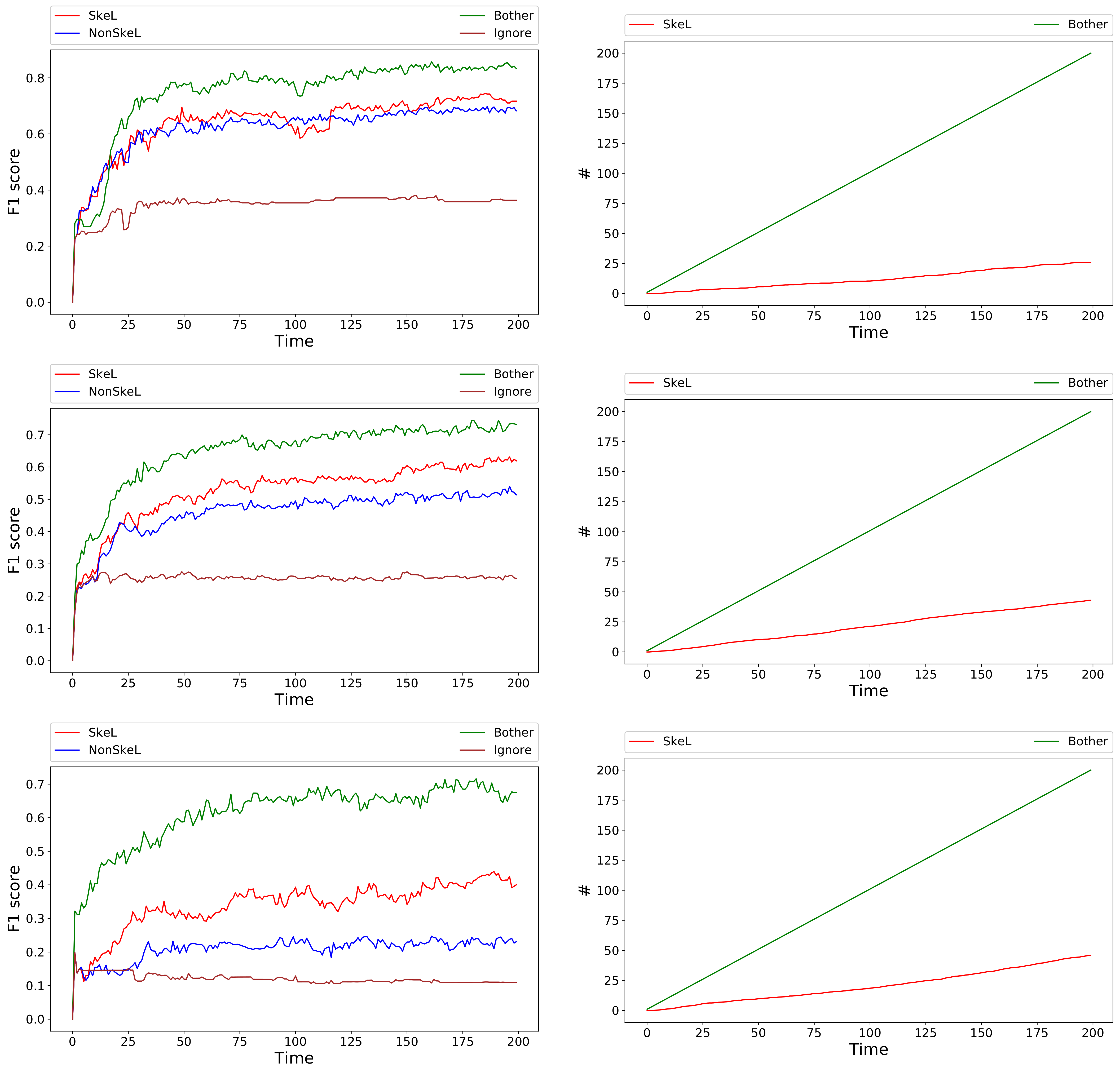
As presented in the previous section, a surprisingly high proportion of labels present inconsistencies. To estimate the effect of this large and very diverse proportion of labeling errors on the performance of the system, we divided the set of users in the three groups reported in the table. Figure 4 reports the results of SkeL and of the three alternatives for an increasing number of iterations. Each row represents the results for a different group of users: at most 10% labeling errors (top), 10% to 25% (middle), more than 25% (bottom). The left column reports f 1 scores averaged over all users in the corresponding group with a number of training samples greater than 200. The score for each user is computed on a fixed test set, namely the latest 15 % of all of the data available for that user that were not used for training. This score provides an estimate of the performance of the algorithms when making predictions on future data. Note that we consider a label as correctly predicted if it is compatible with the ground-truth label, because this is the only type of reliable supervision we have access to. Results clearly indicate that our skeptical algorithm (red curve) consistently outperforms a non-skeptical alternative (blue curve). As expected, the advantage is moderate for users with a relatively small fraction of labeling errors (top figure), and grows with the unreliability of the users, reaching a gap of 0.20 for users with more than 25% labeling errors (bottom figure). Ignoring conflicting cases (brown curve) is clearly not an option, as it achieves the worst performance in all cases. On the other hand, when always having access to correct supervision, Bother (green curve) clearly achieves the highest performance. However, SkeL is capable of getting reasonably close to this upper bound when enough iterations are provided, at a fraction of the cost in terms of user effort. The right column reports the number of times the user is contradicted for SkeL (red curve) and for Bother (green curve), for which, they are simply the number of iterations. SkeL clearly contradicts more when facing increasingly unreliable users. However, the cost remains substantially lower than that of Bother, going from 13 % (top figure) to 23 % (bottom figure).
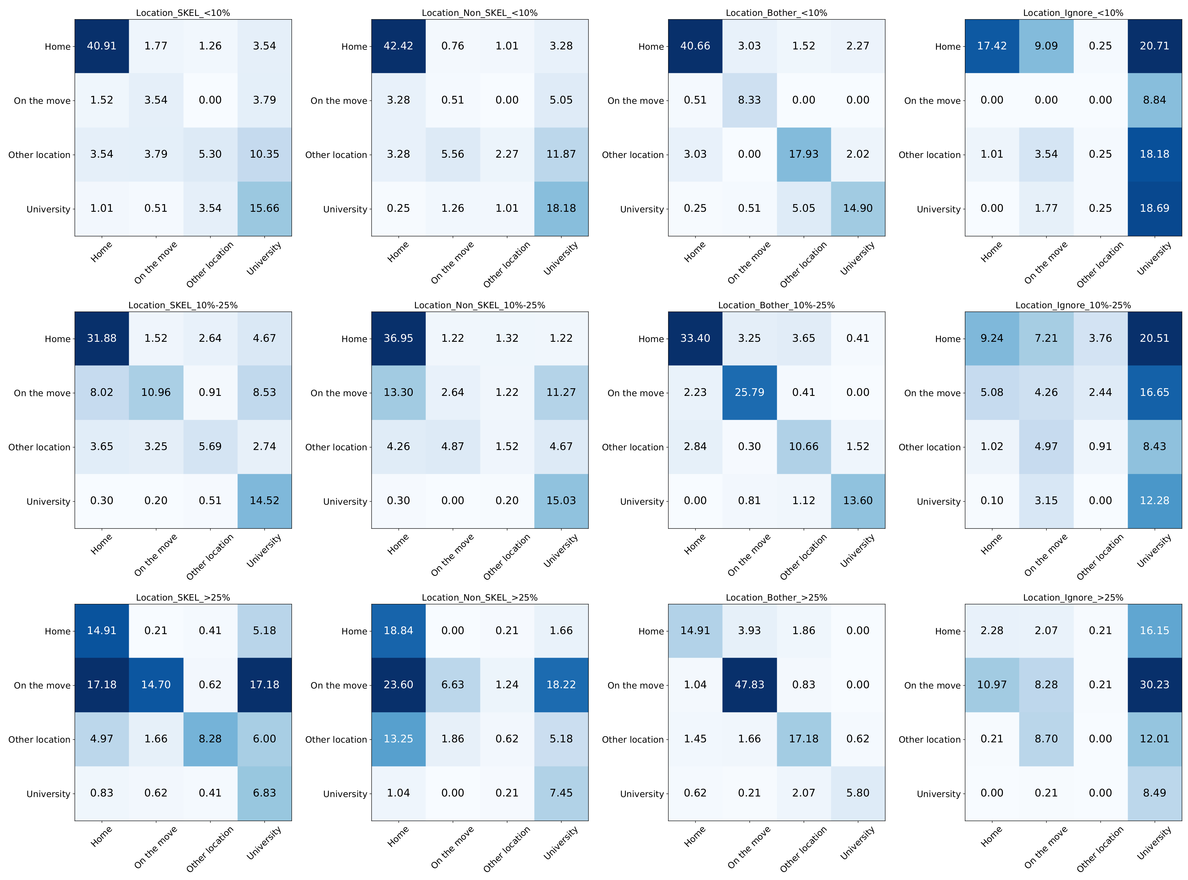
Figure 5 reports the confusion matrices of the location classifier (the root of the hierarchy in Figure 2) for the last time instant of the different algorithms shown in Figure 4. Results are normalized over the sum of all of the elements in the matrix. In each matrix, rows are ground truth labels and columns are predicted labels. Matrix entries are colored, with darker shades corresponding to larger entries. Each row represents the results for a different group of users who have, at most 10%, from 10% to 25%, and more than 25% labeling errors, respectively. The matrices in the first column report results of the SkeL algorithm, the second column report results of the NonSkeL one, the third column report results of the Bother one, and the last column report results of the Ignore one.
Clearly, Bother has the best performance, as can be seen by the dark coloring of the main diagonal (corresponding to correct predictions), and shows the upper limit one can reach by always having access to the ground truth during training. While not as accurate, SkeL has a similar qualitative behavior, with on-diagonal entries typically larger than off-diagonal ones. The bad performance of Ignore and NonSkeL are due to the fact that they tend to overpredict certain classes (as shown by the dark columns): University and On the Move for Ignore, University and Home for NonSkeL.
The first row represents the results of the users with fewer labeling errors. Given that these users tend to provide high-quality labels, SkeL is only slightly better than NonSkeL. This is consistent with the F 1 score in the first row of Figure 4, where the red curve and blue curve are close to each other. However, SkeL manages to substantially improve the recognition ability for On the move and Other location, the classes for which the user feedback is least frequent, at the cost of a (smaller) decrease in accuracy for the most popular ones, University and Home. This behavior is even more evident when considering users with a higher fraction of errors (middle row, from 10% to 25% labeling errors), where the fraction of times On the move and Other location get predicted and the prediction is correct increases from 2.64% to 10.96% and from 1.52% to 5.69%, respectively. The third row reports results for the least reliable users, with more than 25% labeling errors. While the distance to the “ideal” (for the machine) setting represented by Bother increases, the advantage of SkeL over NonSkeL (and Ignore) also widens. The tendency of the user to always reply with Home and University does affect SkeL, which starts to show a similar behavior (dark columns in the matrix). On the other hand, despite the substantial unreliability of the user feedback, it still manages to recover a large fraction of the On the Move (from 6.63% to 14.70%) and the Other location (from 0.62% to 8.28%) classes, both virtually lost by NonSkeL.

6. Discussion

Whereas traditional approaches assume perfectly labeled training sets, most recent supervised learning techniques can tolerate a small fraction of mislabelled training instances (see, for instance, [22]). A common solution consists of designing learning models that are robust to (some) label noise [23]. In particular, by averaging predictions of multiple learners, ensemble methods usually perform well in terms of noise robustness [24,25]. In this line of thought, the robustness of random forests, the ensemble method used in this paper, has recently been shown both theoretically and empirically [21]. Nonetheless, label noise badly affects the performance of learning algorithms [26]. Our approach diverges from existing solutions since it involves an interactive error correction phase. This process allows for the tolerating of a much larger amount of noise, achieving substantial improvements over the previous work.
The field of statistical relational learning [27] deals with the integration of symbolic and sub-symbolic approaches to learning. Frameworks such as Markov logics [28], semantic-based regularization [29], or learning modulo theories [30] combine logical rules or other types of constraints with learnable weights to encourage predictions consistent with the available knowledge. Our main difference is that we use knowledge in an interactive way to identify potential errors in the user feedback, and activate a conflict resolution phase to solve such controversies.
As already pointed out in the introduction, in MCS systems, a major problem is the quality of the data. Inconsistent data could have a negative effect on the accuracy and performance of machine learning systems, even leading to a decrease in the intelligence of the system [31]. In [32], the authors deal with this problem by computing the reputation score of the device as a reflection of the trustworthiness of the contributed data. Dually, in [33], the reputation system focuses on the reputation of the human participants. Differently from this work, we propose a hybrid approach, where we evaluate both the users and the machine and deal with personal data, and our metrics leading to reputation are the result of a machine learning activity.
Concerning the experiment used to construct the evaluation data set, the closest and most relevant research work is the Student Life study [34], where the authors have developed a continuous sensing app called StudentLife running on smartphones. This experiment was carried at the Dartmouth College for 10 weeks and it involved 48 students. The researchers assessed the impact of workload on stress, sleep, activity, mood, sociability, mental well-being, and academic performance. A similar work is the SmartGPA study [35], which performed a time series analysis on the dataset published in [34]. The goal of this work was to find which behavior had the highest impact on the students’ GPA. Moreover, they proposed a linear regression model that was used to predict the student’s GPA based on their behavior. However, in none of these research studies did the authors evaluate the quality of the annotations from the students, and, therefore, did not deal with the mislabeling problem.

7. Conclusions

In this paper, we have introduced a general MCS platform that, together with the i-Log application, can be used to collect sensor data and user’s annotations. On top of them, the platform runs SkeL, a machine learning algorithm that deals with the unreliability of non-expert users when providing labels. The fundamental idea is to use the available knowledge when deciding what is more reliable between the output of the machine learning algorithms and the user input, and to engage in a conflict resolution phase when a controversy arises. The experimental results show the pervasiveness of mislabeling when dealing with feedback from non-expert users, as well as the effectiveness of SkeL in addressing the problem, as compared to existing approaches that deal with noisy labels.

Author Contributions

Data curation, M.Z.; Methodology, W.Z., M.Z., A.P. and F.G.; Software, M.Z.; Supervision, A.P. and F.G.; Validation, W.Z.; Writing—original draft, W.Z. and M.Z.; Writing—review & editing, A.P. and F.G. All authors have read and agreed to the published version of the manuscript.

Funding

This research was funded by the European Union’s Horizon 2020 FET Proactive project “ WeNet—The Internet of us”, grant agreement No. 823783, and the “DELPhi—DiscovEring Life Patterns” project funded by the MIUR progetti di Ricerca di Rilevante Interesse Nazionale (PRIN) 2017—DD n. 1062 del 31.05.2019.

Institutional Review Board Statement

Not applicable.

Informed Consent Statement

Not applicable.

Data Availability Statement

Not applicable.

Conflicts of Interest

The authors declare no conflict of interest.

References

  1. Guo, B.; Yu, Z.; Zhou, X.; Zhang, D. From participatory sensing to mobile crowd sensing. In Proceedings of the 2014 IEEE International Conference on Pervasive Computing and Communication Workshops (PERCOM WORKSHOPS), Budapest, Hungary, 24–28 March 2014; pp. 593–598. [Google Scholar]
  2. Feng, C.; Tian, Y.; Gong, X.; Que, X.; Wang, W. MCS-RF: Mobile crowdsensing–based air quality estimation with random forest. Int. J. Distrib. Sens. Netw. 2018, 14, 1550147718804702. [Google Scholar]
  3. Kraft, R.; Schlee, W.; Stach, M.; Reichert, M.; Langguth, B.; Baumeister, H.; Probst, T.; Hannemann, R.; Pryss, R. Combining mobile crowdsensing and ecological momentary assessments in the healthcare domain. Front. Neurosci. 2020, 14, 164. [Google Scholar] [PubMed]
  4. Zhao, X.; Wang, N.; Han, R.; Xie, B.; Yu, Y.; Li, M.; Ou, J. Urban infrastructure safety system based on mobile crowdsensing. Int. J. Disaster Risk Reduct. 2018, 27, 427–438. [Google Scholar]
  5. Maddalena, E.; Ibáñez, L.D.; Simperl, E.; Gomer, R.; Zeni, M.; Song, D.; Giunchiglia, F. Hybrid Human Machine workflows for mobility management. In Proceedings of the 2019 World Wide Web Conference, San Francisco, CA, USA, 13–17 May 2019; pp. 102–109. [Google Scholar]
  6. West, B.T.; Sinibaldi, J. The quality of paradata: A literature review. Improv. Surv. Parad. 2013, 339–359. [Google Scholar]
  7. Tourangeau, R.; Rips, L.J.; Rasinski, K. The Psychology of Survey Response; Cambridge University Press: Cambridge, UK, 2000. [Google Scholar]
  8. Baader, F.; Calvanese, D.; McGuinness, D.; Patel-Schneider, P.; Nardi, D. The Description Logic Handbook: Theory, Implementation and Applications; Cambridge University Press: Cambridge, UK, 2003. [Google Scholar]
  9. Zeni, M.; Zhang, W.; Bignotti, E.; Passerini, A.; Giunchiglia, F. Fixing Mislabeling by Human Annotators Leveraging Conflict Resolution and Prior Knowledge. Proc. ACM Interact. Mob. Wearable Ubiquitous Technol. 2019, 3, 32. [Google Scholar]
  10. Zhang, W.; Passerini, A.; Giunchiglia, F. Dealing with Mislabeling via Interactive Machine Learning. Ki-KÜNstliche Intell. 2020, 34, 271–278. [Google Scholar]
  11. Zeni, M.; Zaihrayeu, I.; Giunchiglia, F. Multi-device activity logging. In Proceedings of the 2014 ACM International Joint Conference on Pervasive and Ubiquitous Computing: Adjunct Publication, Seattle, WA, USA, 13–17 September 2014; pp. 299–302. [Google Scholar]
  12. Giunchiglia, F.; Batsuren, K.; Bella, G. Understanding and Exploiting Language Diversity. In Proceedings of the Twenty-Sixth International Joint Conference on Artificial Intelligence (IJCAI-17), Melbourne, Australia, 19–25 August 2017; pp. 4009–4017. [Google Scholar]
  13. Shalev-Shwartz, S. Online Learning and Online Convex Optimization. Found. Trends Mach. Learn. 2012, 4, 107–194. [Google Scholar] [CrossRef]
  14. Settles, B. Active Learning Literature Survey; Computer Sciences Technical Report 1648; University of Wisconsin–Madison: Madison, WI, USA, 2009. [Google Scholar]
  15. Giunchiglia, F.; Zeni, M.; Gobbi, E.; Bignotti, E.; Bison, I. Mobile Social Media and Academic Performance. In International Conference on Social Informatics; Springer: Berlin/Heidelberg, Germany, 2017; pp. 3–13. [Google Scholar]
  16. Maddalena, E.; Ibáñez, L.D.; Simperl, E.; Zeni, M.; Bignotti, E.; Giunchiglia, F.; Stadler, C.; Westphal, P.; Garcia, L.P.; Lehmann, J. QROWD: Because Big Data Integration is Humanly Possible. In Proceedings of the Project Showcase Track of KDD2018, London, UK, 19–23 August 2018. [Google Scholar]
  17. Zeni, M.; Bison, I.; Gauckler, B.; Reis, F.; Giunchiglia, F. Improving time use measurement with personal big data collection— The experience of the European Big Data Hackathon 2019. arXiv 2019, arXiv:2004.11940. [Google Scholar]
  18. Giunchiglia, F.; Bignotti, E.; Zeni, M. Personal context modelling and annotation. In Proceedings of the 2017 IEEE International Conference on Pervasive Computing and Communications Workshops (PerCom Workshops), Kona, HI, USA, 13–17 March 2017; pp. 117–122. [Google Scholar]
  19. Ester, M.; Kriegel, H.P.; Sander, J.; Xu, X. A density-based algorithm for discovering clusters in large spatial databases with noise. KDD 1996, 96, 226–231. [Google Scholar]
  20. Breiman, L. Random Forests. Mach. Learn. 2001, 45, 5–32. [Google Scholar] [CrossRef] [Green Version]
  21. Ghosh, A.; Manwani, N.; Sastry, P.S. On the Robustness of Decision Tree Learning Under Label Noise. In Advances in Knowledge Discovery and Data Mining; Kim, J., Shim, K., Cao, L., Lee, J.G., Lin, X., Moon, Y.S., Eds.; Springer International Publishing: Cham, Switzerland, 2017; pp. 685–697. [Google Scholar]
  22. Frénay, B.; Kabán, A. A comprehensive introduction to label noise. In Proceedings of the ESANN 2014: European Symposium on Artificial Neural Networks, Computational Intelligence and Machine Learning, Bruges, Belgium, 23–25 April 2014. [Google Scholar]
  23. Folleco, A.; Khoshgoftaar, T.M.; Hulse, J.V.; Bullard, L. Identifying learners robust to low quality data. In Proceedings of the 2008 IEEE International Conference on Information Reuse and Integration, Las Vegas, NV, USA, 13–15 July 2008; pp. 190–195. [Google Scholar] [CrossRef]
  24. Dietterich, T.G. An Experimental Comparison of Three Methods for Constructing Ensembles of Decision Trees: Bagging, Boosting, and Randomization. Mach. Learn. 2000, 40, 139–157. [Google Scholar] [CrossRef]
  25. Rätsch, G.; Schölkopf, B.; Smola, A.J.; Mika, S.; Onoda, T.; Müller, K.R. Robust Ensemble Learning for Data Mining. In Knowledge Discovery and Data Mining. Current Issues and New Applications; Terano, T., Liu, H., Chen, A.L.P., Eds.; Springer: Berlin/Heidelberg, Germany, 2000; pp. 341–344. [Google Scholar]
  26. Nettleton, D.F.; Orriols-Puig, A.; Fornells, A. A study of the effect of different types of noise on the precision of supervised learning techniques. Artif. Intell. Rev. 2010, 33, 275–306. [Google Scholar] [CrossRef]
  27. Bakir, G.H.; Hofmann, T.; Schölkopf, B.; Smola, A.J.; Taskar, B.; Vishwanathan, S.V.N. Predicting Structured Data (Neural Information Processing); The MIT Press: Cambridge, MA, USA, 2007. [Google Scholar]
  28. Richardson, M.; Domingos, P. Markov logic networks. Mach. Learn. 2006, 62, 107–136. [Google Scholar] [CrossRef] [Green Version]
  29. Diligenti, M.; Gori, M.; Saccà, C. Semantic-based regularization for learning and inference. Artif. Intell. 2017, 244, 143–165. [Google Scholar] [CrossRef]
  30. Teso, S.; Sebastiani, R.; Passerini, A. Structured learning modulo theories. Artif. Intell. 2017, 244, 166–187. [Google Scholar] [CrossRef] [Green Version]
  31. Iantovics, L.B.; Iakovidis, D.K.; Nechita, E. II-Learn—A Novel Metric for Measuring the Intelligence Increase and Evolution of Artificial Learning Systems. Int. J. Comput. Intell. Syst. 2019, 12, 1323. [Google Scholar]
  32. Huang, K.L.; Kanhere, S.S.; Hu, W. Are you contributing trustworthy data? The case for a reputation system in participatory sensing. In Proceedings of the 13th ACM International Conference on Modeling, Analysis, and Simulation of Wireless and Mobile Systems, Bodrum, Turkey, 17–21 October 2010; pp. 14–22. [Google Scholar]
  33. Yang, H.; Zhang, J.; Roe, P. Using reputation management in participatory sensing for data classification. Procedia Comput. Sci. 2011, 5, 190–197. [Google Scholar]
  34. Wang, R.; Chen, F.; Chen, Z.; Li, T.; Harari, G.; Tignor, S.; Zhou, X.; Ben-Zeev, D.; Campbell, A.T. StudentLife: Assessing mental health, academic performance and behavioral trends of college students using smartphones. In Proceedings of the 2014 ACM International Joint Conference on Pervasive and Ubiquitous Computing, Seattle, WA, USA, 13–17 September 2014; pp. 3–14. [Google Scholar]
  35. Wang, R.; Harari, G.; Hao, P.; Zhou, X.; Campbell, A.T. SmartGPA: How smartphones can assess and predict academic performance of college students. In Proceedings of the 2015 ACM International Joint Conference on Pervasive and Ubiquitous Computing, Osaka, Japan, 7–11 September 2015; pp. 295–306. [Google Scholar]
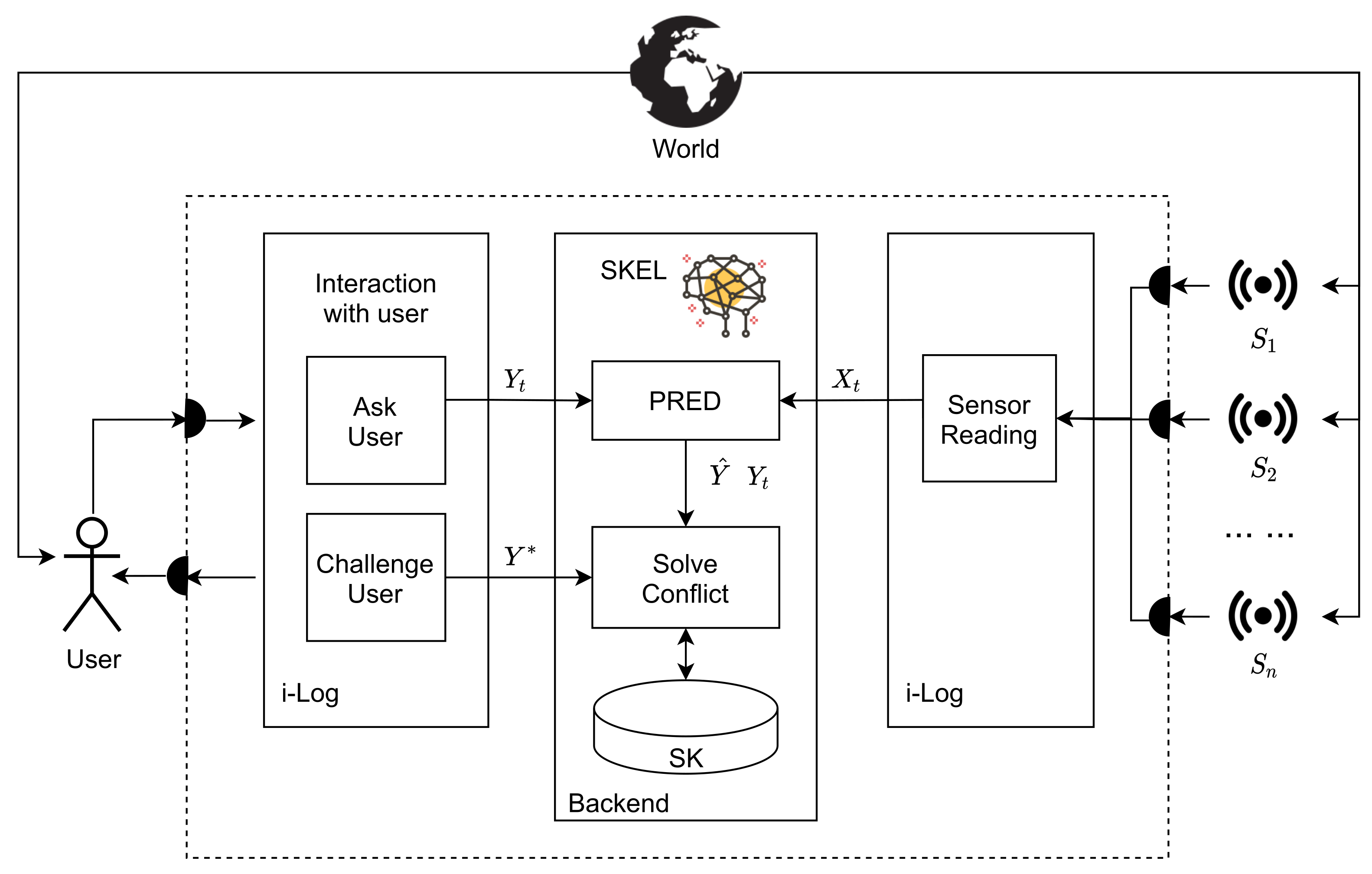
Figure 1. The main components of the system.
Algorithms 15 00109 g001
Figure 2. Ontology of the labels used in the experiment. Bold contours correspond to classifiers in the Pred procedure.
Algorithms 15 00109 g002
Figure 3. The platform architecture.
Algorithms 15 00109 g003
Figure 4. Results averaged over users with at most 10% (top row), from 10% to 25% (middle row), and more than 25% (bottom row) labeling errors. Left column: F 1 scores on left-out data. Right column: number of times user is contradicted.
Algorithms 15 00109 g004
Figure 5. Confusion matrices for the evaluation on ground truth labels at the last iteration of the algorithms. Ground truth labels are on the rows, predicted labels are on the columns. All of the matrices refer to the location classifier and are normalized over all entries.
Algorithms 15 00109 g005
Table 1. Sensors and sampling rate, as used in the experiment.
SensorFrequencySensorFrequencySensorFrequency
Acceleration20 HzScreen StatusOn changeProximityOn change
Linear Acceleration20 HzFlight ModeOn changeIncoming CallsOn change
Gyroscope20 HzAudio ModeOn changeOutgoing CallsOn change
Gravity20 HzBattery ChargeOn changeIncoming SmsOn change
Rotation Vector20 HzBattery LevelOn changeOutgoing SmsOn change
Magnetic Field20 HzDoze ModalityOn changeNotificationsOn change
Orientation20 HzHeadset plugged inOn changeBluetooth Device AvailableOnce every
minute
Temperature20 HzMusic PlaybackOn changeBluetooth Device Available
(Low Energy)
Once every
minute
Atmospheric Pressure20 HzWIFI Networks AvailableOnce every
minute
Running ApplicationOnce every
5 s
Humidity20 HzWIFI Network Connected toOn changeLocationOnce every
minute
Table 2. Accelerometer sensor data stored in StreamBase.
DayTimestampXYZ
20200118202001181005009.180.000.01
20200120202001201256030.896.184.04
20200120202001201205002.742.019.20
20200120202001201318362.940.3215.86
Table 3. Questions stored in StreamBase.
DayQuestionTimestampIdStatus
20200118{“q”: “What are”}20200118100500aDFQivswqAdelivered
20200119{“q”: “What are”}20200119200500ELYs/3HeJYdelivered
20200120{“q”: “Were you”}20200120125603pmQXTjxrLAdelivered
20200120{“q”: “What are”}20200120120500tLN6iIQpdzdelivered
20200120{“q”: “Were you”}20200120131836Yw6q7KXw3csent
Table 4. Answers stored in StreamBase.
DayAnswerPayloadQuestion TimestampNotification
Timestamp
20200118{“a”: “Eating”}{}2020011810050020200118100509
20200119{“a”: “Sport”}{}2020011920050020200119200505
20200120{“a”: “Yes”}{}2020012012560320200120125612
20200120{“a”: “TV”}{}2020012012050020200120120601
20200120{“a”: “No”}{}2020012013183620200120132834
Answer TimestampQuestion IdDeltaDuration
20200118101009aDFQivswqA30065
20200119201505ELYs/3HeJY6005
20200120131612pmQXTjxrLA120098
20200120120701tLN6iIQpdz6023
20200120132849Yw6q7KXw3c15304
Table 5. The questionnaire. (* When the user’s answer to activity is “En route”, the next question to the user will be “How are you traveling?” instead of “Where are you?”)
What Are You Doing?Where Are You?Who Is with You?
LessonClassAlone
StudyStudy hallClassmate(s)
EatingLibraryFriend(s)
Personal careOther university placeRoomate(s)
En route (*)CanteenPartner(s)
Social lifeBar/Pub/etcRelative(s)
Social media and internetHomeColleague(s)
Cultural activitiesOther homeOther
SportWorkplace
ShoppingOutdoors
HobbiesGym
Other free timeShop
WorkOther place
Housework(*) How Are You Traveling?
VolunteeringBy foot
OthersBy bus
By train
By car
By motorbike
By bike
Other
Table 6. Percentage of users with each label noise level.
Label Noise Level≤10%10– 25 % ≥25%
Users 21.6 % 51.4 % 27.0 %
Publisher’s Note: MDPI stays neutral with regard to jurisdictional claims in published maps and institutional affiliations.