Abstract
Background: K-mer frequency counting is an upstream process of many bioinformatics data analysis workflows. KMC3 and CHTKC are the representative partition-based k-mer counting and non-partition-based k-mer counting algorithms, respectively. This paper evaluates the two algorithms and presents their best applicable scenarios and potential improvements using multiple hardware contexts and datasets. Results: KMC3 uses less memory and runs faster than CHTKC on a regular configuration server. CHTKC is efficient on high-performance computing platforms with high available memory, multi-thread, and low IO bandwidth. When tested with various datasets, KMC3 is less sensitive to the number of distinct k-mers and is more efficient for tasks with relatively low sequencing quality and long k-mer. CHTKC performs better than KMC3 in counting assignments with large-scale datasets, high sequencing quality, and short k-mer. Both algorithms are affected by IO bandwidth, and decreasing the influence of the IO bottleneck is critical as our tests show improvement by filtering and compressing consecutive first-occurring k-mers in KMC3. Conclusions: KMC3 is more competitive for running counter on ordinary hardware resources, and CHTKC is more competitive for counting k-mers in super-scale datasets on higher-performance computing platforms. Reducing the influence of the IO bottleneck is essential for optimizing the k-mer counting algorithm, and filtering and compressing low-frequency k-mers is critical in relieving IO impact.
1. Introduction
K-mers are the substrings of length k of a given sequence, and the k-mers in the DNA sequence can be treated like the words of DNA []. K-mer counter is a fundamental tool for analyzing sequencing data [,,] or assembled genomes [,,]. A variety of k-mer counting approaches have emerged in the past decades, including Tallymer [], Jellyfish [], BFCounter [], KMC [,,], DSK [], Turtle [], KAnalyze [], GenomeTester4 [], khmer [], KCMBT [], Gerbil [], CHTKC [], and KCOSS []. K-mer frequency counting is a storage-consuming task, and the storage consumption includes input data, k-mers, and frequency. The memory footprint mainly comes from the storage of k-mers, whereas reading data and saving frequency only accounts for a small proportion. The maximum storage consumption is 4k Bytes when storing k-mers directly. Therefore, many k-mer counting algorithms filter low-frequency k-mers or compress k-mers to reduce memory overhead []. Writing part of uncounted k-mers or frequency to disk is also an alternative way to reduce memory usage [].
K-mer searching is the very core operation of the frequency counting algorithm. Some algorithms distribute k-mers into different partitions to reduce the search range and use efficient data structures to speed up the searching [,,,]. Based on whether the algorithm partitions the k-mers, we classify the k-mer frequency counting algorithms into two categories: partition-based k-mer counting (PBKMC) and non-partition-based k-mer counting (NPBKMC). The parallel PBKMC algorithm for a shared memory environment distributes k-mers into multiple partitions and counts all parts in parallel. When memory is limited, the PBKMC algorithm writes partitions to disk. Since the k-mers of all divisions have no intersection, the algorithm only needs to concatenate the result of each part to obtain the final frequency. The partition-based k-mer frequency counting algorithm is easily affected by the data skew between partitions; therefore, load balance is necessary to improve the algorithm’s robustness. DSK [], MSPKmerCounter [], and KMC [,,] are typical PBKMC algorithms. KMC has been updated many times, and the current version is KMC3 [], which made several significant improvements in partition and counting. A modified minimizer called signature makes KMC3 more robust against data skew than minimizer. In the counting stage, KMC3 uses an efficient parallel radix sort algorithm, Raduls [], to sort and count k-mers in each partition. KMC3 demonstrates the best time and space efficiency and is the state-of-the-art implementation of the PBKMC algorithm. Although the partitioning strategy can reduce memory usage, it may lead to high IO overhead and more time consumption [].
By using a large-capacity and thread-shared memory to store key-value pairs, the NPBKMC algorithm also writes part of uncounted k-mers or frequency to disk to relieve memory requirement. However, the NPBKMC algorithm is sensitive to the number of distinct k-mers. When the distinct k-mers far exceed the capacity of the key-value pair storage, the overflow processing sharply degrades the search performance of the algorithm. The representative NPBKMC algorithms include Jellyfish [], BFCounter [], KCMBT [], Squeakr [], and CHTKC []. Jellyfish and BFCounter save key-value pairs in a hash table. KCMBT uses multiple burst tries, and Squeakr adopts a concurrent counting quotient filter (CQF) [] as its key-value pair storage. CHTKC achieves high overall performance by maximizing available memory and optimizing IO efficiency with a lock-free chaining hash table as the key-value pair storage. When the hash table is full, CHTKC merges the adjacent k-mers that it cannot accommodate into super k-mers and writes them to disk. CHTKC is the best performing NPBKMC algorithm by far.
Modern computing platforms use a multi-level storage system, and the processor usually has a three-level cache system. Due to the differences in capacity and speed between storage levels, optimizing memory usage has been the focal spot of the k-mer frequency counting algorithm []. Unfortunately, bioinformaticians often need to count k-mer frequency for terabyte-scale datasets, where the capacity of RAM is generally hard to accommodate all k-mers []. Therefore, most algorithms utilize memory and disk together and compress k-mers to reduce memory and disk usage [,]. Since the differences in capacity and speed between storage levels are large, the tradeoff between memory and disk is critical to k-mer frequency counting algorithms. Our experiments show that the performance of the counting algorithms relates to the number of distinct k-mers and total k-mers in the dataset. Furthermore, many state-of-the-art algorithms are poorly scalable, and their performance decreases with the expansion of computing source or dataset volume. For example, KMC3’s speed-up enhances slowly after 16 threads.
In this paper, using KMC3 and CHTKC as samples, we analyze how the available memory size, IO bandwidth, k-mer length, and dataset features affect the performance of the PBKMC and NPBKMC algorithms. After several rounds of experiments and evaluation, we summarize the experience of using the two algorithms as follows.
- (1)
- KMC3 has better overall performance, less memory usage, shorter running time, and lower sensitivity to the number of k-mer species than CHTKC. However, KMC3 has poor memory utilization efficiency, and its performance degrades with excessive running memory. The scalability needs to be improved to cope with the super-scale datasets. Therefore, KMC3 is more competitive for counting tasks on ordinary hardware platforms.
- (2)
- CHTKC performs better in the case of high available memory, multi-thread, and low IO bandwidth. However, CHTKC is more sensitive to the number of distinct k-mers in the case of large datasets, and the performance degrades sharply when processing datasets with low sequencing quality or high sequencing depth data. Therefore, CHTKC is more efficient for counting tasks with high sequencing quality, short k-mer, and super-scale datasets on higher-performance computing platforms.
- (3)
- Both algorithms are seriously affected by the IO bottleneck and the number of distinct k-mers but do not correlate with the GC content. Reducing the influence of the IO bottleneck is an essential method for optimizing the k-mer counting algorithm.
Sequencing errors cause increasing distinct k-mers number, and most of the increased k-mers are low-frequency k-mers. Previous research [] showed that the singleton 17-mers is roughly 6% when the sequencing error is 0.005 in an Arabidopsis sequencing dataset, and singleton 17-mers is more than 10% when the error rate is 0.01. Additionally, the percentage of 2-occurrence and 3-occurrence 17-mers doubles if the error rate doubles. Another example is the number of distinct 27-mers reduced from 8.62 billion to 2.69 billion after error correction in a de novo assembly of the giant panda genome []. With the existence of many low-frequency k-mers, CHTKC needs to scan some k-mers multiple times to complete counting, and KMC3 needs to perform more IO operations. Furthermore, frequency-oblivious counting methods lead to a high cache miss rate and poor memory efficiency. Therefore, frequency awareness is a feasible optimization of k-mer frequency counting algorithms. We proposed a strategy that filters and compresses the consecutive first-occurring k-mers to reduce the data exchanges between memory and disk and alleviate the influence of IO. We applied the method to KMC3, and the experiments show that the strategy enhances the performance of KMC3 in processing low sequencing quality datasets or super-scale datasets.
2. Materials and Methods
2.1. Datasets
The evaluation of the existing k-mer counting algorithm shows that the performance of the k-mer counting algorithm is affected by the total k-mer amount, distinct k-mer number, and the distribution of k-mers. A longer k-mer length produces more k-mers and distinct k-mers. The low-quality sequencing data have more distinct k-mers that would not appear in regular sequencing because of sequencing error. We evaluated data quality by Quality (Q30), which refers to the percentage of bases with a quality score of 30 or higher.
Sequencing depth is the ratio of the total number of bases obtained by sequencing to the size of the genome or the average number of times that each base is measured in the genome. Deeper sequencing means more k-mers in the dataset, and it also means more distinct k-mers due to sequencing errors.
GC-ratio/GC content refers to the percentage of nitrogenous bases in a DNA or RNA molecule, either guanine (G) or cytosine (C). GC-ratio has a strong correlation with biological features of the genome. Different species have different GC-content, an extremely low or high GC-content means the absence of many k-mers, indicating the existence of data skew, which may be a disaster for hash-based algorithms.
We constructed the evaluation datasets in two ways. We used a peer-reviewed sequencing data simulation tool, pIRS [], to generate several simulated sequencing datasets with different features, including GC content (Table 1), sequencing quality (Table 2), and coverage/depth (Table 3). We use these datasets to evaluate what features affect the performance of KMC3 and CHTKC under specific hardware contexts. We also downloaded actual sequencing data files (Table 4) from public databases to evaluate the performance of the algorithms in different hardware conditions (threads, memory space, and IO bandwidth) under specific datasets.

Table 1.
Simulated datasets of various GC-content (Coverage: 30X, Q30: 90.66%).
Table 2.
Simulated datasets with various sequencing quality (H. sapiens, 30X).
Table 3.
Simulated datasets with various sequencing depths (H. sapiens, Q30: 90.66%).
Table 4.
Datasets downloaded from the public database (H. sapiens). H.1: https://dnanexus-rnd.s3.amazonaws.com/NA12878-xten/reads/NA12878D_HiSeqX_R1.fastq.gz and https://dnanexus-rnd.s3.amazonaws.com/NA12878-xten/reads/NA12878D_HiSeqX_R2.fastq.gz (accessed on 28 March 2021). H.2: ftp.sra.ebi.ac.uk/vol1/fastq/ERR024/ (accessed on 28 March 2021).
2.2. Test Environment
We used two computing platforms to test the algorithms (Table 5). Server 1 has better hardware which is used in most of our evaluations. Server 2 has two disks of different IO bandwidths to test the influence of the IO bottleneck on the performance of algorithms.
Table 5.
Software and hardware configurations of the computing platforms.
We compiled the executable programs of both algorithms on the above servers with the default compile option and conducted all our experiments. We collected the running time and peak memory with the GNU time program and gathered the peak disk usage and output file size with the du command. We used the perf command to collect memory and CPU utilization, including memory accesses, cache references, cache misses, and CPU utilization rate.
3. Influence of Hardware Configuration
In the shared memory environment, the delivery performance of the algorithms is primarily affected by memory size, storage access, and CPU. However, both KMC3 and CHTKC do not involve complex arithmetical operations; therefore, the CPU is not a critical factor. Both algorithms read and write storage sequentially in block mode to utilize the available bandwidth. The block size of KMC3 varies from 8 MB to 64 depending on the available memory, and CHKTC’s block size is 4.8 MB. Out tests showed that both algorithms access the storage with an average rate close to the peak bandwidth. Taking counting 32-mers in dataset T-GC30 (Table 1) as an example, KMC3 writes 32 GB data to storage B with an average write speed of 290 MB/s (peak 350 MB/s), and the storage access has the characteristics of long burst without random access. Therefore, we mainly analyze the influence of memory size and IO bandwidth in this section.
3.1. Influence of Available Memory Size
The runtime indexes of KMC3 and CHTKC under various memory constraints are captured by counting 32-mers with both algorithms on Server 1, including running time, CPU utilization rate, peak disk, memory access times, cache miss rate, and branch prediction ratio (Figure 1 and Supplementary Table S1). Both algorithms use 34 threads, among which KMC3 harbors a file reader thread and a file writer thread. When the available memory was low, we did not test the performance of CHTKC under 2 GB, 4 GB, and 8 GB memory as CHTKC takes too much time compared with KMC3.
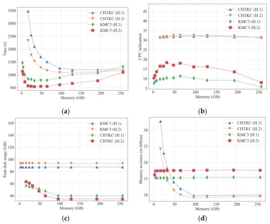
Figure 1.
Comparison of KMC3 and CHTKC with various memory limits for counting 32-mer in H.1 and H.2. (a) running time; (b) CPU utilization rate; (c) peak disk consumption; (d) memory access times.
When the available memory changes, there is no significant difference in the two indices of branch prediction and cache miss, indicating that the logic of the two algorithms is reliable (Supplementary Table S1). Therefore, we will not discuss the two indices later. Both KMC3 and CHTKC benefit from the scale of available memory, though KMC3 outperforms CHTKC on both H.1 and H.2 datasets (Figure 1a). KMC3 using 8 GB RAM has an unexpectedly shorter running time than CHTKC with 16 GB RAM. When the available memory exceeds 16 GB, the performance of KMC3 does not improve with the increase in the available memory. Instead, the memory management mechanism of the Linux system reduces its IO efficiency, resulting in performance degradation. More available memory enables CHTKC to build a larger hash table to accommodate more k-mers, reduces the super k-mers that need to transfer to disk, and dramatically lowers time consumption. CHTKC has the minimum disk usage and the optimal performance when the available memory reaches 96 GB. After that, the algorithm performance of CHTKC is no longer improved with more available memory and is even slightly degraded due to the mechanism of the Linux system. Overall, memory capacity is the key to the NPBKMC algorithm.
Since k-mer frequency counting is not a compute-intensive task, both algorithms cannot fully utilize the CPU (Figure 1b). The CPU utilization of the CHTKC algorithm is slightly higher than that of KMC3 due to the hash function calculation bringing extra computational complexity. Figure 1a–d show that the running time of CHTKC correlates with IO and memory access. When the available memory is less than 96 GB, CHTKC needs to write some k-mers to disk and triggers more cache replacements in the k-mer counting of H.1 and H.2, resulting in frequent cache load/store operations. When the number of distinct k-mers far exceeds the capacity of the hash table, CHTKC has multiple data exchanges between memory and disk, resulting in performance degradation. For example, H.1 is smaller than H.2, but H.1 has more k-mers in total and more distinct k-mers than H.2 due to the sequencing quality. CHTKC requires 2, 3, and 4 batches of memory and disk exchanges when the ratio of the number of distinct k-mers to the number of total k-mers reaches 0.16, 0.33, and 0.5. When the ratio is 0.5, the running time is near six times as long as the ratio is 0.11 (Supplementary Table S2). In summary, CHTKC is sensitive to the number of distinct k-mers.
3.2. Influence of IO Bandwidth
To assess the influence of IO bandwidth on the algorithms, we counted 32-mers in H.1 with KMC3 and CHTKC on Server 2. We assigned 32 and 30 threads to CHTKC and KMC3 separately to balance computing power because the computing capability of Server 2 is relatively poor. We allocated 48 GB of memory to the two algorithms. These parameters are close to the upper bound of hardware. We hope to observe how the two algorithms are affected by IO factors after using memory as much as possible. All other parameters are set to the default value.
The experiment shows both KMC3 and CHTKC spend more time completing the counting task with smaller IO bandwidth (Figure 2). Among them, KMC3 is relatively more affected by IO conditions than CHTKC. For example, when the k-mer length is 32, the running time of KMC3 in storage A increases by 59% compared with storage B. Furthermore, the running time of CHTKC in storage A only increases by 4% compared with storage B. We inferred that KMC3 needs to perform data exchange between memory and disk regardless of the dataset size as a disk-based algorithm, resulting in KMC3 being IO bandwidth dependent. In contrast, the mechanism of using memory whenever possible makes CHTKC is less IO sensitive. Thus, we are convinced CHTKC as an NPBKMC performs better than PBKMC when CHTKC is running in an environment with lower IO bandwidth and more available memory.
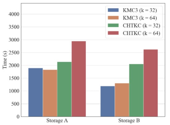
Figure 2.
Comparison of KMC3 and KMC3-R with different IO bandwidth.
Considering that disk-based partitioning is an IO-intensive operation, and the memory mode of KMC3 can eliminate the overhead of writing and re-reading partition results, we compared the disk mode of KMC3 with the memory mode of KMC3 (Figure 3). Figure 3a shows that the KMC3-R has better overall performance than KMC3, especially when the available memory is sufficient. Combined with Figure 1c, it can infer that the disk space that KMC3 in disk mode needs to consume does not correlate with the memory size. Furthermore, we evaluated the running time of each stage. Figure 3c shows that the partition (stage 1) performance degrades with increased memory.
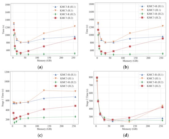
Figure 3.
Comparison of KMC3 and KMC3-R in counting 32-mer with various memory limits. KMC3-R: KMC3 with the memory mode. The running time of each stage is collected by timing in KMC3. (a) running time; (b) actually used memory; (c) running time of stage 1; (d) running time of stage 2.
In a Linux system, the running memory of a process consists of the memory directly requested and used by the process and the buffer cache used by the Linux system to optimize IO efficiency. When the process’s runtime memory allocated by the Linux system exceeds the free memory of the current system, the system will hijack the buffer cache to meet the requirement of the available memory of the process. As a result, the process performs direct IO more frequently, reducing the IO efficiency. Suppose the IO operations required in the partition stage of KMC3 remain unchanged, and the process requires a great deal of memory. In that case, it leads to worse IO efficiency in the partition stage. Considering that the counting stage needs to read the partition results from the disk, it also degrades the efficiency in the counting stage. Figure 3b–d demonstrate that the performance of partition and counting in memory mode does not degrade as much as disk mode if k-mers are in memory during the partition stage. To summarize, an IO-intensive operation such as disk-based partitioning does not benefit from requesting more memory but loses IO efficiency due to the decreasing buffer cache. Therefore, allocating excessive memory for large dataset k-mer counting tasks reduces the IO efficiency, especially the performance of the PBKMC job.
4. Influence of Dataset Features
In bioinformatics research, GC content, sequencing depth, and sequencing quality may affect sequencing data analysis. We evaluated the performance of the two algorithms by counting 32-mers of simulated sequencing datasets with various GC ratios (Figure 4), sequencing depths (Figure 5), and sequencing errors (Figure 6) on Server 1. The memory parameters of both algorithms are 128 GB. We assigned 32 (excluding reader and writer threads) and 34 threads to KMC3 and CHTKC separately. Other parameters are the default value.
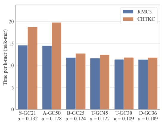
Figure 4.
Comparison of KMC3 and CHTKC using various GC-ratio datasets. α is the ratio of the number of distinct 32-mers to total 32-mers.
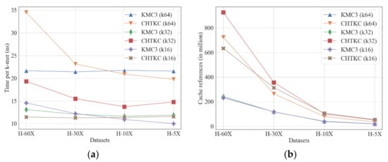
Figure 5.
Comparison of KMC3 and CHTKC with various sequencing depth. (a) running time; (b) cache reference.
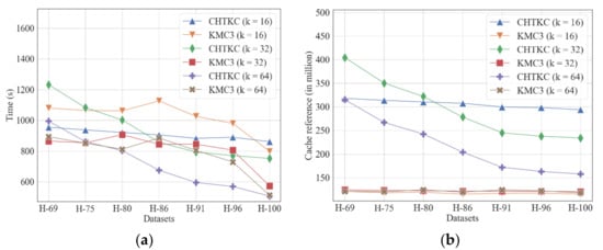
Figure 6.
Comparison of KMC3 and CHTKC with various sequencing errors. (a) running time; (b) cache reference.
4.1. Correlation of GC-Ratios
Our experiments show that the GC ratio does not significantly affect the performance of the two algorithms (Spearman test, p > 0.5 for both algorithms). However, the time consumption of both algorithms has a negative correlation with the ratio of the number of distinct k-mers and the total number of k-mers in the dataset (Spearman’s correlation, KMC3: r = −0.487, p = 0.006; CHTKC: r = −0.555, p =0.001). The larger the ratio, the more degraded algorithm performance is, and sequencing quality and dataset size are more easily affected (Figure 4). The above results show that we should optimize the k-mer counting algorithm according to the number of distinct k-mers and the total k-mers in the dataset. GC content cannot be used as an index to evaluate the algorithm’s robustness.
4.2. Influence of Sequencing Depths and K
Overall, KMC3 and CHTKC perform stably on datasets with various sequencing depths regardless of k-mer length, but KMC3 is more efficient for calculating long k-mers in large datasets with high sequencing coverage (Figure 5a, Supplementary Table S5). CHTKC has better competitive when dealing with low sequencing depth or short k-mers because the short k-mer or low sequencing depth counting tasks have a relatively small number of distinct k-mers (Table 3). CHTKC only needs 1–2 passes to complete these tasks when it has enough memory in this case. The case of counting long k-mer for high coverage sequencing data (k ≥ 32 and coverage ≥ 30x) means CHTKC must visit a large number of distinct k-mers and needs more batches to complete the task. More passes lead to more memory accesses (Figure 5b) and disk operations. More disk accesses imply the algorithm tends to be increasingly affected by the IO bottleneck, making it difficult to improve the performance. On the contrary, the partition-based KMC3 is related to the total k-mers, and the running time depends linearly on sequencing depth/number of total k-mers for each task with the same k-mer length.
4.3. Influence of Sequencing Quality
Our experiments show that for the three lengths of k-mer CHTKC is more sensitive to sequencing quality than KMC3 (Figure 6a). When the dataset has poor sequencing quality, sequencing errors dramatically increase the number of distinct k-mers. The k-mers generated by sequencing errors are low-frequency and random. For CHTKC, these k-mers can exhaust the pre-allocated hash table very soon. Afterward, the algorithm must save the following k-mers to disk, which may cause multiple batches of swaps between memory and disk, resulting in longer running time. Therefore, we can conclude that CHTKC as an NPBKMC algorithm is sensitive to the number of distinct k-mers.
Compared with the NPBKMC algorithm, KMC3 as a PBKMC algorithm is not so sensitive to the number of distinct k-mers, which gives it a significant advantage over the NPBKMC algorithm when dealing with frequency counting tasks of datasets with long k-mers and relatively low sequencing quality. Furthermore, the memory access of KMC3 relates to the number of total k-mers and does not linearly correlate with the number of distinct k-mers (Figure 6b). Nevertheless, the decrease in file size also decreases the time consumption of reading the Gzipped file, and KMC3 can also benefit from the decreasing of Gzipped file size with the improvement of sequencing quality, leading to less time consumption in the partition stage (Supplementary Table S7).
5. Scalability
Scalability reflects the influence of computing platform and input dataset size on algorithm delivery performance. Strongly scalable algorithms enable users to reduce computing time by increasing computing power. Weakly scalable algorithms imply that dataset size has little influence on the delivery performance of the algorithm. We evaluated the strong scalability of KMC3 and CHTKC by counting the 32-mers in H.1 and H.2, and the thread numbers start from 4 and double next time. We assessed the weak scalability by calculating three kinds of k-mer, in which we doubled the dataset H-86 and thread numbers simultaneously. The memory constraint parameters of both algorithms are 128 GB. KMC3 has two fewer threads than CHTKC because KMC3 automatically activates extra reader and writer threads. Other parameters are the default value. All tests are conducted on Server 1.
5.1. Strong Scalability
CHTKC achieves ideal speedup on both H.1 and H.2 in the strong scalability test (Figure 7 and Supplementary Table S8). In contrast, the speedup ratio of KMC3 tends to remain unchanged after the thread number exceeds 8, which shows relatively poor strong scalability. Since CHTKC’s hash function calculation is more computationally expensive than the partitioning and counting scheme of KMC3, more threads can speed up the lookup of the hash table. Because CHTKC adopts a chain hash table and lock-free CAS operation, the negative effect of race condition among threads is limited and does not limit the strong scalability. On the contrary, the low CPU utilization of KMC3 indicates the computational resources are not the bottleneck (Figure 1b), and more threads do not significantly contribute to the strong scalability. In addition, the limited scalability of the Raduls algorithm restricts the KMC3 algorithm cannot have better scalability. Since the impact of IO on the KMC3 algorithm is more noticeable, the strong scalability of KMC3 is relatively poor. Overall, KMC3 relies less on computing power, whereas CHTKC can make better use of computing resources.
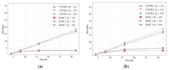
Figure 7.
Strong scalability comparison of KMC3 and CHTKC. (a) counting k-mers with various lengths in H.1; (b) counting k-mers with various lengths in H.2.
5.2. Weak Scalability
CHTKC and KMC3 show two opposite trends in the test of weak scalability when the dataset size and the number of threads increase proportionally (Figure 8 and Supplementary Table S9). The running time of KMC3 increases when the dataset size and thread number double simultaneously, indicating that KMC3 is not weakly scalable, so KMC3 cannot take advantage of the multi-core computing platform when processing large datasets. On the contrary, the running time of CHTKC decreases with the increase in dataset, indicating that CHTKC is weakly scalable, hence CHTKC is very suitable for k-mer frequency counting of super-scale datasets on high-performance computing platforms.
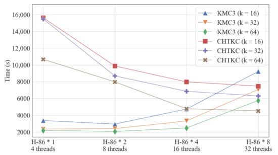
Figure 8.
Weak scalability comparison of KMC3 and CHTKC.
6. Optimization of PBKMC Algorithm
The above sections show that disk IO is a bottleneck of PBKMC and NPBKMC algorithms, indicating decreasing the disk access is critical to improving the delivery performance of the algorithms. Previous research showed that the frequency of each distinct k-mer in the sequencing data conforms to the Zipfian distribution []. That is, the vast majority of k-mers are often low-frequency in a sequencing dataset, and most of them only appear only once. Further analysis showed that the ratio of singleton k-mers that only appeared once to all distinct k-mers positively correlates with the k-mer length. We found that 21.9% distinct 16-mers, 77.1% of distinct 32-mers, and 77.2% distinct 64-mers in H.1 are singleton k-mers. Obviously, we can omit the frequency of a singleton k-mer. If a frequency-aware algorithm can optimize the processing flow of many singleton k-mers in sequencing data, alleviating the influence of the IO bottleneck is possible.
Meanwhile, two adjacent k-mers from a DNA sequence share k-1 bases. The k-mers caused by sequencing errors are more likely to be singletons, and every sequencing error may generate k consecutive singletons at most. This spatial correlation can significantly reduce the memory and disk resources required for the algorithm, thereby lowering the influence of the IO bottleneck.
To verify our observation, we revised KMC3 with the above idea and kept the inherent advantages of the KMC3 algorithm to reduce memory and disk usage significantly.
6.1. Optimizing Disk IO with an Overlapping Sequence Set
We improved the KMC algorithm by filtering and gluing the first-occurring k-mers to decrease disk occupation (Figure 9). First, the DNA sequence data are read into the memory in the partition stage through the reader thread and then passed to the worker threads through a blocking queue. Next, the worker threads divide the DNA sequences into k-mers and transmit each k-mer to a bloom filter to check if the k-mer is the first occurrence. The consecutive first-occurring k-mers are merged into an overlapping sequence, and non-first-occurring k-mers are distributed according to the process of KMC3. The overlapping sequences are also distributed to the corresponding overlapping sequence sets according to the partitioning rules consistent with KMC3 and written into different files. As a result, every partition in our algorithm has two files: one for the overlapping sequence set we produced and the other for the super k-mers used in the counting stage. After that, the counting stage of the revised algorithm is consistent with the counting stage of KMC3.
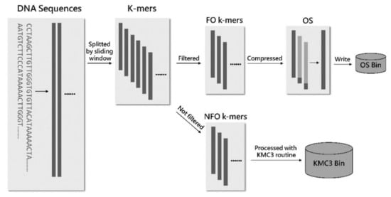
Figure 9.
The partition procedure of the revised KMC3 algorithm. FO k-mers denote first-occurring k-mers, NFO k-mers denote non-first-occurrence k-mers, and OS denotes overlapping sequence.
By introducing a bloom filter to filter the first occurrence of k-mers and storing them as overlapping sequences, singleton k-mers that occupy most of the input data are stored on disk in a highly compact manner. Therefore, the spatial correlation of k-mers described above is effectively utilized, and the IO performance can be significantly optimized. It also prevents many singleton k-mers from using extra memory in the subsequent counting stage, which improves the overall efficiency of the algorithm from another perspective.
We evaluated the improved algorithm using simulated sequencing datasets (Table 6). When k = 32, the singleton k-mers in the sequencing data make up the majority, the revised KMC3 algorithm only needs nearly half of the disk space of other algorithms with similar running memory, which suggests a significant optimization in disk access. As a result, the revised KMC3 algorithm is slightly faster than others when processing large datasets. The improved KMC3 algorithm performs better when k is larger. For example, the improved KMC3 algorithm is 13% faster than CHTKC and 18% faster than KMC3 in T-GC45, a dataset with more than 9 GB input. With the increase in dataset size, the advantage of the revised algorithm in terms of IO becomes more apparent. When counting the 64-mer frequency of H-GC41 in the same memory space, the running time of the improved algorithm is nearly five times faster than CHTKC and 33% faster than KMC3. Our experiments show that the revised algorithm has excellent performance when dealing with large datasets and frequency counting tasks with larger k-mers. Because sequencing errors result in more singleton k-mers, the revised algorithm has an increasing advantage over low sequencing quality data (Figure 10).
Table 6.
Comparison of KMC3, CHTKC, and Revised KMC3 with various sequencing data (Memory quota 16 GB).
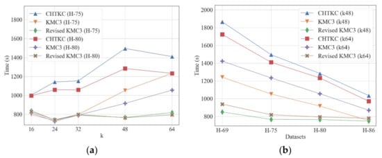
Figure 10.
Comparison of KMC3, CHTKC, and Revised KMC3 with various sequencing errors. Memory quota: CHTKC 128 GB, KMC3 32 GB, and Revised KMC3 32 GB. (a) counting tasks with various k; (b) counting tasks in various datasets.
6.2. Optimizing K-Mer Dumping with Read-Write Separation
Usually, k-mer frequency counting algorithms do not directly output the frequency counting results to the disk in text format but write the results in binary encoding format. The binary result file is generally smaller than the input data file. To visit frequency files in text format, a decoder program independent of the frequency counting algorithm loads the result as needed.
Similar to the frequency counting algorithm, the decoding performance of both KMC3 and CHTKC decoding programs is limited mainly by the IO bottleneck. In the decoding program of KMC3, the reading, decoding, and outputting of the binary code are all completed by one thread. Each time a k-mer is decoded, a disk write is executed. This method means that the decoding of each k-mer needs to block and wait for the IO device to be ready for every single k-mer, which significantly limits the overall throughput of the decoding program.
We optimized the decoder program of KMC3 with a read-write separation strategy and combined it with the improved KMC3 algorithm to reduce the IO overhead. The optimized decoder program reads the binary encoded file in blocks and decodes k-mer frequency pairs using the reader thread. Then, the reader thread submits the decoded blocks to the writer thread through a block queue, and the writer thread performs the actual disk writing operation. By separating the reader thread and the writer thread, the decoding operation performed by the reader thread does not need to wait to complete disk writing. The next round of reading and decoding can start immediately after the decoded result is submitted to the queue. Our decoding program demonstrated better performance in evaluations using simulated sequencing datasets than other dump programs (Figure 11). The experiments show that the revised algorithm dumps its counting results 8–60% faster than CHTKC and 3–6% faster than KMC3.
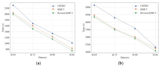
Figure 11.
Comparison of the dumper of KMC3, CHTKC, and Revised KMC3 with various sequencing data. (a) k = 32; (b) k = 64.
7. Conclusions
We comprehensively evaluated KMC3 and CHTKC, the representative partition-based k-mer counting algorithm and non-partition-based k-mer counting algorithm, to determine the type of computing task suitable for them and the breakthrough point for further optimization. From the dimension of hardware setting, KMC3 is the best choice for large datasets in the case of small memory (less than 64 GB) and high IO bandwidth (using SSD or RAID0). From the dimension of dataset features, KMC3 is better at processing datasets with long k-mers (k > 24) and relatively low sequencing quality (Q30 < 90%), and CHTKC is good at counting short k-mers in relatively high sequencing quality datasets. In addition, CHTKC is more efficient for calculating the k-mer frequency of super-scale datasets on high-performance computing platforms.
No matter which algorithm is involved, we cannot improve the performance anymore after the memory allocated for the algorithm reaches an upper bound. Moreover, the occupation of the buffer cache by memory allocation degrades the IO performance. Therefore, reducing the influence of the IO bottleneck is an inevitable step for optimizing the k-mer counting algorithm. We verified our judgment by filtering and compressing the consecutive first-occurring k-mers to reduce the number of disk access. However, the revision only targets large datasets or low sequencing quality datasets currently, and building a filtering method that is insensitive to the dataset is still a challenge. We also found almost all k-mer counting algorithms are platform-sensitive, and no algorithm is always highly efficient on arbitrary servers. In the future, we will continue to investigate strategies that can alleviate the influence of IO bandwidth. We will also develop self-configured k-mer counting tools to solve the platform-sensitive issues.
Supplementary Materials
The following supporting information can be downloaded at: https://www.mdpi.com/article/10.3390/a15040107/s1, Table S1: Comparison of KMC3 and CHTKC with various memory limit for H.1 and H.2 (k = 32); Table S2: CHTKC’s correlation between the running time and the ratio of the number of distinct k-mers to the number of total k-mers. The total k-mers is set to 1 billion; Table S3: Comparison of KMC3 and KMC3-R with various memory limit (k = 32); Table S4: Comparison of KMC3 and CHTKC using various GC-ratio datasets; Table S5: Comparison of KMC3 and CHTKC with various sequencing depth; Table S6: Comparison of KMC3 and CHTKC with various sequencing errors; Table S7: Comparison of the time usage of different stages of KMC3 with various sequencing errors; Table S8: Strong scalability comparison of KMC3 and CHTKC; Table S9: Weak scalability comparison of KMC3 and CHTKC; Table S10: Comparison of the dumper of KMC3, CHTKC and Revised KMC3 with various sequencing errors.
Author Contributions
Data curation, J.L.; Methodology, D.T. (Deyou Tang); Software, D.T. (Daqiang Tan) and W.X.; Supervision, D.T. (Deyou Tang); Validation, W.X.; Writing—Original draft, D.T. (Daqiang Tan); Writing—Review and editing, D.T. (Deyou Tang) and J.F. All authors have read and agreed to the published version of the manuscript.
Funding
This work was funded by the National Key R&D Program of China [2018YFC0910200].
Institutional Review Board Statement
Not applicable.
Informed Consent Statement
Not applicable.
Data Availability Statement
Not applicable.
Acknowledgments
The authors would like to thank Pingjian Zhang and Hu Chen for their valuable suggestions, and Yuchen Li for interface implementation.
Conflicts of Interest
The authors declare no conflict of interest.
References
- Chor, B.; Horn, D.; Goldman, N.; Levy, Y.; Massingham, T. Genomic DNA k-mer spectra: Models and modalities. Genome Biol. 2009, 10, R108. [Google Scholar] [CrossRef] [PubMed] [Green Version]
- Audoux, J.; Philippe, N.; Chikhi, R.; Salson, M.; Gallopin, M.; Gabriel, M.; Le Coz, J.; Drouineau, E.; Commes, T.; Gautheret, D. DE-kupl: Exhaustive capture of biological variation in RNA-seq data through k-mer decomposition. Genome Biol. 2017, 18, 243. [Google Scholar] [CrossRef] [PubMed]
- Deorowicz, S. FQSqueezer: K-mer-based compression of sequencing data. Sci. Rep. 2020, 10, 578. [Google Scholar] [CrossRef] [PubMed] [Green Version]
- Nasko, D.; Koren, S.; Phillippy, A.; Treangen, T.J. RefSeq database growth influences the accuracy of k-mer-based lowest common ancestor species identification. Genome Biol. 2018, 19, 165. [Google Scholar] [CrossRef] [Green Version]
- Cserhati, M.; Xiao, P.; Guda, C. K-mer-Based Motif Analysis in Insect Species across Anopheles, Drosophila, and Glossina Genera and Its Application to Species Classification. Comput. Math. Methods Med. 2019, 2019, 4259479. [Google Scholar] [CrossRef]
- Han, G.-B.; Cho, D.H.O. Genome classification improvements based on k-mer intervals in sequences. Genomics 2019, 111, 1574–1582. [Google Scholar] [CrossRef]
- Jaillard, M.; Lima, L.; Tournoud, M.; Mahé, P.; Van Belkum, A.; Lacroix, V.; Jacob, L. A fast and agnostic method for bacterial genome-wide association studies: Bridging the gap between k-mers and genetic events. PLoS Genet. 2018, 14, e1007758. [Google Scholar] [CrossRef] [Green Version]
- Kurtz, S.; Narechania, A.; Stein, J.C.; Ware, D. A new method to compute K-mer frequencies and its application to annotate large repetitive plant genomes. BMC Genom. 2008, 9, 517. [Google Scholar] [CrossRef] [Green Version]
- Marcais, G.; Kingsford, C. A fast, lock-free approach for efficient parallel counting of occurrences of k-mers. Bioinformatics 2011, 27, 764–770. [Google Scholar] [CrossRef] [Green Version]
- Melsted, P.; Pritchard, J. Efficient counting of k-mers in DNA sequences using a bloom filter. BMC Bioinform. 2011, 12, 333. [Google Scholar] [CrossRef] [Green Version]
- Deorowicz, S.; Debudaj-Grabysz, A.; Grabowski, S. Disk-based k-mer counting on a PC. BMC Bioinform. 2013, 14, 160. [Google Scholar] [CrossRef] [PubMed] [Green Version]
- Deorowicz, S.; Kokot, M.; Grabowski, S.; Debudaj-Grabysz, A. KMC 2: Fast and resource-frugal k-mer counting. Bioinformatics 2015, 31, 1569–1576. [Google Scholar] [CrossRef] [Green Version]
- Kokot, M.; Długosz, M.; Deorowicz, S. KMC 3: Counting and manipulating k-mer statistics. Bioinformatics 2017, 33, 2759–2761. [Google Scholar] [CrossRef] [PubMed] [Green Version]
- Rizk, G.; Lavenier, D.; Chikhi, R. DSK: K-mer counting with very low memory usage. Bioinformatics 2013, 29, 652–653. [Google Scholar] [CrossRef] [PubMed]
- Roy, R.; Bhattacharya, D.; Schliep, A. Turtle: Identifying frequent k-mers with cache-efficient algorithms. Bioinformatics 2014, 30, 1950–1957. [Google Scholar] [CrossRef] [PubMed] [Green Version]
- Audano, P.; Vannberg, F. KAnalyze: A Fast Versatile Pipelined K-mer Toolkit. Bioinformatics 2014, 30, 2070–2072. [Google Scholar] [CrossRef] [PubMed] [Green Version]
- Kaplinski, L.; Lepamets, M.; Remm, M. GenomeTester4: A toolkit for performing basic set operations-union, intersection and complement on k-mer lists. Gigascience 2015, 4, 58. [Google Scholar] [CrossRef] [Green Version]
- Crusoe, M.R.; Alameldin, H.F.; Awad, S.; Boucher, E.; Caldwell, A.; Cartwright, R.; Charbonneau, A.; Constantinides, B.; Edvenson, G.; Fay, S.; et al. The khmer software package: Enabling efficient nucleotide sequence analysis. F1000Research 2015, 4, 900. [Google Scholar] [CrossRef] [Green Version]
- Mamun, A.-A.; Pal, S.; Rajasekaran, S. KCMBT: A k-mer Counter based on Multiple Burst Trees. Bioinformatics 2016, 32, 2783–2790. [Google Scholar] [CrossRef] [Green Version]
- Erbert, M.; Rechner, S.; Müller-Hannemann, M. Gerbil: A fast and memory-efficient k-mer counter with GPU-support. Algorithms Mol. Biol. 2017, 12, 9. [Google Scholar] [CrossRef] [Green Version]
- Wang, J.; Chen, S.; Dong, L.; Wang, G. CHTKC: A robust and efficient k-mer counting algorithm based on a lock-free chaining hash table. Brief. Bioinform. 2021, 22, bbaa063. [Google Scholar] [CrossRef] [PubMed]
- Tang, D.; Li, Y.; Tan, D.; Fu, J.; Tang, Y.; Lin, J.; Zhao, R.; Du, H.; Zhao, Z. KCOSS: An ultra-fast k-mer counter for assembled genome analysis. Bioinformatics 2022, 38, 933–940. [Google Scholar] [CrossRef] [PubMed]
- Marchet, C.; Kerbiriou, M.; Limasset, A. BLight: Efficient exact associative structure for k-mers. Bioinformatics 2021, 37, 2858–2865. [Google Scholar] [CrossRef] [PubMed]
- Purcell, C.; Harris, T. Non-blocking Hashtables with Open Addressing. In Proceedings of the Distributed Computing, International Conference, DISC, Cracow, Poland, 26–29 September 2005. [Google Scholar]
- Steffen, H.; Justin, Z.; Hugh, E.W. Burst tries: A fast, efficient data structure for string keys. ACM Trans. Inf. Syst. 2002, 20, 192–223. [Google Scholar]
- Li, Y.; Yan, X. MSPKmerCounter: A Fast and Memory Efficient Approach for K-mer Counting. arXiv 2015, arXiv:1505.06550. [Google Scholar]
- Kokot, M.; Deorowicz, S.; Debudaj-Grabysz, A. Sorting Data on Ultra-Large Scale with RADULS. In International Conference: Beyond Databases, Architectures and Structures, Proceedings of the 13th International Conference, BDAS 2017, Ustroń, Poland, 30 May–2 June 2017; Springer: Cham, Switzerland, 2017; Volume 716, pp. 235–245. [Google Scholar]
- Manekar, S.C.; Sathe, S.R. A benchmark study of k-mer counting methods for high-throughput sequencing. Gigascience 2018, 7, giy125. [Google Scholar] [CrossRef] [Green Version]
- Pandey, P.; Bender, M.A.; Johnson, R.; Patro, R. Squeakr: An exact and approximate k-mer counting system. Bioinformatics 2018, 34, 568–575. [Google Scholar] [CrossRef]
- Pandey, P.; Bender, M.A.; Johnson, R.; Patro, R. A General-Purpose Counting Filter: Making Every Bit Count. In Proceedings of the 2017 ACM International Conference on Management of Data, Association for Computing Machinery, Chicago, IL, USA, 9 May 2017; pp. 775–787. [Google Scholar]
- Pérez, N.; Gutierrez, M.; Vera, N. Computational Performance Assessment of k-mer Counting Algorithms. J. Comput. Biol. 2016, 23, 248–255. [Google Scholar] [CrossRef]
- Xiao, M.; Li, J.; Hong, S.; Yang, Y.; Li, J.; Wang, J.; Yang, J.; Ding, W.; Zhang, L. K-mer Counting: Memory-efficient strategy, parallel computing and field of application for Bioinformatics. In Proceedings of the 2018 IEEE International Conference on Bioinformatics and Biomedicine (BIBM), Madrid, Spain, 3–6 December 2018; pp. 2561–2567. [Google Scholar]
- Liu, B.; Shi, Y.; Yuan, J.; Hu, X.; Zhang, H.; Li, N.; Li, Z.; Chen, Y.; Mu, D.; Fan, W. Estimation of genomic characteristics by analyzing k-mer frequency in de novo genome projects. arXiv 2013, arXiv:1308.2012. [Google Scholar]
- Li, R.; Fan, W.; Tian, G.; Zhu, H.; He, L.; Cai, J.; Huang, Q.; Cai, Q.; Li, B.; Bai, Y.; et al. The sequence and de novo assembly of the giant panda genome. Nature 2010, 463, 311–317. [Google Scholar] [CrossRef] [Green Version]
- Hu, X.; Yuan, J.; Shi, Y.; Lu, J.; Liu, B.; Li, Z.; Chen, Y.; Mu, D.; Zhang, H.; Li, N.; et al. pIRS: Profile-based Illumina pair-end reads simulator. Bioinformatics 2012, 28, 1533–1535. [Google Scholar] [CrossRef] [PubMed] [Green Version]
- Shokrof, M.; Brown, C.T.; Mansour, T.A. MQF and buffered MQF: Quotient filters for efficient storage of k-mers with their counts and metadata. BMC Bioinform. 2021, 22, 71. [Google Scholar] [CrossRef] [PubMed]
Publisher’s Note: MDPI stays neutral with regard to jurisdictional claims in published maps and institutional affiliations. |
© 2022 by the authors. Licensee MDPI, Basel, Switzerland. This article is an open access article distributed under the terms and conditions of the Creative Commons Attribution (CC BY) license (https://creativecommons.org/licenses/by/4.0/).