A Methodology to Design Quantized Deep Neural Networks for Automatic Modulation Recognition

Abstract

Next-generation communication systems will face new challenges related to efficiently managing the available resources, such as the radio spectrum. DL is one of the optimization approaches to address and solve these challenges. However, there is a gap between research and industry. Most AI models that solve communication problems cannot be implemented in current communication devices due to their high computational capacity requirements. New approaches seek to reduce the size of DL models through quantization techniques, changing the traditional method of operations from a 32 (or 64) floating-point representation to a fixed point (usually small) one. However, there is no analytical method to determine the level of quantification that can be used to obtain the best trade-off between the reduction of computational costs and an acceptable accuracy in a specific problem. In this work, we propose an analysis methodology to determine the degree of quantization in a DNN model to solve the problem of AMR in a radio system. We use the Brevitas framework to build and analyze different quantized variants of the DL architecture VGG10 adapted to the AMR problem. The evaluation of the computational cost is performed with the FINN framework of Xilinx Research Labs to obtain the computational inference cost. The proposed design methodology allows us to obtain the combination of quantization bits per layer that provides an optimal trade-off between the model performance (i.e., accuracy) and the model complexity (i.e., size) according to a set of weights associated with each optimization objective. For example, using the proposed methodology, we found a model architecture that reduced 75.8% of the model size compared to the non-quantized baseline model, with a performance degradation of only 0.06%.

1. Introduction

Next-generation wireless communications are geared towards versatility and adaptability to different radio environments and channel dynamics. CR is an enabling technology that extends the functionality of SDR by providing the mechanism to adapt intelligently to its environment [1].

One of the critical features of CR is DSA, which allows radios to access and use the unused spectrum dynamically [2]. DSA involves several tasks that a radio should execute to improve its performance automatically. Among these tasks, AMR is one of the most studied in the literature [1,3,4]. One of the main challenges in AMR is to classify a received signal into a modulation type without (or with limited) prior information about the transmitted signal under dynamic channel conditions [5].

Traditionally, AMR has been mainly tackled via LB and expert FB methods combined with pattern recognition methods [6]. While LB methods find optimal solutions by minimizing the probability of false classification at the cost of high computational complexity, FB methods have lower complexity, and their performance is (near-)optimal when appropriately designed. However, these features are usually chosen by an expert and are based on a specific set of assumptions that are typically unrealistic [5]. In recent years, some limitations of such techniques have been solved by applying DL techniques such as DNN, which allow both automatically extracting the relevant features from raw time-series data and performing the classification task [7] on the extracted features.

More recently, several approaches based on DL have been proposed to solve the AMR task using raw time, frequency, and time-frequency data, outperforming traditional methods [5,7,8,9]. However, the primary assumption when using such models is the availability to train and run such models on high-end computational devices with hardware accelerators [10,11]. While this can be acceptable on traditional deployments where the radio is co-allocated with dedicated high-end servers, this is not the case for new approaches such as the desegregated RAN [12] for private deployments in dense environments. In such cases, DL models trained in the cloud/core network will not be able to run on the DU or RU of such desegregated RAN, since such components are intended to run at the edge or far edge, where computational resources are constrained and shared. Therefore, there is a clear need to adapt models trained in high-end devices such that they can run on constrained ones by trading performance (e.g., classification accuracy) against model complexity (e.g., model size) [13].

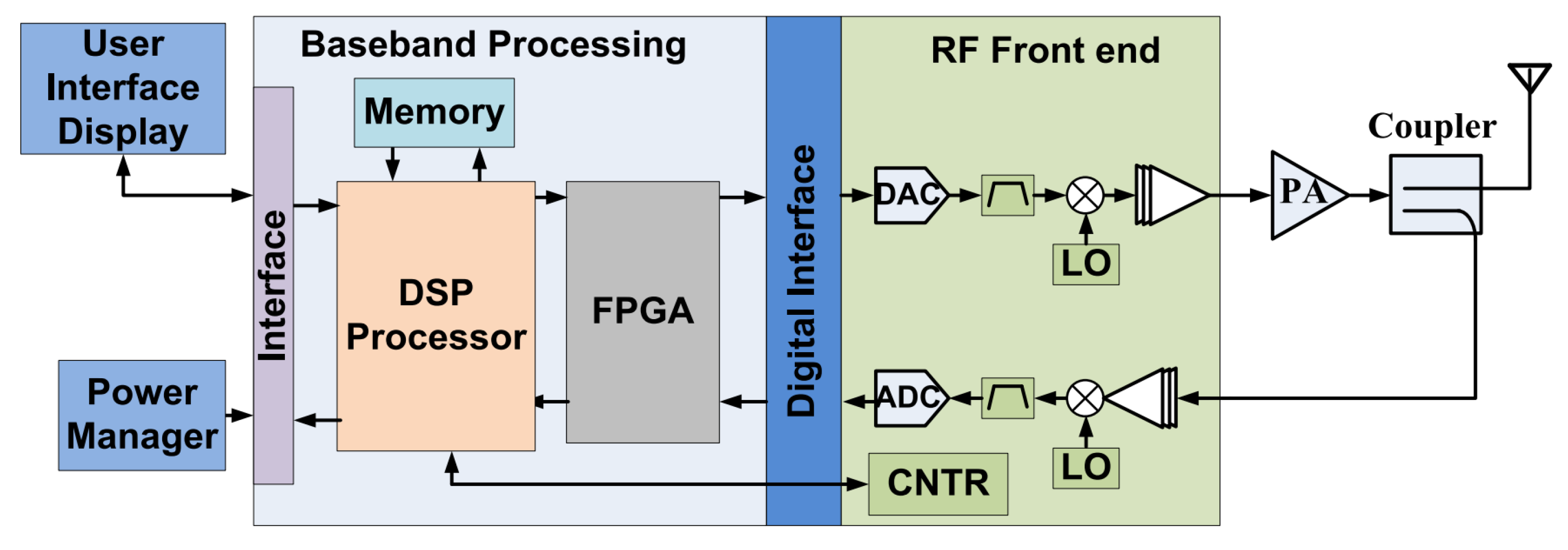
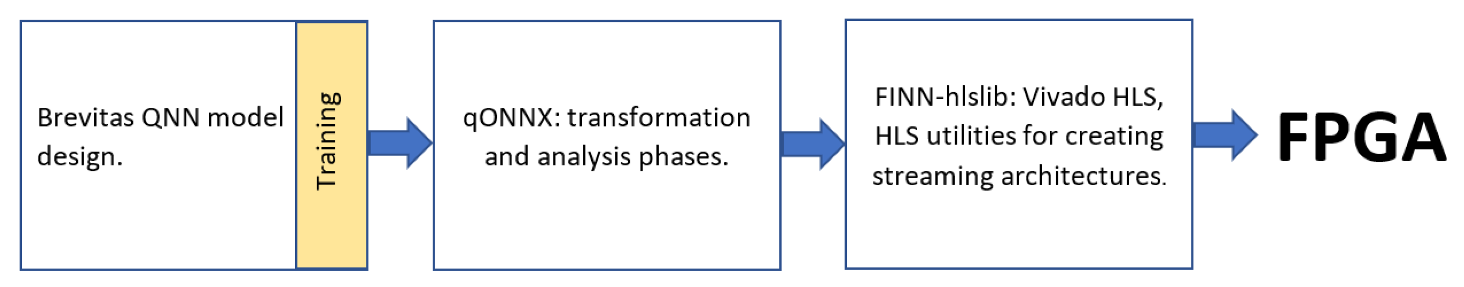
Recently, several frameworks and tools have been proposed to decrease the computational complexity of DNN using techniques such as quantization. Quantization reduces the models’ size by truncating the value of parameters such as inputs, activations, and weights. This truncation is achieved by moving from floating-point precision (e.g., 32 or 64 bits) representation of such parameters to a more straightforward and reduced representation using fewer bits as integers (e.g., 2, 4, and 8 bits). The main computational argument for quantization is that quantized weights and activations occupy much less memory space while trading-off model performance. The resulting quantized model can be housed entirely in the FPGA of the SDR device, allowing signal processing tasks, including DL-based ones, to be performed close to the radio. In addition, power consumption is reduced due to the simplification of the process by not having to work with floating-point modules [14].

The available literature on how to design, implement, and evaluate the performance of quantized DL for AMR is very limited [13,15]. Most of these works focus on the performance of the proposed DL model when all layers are quantized with the same quantization value. As a result, there are no methodologies or guidelines to design quantized DL models where the designer can trade-off both main optimization objectives, the models’ performance (e.g., accuracy) against the model complexity (e.g., model size). This trade-off is fundamental since different computational environments will provide different computing capabilities, and it is up to the designer to find a balance between both objectives.

In this paper, we propose a methodology based on statistical analysis and its related algorithms to determine the degree of quantization that is required to achieve a given trade-off between model performance and model complexity and, without loss of generality, we validate the proposed approach in a well-known DNN architecture that has been used for AMR. To the best of the authors’ knowledge, this is the first work that proposes a methodology that allows the design of quantized DL models for AMR with a given trade-off between accuracy and model complexity. The main contributions of this paper are twofold:

• We determine the strength of the relationship between the trainable parameters of a DNN architecture and objectives such as model performance (i.e., accuracy) and inference cost (related to model size).
• We provide a method of analysis to determine the degree of quantification that is required in each layer to achieve the desired trade-off between both objectives.

The rest of the paper is organized as follows. Section 2 introduces some terminology and background related to quantization in DNN. Section 3 presents the related work on quantized and non-quantized DNN for AMR. Section 4 shows the experimental methodology used to determine the relationship between the parameters quantified in the DL model and the optimization objectives to trade-off. Section 5 presents the experimental analysis of the effect of inputs, activation, and quantified weights on the performance and size of a well-known DL model (VGG10 1D-CNN) that has been used for AMR using the methodology proposed in the previous section. In addition, we present the related algorithms that support the methodology and can find model architectures that trade-off the optimization objectives. Finally, Section 6 concludes the paper and outlines future work in this research.

2. Background

Hardware accelerators have been a topic of interest in recent years, especially with the possibility of designing DL architectures that can be implemented on these devices. In the field of communications, the interest is mainly focused on the possibility of deploying DL algorithms as close as possible to the radio. For example, Figure 1 shows an SDR radio system’s schematic with different processing stages in which an FPGA is used as a hardware accelerator.

The FPGA is flexible enough to accommodate different DL models due to its reprogrammable architecture; that is, the FPGA can be reprogrammed according to the problem to be solved. However, the available computing resources on an FPGA are limited, and, therefore, DL algorithms have to be designed with those constraints in mind. More precisely, the traditional approach of training DL models on the cloud and directly deploying them on the radio is not suitable anymore. The main reason is that DL models are large, i.e., they usually contain millions of single-precision (FLOAT32) or double-precision (FLOAT64) floating-point trainable parameters and use a large amount of training data to achieve high performance in terms of accuracy. In order to remove such limitation, it is necessary to adapt such large DL models so that they can be deployed on the resource-constrained FPGA to perform the inference.

2.1. Quantization

Quantization is a mapping operation between a real value r and an integer value. Quantization reduces the numerical precision of a value in bit-width, or what is the same, to reduce the number of bits used to represent a number. In the case of CNN, reducing the bit-width representation in inputs, activations, and weights results in a model that requires less memory space. In symmetric quantization, Equation (1) defines the clip range in which the real value is mapped to the integer value using q-bit quantization.

$$(-s,+s)=(-2^{q-1}+1,2^{q-1}-1)$$

(1)

Once the limits of the clipping range are defined, the second step is to map the full-scale range of floating-point values to a range of integer format values by defining a threshold, as indicated in Equation (2). Then, positive values of the input are mapped to positive values of the integer representation.

$$IN{T}_{threshold}=\left\{\begin{array}{cc}+s\hfill & \mathrm{if}{r}_{Value}>0\hfill \\ -s\hfill & \mathrm{if}{r}_{Value}<0\hfill \end{array}\right.$$

(2)

Then, scale of the quantization is defined as shown in Equation (3), where $Valu{e}_{range}=[r_{max},r_{min}]$.

$$Scale=\frac{Valu{e}_{range}}{IN{T}_{threshold}}$$

(3)

Finally, the quantified value is as follows:

$$r_{INT}=\frac{r_{FLOAT}}{Scale}$$

(4)

2.2. Quantization Frameworks

The two most common frameworks that already provide functionalities to quantize for quantizing DL models are Tensorflow and Pytorch. These frameworks aim to quantize DL models that can run on resource-constrained CPU- or GPU-based hardware. However, these frameworks do not support FPGA-type hardware accelerators. On the other hand, Brevitas is a new Pytorch library for designing QNN models with different extraction levels that can be deployed to Xilinx FPGA via the experimental framework FINN [14].

Table 1. The table above gives us a general idea of the frameworks for quantized neural networks.

Frameworks	Technique	Supported Hardware
TensorFlow Quantization	Post-training float16 quantization Post-training dynamic range quantization Post-training integer quantization Quantization-aware training	CPU, GPU CPU, GPU (Android) CPU, GPU (Android), EdgeTPU, Hexagon DSP CPU, GPU (Android), EdgeTPU, Hexagon DSP
Pytorch Quantization	Dynamic/weight only quantization Static quantization Dynamic quantization	x86 CPUs with AVX2 support or higher. ARM CPUs (mobile/embedded devices) NVidia GPU –> TensorRT through fx2trt.
PyTorch Brevitas	Quantization-aware training - Integer quantization - Binary quantization - Ternary quantization	FINN –> Xilinx FPGA

shows the currently most widely used quantization frameworks and the hardware they support.

Since the interest of our work is oriented to build DL models that can be run on devices with limited computing resources such as FPGA, we focus on the Brevitas framework as it is the only framework that allows the design, development, and execution of QNN in FPGA [14,17,18,19,20]. Figure 2 shows the workflow followed by Brevitas, where:

• The model is developed and trained using Brevitas since it allows designing QNNs with different quantization levels oriented to their deployment in FPGAs. One distinguishing factor of Brevitas is its ability to allow input features to be quantized. Quantizing the input features is an aspect to consider since it is a feature that is not implemented in other frameworks and provides one more source of additional reduction that counts a lot in very constraineddevices such as the FPGA.
• Once the model is trained, it is exported using the ONNX standard. ONNX enables DL models to be transformed into a portable format. This preliminary step is carried out to bring the DL model to specific hardware.
• Once the model is in a standard format, it can be translated into the FPGA logic by FINN, using the Finn-hlslib Vivado HLS FPGA library.

3. Related Work

AMR is a field of interest in CR and intelligent communication systems [21]. The possibilities offered by detecting and identifying modulations are extensive in resource management, shared spectrum, and security. Therefore, it is not a new topic, and classic methods such as LB and FB on distribution tests perform the detection with an acceptable degree of certainty [3]. However, many researchers have been interested in improving the results obtained with classical methods using AI. Research on DL applications has been promoted in all phases of the end-to-end communication model.

3.1. AMR

Numerous works have investigated DL architectures that seek to improve the ability to detect and classify modulations compared to traditional methods such as LB and FB [6]. DNN-based classifiers have overcome the performance of traditional methods and methods based on statistical ML [5]. Moreover, DNN [22], i.e., ANN with more than one layer between the input and the output layers, have shown the best performance without explicitly requiring an FB method to extract the features of the radio signal [5,7,8,9]. DNN architectures can perform both the feature extraction and the classification of the radio signals using a unique ANN. Authors in [5] showed that a DNN based on a CNN outperformed several expert FB methods using different classifiers. CNNs are ANNs that use convolution in place of general matrix multiplication in at least one of their layers [22]. The CNN achieved a rough accuracy of 87% across all the 11 types of modulated radio signals and SNR in the test dataset, and using only raw I/Q samples of modulated radio signals as input. Similarly, Shengliang et al. [8] proposed a CNN classifier for images generated after data conversion from raw I/Q samples to gray images. Again, improvements and better classification accuracy were achieved over cumulant and ML-based AMR algorithms.

The authors of [23] proposed a CNN architecture trained on the DeepSig dataset named RadioML Dataset 2018.01A, which has 24 modulation classes. The results indicated that the classification accuracy improves in the range of SNR from −4 dB to 20 dB. In [24], the authors proposed a method that uses I/Q samples to form images with the “Stockwell discrete orthonormal transform”. Another technique is to perform transformations on the input I/Q samples to find other types of characteristics of the signal. Furthermore, it is possible to combine models trained on different datasets for better performance, such as in [25], where two models from CNN were integrated into a single general model that allows more accurate classification of different modulations. However, this method is not computationally cheap since it does not use dimensionality reduction methods.

Instead of using CNN, authors in [26] proposed a DL architecture based on ENN for AMR in multipath fading channels. The proposed DNN is based on the natural logarithmic energy model. The proposed ENN uses three smaller DNNs, each trained to recognize the radio signal’s amplitude, phase, and frequency. The results showed that the proposed ENN has a higher probability of correct classification than traditional algorithms for classifying modulations within the same training sequence and SNR. In [27], a CNN and an LSTM were combined to create an HDMF. A DL-based AMR method employing SCF was introduced. In the proposed method, a DBN is applied for pattern recognition and classification with high accuracy, even in the presence of environmental noise. Recently, works such as [28,29,30] addressed the problem of AMR based on the design and implementation of new AI architectures with improved performance.

Other approaches focus on the preprocessing of the input signal, which allows highlighting features that would otherwise not be observed, reduced, or extracted. For example, using different input types, an SAE was evaluated in [31]. The I/Q samples, the centroids of the constellation points, obtained using a fuzzy C-means algorithm, and the high-order cumulants of the received samples were used as training inputs. Each autoencoder layer was trained using unsupervised learning followed by a softmax classifier. The results showed that the accuracy of the proposed architecture outperformed AMR methods using an LB classifier, cumulant-based genetic programming in combination with KNN classifiers, and DNN using cumulants and instantaneous PSD as the features. Finally, the authors in [32] proposed an alternative approach to extract relevant features for AMR in the preprocessing phase. The authors used a GNN for AMR. However, since the GNN is function-based, while the input signal is a signal in the time domain, a CNN is needed to extract the functions and build the graphs for the GNN.

3.2. AMR with Low Computational Cost

Although the results of modulation detection and classification using the DL techniques presented above are promising, integrating these kinds of algorithms at the radio side to perform the task in real time requires high-end devices due to the high computational cost [10,11]. This computational cost comes from the many floating-point operations that must be performed while performing inference. As a solution, compressing the DL models has the advantage of reducing the number of floating-point operations and, in some cases, replacing them with fixed-point functions to trade-off the accuracy/performance of the model against its complexity, i.e., its computational cost.

The main advantage of compressing DL models is that it allows their deployment on resource-constrained devices while increasing processing speed and improving energy efficiency. In the case of new-generation communications such as 5G-NR, DL algorithms running on DU (e.g., an INTEL NUC or an NVIDIA Jetson) or at the RU (e.g., an SDR), will need to be compressed to guarantee real-time operation on constrained devices such as the ones deployed at the edge or far-edge. These devices are at the other end of capabilities compared to the cloud/core network, where, traditionally, DL models are trained and run for other AI tasks.

To reduce the model’s complexity, two well-known approaches are used to compress DL models: the first is based on network pruning techniques, and the second is based on the quantization of the input parameters of the network. Although they are entirely different techniques, they can be used individually or in combination on the same model to improve results. Pruning is the process that searches and identifies the weights of connections among neurons in DL models [33] that are redundant or are not needed such that the drop in accuracy is minimal when they are eliminated [23].

Reducing computational cost through quantization is an entirely different process than pruning since it replaces floating-point operations with fixed-point operations. With this approach, the authors of [13] proposed a QNN model for AMR. The quantized model achieved a classification accuracy of 75% with a signal-to-noise ratio SNR of 10 dB, similar to an unquantized model. In [15], a more versatile approach was followed. The authors suggested combining pruning and quantization techniques to reduce the model size further. The authors used different quantization levels and found no suitable combination, as the results indicated that the accuracy degraded considerably. As a solution, the authors applied pruningtechniques to the quantized model. The results showed a reduced inference cost with a limited drop in accuracy.

While the literature on DL models for AMR is extensive, this is not the case for compression methods that allow such models to run on constrained devices such as those found at the edge or far edge. In addition, the few works that provide evaluation results on compressed models for AMR focus on the performance of a single model with all layers quantized with the same quantization value. Having the same quantization level for all the model’s layers limits the application of such results since they do not provide insight about how to design the model so that we can trade-off the accuracy and model size.

4. Design Methodology for Quantization Selection

As seen in previous sections, robust DL models are typically used.Nevertheless, due to the size/complexity of such models, signal processing must be performed in machines with high computational power, which is not the characteristic of the devices composing the radio access, edge, or far-edge networks. In Section 2, we saw how quantization helps to reduce the computational cost of implementing a robust DL model; however, in Section 3, we showed that only few works focus on quantization of DL models for radio signals. Moreover, we could verify that there is no general approach or methodology that guides researchers and radio practitioners in selecting the degree of quantization of a model DL to achieve a desired trade-off level between performance and the model’s complexity.

To start the description of the proposed methodology, let us consider an experiment with three design factors, where each element has three possible levels. Then, using a complete factorial design, we would need to run the same experiment $3^3-1=26$ times to determine which design factor impacts the response variable (i.e., the outcome) the most. Translating this small example to the field of DL model quantization, if we have three quantifiable parameters (e.g., the input, the activation layers, and the weights), each in the range of 1 to 32 bits, it gives ${32}^3-1=32,767$ possible combinations. Evaluating the impact of each parameter’s quantization level regarding the accuracy and inference cost is prohibitively time- and resource-consuming.

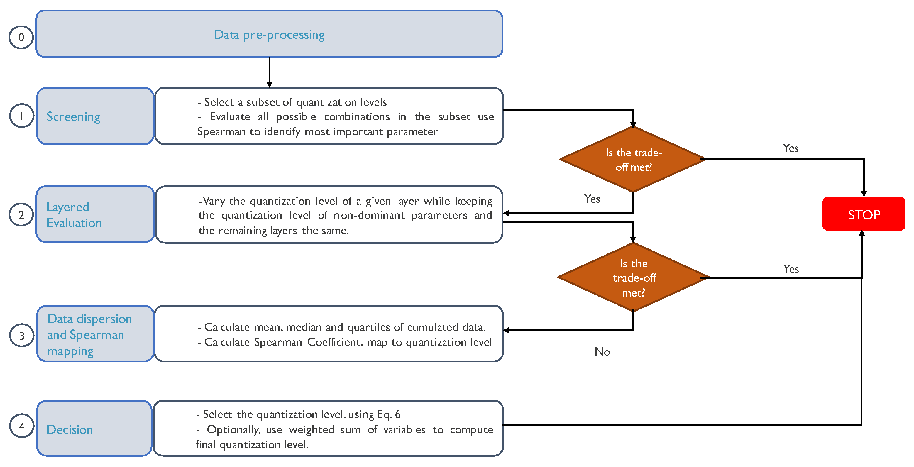
Based on a fractional factorial design [34], our methodology allows reducing the number of experiments concerning quantifiable parameters. We divide the methodology into four stages. After each stage, we measure the trade-off between the model’s performance metric (e.g., accuracy) and its inference cost (e.g., space in memory, number of operations) regarding the unquantized model. It is worth mentioning that it is possible to include a preprocessing of the input signals to reduce their size before applying this methodology, such as dimensionality-reduction methods or averaged filters. Figure 3 illustrates a detailed block diagram of the developed methodology.

During the first stage, we identify the dominant parameter in the quantization. To perform this, we select a subset of representative levels and evaluate all the possible combinations over that subset (i.e., screening). That evaluation is made regarding the model accuracy and the NICS (i.e., the outputs). Accuracy is the ratio between the number of correct and the total number of predictions in all classes. The NICS calculation is obtained by comparing the weight bits, total activation bits, and BOPS against the reference model, as described in Equation (5).

$$NICS=0.5\ast (bops/bop{s}_{baseline})+0.5\ast \left(w_{bits}/w_{bits\_baseline}\right)$$

(5)

where $bops$ and $bop{s}_{baseline}$ are the BOPS of the evaluated (quantized) and the reference (non-quantized) model, respectively. Similarly, $w_{bits}$ and $w_{bits\_baseline}$ are the total bits used by the weights in the evaluated and the reference models, respectively.

Note that previous information can help refine the selection of subsets. For instance, [35,36] showed that an 8-bit quantized CNN model achieves an accuracy close to that of an unquantized model for AMR. Then, a reduced subset of quantization levels can be used (i.e., from 1- to 8-bit quantization).

Once we obtain the performance and the inference cost for each combination of the subset, we apply Spearman’s correlation coefficient (see Equation (6)) to identify which quantized parameter (i.e., input, activations, and weights) has the highest impact on the output, i.e., the dominant parameter. We use Spearman’s correlation, where n is the number of observations and D is the variable of interest, since it allows for correlation variables that bear a nonlinear relationship. If, during the screening, a combination that meets the expected trade-off is found, e.g., by creating the Pareto front using the resulting accuracy and NICS metrics from the quantized models, then we can conclude our search. Otherwise, we can move to the second stage. Algorithm 1 shows the pseudocode of the first stage. Notice that the resulting accuracy and NICS metrics from the quantized models are returned in variable E in Algorithm 1.

$$\rho =1-\frac{6{\sum }_{i=1}^n{D}_i^2}{n\left(n^2-1\right)}$$

(6)

Algorithm 1 Screening: Detection of relevant parameters.

Require: I/Q samples data set $DS$.

Require: DNN model M.

Require: Set I with different number of bits to quantize the input parameter.

Require: Set a with different number of bits to quantize the activation function parameter on all layers.

Require: Set W with different number of bits to quantize the weight parameter on all layers.

1: Initialize set E of experiments

2: for $i\in I$ do

3:  Quantize M’s input with i bits

4:  for $a\in A$ do

5:    Quantize M’s activation functions with a bits

6:    for $w\in W$ do

7:      Quantize M’s weights with w bits

8:      Apply quantize-aware training to M and use dataset $DS$

9:      $Accurac{y}_{\{}i,a,w\}\leftarrow$ Calculate accuracy of M

10:      $NICS\{i,a,w\}\leftarrow$ Calculate NICS of M

11:      $Experiment\{i,a,w\}\leftarrow$ [$NICS\{i,a,w\}$, $Accurac{y}_{\{}i,a,w\}$]

12:      $E=E\cap Experiment\{i,a,w\}$

13:    end for

14:  end for

15: end for

16: Calculate Spearman’s correlation analysis on E

17: Return E and the parameter with higher correlation with respect to accuracy and NICS

Since modern DL models are composed of several layers, if the dominant parameters are activation or weights, we can evaluate in a layered way which layer has the highest effect on the trade-off (stage 2). Notice that the weights are more likely to significantly impact the accuracy and inference cost outputs compared to activations and inputs since there are more hidden units and connections among them than layers.

During the second stage, we measure the degree of quantization per layer required to meet a given trade-off. Notice that if the input is the parameter that most impacts the outputs, then the second stage is the same, but the only layer to alter is the input one. A good starting point is to take the same quantization subset as in stage one. In this stage, we vary the quantization level of a given layer while keeping the quantization level of the non-dominant parameters and the remaining layers the same.

Compared to previous works such as [13,15], our second stage differs from them since they typically apply the same quantization level to all the model’s layers. Suppose the trade-off between the model performance metric and the inference cost is met, then we conclude our search by obtaining an architecture in which we have identified which layer of the model has the highest impact. Otherwise, we can continue with the third stage. Algorithm 2 summarizes the procedure to analyze the effect of the quantization level in each layer of a DNN independently, assuming the weight parameter has the most impact in the output (from Algorithm 1).

Algorithm 2 Stage 2: Layered evaluation for weights.

Require: I/Q samples data set $DS$.

Require: DNN model M.

Require: Set L with the layers of M to be quantized.

Require: Fixed number of bits i to quantize the input parameter.

Require: Fixed number of bits a to quantize the activation function parameter on all layers.

Require: Set W with different number of bits to quantize the weight parameter.

1: Initialize set E of experiments

2: for $l\in L$ do

3:   Quantize M’s input with i bits

4:   Quantize M’s activation functions with a bits

5:   for $w\in W$ do

6:    for $p\in L\wedge p\ne l$ do

7:       Quantize layer p of model M with max [W] bits

8:    end for

9:    Quantize layer l of model M with w bits

10:    Apply quantize-aware training to M and use dataset $DS$

11:    $Accuracy\{l,w\}\leftarrow$ Calculate accuracy of M

12:    $NICS\{l,w\}\leftarrow$ Calculate NICS of M

13:    $Experiment\{l,w\}\leftarrow$ [$NICS\{l,w\}$, $Accurac{y}_{\{}l,w\}$]

14:    $E=E\cap Experiment\{l,w\}$

15:   end for

16: end for

17: Return E

So far, we have analyzed the impact of only one layer in the trade-off. However, we may obtain a better model’s configuration by quantizing different layers using different quantization levels. Using the results from the previous stage, we analyze the data dispersion using the mean, the median, and the main quartiles per layer, per variable of interest (i.e., model performance metric and inference cost). At this point, the layer with higher dispersion is the layer that influences the trade-off the most. This allows us to analyze the behavior of each layer, but we still need to determine its level of quantization. To answer this question, we must correlate the information using Spearman. Since the Spearman’s correlation ranges from 1 to $-1$, we can obtain an equivalent scale for the quantization level. During the search, we identify the quantization level that, in general terms, offers a better trade-off. This quantization level is regarded as the highest Spearman’s correlation coefficient. Then, it is possible to obtain the quantization level and the direction, e.g., a 1 as correlation coefficient means that the layer must be quantized at the highest quantization level possible. In contrast, a $-1$ as correlation coefficient means that the layer must be quantized with the lowest level possible.

In the last stage (stage four), we can select the level of quantization that every model layer should have. Thus, having the Spearman’s correlation results per layer, we map the correlation coefficient with the quantization level as described above and following Equation (7), where M is the median, and D is the variable of interest. If there is more than one variable of interest, Equation (7) should be applied per variable, and the quantization level of each model layer can be selected as a weighted sum of the quantization levels per variable of interest. In this way, the experimenter can choose which variable of interest to care for the most. In Section 5, we derive a detailed procedure to realize stages 3 and 4 with a concrete set of experimental results on a well-known DNN architecture for AMR.

$$quantizatio{n}_{layer}=\left\{\begin{array}{cc}4+\frac{\left(4\ast M\right)+4}{2}\hfill & \mathrm{if}\rho ⩾1-\frac{6{\sum }_{i=1}^n{D}_i^2}{n\left(n^2-1\right)}\hfill \\ -4+\frac{\left(4\ast M\right)+4}{2}\hfill & \mathrm{Otherwise}\hfill \end{array}\right.$$

(7)

5. Analysis and Results

In this section, we apply the methodology proposed in Section 4 to a model for solving the AMR problem. In AMR, a model tries to automatically detect the type of modulation used by a received radio signal. One of the most prominent DL models for solving AMR is proposed by O’Shea et al. in [37], where they adopt the well-known VGG10 1D-CNN model [38] from classifying images to classifying modulations. This DL model is composed of 18 layers (one input layer, seven convolutional layers, seven pooling layers, and three fully connected layers) and was trained using the RadioML 2018.01A dataset, also proposed by O’Shea et al. [37]. The dataset includes synthetic, simulated channel effects and over-the-air recordings of twenty-four analog and digital modulation types.

By default, the VGG10 1D-CNN model is not quantized. By applying the proposed methodology, we expect to maintain the accuracy achieved by the unquantized model but at a much lower computation cost. For completion purposes, we also quantized the original model’s layers at 8 bits. All models described here (quantized and not quantized) were trained and tested using only 10% of the dataset. Notice that although depicted in the methodology (see Figure 3), we did not preprocess the dataset. The evaluation of all the resulting models was made in terms of accuracy and the NICS. In the following, we show the results obtained at each stage of the methodology.

5.1. Stage 1: Screening, Analyzing the Effect of Quantizing Inputs, Activations, and Weights Reference Model

The first step in the methodology is to select the subset of quantization levels to be considered for the screening. From the literature review, we noticed that an 8-bit quantized CNN model achieves an accuracy close to that of an unquantized model. Therefore, our subset of quantization levels starts at eight. Moreover, instead of considering the full range of quantized values, which is from 1 to 8, we use a subset of that range. As a result, we consider only quantization at {2, 3, 4, 5, 6, and 8} bits. Secondly, we quantized the input layer (i), the layers that include an activation (a), and the layers that include weights (w), using each of the defined quantization levels.

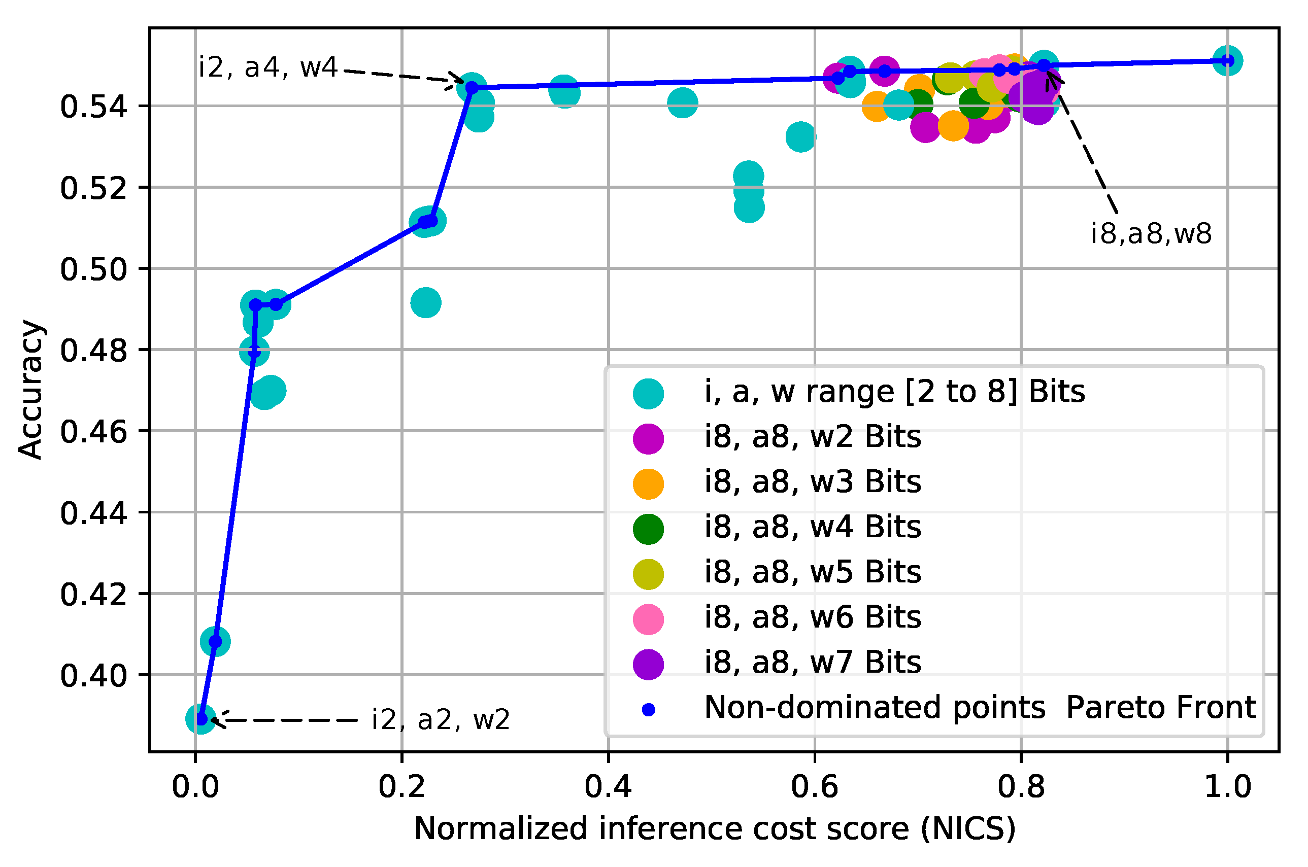
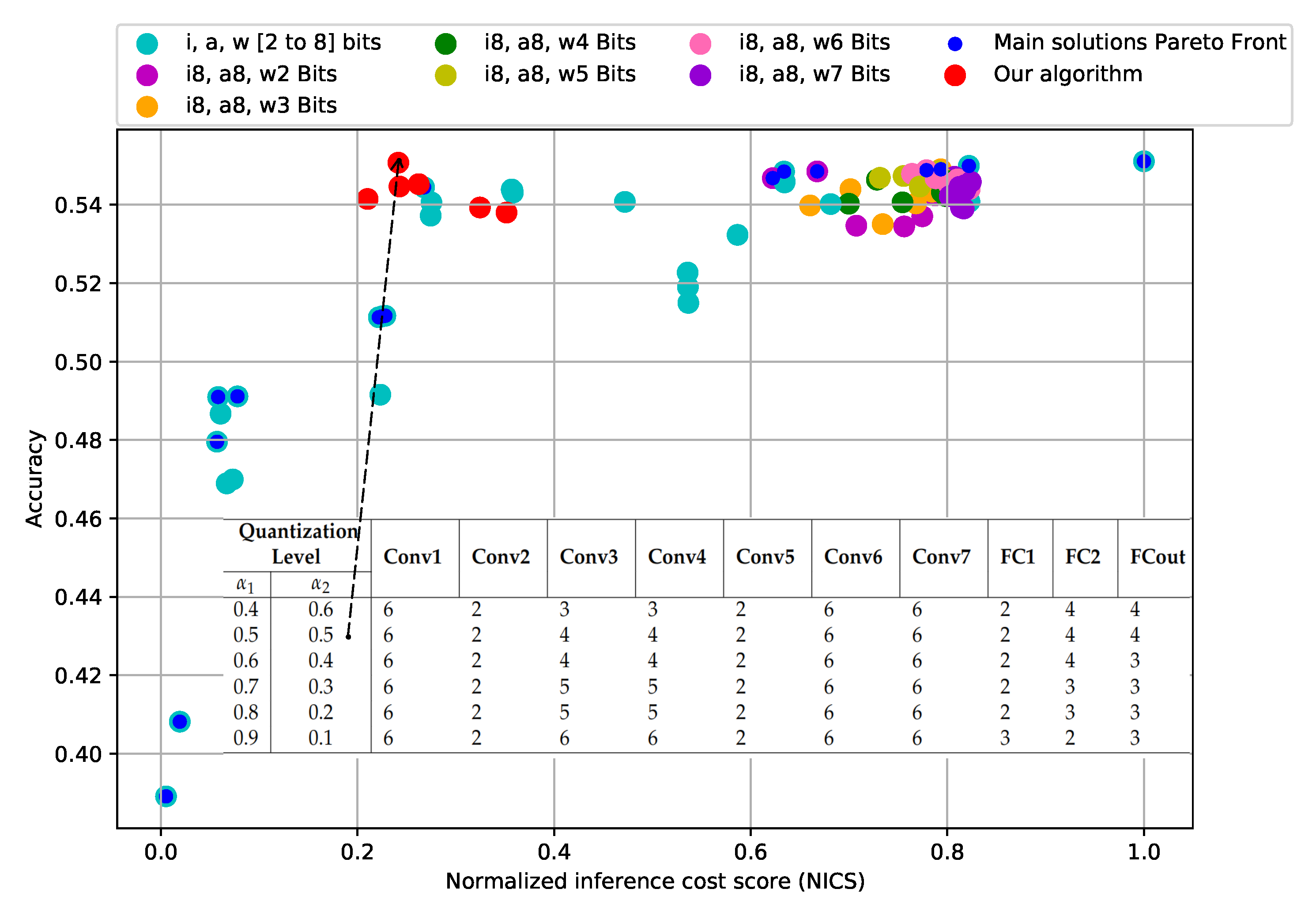
Figure 4 shows the solutions represented by their degree of quantization in aquamarine color. Notice that we intentionally do not discriminate between the quantization levels. Following this figure, it is possible to select one of the quantization options quickly; the choice will depend on how much accuracy we are willing to sacrifice in search of a lower inference cost. In this case, performing a Pareto optimal analysis can identify the quantizations with the best solutions so far. For example, the configuration ($i2,a2,w2$), the one located at the bottom-left corner in which all layers (input, activations, and weights) are quantized at 2 bits, shows the lowest inference cost equivalent to a 99.4% reduction. Nevertheless, this solution also offers the lowest classification accuracy with a drop in accuracy to 29.3%. On the contrary, the benchmark quantization ($i8,a8,w8$), in the upper right corner, shows the highest accuracy, which is similar to that of the unquantized model, but with a higher inference cost. However, it is possible to find a middle ground that allows for a sound inference cost reduction and acceptable accuracy.

For instance, when applying the configuration ($i2,a4,w4$), the accuracy drop is only about 1.2% regarding the highest. Moreover, the inference cost is reduced by 73.2%. Besides the good results regarding the quantization objective (i.e., good accuracy at lower inference cost), this last configuration also shows us that each quantized parameter (input, activations, and weights) has an independent effect on the accuracy and the inference cost. Therefore, we can analyze the impact of each layer in the second stage of the process.

Using the results, we compute Spearman’s correlation coefficient to identify the parameter that most influences the trade-off.

Table 2. Degree of correlation between the quantified parameters (input, activations, weights) and the total BOPS, accuracy, and NICS. The weight is the parameter with the highest correlation.

	Total BOPS	NICS	Accuracy
Input	0.351	0.295	0.275
Activations	0.470	0.336	0.442
Weights	0.893	0.955	0.790

shows the dependency between quantized parameters and their effects on NICS and accuracy. Quantizing the input, which corresponds to the I/Q signal used to train the model, does not significantly affect accuracy. For instance, the correlation coefficient has values of 0.295 and 0.275, corresponding to NICS and accuracy, respectively, representing low dependency, where the highest correlation coefficient is one. Regarding activations, the correlation shows that they have a mid-strong relationship with accuracy, higher than NICS. This means that quantizing the activations impacts the accuracy (e.g., does not heavily reduce the accuracy) but barely affects the inference cost. On the contrary, quantizing the weights correlates strongly with NICS and, to a lesser extent, with accuracy. With a correlation of 0.955, it is clear that the parameters that, when quantified, have the most significant impact in reducing inference cost are the weights. Moreover, it can also be seen that the accuracy is barely affected, having a value of 0.790, which is considered to be high. This indicates that we can quantize the weights to obtain similar accuracy at a reduced inference cost regarding the reference model.

5.2. Stage 2: Layered Evaluation, Analyzing the Impact of Quantization per Layer

In this experiment, we independently quantized the weights of each layer over a range of 2 to 8 bits. Contrary to the previous stage, we used the full range in quantization bits. The quantization of inputs, activations, and non-considered layers was set to 8 bits. This was due to the results observed in the previous section, where it was shown that quantifying these two parameters does not strongly affect the inference cost and classification accuracy. An example of how this stage was carried out is shown in

Table 3. Example of quantization in each layer independently; in this case, the inputs and activations were statically set to a given value (e.g., 8 bits) while the quantization values of the weights were varied in each run at a given layer (e.g., 2 bits).

VG10 1D CNN	Run
	1	2	3	4	5	6	7	8	9	10
Conv 1 (CNN L1)	2	8	8	8	8	8	8	8	8	8
Conv 2 (CNN L2)	8	2	8	8	8	8	8	8	8	8
Conv 3 (CNN L3)	8	8	2	8	8	8	8	8	8	8
Conv 4 (CNN L4)	8	8	8	2	8	8	8	8	8	8
Conv 5 (CNN L5)	8	8	8	8	2	8	8	8	8	8
Conv 6 (CNN L6)	8	8	8	8	8	2	8	8	8	8
Conv 7 (CNN L7)	8	8	8	8	8	8	2	8	8	8
FC 1 (D1)	8	8	8	8	8	8	8	2	8	8
FC 2 (D2)	8	8	8	8	8	8	8	8	2	8
FC out (D3)	8	8	8	8	8	8	8	8	8	2

, where a particular layer is quantized at 2 bits, keeping the remaining layers quantized at 8 bits. As can be inferred, for the VGG10 1D-CNN, we executed ten runs per quantization level.

5.3. Stage 3: Data Dispersion and Spearman Mapping, Distribution of the Results by Layer

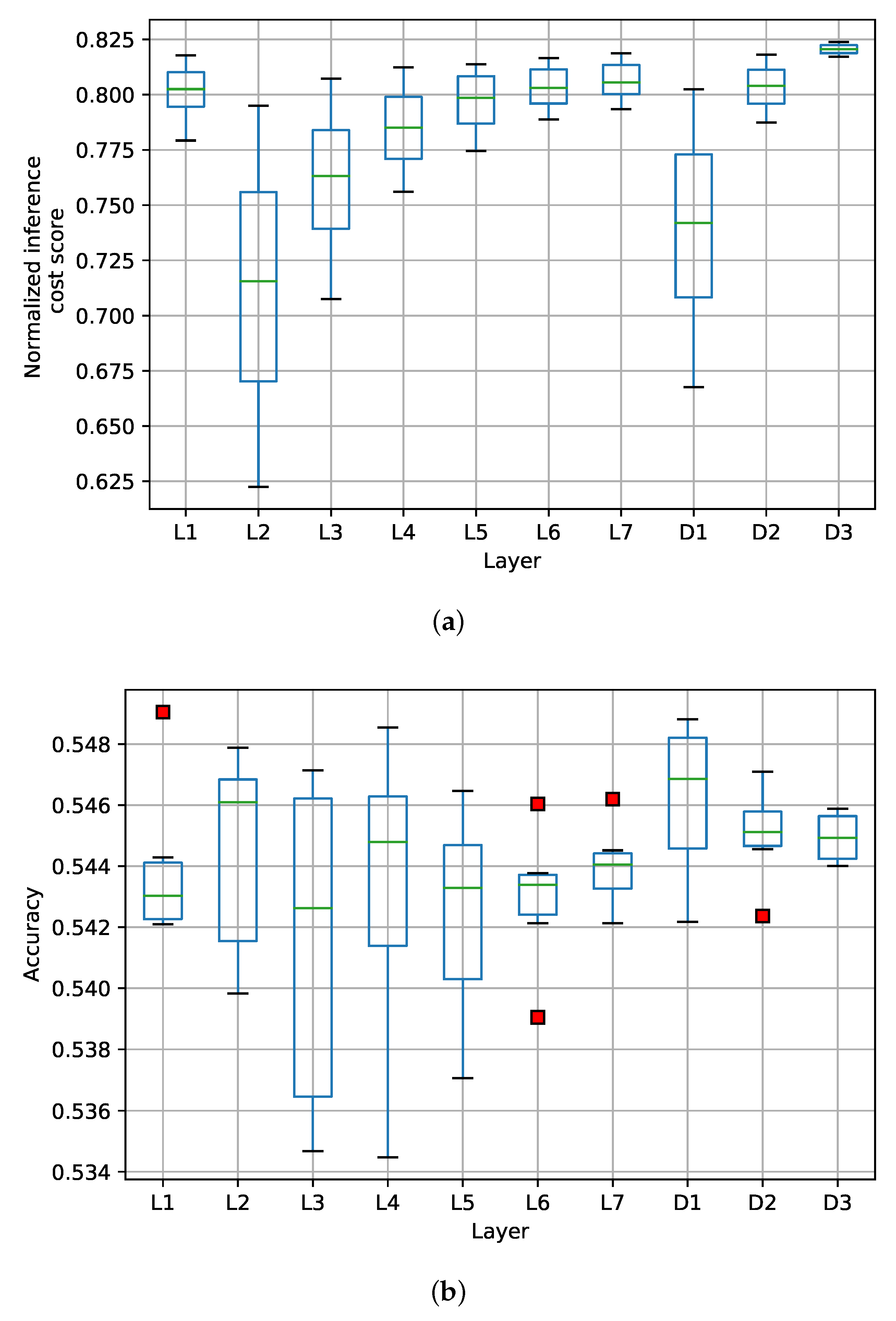
We obtained the accuracy and the inference cost for each configuration ($i8,a8,w$) in which the quantized value for the weights in a given layer were varied. Then, we analyzed the data distribution of those results, i.e., whether it was possible to define a specific behavior that would shed light on possible alternatives for quantification by layer discrimination. Figure 5a shows the box plot of the mean, median, and quartiles of the results obtained in the previous stage per layer and their impact on the inference cost. The figure shows that NICS is symmetric in the bit range used in the experiments. In this sense, it is observed that layer two (CNN L2) has the most significant impact on the reduction of the NICS, and to a lesser extent, layers three (CNN L3) and four (CNN L4). However, the input layer (CNN L1) does not significantly impact the computational cost reduction when quantified in the range of 2 to 8 bits. As for the FC layers, it is observed that the first dense layer (D1) significantly reduces the computational cost when quantized, but the output layer (D3) does not.

Furthermore, Figure 5a shows that each quantized layer has an exponential effect on the computational cost reduction; this behavior is due to the max pooling filter applied to the output of the convolutional layers. Similarly, Figure 5b shows the box plot of the results obtained and their impact on accuracy. From the figure, we can see that the quantization of each layer does not have a clear effect or general behavior regarding accuracy. This indicates that each layer could be quantized independently to achieve good accuracy with a lower computational cost. Nevertheless, we still need to determine the recommended quantization level for each model layer.

To determine the recommended quantization level per layer, we calculated the Spearman’s correlation coefficient with the results obtained from the previous stage. Figure 6 shows a box plot with Spearman’s correlation. As can be observed, it is possible to measure how strong the relationship is between each layer and the accuracy (see Figure 6a) and the inference cost (see Figure 6b) is. Concerning the accuracy, we observe that the results are dispersed. However, in most cases, the median of the data is above or below $\rho =0$, indicating a possible direction at the quantization level; that is, the quantization level should be increased ($\rho >0$) or decreased ($\rho <0$). In the case of the inference cost, we observe that there is no dispersion in the results. Only layers one, six, and fully connected layer two showed minimal dispersion. However, a similar approach can be followed to define the direction at the quantization level.

5.4. Stage 4: Selection of the Quantization Level per Layer

In the last stage of the methodology, we propose using the Spearman’s correlation coefficient as an indicator for the degree and direction of the relationship of each layer regarding the accuracy and inference cost. Then, since the Spearman’s correlation ranges from 1 to −1, we map the bit quantization levels from 4 to −4 to have an equivalent scale. This way, the highest possible quantization level (8 bits) is never exceeded. Since there are two variables we want to control (accuracy and inference cost), we applied Equation (7) to each of them. As a result, Equations (8) and (9) show how we define the scale to map the quantization bits according to the sign of the ratio. Using these equations, it is possible to determine a configuration that achieves the best compromise between accuracy and cost of inference. In the Equations, ${\beta }_{layer}$ is the bit selection from the accuracy perspective, while ${\delta }_{layer}$ is the bit selection from the inference cost perspective. $S_{a{M}_l}$ and $S_{n{M}_l}$ are the medians of the Spearman coefficient for a given layer, regarding accuracy and inference cost, respectively (see Figure 6).

$${\beta }_{layer}=\left\{\begin{array}{cc}4+\frac{\left(4\ast S_{a{M}_l}\right)+4}{2}\hfill & \mathrm{if}\rho ⩾1-\frac{6{\sum }_{i=1}^{n}Accurac{y}_i^2}{n\left(n^2-1\right)}\hfill \\ -4+\frac{\left(4\ast S_{a{M}_l}\right)+4}{2}\hfill & \mathrm{Otherwise}\hfill \end{array}\right.$$

(8)

$${\delta }_{layer}=\left\{\begin{array}{cc}-4+\frac{\left(4\ast S_{n{M}_l}\right)+4}{2}\hfill & \mathrm{if}\rho ⩾1-\frac{6{\sum }_{i=1}^{n}NIC{S}_i^2}{n\left(n^2-1\right)}\hfill \\ 4+\frac{\left(4\ast S_{n{M}_l}\right)+4}{2}\hfill & \mathrm{Otherwise}\hfill \end{array}\right.$$

(9)

Then, we can select a layer-discriminated quantization level for the model using Equation (10), which is a weighted sum that takes into account the contribution of each variable of interest. Q is the quantization level to be applied to a given layer, while ${\alpha }_1$ and ${\alpha }_2$ represent the importance given to accuracy or inference cost, with ${\alpha }_1+{\alpha }_2=1$. The result is a quantization level that considers both accuracy and inference cost.

$$Q=⌊{\alpha }_1\ast {\beta }_{layer}+{\alpha }_2\ast {\delta }_{layer}⌉$$

(10)

Finally, complementing the analysis methodology with Equations (8)–(10), we select the quantization levels discriminated on each layer in the DNN. Algorithm 3 shows the procedure’s pseudocode to perform stages three and four. We call this the LDQ algorithm. In LDQ, we define the necessary steps to determine the degree of quantization of each layer of a DNN for AMR. Note that the first part of the algorithm obtains the resulting accuracy and NICS metrics from the quantized models when varying the quantized values on each layer in Algorithm 2. Between lines 4 and 7, the solutions are mapped, grouping them by layers, and then analyzed with Spearman’s correlation (lines 8 and 9). In lines 10 and 11, using Equations (8) and (9), the decision threshold for each layer of the DNN is obtained. Finally, the quantification values are obtained between lines 13 and 17. Note that in this part, the alpha parameters allow different quantification configurations to be obtained depending on the importance assigned to them following Equation (10).

Algorithm 3 Stage 3 and 4: Layered Discriminated Quantization LDQ.

Require: Set E from Algorithm 2

Require: Set L with the layers of M to be quantized

Require:${\alpha }_1\in range[0,1]$ and ${\alpha }_2\in range[0,1]$, where ${\alpha }_1+{\alpha }_2=1$

1: for $l\in \left|L\right|$ do

2:    $E_n\leftarrow \left[\right]$

3:    $E_a\leftarrow \left[\right]$

4:    for $w\in W$ do

5:     $E_n=E_n\cap E\{l,w\}\left[0\right]$

6:     $E_a=E_1\cap E\{l,w\}\left[1\right]$

7:    end for

8:    $S_{a{M}_l}\leftarrow$ Calculate Spearman’s correlation analysis on $E_a$

9:    $S_{n{M}_l}\leftarrow$ Calculate Spearman’s correlation analysis on $E_n$

10:   ${\beta }_{laye{r}_l}=$ Apply Equation (8) using $S_{a{M}_l}$

11:   ${\delta }_{laye{r}_l}=$ Apply Equation (9) using $S_{n{M}_l}$

12: end for

13: for $j;j++;|{\alpha }_1|$ do

14:    for $l\in \left|L\right|$ do

15:     $Q\{{\alpha }_1\left[j\right],{\alpha }_2\left[j\right]\}\left[l\right]\leftarrow$ Apply Equation (10) with parameters ${\alpha }_1={\alpha }_1\left[j\right]$

16: ${\beta }_{layer}={\beta }_{laye{r}_l}$, ${\alpha }_2={\alpha }_2\left[j\right]$, and ${\delta }_{layer}={\delta }_{laye{r}_l}$

17:    end for

18: end for

19: Return E

5.5. Classification Evaluation

This section evaluates the configurations obtained from the layer discrimination analysis. This exercise aims to determine a suitable model configuration with a low bit size but that simultaneously does not compromise accuracy. Figure 7 shows, in red, the configurations obtained following the methodology described in the previous section. The solutions obtained with the quantizations used in the screening stage are also shown. The figure shows the two best results when the CNN model is quantized following the configuration $c1=\left[6,2,3,3,2,6,6,2,4,4\right]$ and $c2=\left[6,2,4,4,2,6,6,2,4,4\right]$. Configuration $c1$ has an accuracy of 0.541 and an inference cost of 0.210, while configuration $c2$ has an accuracy of 0.550 and an inference cost of 0.241, equivalent to 78.9% and 75.8% lower computational inference cost with respect to the non-quantized model. However, the reduction in accuracy is only 1.74% in the former case and 0.06% in the latter compared to the reference model. Therefore, we have shown that by independently quantizing every layer of the model, we can achieve similar performance to the reference model but at much lower computational cost.

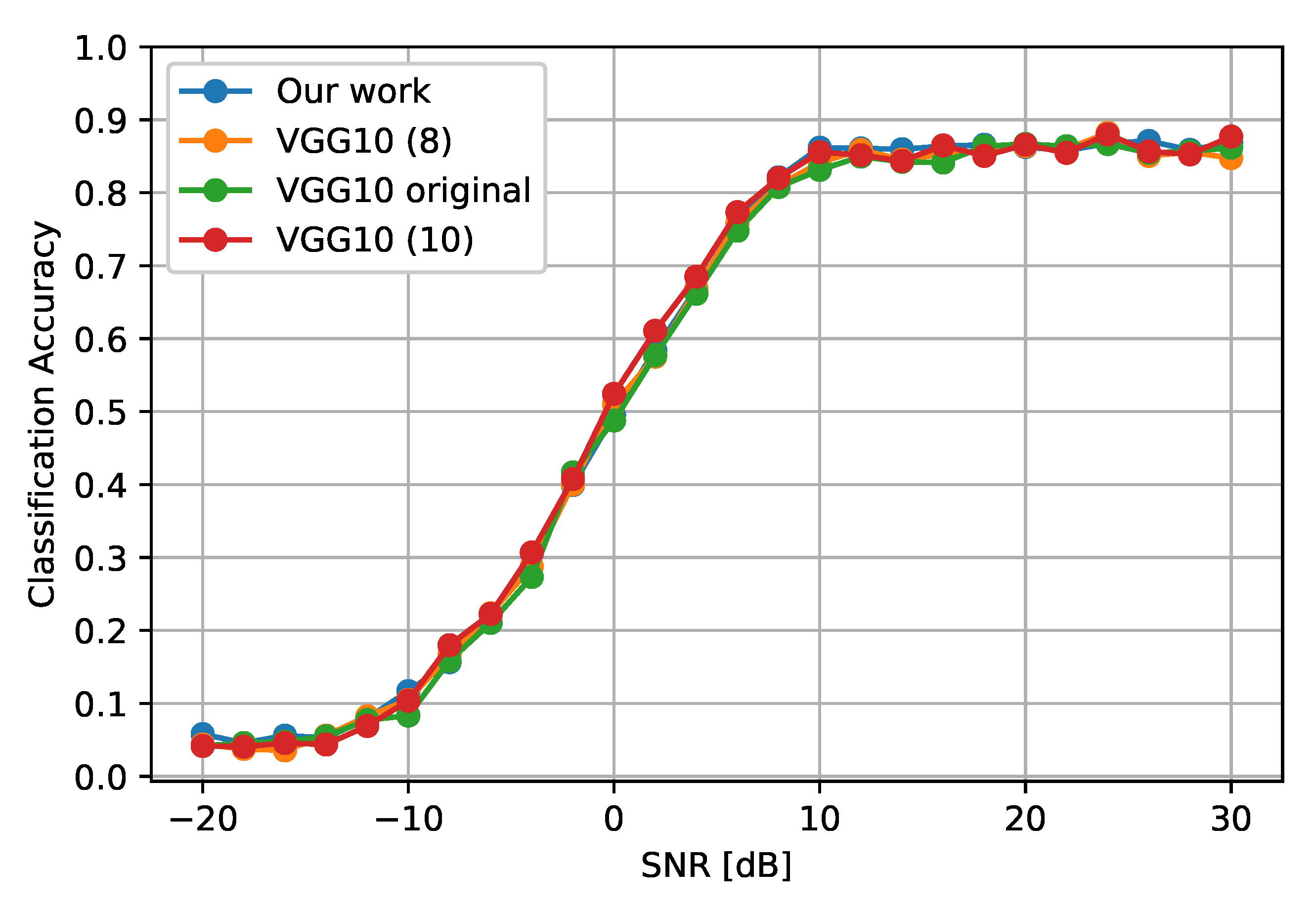
To verify this result, we compare the modulation classification accuracy of a configuration given by the methodology against the 8- and 10-bit quantized reference model. Since 8-bit quantization values were used as the basis for experimental quantization, we defined a reference model whose values were above any other test settings and could be used as a benchmark. Figure 8 shows the accuracy of the original model (not quantized), the 8- and 10-bit quantized model, and configuration $c2$. 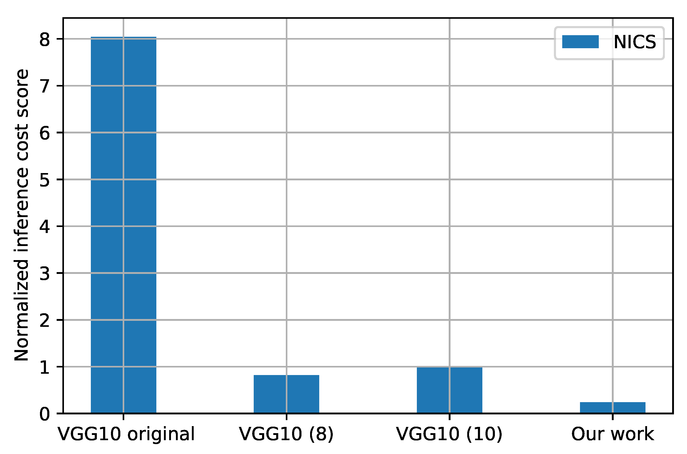Notice that all the layers are quantized at 8 and 10 bits in their respective versions. As we can see, the accuracy of all models is similar across different SNR values. As expected, the inference cost in Figure 9 is much lower in the quantized models than in the original model. In addition, a significant difference is observed in the solution found by using the methodology proposed in this paper.

6. Conclusions and Future Work

New-generation communications are geared toward coverage, service quality, and greater bandwidth with better use of available resources. In this sense, AI and parallel processing are tools that are called to support this type of task in modern radio systems. However, implementing DL algorithms in hardware is a non-trivial task due to the reduced ability to support large models. This has created a gap between research on intelligent communication algorithms and the implementation of such algorithms in radios. To close this gap, quantization is a technique that reduces the computational cost (e.g., model size in memory, number of operations, among others) of DL models, so that they can be deployed in devices with limited computational resources such as FPGA.

However, most of the proposed quantization methods for DL models apply the same quantization level to all the trainable parameters in the model, including inputs, activations, and weights. On the contrary, this article proposes a methodology to analyze the impact on accuracy against the inference cost of a quantized DNN model. Then, depending on the quantization level, a similar accuracy to the non-quantized model can be achieved at a much-reduced inference cost. Furthermore, our findings show that it is convenient to quantize the layers independently, as each layer has a different effect on inference cost and accuracy. In this sense, we showed that by independently quantizing the model layers according to the level of compromise in the model’s performance, an accuracy close to that obtained with the same model without quantization could be obtained.

In future work, we want to use our methodology to find the appropriate quantization level using other DNN architectures for AMR. In addition, the combination of our method with other quantization techniques or in combination with pruning remains to be addressed, which could provide an even more significant reduction in the inference cost and validation to the generality of the proposed approach. We will also validate our methodology with other DL architectures solving the same problem and DL architectures used to solve other related problems at the radio receiver side that will benefit from obtaining low-computational-cost models. Finally, we will complement our experimental results with performance evaluations of some of the resulting models as a part of a wireless communication system running on an FPGA. This is fundamental to provide further quantitative results of the trade-off between model accuracy and other metrics related to the model size, such as energy consumption and processing speed.

References

1. Bkassiny, M.; Li, Y.; Jayaweera, S.K. A Survey on Machine-Learning Techniques in Cognitive Radios. IEEE Commun. Surv. Tutor. 2013, 15, 1136–1159. [Google Scholar] [CrossRef]
2. Garhwal, A.; Bhattacharya, P.P. A survey on dynamic spectrum access techniques for cognitive radio. arXiv 2012, arXiv:1201.1964. [Google Scholar] [CrossRef]
3. Zhu, Z.; Nandi, A.K. Automatic Modulation Classification: Principles, Algorithms and Applications; John Wiley & Sons: Hoboken, NJ, USA, 2014. [Google Scholar] [CrossRef]
4. Dobre, O.A. Signal identification for emerging intelligent radios: Classical problems and new challenges. IEEE Instrum. Meas. Mag. 2015, 18, 11–18. [Google Scholar] [CrossRef]
5. O’Shea, T.J.; Corgan, J.; Clancy, T.C. Convolutional Radio Modulation Recognition Networks. In Proceedings of the Engineering Applications of Neural Networks; Jayne, C., Iliadis, L., Eds.; Springer International Publishing: Berlin/Heidelberg, Germany, 2016; pp. 213–226. [Google Scholar]
6. Dobre, O.A.; Abdi, A.; Bar-Ness, Y.; Su, W. Survey of automatic modulation classification techniques: Classical approaches and new trends. IET Commun. 2007, 1, 137–156. [Google Scholar] [CrossRef] [Green Version]
7. Liu, X.; Yang, D.; Gamal, A.E. Deep neural network architectures for modulation classification. In Proceedings of the 2017 51st Asilomar Conference on Signals, Systems, and Computers, Pacific Grove, CA, USA, 29 October–1 November 2017; pp. 915–919. [Google Scholar] [CrossRef] [Green Version]
8. Peng, S.; Jiang, H.; Wang, H.; Alwageed, H.; Zhou, Y.; Sebdani, M.M.; Yao, Y.D. Modulation Classification Based on Signal Constellation Diagrams and Deep Learning. IEEE Trans. Neural Netw. Learn. Syst. 2019, 30, 718–727. [Google Scholar] [CrossRef]
9. Mao, Y.; Dong, Y.Y.; Sun, T.; Rao, X.; Dong, C.X. Attentive Siamese Networks for Automatic Modulation Classification Based on Multitiming Constellation Diagrams. IEEE Trans. Neural Netw. Learn. Syst. 2021, 1–15. [Google Scholar] [CrossRef]
10. Tilghman, P. Will rule the airwaves: A DARPA grand challenge seeks autonomous radios to manage the wireless spectrum. IEEE Spectr. 2019, 56, 28–33. [Google Scholar] [CrossRef]
11. Camelo, M.; Soto, P.; Latré, S. A General Approach for Traffic Classification in Wireless Networks using Deep Learning. IEEE Trans. Netw. Serv. Manag. 2021, 1. [Google Scholar] [CrossRef]
12. Garcia-Saavedra, A.; Costa-Pérez, X. O-RAN: Disrupting the Virtualized RAN Ecosystem. IEEE Commun. Stand. Mag. 2021, 1–8. [Google Scholar] [CrossRef]
13. Budgett, S.; de Waard, P. Quantized neural networks for modulation recognition. In Proceedings of the Artificial Intelligence and Machine Learning for Multi-Domain Operations Applications IV SPIE, Orlando, FL, USA, 3 April–13 June 2022; Volume 12113, pp. 397–412. [Google Scholar]
14. Blott, M.; Preußer, T.B.; Fraser, N.J.; Gambardella, G.; O’Brien, K.; Umuroglu, Y.; Leeser, M.; Vissers, K. FINN-R: An end-to-end deep-learning framework for fast exploration of quantized neural networks. ACM Trans. Reconfigurable Technol. Syst. (TRETS) 2018, 11, 1–23. [Google Scholar] [CrossRef]
15. Kumar, S.; Mahapatra, R.; Singh, A. Automatic Modulation Recognition: An FPGA Implementation. IEEE Commun. Lett. 2022, 26, 2062–2066. [Google Scholar] [CrossRef]
16. Kumar, N.; Rawat, M.; Rawat, K. Software-defined radio transceiver design using FPGA-based system-on-chip embedded platform with adaptive digital predistortion. IEEE Access 2020, 8, 214882–214893. [Google Scholar] [CrossRef]
17. Umuroglu, Y.; Fraser, N.J.; Gambardella, G.; Blott, M.; Leong, P.; Jahre, M.; Vissers, K. Finn: A framework for fast, scalable binarized neural network inference. In Proceedings of the 2017 ACM/SIGDA International Symposium on Field-Programmable Gate Arrays, Monterey, CA, USA, 22–24 February 2017; pp. 65–74. [Google Scholar]
18. Pappalardo, A.; Umuroglu, Y.; Blott, M.; Mitrevski, J.; Hawks, B.; Tran, N.; Loncar, V.; Summers, S.; Borras, H.; Muhizi, J.; et al. QONNX: Representing Arbitrary-Precision Quantized Neural Networks. arXiv 2022, arXiv:2206.07527. [Google Scholar]
19. Haggui, H.; Affes, S.; Bellili, F. FPGA-SDR integration and experimental validation of a joint DA ML SNR and doppler spread estimator for 5G cognitive transceivers. IEEE Access 2019, 7, 69464–69480. [Google Scholar] [CrossRef]
20. Reiter, P.; Karagiannakis, P.; Ireland, M.; Greenland, S.; Crockett, L. FPGA acceleration of a quantized neural network for remote-sensed cloud detection. In Proceedings of the 7th International Workshop on On-Board Payload Data Compression, Virtual, 21–23 September 2020. [Google Scholar]
21. Lin, Y.; Zhao, H.; Tu, Y.; Mao, S.; Dou, Z. Threats of adversarial attacks in DNN-based modulation recognition. In Proceedings of the IEEE INFOCOM 2020-IEEE Conference on Computer Communications, Toronto, ON, Canada, 6–9 July 2020; pp. 2469–2478. [Google Scholar]
22. Goodfellow, I.; Bengio, Y.; Courville, A. Deep Learning; MIT Press: Cambridge, MA, USA, 2016. [Google Scholar]
23. Kim, S.H.; Kim, J.W.; Doan, V.S.; Kim, D.S. Lightweight deep learning model for automatic modulation classification in cognitive radio networks. IEEE Access 2020, 8, 197532–197541. [Google Scholar] [CrossRef]
24. Hiremath, S.M.; Behura, S.; Kedia, S.; Deshmukh, S.; Patra, S.K. Deep learning-based modulation classification using time and stockwell domain channeling. In Proceedings of the 2019 National Conference on Communications (NCC), Bangalore, India, 20–23 February 2019; pp. 1–6. [Google Scholar]
25. Wang, Y.; Liu, M.; Yang, J.; Gui, G. Data-driven deep learning for automatic modulation recognition in cognitive radios. IEEE Trans. Veh. Technol. 2019, 68, 4074–4077. [Google Scholar] [CrossRef]
26. Qing Yang, G. Modulation classification based on extensible neural networks. Math. Probl. Eng. 2017, 2017, 6416019. [Google Scholar] [CrossRef] [Green Version]
27. Zhang, D.; Ding, W.; Zhang, B.; Xie, C.; Li, H.; Liu, C.; Han, J. Automatic modulation classification based on deep learning for unmanned aerial vehicles. Sensors 2018, 18, 924. [Google Scholar] [CrossRef]
28. Huang, S.; Dai, R.; Huang, J.; Yao, Y.; Gao, Y.; Ning, F.; Feng, Z. Automatic modulation classification using gated recurrent residual network. IEEE Internet Things J. 2020, 7, 7795–7807. [Google Scholar] [CrossRef]
29. Fu, X.; Gui, G.; Wang, Y.; Ohtsuki, T.; Adebisi, B.; Gacanin, H.; Adachi, F. Lightweight automatic modulation classification based on decentralized learning. IEEE Trans. Cogn. Commun. Netw. 2021, 8, 57–70. [Google Scholar] [CrossRef]
30. Zhang, X.; Zhao, H.; Zhu, H.; Adebisi, B.; Gui, G.; Gacanin, H.; Adachi, F. NAS-AMR: Neural Architecture Search Based Automatic Modulation Recognition for Integrated Sensing and Communication Systems. IEEE Trans. Cogn. Commun. Netw. 2022, 8, 1374–1386. [Google Scholar] [CrossRef]
31. Ali, A.; Yangyu, F.; Liu, S. Automatic modulation classification of digital modulation signals with stacked autoencoders. Digit. Signal Process. 2017, 71, 108–116. [Google Scholar] [CrossRef]
32. Liu, Y.; Liu, Y.; Yang, C. Modulation recognition with graph convolutional network. IEEE Wirel. Commun. Lett. 2020, 9, 624–627. [Google Scholar] [CrossRef]
33. Tu, Y.; Lin, Y. Deep neural network compression technique towards efficient digital signal modulation recognition in edge device. IEEE Access 2019, 7, 58113–58119. [Google Scholar] [CrossRef]
34. Gunst, R.F.; Mason, R.L. Fractional factorial design. Wiley Interdiscip. Rev. Comput. Stat. 2009, 1, 234–244. [Google Scholar] [CrossRef]
35. Ducasse, Q.; Cotret, P.; Lagadec, L.; Stewart, R. Benchmarking Quantized Neural Networks on FPGAs with FINN. In Proceedings of the DATE Friday Workshop on System-Level Design Methods for Deep Learning on Heterogeneous Architectures, Virtual, 5 February 2021. [Google Scholar]
36. Bacchus, P.; Stewart, R.; Komendantskaya, E. Accuracy, training time and hardware efficiency trade-offs for quantized neural networks on fpgas. In Proceedings of the International Symposium on Applied Reconfigurable Computing; Springer: Berlin/Heidelberg, Germany, 2020; pp. 121–135. [Google Scholar]
37. O’Shea, T.J.; Roy, T.; Clancy, T.C. Over-the-Air Deep Learning Based Radio Signal Classification. IEEE J. Sel. Top. Signal Process. 2018, 12, 168–179. [Google Scholar] [CrossRef]
38. Simonyan, K.; Zisserman, A. Very deep convolutional networks for large-scale image recognition. arXiv 2014, arXiv:1409.1556. [Google Scholar]
Figure 1. General scheme of an SDR device. Two general stages are identified, the first is the RF-front-end, and the second is the baseband processing stage. FPGA is the closest hardware accelerator to the RF-front-end; it is here where DL algorithms can be downloaded to fulfill specific CR tasks. Taken from [16].
Algorithms 15 00441 g001
Figure 2. Workflow from Brevitas to the FPGA.
Algorithms 15 00441 g002
Figure 3. Proposed methodology based on fractional factorial design.
Algorithms 15 00441 g003
Figure 4. Effect of quantization in the VGG10 1D-CNN architecture regarding the accuracy and inference cost. Inputs, activations, and weights are quantized in a range of 2 to 8 bits in the first stage (in aquamarine). Points in different colors represent the degree of quantization in the weights (see the second-stage methodology). In blue, the points with the best solutions obtained thus far with the Pareto front are highlighted.
Algorithms 15 00441 g004
Figure 5. Impact of quantization applied in the VGG10 1D-CNN architecture proposed by [37] used in the classification of communication signals. Panel (a) shows the effect of the reduction in computational cost observed in each CNN layer. Panel (b) shows the accuracy observed at each layer. In this case, the red dots indicate outlier accuracy values corresponding to configurations with a high degree of quantization.
Algorithms 15 00441 g005
Figure 6. Spearman’s correlation per layer. Panel (a) shows the accuracy and Panel (b) shows the NICS against each quantized CNN layer. Note that a correlation is negligible when ρ < | 0.1 | , low when | 0.1 | < ρ < = | 0.3 | , medium when | 0.3 | < ρ < = | 0.5 | , and strong or high when ρ > | 0.5 | .
Algorithms 15 00441 g006
Figure 7. Configurations obtained following the proposed methodology (in red). The solutions obtained in previous phases are also shown. Notice that by varying α 1 and α 2 , different configurations can be obtained that were not found in the initial experimentation analyzed with the Pareto optimum.
Algorithms 15 00441 g007
Figure 8. Modulation classification accuracy of the original (unquantized) model and the quantized versions with different SNR values.
Algorithms 15 00441 g008
Figure 9. Comparison of the quantized VGG10 1D-CNN model versus the non-quantized.
Algorithms 15 00441 g009