Vineyard Gap Detection by Convolutional Neural Networks Fed by Multi-Spectral Images

Abstract

This paper focuses on the gaps that occur inside plantations; these gaps, although not having anything growing in them, still happen to be watered. This action ends up wasting tons of liters of water every year, which translates into financial and environmental losses. To avoid these losses, we suggest early detection. To this end, we analyzed the different available neural networks available with multispectral images. This entailed training each regional and regression-based network five times with five different datasets. Networks based on two possible solutions were chosen: unmanned aerial vehicle (UAV) depletion or post-processing with external software. The results show that the best network for UAV depletion is the Tiny-YOLO (You Only Look Once) version 4-type network, and the best starting weights for Mask-RCNN were from the Tiny-YOLO network version. Although no mean average precision (mAP) of over 70% was achieved, the final trained networks managed to detect mostly gaps, including low-vegetation areas and very small gaps, which had a tendency to be overlooked during the labeling stage.

1. Introduction

The increasing threat of global warming significantly affects the agricultural industry. This can be considered crucial for obtaining a decent quality of life for humans and deals with significant challenges, although contributing little to the global gross domestic product (GDP) [1,2]. One of the challenges to be fixed or diminished by the current research is water waste in agriculture that arises when a place within a crop field fails to grow plants. These spots are still watered by some irrigation systems, which results in water being wasted, monetary losses, and more energy wasted in watering [3,4]. The current methods of identifying these gaps include manual labor, which is expensive and inefficient due to the limited number of personnel available, the size of the fields, and the amount of time it takes. This motivated the search for methods to analyze vast swaths of land and quickly identify those gaps. To that end, modern developments in the agricultural research field will be the subject of research and could be employed as solutions for this matter. Nowadays, conventional agriculture is transitioning to a more digital and automatic version of itself, usually known as precision agriculture (PA), characterized by its usage of sensors, robotics, networks, and other engineering schemes to achieve more significant productivity and reduce energy and time waste. The technological upgrade in agriculture also led to the usage of unmanned aerial vehicles (UAV) [5,6,7], convolutional neural networks (CNN), wireless sensor networks [8], and Internet of Things (IoT) [9] as solutions for stage identification and supervision of crop maturation, inefficient irrigation systems, and transitioning conventional agriculture to a more sustainable industry overall [10].

Considering the above discussion, the current work proposes a methodology based on artificial intelligence (AI) and computer vision, where images obtained by a UAV are used to detect gaps in crop fields. In addition, the current study determines which combination of CNN and multi-spectral index could offer a better solution to be deployed in an UAV-based framework. The developed methodology would then help farmers rapidly identify trouble areas and solve the issue by replanting or avoiding irrigation of the area. Image maps are generated and fed to a CNN—the state-of-the-art method for computer vision tasks such as classification. This allows better detection and classification than traditional methods, since those lack the adaptability to new image data, lighting, and size without reworking the original algorithm [11]. On the one hand, artificial intelligence and CNN have been successfully used in several scientific fields, such as fashion [12], localization [13,14,15], and digital health [16]. On the other hand, UAV and artificial intelligence in conjunction have also been successfully applied in PA for crop disease identification [17] or flower classification [18,19]. Nevertheless, and as far as the author’s knowledge goes, gap detection, namely, for vineyard crops, has not been considered in the scientific literature.

The CNN networks that are the focus here can be categorized as regression-based networks, which include all YOLO network versions [20], and regional-based networks, from which we considered here the Mask-RCNN [21], as an example. The YOLO networks work by splitting an image into a $S\times S$ grid, and for each cell, predicting confidence scores and bounding boxes, where S is the two-dimensional grid size in pixels. Region-based Mask-RCNN networks, which are adaptations of RCNN networks [22], can perform semantic segmentation and work by feeding different regions of the input image into the network. Although region-based networks are known to be more accurate, regression-based networks are usually quicker and can work in real time, unlike the former. Since the final network is supposed to be deployed in a drone, it would be advantageous, although not necessary, to be able to work in real-time, since that decreases the amount of time taken into detecting the plantation gap [20,23].

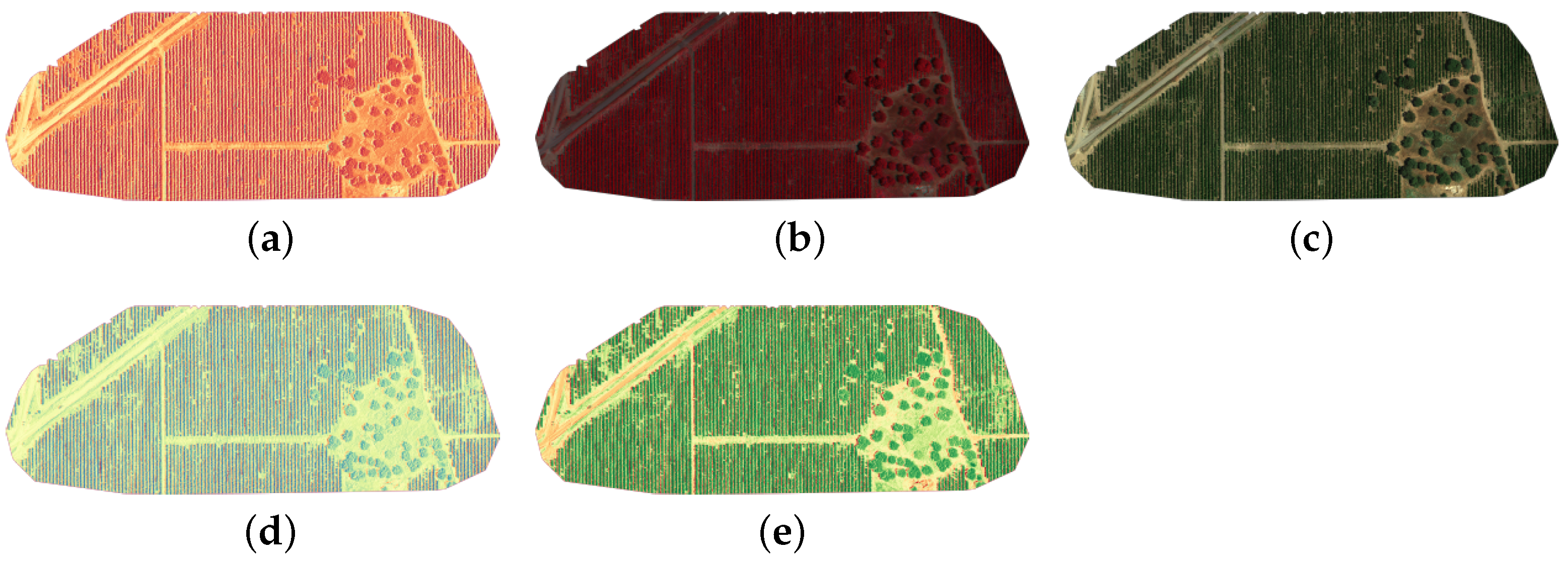
Besides considering which type of CNN network can be the best solution for detecting gaps, the data used in training said networks are also compared. The input images used included multi-spectral images and color image formats; these are listed below. Each one of these image types was generated through the mounted camera on the drone. The generated maps followed the aesthetic characteristics observed in Figure 1. These image maps represented entire fields spanning kilometers in length where each pixel was equivalent to 3 cm in the ground, and as mentioned previously, by looking in the original image maps, only the bigger gaps were easily identifiable by the researchers without zooming.

• NDWI is used for remote sensing of vegetation water from space. This type of supervision is used in agriculture and forest monitoring for fire risk evaluation, and is particularly suitable in the context of climate change. NDWI is responsive to changes in the water content of leaves in vegetation canopies and is less sensitive than NDVI to atmospheric changes [24]
• CIR uses the near-infrared (NIR) portion of the electromagnetic spectrum. This type of imagery is very useful when detecting different plant species, since the hue variations are more pronounced than in the visible light spectrum. CIR can also be used to detect changes in soil moisture [25].
• RGB is the most common image data available, being that it recreates images in the visible light spectrum. RGB is an additive color model where three colors—red, green, and blue—are combined to create a bigger color spectrum. From RGB, one can create GS images with image processing techniques, although, in this instance, several GS images were already provided, so it was chosen not to increase their number by converting the RGB images.
• NDRE combines NIR and a band between visible red and NIR. This index is very similar to NDVI but is more sensitive to different stages of crop maturation and is more suitable than NDVI for later crop seasons, after the vegetation has accumulated a bigger concentration of chlorophyll. This makes it so that NDRE is more fit for the entire cultivation season [26].
• NDVI is the oldest remote sensing technique used for vegetation monitoring. By observing different types of wavelengths (visible and non-visible light), one can determine the density of green vegetation in a patch of land. The pigment chlorophyll in plant leaves absorbs visible light (from 0.4 to 0.7 $\mathsf{\mu }$m) when doing photosynthesis, and the cell structure of the leaves reflects NIR. This index is better applied when trying to figure out how much plants cover a certain area, and can be great at detecting gaps in green crops [27].

The remainder of the paper is structured as follows. Section 2 summarizes previous related work. Section 3 provides an in-depth description of the different networks, the image dataset, the proposed method for the preprocessing stage, and the research methodology. Section 4 presents the obtained results, and Section 5 critically discusses those results. Finally, Section 6 concludes the work and discusses future research topics.

2. Related Works

Nowadays, the use of AI and UAVs in agriculture is well documented. UAVs are proposed as solutions for fertilizer and pesticide sprayers and crop supervision [28,29,30,31]. CNNs have been used for plant species classification, maturation stage identification, and disease detection in crops [17,18,32], and multi-spectral imaging has been used in conjunction with these tools as a way to improve classification and supervision tactics [33,34,35,36,37,38,39]. For this paper, the results were not tested in a drone. The focus was on determining which CNNs and with which image format this could be most easily achieved. Several networks were trained with datasets of different image formats or types for that goal.

This section outlines the different technologies that are or could be used to solve the problem presented in the introduction. When it comes to the field of computer vision, the histogram of gradient descent (HOG) is an algorithm that is good at distinguishing certain features in an image while ignoring the background image data; it is particularly good at identifying people and textual data [40]. To improve on this algorithm, researchers have been implementing machine learning techniques that can be used in a bigger array of data types and situations, which include the YOLO and RCNN networks.

As mentioned previously, although a real-time application is not necessary and the system can post-process the generated image from the UAV’s multispectral camera with exterior software, it would be advantageous to be able to detect the gaps in real-time, since it would significantly decrease the expense and time used in analyzing the data, but this adds a challenge, since UAV platforms do not usually have enough computing power and memory. The UAV would have to be able to generate the maps; input the images of the different multispectral types and formats into the network, which would need to be saved in memory; and return a complete map that points to the various places in the plantation where gaps were identified. Due to the sizes of the networks, it was decided to train YOLO and Tiny-YOLO versions of the original YOLO, YOLOv2, YOLOv3, and YOLOv4 networks; these are altered, more lightweight versions of the original YOLO networks. Custom versions of YOLO have been used in UAV research for real-time applications and proven to perform well as solutions [41,42,43]. Another network trained was Mask-RCNN, which, as mentioned previously, is not able to work in real-time, and therefore, is more appropriate in an external software, being that in this instance the UAV would not need to spend memory and computational power deploying the network. Mask-RCNN is one of the most common CNNs used in semantic segmentation, which allows identifying only the pixels that are part of the object which translates into a more precise localization of the plantation gap inside the generated map [20,21,22,23,44,45,46,47]. When it comes to the differences between all YOLO networks, it mainly comes down to increases in speed, accuracy, and precision from one version to the next. YOLOv3 was based around Darknet-53, a combination of Darknet-19, the basis of the YOLO and YOLOv2 architectures, and deep residual neural networks; and YOLOv4’s architecture is based around CSPDarknet-53.

Another relevant part of the solution is the use of a UAV instead of other supervision methods already in use in agriculture, for example, satellite imaging and Geographical Information Systems (GIS) [48,49,50,51]. Satellite data are easily accessible and already archived on the Internet and can image unlimited areas, which is advantageous in agriculture, although this is dependent on waiting for the satellite to pass near the right area. In addition, acquisition can easily be postponed if the weather conditions are not ideal. When it comes to GIS, the resolution is dependent on the size of the raster cell, which is inversely proportional to the resolution; this makes it so that one must find a balance between processing time and storage [52]. By using a UAV, visual information that has better resolution can be obtained, allowing the system to detect smaller gaps, during cloudy and non-cloudy days, at any time, without having to wait for the satellite to pass that region; and since the UAV is equipped with a multi-spectral camera, the maps can be generated instantly and later be processed.

This paper presents the results of training and testing Tiny-YOLO, YOLO, Tiny-YOLOv2, Tiny-YOLOv3, Tiny-YOLOv4, and Mask-RCNN with six different datasets: Normalized Difference Vegetation Index (NDVI), Normalized Difference Red-Edge (NDRE), Normalized Difference Water Index (NDWI), RGB (Red-Green-Blue), Gray-Scale (GS), and Color Infrared (CIR). When choosing the networks, it was important to take into account the limited computational power of UAVs. Regardless, this method was prioritized over other methods—for example, GIS and satellite imaging with cloud processing, because UAV allows the system to be used at any time, independently of weather conditions, unlike satellite imaging. The chosen networks all have the capability of being deployed in the final system due to being light in comparison with their full network counterparts.

3. Materials and Methods

We started by preprocessing the images, since the generated maps had a resolution of 3665 × 2539, which made it so that only the bigger gaps were easily identified. This is not ideal, since smaller gaps needed to be detected as well, and YOLO networks have difficulties with classifying smaller objects, as discussed in [20]. To improve detection, every map was cropped into smaller regions of 406 × 406, which made the creation of bounding boxes and polygons (in Mask-RCNN’s case) of the objects easier and helped the networks identify smaller gaps as a result. Cropping each map into several smaller images also increased the amount of data available for training and testing.

Firstly, only the regression-based networks were trained; this was decided so that the resulting weights could be reused as starting weights when training Mask-RCNN. Using pre-trained weights, also known as transfer learning [53,54], is a technique used when the knowledge gained from solving a certain problem is reused in a different but related problem. Since the regression-based networks were previously trained to identify rectangular regions encapsulating the gaps, these weights can be used to train Mask-RCNN, where the objective is to identify only the pixels related to the objects which would be inside these bounding boxes. The use of transfer learning with Mask-RCNN is common and shown to result in reliable systems that can correctly identify objects [55,56]. Mask-RCNN was fine-tuned to the dataset which only included training the region proposal network (RPN), the mask head layers, and the classifier layers, since the starting weights were already pre-trained. Fine-tuning is another technique of transfer learning where the network is not trained from the ground up and instead only the classification layers are re-trained with the new data; this is a technique applied to reduce the amount of training time [57,58]. Later in the research process, more maps were available, and since the results of the fine-tuning Mask-RCNN were not satisfactory, as will be discussed later, the new maps were processed and added to the datasets, and all layers of Mask-RCNN were retrained for a longer period. With this, all training procedures can be neatly divided into three distinct stages, listed below, where the parameters and methodology of each stage are described.

• Stage 1: Training all regression-based networks. For this, the networks in this repository [59] were trained with the following configurations: height and width of 406 pixels for input images, 32 batches, 4 subdivisions, 3 channels, momentum of 0.9, 0.0005 decay rate, 1.5 for saturation and exposure, a hue of 0.1, a learning rate of 0.001, and a maximum number of batches of 4000. The maximum number of batches determines how long the network will train for. The parameters of the network were not altered from the defaults found in the repository at any stage of training.
• Stage 2: Training ‘head’ layers of Mask-RCNN for 30 epochs. These layers included the region proposal network (RPN), the mask head layers, and the classifier layers. We used the Mask-RCNN network in this repository [60]. This network is based on feature pyramid network (FPN) and a ResNet101 as a backbone. The resulting weights of Stage 1 were fed as starting weights for Mask-RCNN. The configurations were not changed from the default ones in the repository configuration files.
• Stage 3: Continuation of Mask-RCNN training, but this time with ‘all’ layers being trained for 50 epochs. The same repository of Stage 2 was used once again, with the same configurations. The resulting weights of Stage 2 were used as starting weights for this stage.

The camera used to photograph the different crop fields was a MicaSense RedEdge-MX™. This camera has a resolution of 1280 × 960, a sensor size of 4.8 mm × 3.6 mm, a focal length of 5.4 mm, and a field of view of 47.2 degrees horizontally and 35.4 degrees vertically [61]. This camera was mounted onto the UAV and records five different multi-spectral band channels [31,62,63].

Although all regression-based networks can be applied to analyze and detect objects, in this situation, the objective was to deploy the best solution into a UAV, which does not flaunt a huge amount of memory [31]. Therefore, according to what was possible to train with the provided hardware, the tiny versions of the different YOLO networks, and YOLO (see Appendix A), were trained once for every training dataset.

The hardware used for training the networks presented in Table 3 was a computer with a processor Intel^® Core™ i7-9750H CPU @ 2.60 GHz × 12 and a NVIDIA GeForce GTX 1660 Ti/PCIe/SSE2 graphics card, and the languages and frameworks used were Python, Tensorflow, Keras, and OpenCV.

In this section, there are two subsections: images and datasets, and code and repositories. The images and datasets section is where we explain the differences between all image format types used in this research and the amounts of data in our datasets, and the code and repositories section presents the explanations of all code developed and repositories used to complete this paper’s research.

3.1. The Images and Datasets

Before training and testing, a dataset was created for each image format mentioned (see Figure 1). The generated maps were divided by file types, and one class object was identified in every image—the vine gap. The manual identification was made by one person. The software used to manually draw the bounding boxes is mentioned in the next section.

Images were prepared before training the CNN; this included cropping each map into same-sized pieces, that could or could not be overlapped with one another. Cropping the map into smaller images resulted in a closer look into a certain space of the field. By using zoomed images of fixed spaces, the neural networks can more easily detect the gaps in an image. This allows YOLO [20], and its successors, to work better, since YOLO networks give worse results when objects are farther away.

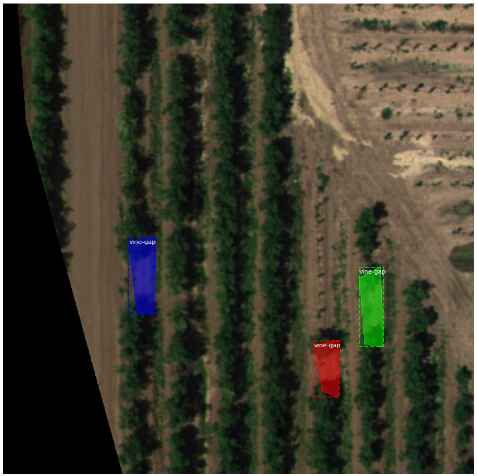
In Figure 2, the bounding boxes and labeled regions include parts of the top and bottom vegetation, which trained the networks to search for gaps encapsulated by plants. Although this is a better way to identify objects and regions, as it will be discussed, networks struggled with patches of dirt that mimicked these characteristics. As mentioned before, later in the research process, more generated maps were received, which were integrated into the datasets and increased the amount of data available to retrain Mask-RCNN. In

Table 1. Number of images per multi-spectral index. First dataset used for training. Total: total number of images; Train: total number of images used in training; Test: total number of images used for testing. Approximately 10% of Total was used for testing.

Multi-Spectral Index	Total	Train	Perc. (%) Train	Test	Perc. (%) Test
RGB	1696	1590	94%	106	6%
CIR	1575	1414	90%	161	10%
NDWI	1575	1418	90%	157	10%
NDRE	1352	1226	91%	126	9%
NDVI	327	281	86%	41	14%
GS	650	583	90%	67	10%

, we describe the number of images we had, after cropping each map, for each image type, and how much data we used in training and testing. We implemented a cropping algorithm (see Algorithm 1) that in conjunction with Algorithm 2 automatically divided each set into two subsets (training and testing) by giving a percentage of approximately how many images we wanted for testing. As shown in Table 1, we used 10% first, and later, when we received more images, we increased the testing data to approximately 20% due to having more images. As seen in Table 1 and

Table 2. Number of images per multi-spectral Index. Second dataset used for training. Total: total number of images; Train: total number of images used in training; Test: total number of images used for testing. Approximately 20% of Total was used for testing.

Multi-Spectral Index	Total	Train	Perc. (%) Train	Test	Perc. (%) Test
RGB	2429	1906	78%	523	22%
CIR	2018	1586	79%	432	21%
NDWI	2018	1615	80%	403	20%
NDRE	1795	1397	78%	398	22%
NDVI	665	554	83%	111	17%
GS	650	505	78%	145	22%

, the percentage amounts were not fixed; instead, they averaged out to the percentages discussed previously of 90–10% and 80–20%; this is because, as it was studied, there were no advantages in achieving perfect ratios in this case, and its effects would have been small, since it would have changed the datasets by a couple of images.

Algorithm 1 Crop images with overlap.

Find every X and Y that defines the borders of the new images for every $y_{value}$ in Y do    for every $x_{value}$ in X do      Split the image according to the coordinates      if Cropped image only contains $alpha$ values then         Skip Image      end if      Save cropped image as a new image    end for end for

Algorithm 2 Separate images into train batch and test batch.

Create a parent folder with each image format separated into different folders Percentage = fraction of images going into the test batch for every folder in directory do    for every file in folder do      Choose a random number in an interval      if number < percentage then         Move image to test batch folder      else         Move image to train batch folder      end if    end for end for

3.2. The Code and Repositories

Starting with the datasets, there were two steps: cropping each map into smaller, more manageable sections of about $406\times 406$ pixels, separating them into their respective training and testing datasets. At no point was the resolution of the input images changed when training the networks. When it came to the order of tasks, firstly Algorithm 1 was used to crop, with an overlap of 25%, and then Algorithm 2 organized them into training and test datasets.

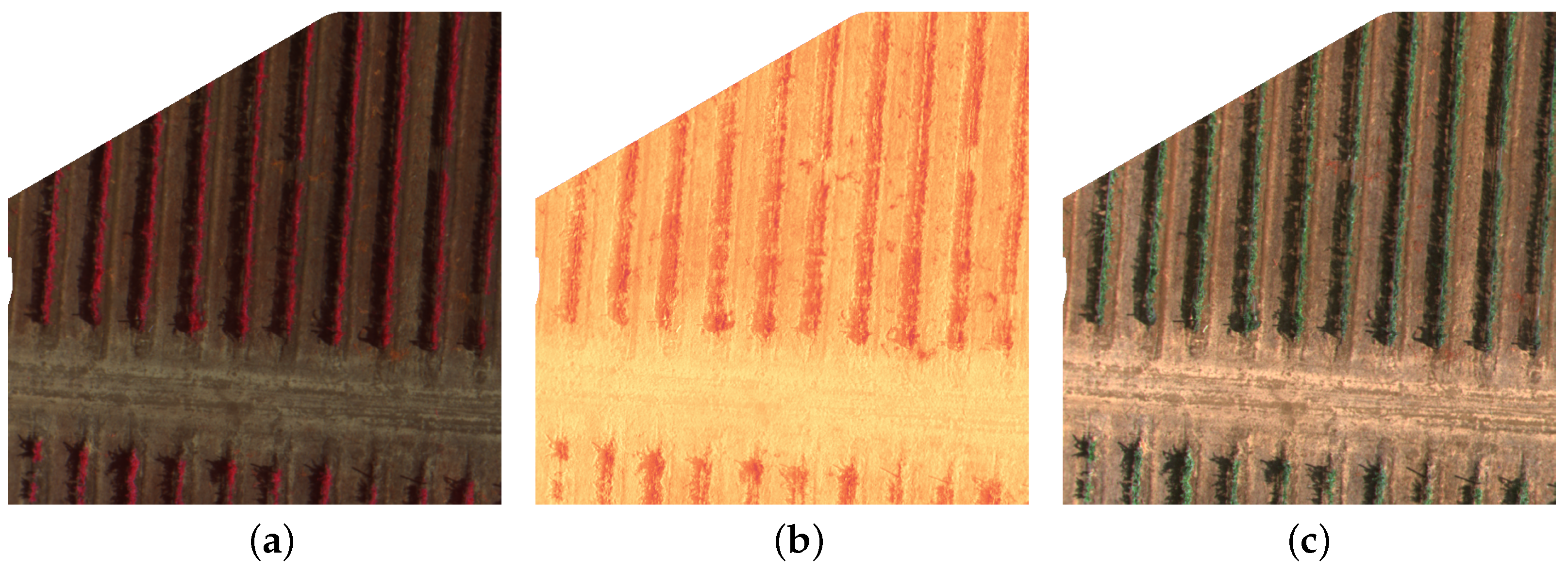
Algorithm 1 was developed to crop each map into the same number of cropped images; these images were then saved into their respective folders that identified their multi-spectral properties or image formats and saved under the same name when they were of the same region in similar maps, as represented in Figure 3. By giving the images in Figure 3 the same name, the bounding boxes only needed to be identified once, and generalized to the other same-named images on other datasets, which considerably reduced the preparation time.

Algorithm 2 was created to split each original dataset into two smaller collections of images, one for training and another for testing. When it came to the first datasets (see Table 1), a value of 0.1 was used for the percentage variable, and for the final datasets (see Table 2) the percentage value was 0.2. This explains why the train and test batches were not neatly divided into 90% and 10%, or 80% and 20%,, since the algorithm decided, based on the random chance, if an image was going to the train set or test set, but as can be observed in Table 1 and Table 2, each set, on average, was approximately 10% or 20% test data, as appropriate.

The true bounding boxes were defined using the repository YOLO-MARK from [64], and for the polygon regions for Mask-RCNN training, VGG Image Annotator [65] was used, for both training and testing datasets. These annotators require the presence of a researcher to manually delimit each rectangular ground truth box and polygon vertex. This method is very time expensive, but each vertex coordinate is saved in a file to later be fed into the network during the training stage.

It should be noticed that not every gap was caught and marked for training. These unmarked gaps that can be easily detected by human eyes were not chosen because it was determined that since these ’gaps’ had some minimal amount of vegetation, this could create uncertainty in the network; therefore, the gaps chosen were to be as empty of vegetation as possible, with top and bottom edges very defined. This does not exclude the human error that certainly arose during the manual delimitation of ground truth boxes.

Additionally, due to generating the maps at different times of day, the dataset is filled with images that, although they are from the same multi-spectral index, they are visibly dissimilar, which diversified each dataset. Further, some maps are diagonal or have slight angles, and some seem to have a more zoomed in picture of the field. With these slight variations, the chances of overfitting are smaller, and the resulting weights can be generalized more easily to different fields and times of the day.

4. Results

To evaluate and assess the quality of the different methods, standard performance metrics for object detection or instance segmentation were employed [66]. To that end, the $A{P}_{50}$ values for each pair of network and dataset were compared; those happen to be the bigger numbers, and $A{P}_{75}$ resulted in very small percentages; this is due to the way $A{P}_{50}$ and $A{P}_{75}$ are calculated, being that $A{P}_{50}$ counts as true a detection whose predicted bounding box overlaps 50% of the truth bounding box, which is equivalent to having an intersection over union (IoU) of 0.5, whereas $A{P}_{75}$ needs an overlap of 75% (IoU of 0.75), which were the settings used for

Table 3. Regression based networks training. $A{P}_{50}$: average precision with IoU of 0.5; $A{P}_{75}$: average precision with IoU of 0.75; Train: dataset used in training; Method: Network used for training.

Method	Train	${\mathbf{AP}}_{50}$	${\mathbf{AP}}_{75}$
YOLO	RGB	41.61%	2.07%
Tiny-YOLO	RGB	26.52%	0.30%
Tiny-YOLOv2	RGB	38.67%	6.65%
Tiny-YOLOv3	RGB	56.73%	11.82%
Tiny-YOLOv4	RGB	61.47%	19.62
YOLO	CIR	31.72%	2.79%
Tiny-YOLO	CIR	21.93%	0.49%
Tiny-YOLOv2	CIR	28.58%	1.16%
Tiny-YOLOv3	CIR	49.82%	4.92%
Tiny-YOLOv4	CIR	52.87%	12.39%
YOLO	NDRE	11.10%	1.34%
Tiny-YOLO	NDRE	4.37%	0.01%
Tiny-YOLOv2	NDRE	16.65%	0.76%
Tiny-YOLOv3	NDRE	46.20%	6.57%
Tiny-YOLOv4	NDRE	50.86%	11.96%
YOLO	NDWI	4.42%	0.00%
Tiny-YOLO	NDWI	0.67%	0.00%
Tiny-YOLOv2	NDWI	17.16%	0.57%
Tiny-YOLOv3	NDWI	42.97%	3.23%
Tiny-YOLOv4	NDWI	46.34%	4.09%
YOLO	GS	20.09%	0.30%
Tiny-YOLO	GS	11.99%	0.44%
Tiny-YOLOv2	GS	14.51%	1.89%
Tiny-YOLOv3	GS	29.61%	8.55%
Tiny-YOLOv4	GS	32.28%	10.04%
YOLO	NDVI	21.63%	3.33%
Tiny-YOLO	NDVI	18.61%	0.26%
Tiny-YOLOv2	NDVI	18.13%	0.11%
Tiny-YOLOv3	NDVI	27.79%	3.00%
Tiny-YOLOv4	NDVI	21.25%	6.11%

and

Table 4. Mask-RCNN ‘heads’ layers training for 30 epochs. Method: weights used + Mask-RCNN; Train: dataset used in training; $A{P}_{50}$: average precision with an IoU of 0.5; $A{P}_{75}$: average precision with an IoU 0.75.

Method	Train	${\mathbf{AP}}_{50}$	${\mathbf{AP}}_{75}$
YOLO + Mask-RCNN	RGB	21.42%	1.52%
Tiny-YOLO + Mask-RCNN	RGB	36.30%	4.03%
Tiny-YOLOv2 + Mask-RCNN	RGB	33.72%	2.17%
Tiny-YOLOv3 + Mask-RCNN	RGB	31.71%	3.78%
Tiny-YOLOv4 + Mask-RCNN	RGB	7.12%	0.12%
YOLO + Mask-RCNN	CIR	24.48%	1.66%
Tiny-YOLO + Mask-RCNN	CIR	36.67%	3.34%
Tiny-YOLOv2 + Mask-RCNN	CIR	23.96%	0.93%
Tiny-YOLOv3 + Mask-RCNN	CIR	36.02%	4.50%
Tiny-YOLOv4 + Mask-RCNN	CIR	19.30%	1.16%
YOLO + Mask-RCNN	NDRE	4.55%	0.47%
Tiny-YOLO + Mask-RCNN	NDRE	0.11%	0.0%
Tiny-YOLOv2 + Mask-RCNN	NDRE	0.02%	0.0%
Tiny-YOLOv3 + Mask-RCNN	NDRE	5.68%	1.94%
Tiny-YOLOv4 + Mask-RCNN	NDRE	0.0%	0.0%
YOLO + Mask-RCNN	NDWI	2.22%	0.0%
Tiny-YOLO + Mask-RCNN	NDWI	1.68%	0.0%
Tiny-YOLOv2 + Mask-RCNN	NDWI	11.69%	0.61%
Tiny-YOLOv3 + Mask-RCNN	NDWI	9.14%	0.0%
Tiny-YOLOv4 + Mask-RCNN	NDWI	1.20%	0.0%
YOLO + Mask-RCNN	NDVI	45.65%	6.88%
Tiny-YOLO + Mask-RCNN	NDVI	23.41%	1.61%
Tiny-YOLOv2 + Mask-RCNN	NDVI	37.95%	6.76%
Tiny-YOLOv3 + Mask-RCNN	NDVI	0.07%	0.0%
Tiny-YOLOv4 + Mask-RCNN	NDVI	9.87%	0.0%
YOLO + Mask-RCNN	GS	35.32%	6.46%
Tiny-YOLO + Mask-RCNN	GS	23.32%	1.75%
Tiny-YOLOv2 + Mask-RCNN	GS	18.91%	3.20%
Tiny-YOLOv3 + Mask-RCNN	GS	46.48%	6.48%
Tiny-YOLOv4 + Mask-RCNN	GS	15.38%	0.04%

. Therefore, if the ratio between the truth and predicted bounding boxes were to be diminished to 10%, the overall average precision would increase, which is demonstrated in

Table 5. Mask-RCNN ‘all’ layers training for 50 epochs. Method: weights used + Mask-RCNN; Train: dataset used in training; $A{P}_{10}$: average precision with an IoU of 0.10; $A{P}_{50}$: average precision with an IoU of 0.5; $A{P}_{75}$: average precision with an IoU 0.75.

Method	Train	${\mathbf{AP}}_{10}$	${\mathbf{AP}}_{50}$	${\mathbf{AP}}_{75}$
YOLO + Mask-RCNN	RGB	66.12%	56.55%	9.64%
Tiny-YOLO + Mask-RCNN	RGB	67.98%	60.88%	12.81%
Tiny-YOLOv2 + Mask-RCNN	RGB	66.42%	59.10%	15.33%
Tiny-YOLOv3 + Mask-RCNN	RGB	63.25%	57.46%	11.50%
Tiny-YOLOv4 + Mask-RCNN	RGB	64.07%	57.69%	9.18%
YOLO + Mask-RCNN	CIR	65.37%	52.56%	12.38%
Tiny-YOLO + Mask-RCNN	CIR	59.92%	53.69%	13.90%
Tiny-YOLOv2 + Mask-RCNN	CIR	61.90%	52.74%	8.46%
Tiny-YOLOv3 + Mask-RCNN	CIR	62.83%	52.14%	11.01%
Tiny-YOLOv4 + Mask-RCNN	CIR	63.53%	52.88%	5.86%
YOLO + Mask-RCNN	NDRE	43.76%	24.16%	2.07%
Tiny-YOLO + Mask-RCNN	NDRE	42.67%	23.60%	2.02%
Tiny-YOLOv2 + Mask-RCNN	NDRE	44.77%	25.22%	3.27%
Tiny-YOLOv3 + Mask-RCNN	NDRE	35.89%	21.17%	0.16%
Tiny-YOLOv4 + Mask-RCNN	NDRE	42.17%	24.19%	1.17%
YOLO + Mask-RCNN	NDWI	56.24%	34.98%	2.98%
Tiny-YOLO + Mask-RCNN	NDWI	58.21%	40.93%	7.57%
Tiny-YOLOv2 + Mask-RCNN	NDWI	52.19%	40.43%	2.38%
Tiny-YOLOv3 + Mask-RCNN	NDWI	59.69%	50.98%	8.30%
Tiny-YOLOv4 + Mask-RCNN	NDWI	55.05%	43.10%	7.17%
YOLO + Mask-RCNN	NDVI	51.06%	40.49%	5.43%
Tiny-YOLO + Mask-RCNN	NDVI	55.12%	41.92%	5.39%
Tiny-YOLOv2 + Mask-RCNN	NDVI	58.69%	47.08%	3.91%
Tiny-YOLOv3 + Mask-RCNN	NDVI	57.50%	48.31%	3.26%
Tiny-YOLOv4 + Mask-RCNN	NDVI	60.63%	49.64%	10.46%
YOLO + Mask-RCNN	GS	56.43%	53.75%	15.08%
Tiny-YOLO + Mask-RCNN	GS	60.30%	56.67%	12.40%
Tiny-YOLOv2 + Mask-RCNN	GS	54.90%	46.00%	5.20%
Tiny-YOLOv3 + Mask-RCNN	GS	56.94%	46.45%	7.72%
Tiny-YOLOv4 + Mask-RCNN	GS	61.93%	57.94%	13.28%

.

4.1. Results of Training Regression Based Networks

The results shown in Table 3 were obtained by training the networks in [59] for a maximum number of batches of 4000 and passing each test dataset in Table 1 through the resulting networks to get the average precision (AP) values for IoU of 0.5 and 0.75. By looking at Table 3 and comparing all $A{P}_{50}$, one can infer that the best dataset to use for training was the RGB dataset, and the best network was Tiny-YOLOv4, which yielded the best results, both with an IoU of 0.50 and an IoU of 0.75.

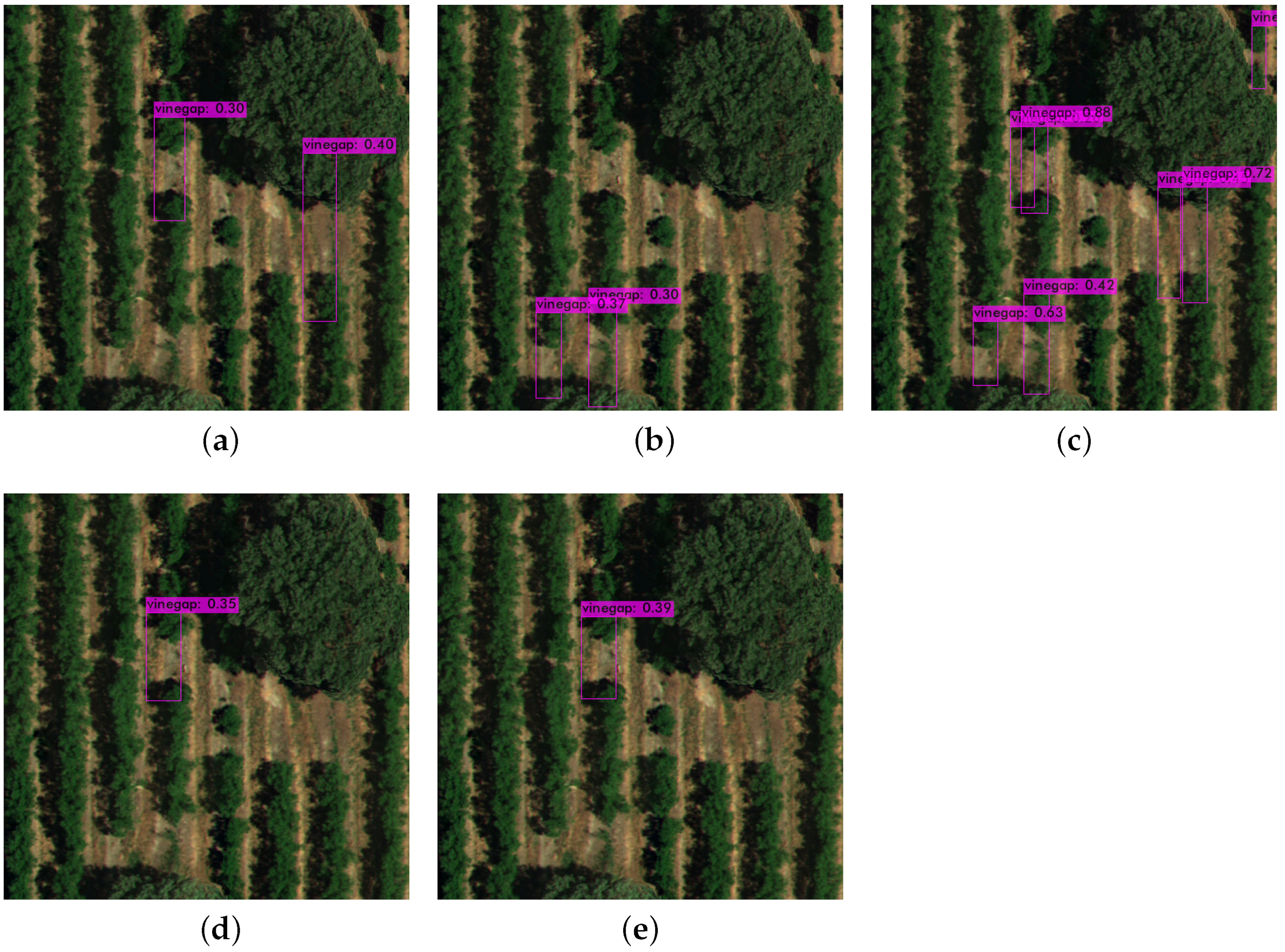
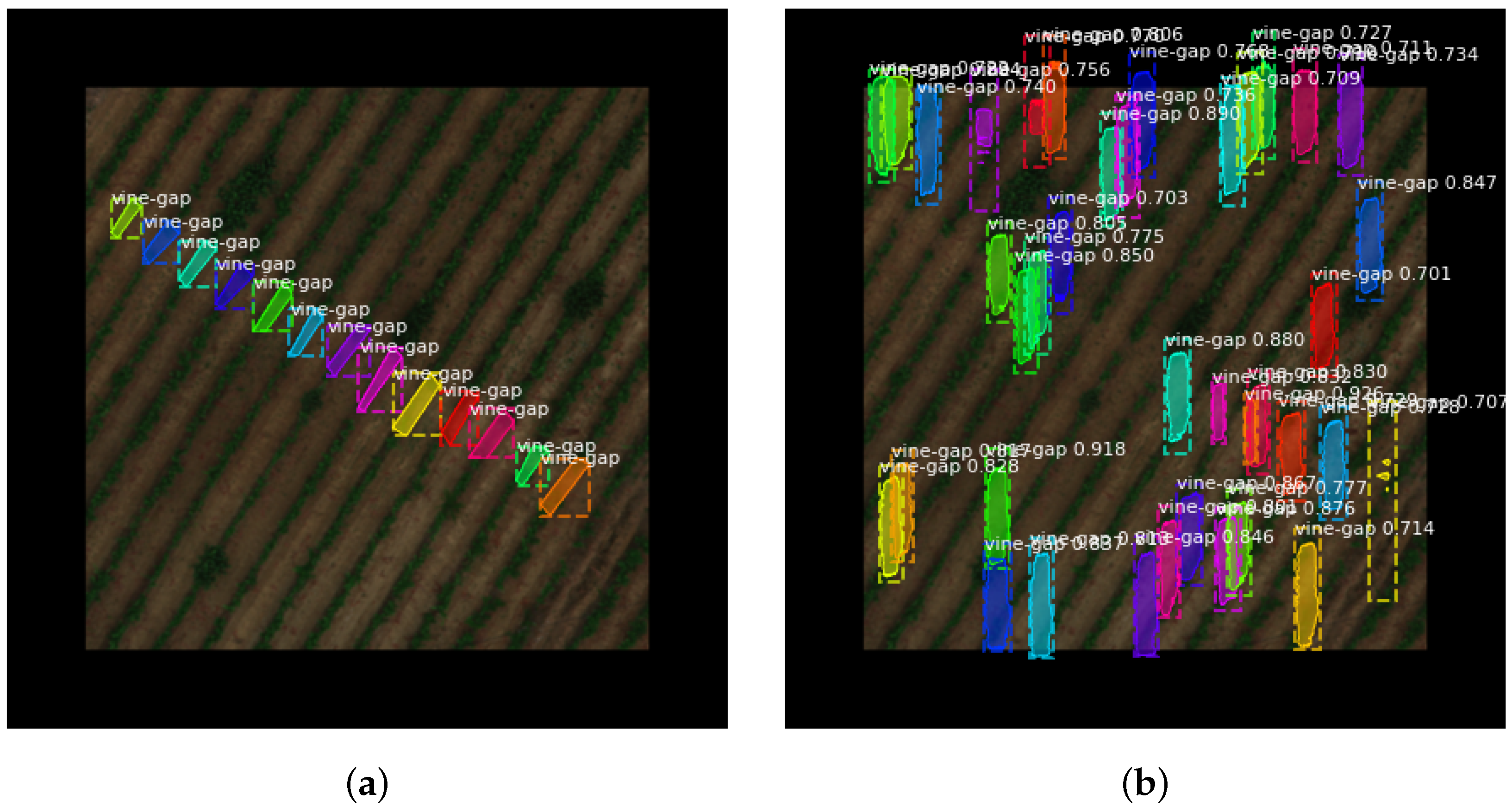
The results observed by passing the test images through each network, and different weights, show that the confidence values usually are higher in Tiny-YOLOv4, which is the network that gave the best results overall—consistently above 30%. he other networks returned more inconsistent values (between 10% and 80%) with more false positives. However, this is not how it evolved when looking at each individual dataset. Sometimes, confidence values increased and decreased from network to network; for example, in Figure 4, the confidence values seem to increase from Tiny-YOLOv3 to Tiny-YOLOv4 but decrease slightly from Tiny-YOLOv2 to Tiny-YOLOv3. This of course is not consistent with all detections but an overall observation after looking at a random set of images from the test dataset. The NDRE and NDWI datasets started the worst with none to very few detections in the random set, from Tiny-YOLO and YOLO, which could be expected, since those were not able to achieve an $A{P}_{50}$ above 45%. Slight increases in detections were observed with the latter networks, Tiny-YOLOv3 and Tiny-YOLOv4; and at this point, two detections of the same gap became rare unlike with the previous networks. There were not found at any point, in this random test set, situations where the networks categorized a path as a gap, but other errors occurred: as seen in Figure 4, sometimes trees confused the networks into believing there were gaps.

4.2. Results of Training Mask-RCNN ‘head’ Layers

After training all regression-based networks individually, the region-based network was trained, Mask-RCNN. Since there were already 30 weights from the previous round of training from all the regression networks, for each dataset, those were the optimal starting weights to use in the next two rounds.

The scripts used to convert the weights files into h5 files to use for training Mask-RCNN were [67] for YOLO, Tiny-YOLO, and Tiny-YOLOv2 weights; Ref. [68] for Tiny-YOLOv3 weights; and [69] for Tiny-YOLOv4 weights. Furthermore, using the hardware previously mentioned, it was only possible to train the ‘heads’ of the Mask-RCNN network, which included the RPN, classifier, and mask head layers.

The hardware used in training the results presented in Table 4 was again the computer with an Intel^® Core™ i7-9750H CPU @ 2.60 GHz × 12 processor and a NVIDIA GeForce GTX 1660 Ti/PCIe/SSE2 graphics card, and Google Colab [70] was used for time management purposes.

By looking at Table 4, one can conclude that the best dataset for this stage of training was the GS dataset, and the best outcome came from training Mask-RCNN with weights from Tiny-YOLOv3. In this initial training stage, the AP values were expected to be small, due to the smaller number of epochs, and since the only layers being trained were the ’head’ layers, most of the layers were not trained. In conclusion, only training the ’head’ layers was not enough for obtaining good AP, similar to the values in Table 3. When it came to the best starting weights for training, they did not follow the previous results in Table 3, since Tiny-YOLOv4 did not perform as well and Tiny-YOLOv3 performed the best. This could have been due to different conversions of the weight files, due to the different architectures, which could heavily have influenced the first 30 epochs of training.

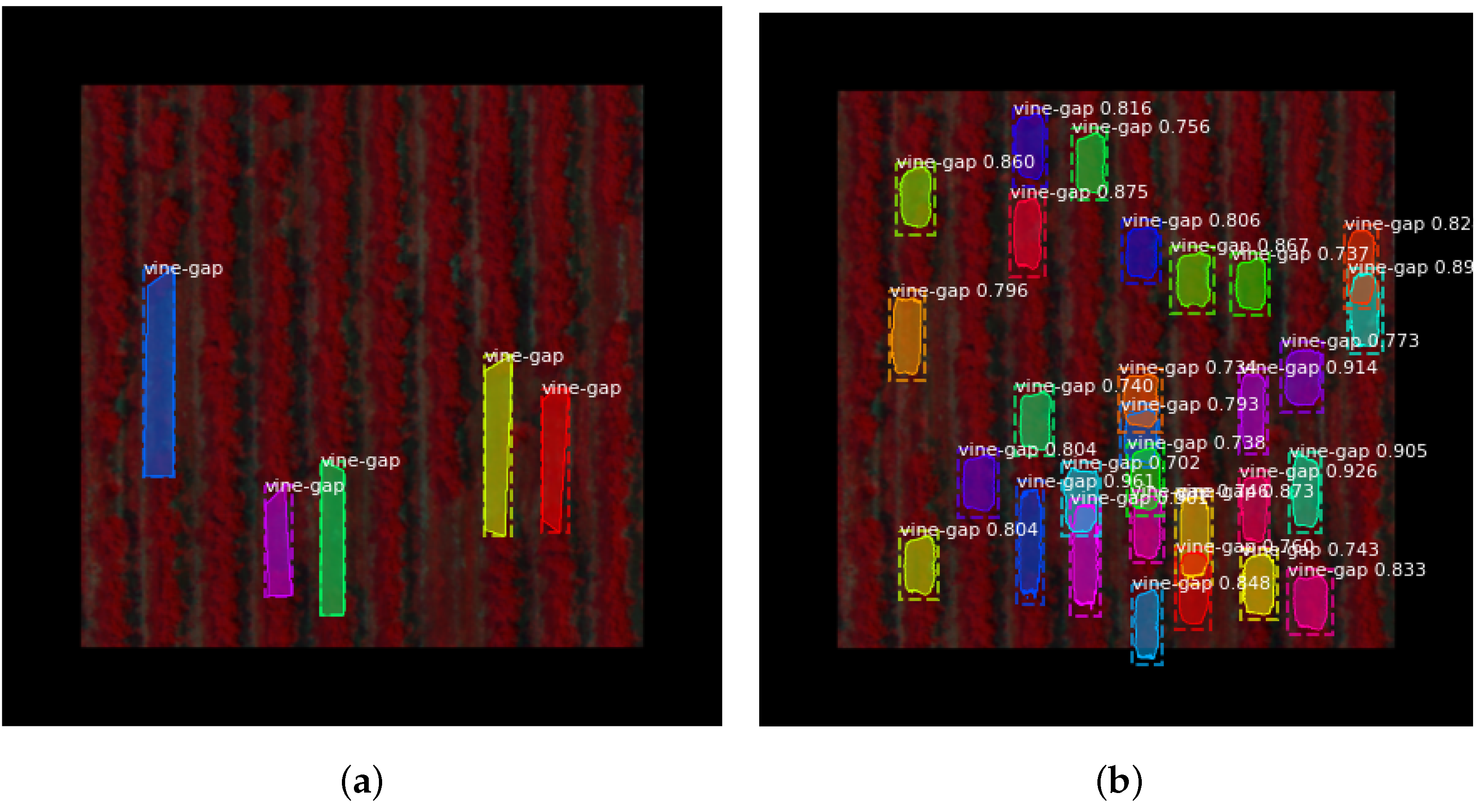
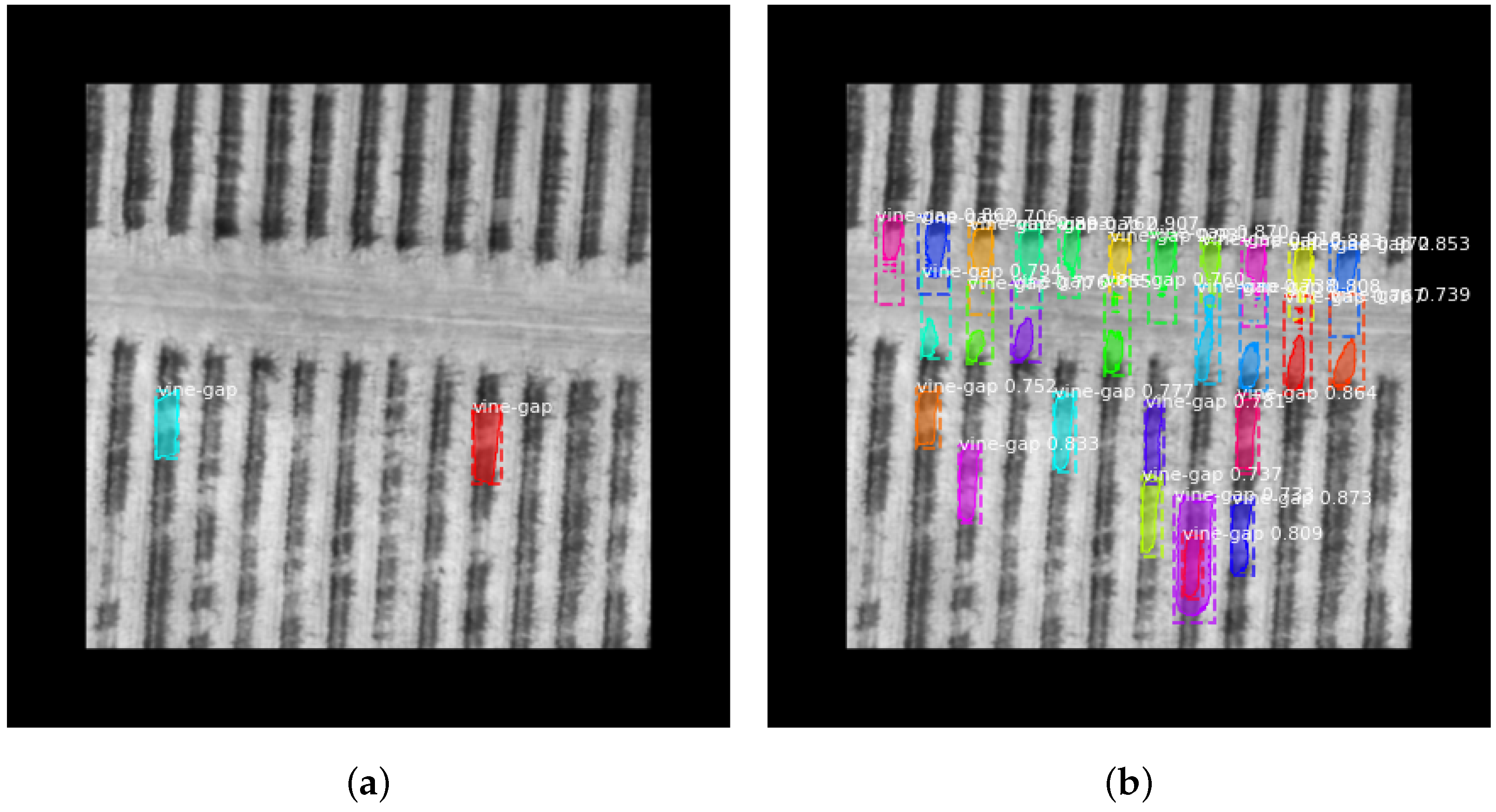
At this point in training, some common issues arose that were expected to go away or diminish by the time Mask-RCNN finished the second stage of training. By looking at Figure 5, it can be seen that the exit of the network usually detects more and smaller gaps than those marked; this is not particularly a bad thing, but is indicative of the fact that most marked gaps are smaller in size. At this point in testing the network still did not differentiate between paths and actual plantation gaps, this was particularly difficult to get rid of since, as seen in Figure 6, these paths sometimes are very similar to gaps.

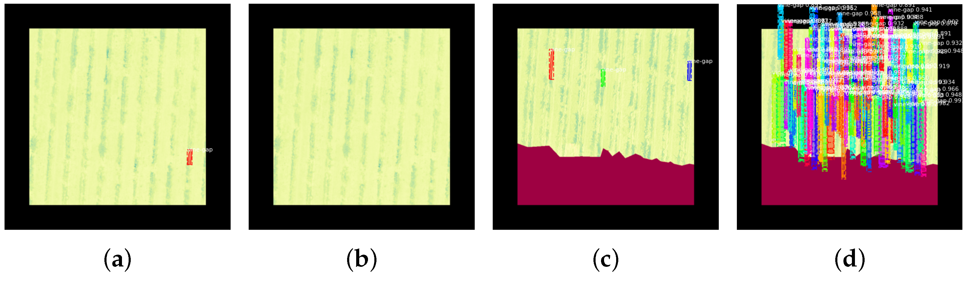
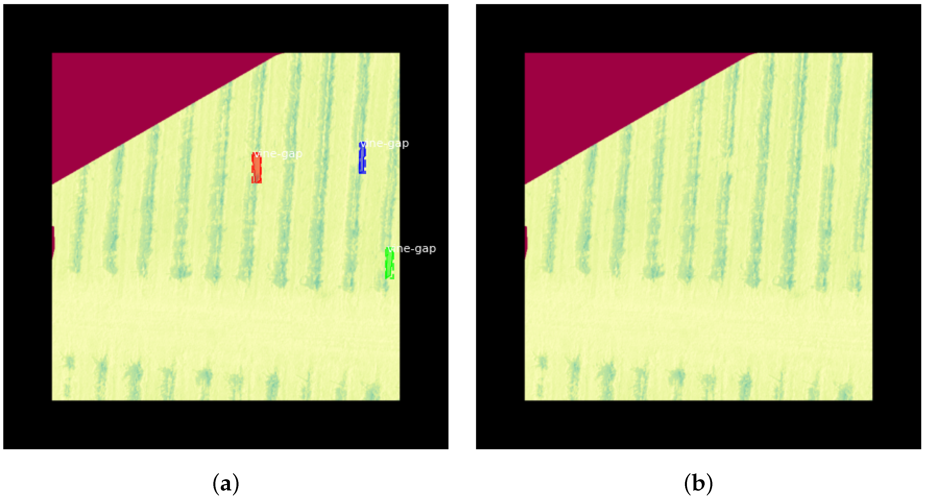
Some datasets, such as NDRE, NDVI, and NDWI, also tended to either have too many detected gaps or none at all, as seen in Figure 7. There could be two ways of looking at it: the first and the one that probably has more influence on the results is the smaller amount of training images; the other is that these images have generally less contrast, which can either lead to nothing being detected or everything being detected as a gap.

At this point, the network seems to also be mostly incapable of detecting the gaps that are closer to 45º in orientation, as seen in Figure 8. This is due to the decreased amount of images, with crops being displayed diagonally in the dataset and the training time being only 30 epochs.

4.3. Results of Training Mask-RCNN ‘all’ Layers

At this point, as mentioned previously in Section 3.1, new images were added to some of the datasets (see Table 1 and Table 2), so the dataset images were once again shuffled using Algorithm 2 into the train or test sets before training.

The hardware used in training the networks presented in Table 5 was a computer with a processor Intel^® Core™ i7-8700 CPU @ 3.20 GHz × 12 and a graphics card GeForce RTX 2070 SUPER/PCIe/SSE2. The computer was changed because the code could not run in the previous one due to the GPU not being able to complete the training and crashing.

The subsequent fine-tuning results presented in Table 5 infer that the best dataset in this stage was the RGB dataset, and the best starting weights for Mask-RCNN were the weights from Tiny-YOLO. At this point in training, some of the issues discussed in the previous stage of training should be expected to be diminished. There were no issues related to the prediction of too many gaps in an image observed, as discussed previously and presented in Figure 7, although, sometimes, as seen in Figure 9, there were cases where no objects were detected.

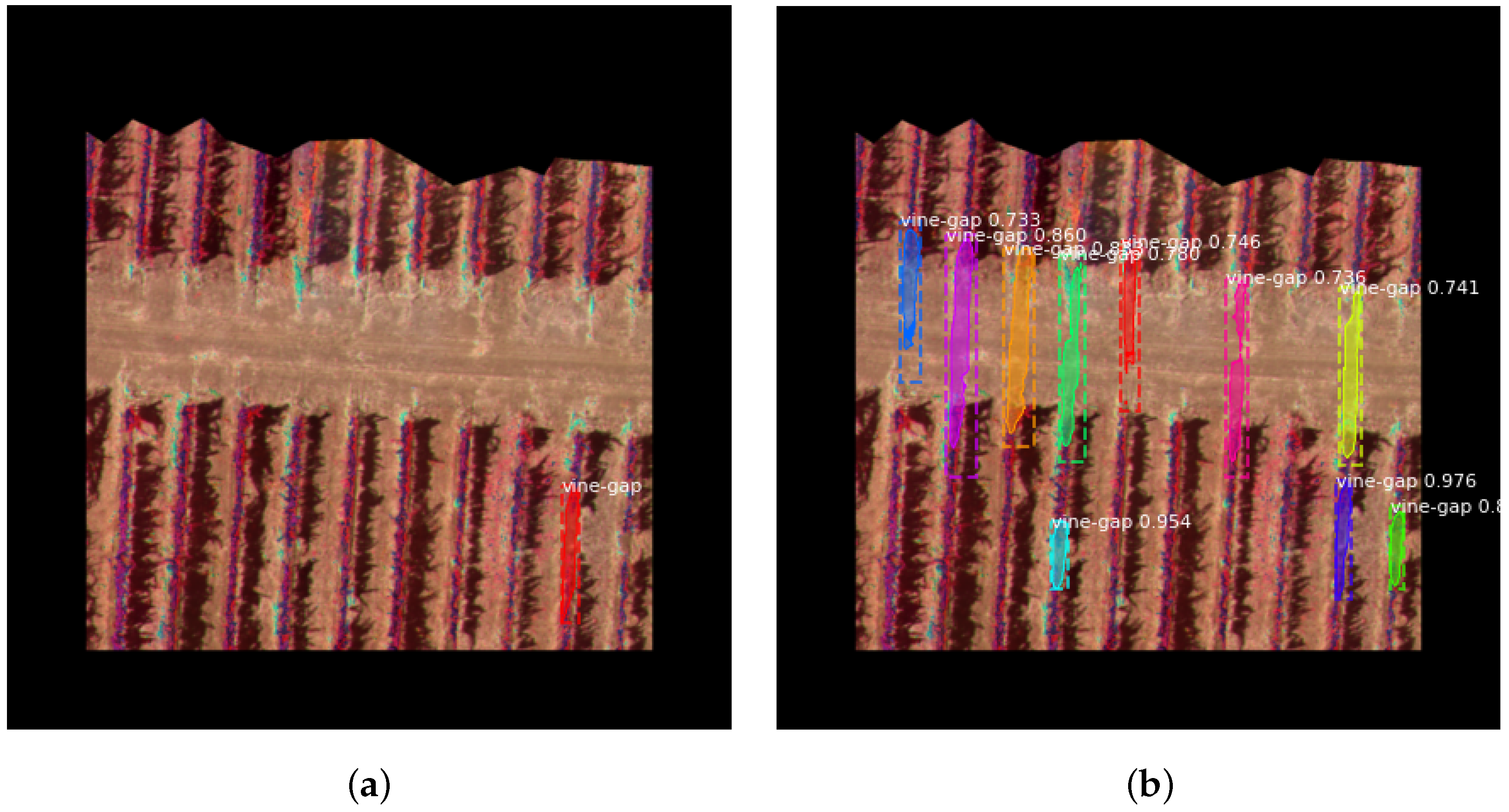
Another situation where the network does not work properly is when the network still detects objects in paths, although, this time, the predicted regions are bigger, as seen in Figure 10. The number of predictions is multiple times greater than the number of ground truth boxes, this is not a big problem since, as discussed previously, not every gap was marked, and the extra predictions made can be categorized as gaps with minimal vegetation, although not being fully empty of vegetation. This affects the $AP$, since the accuracy is calculated about truth bounding boxes, if there are extra prediction boxes than those seen as erroneous by the accuracy calculation algorithm.

5. Discussion

After training all networks with each dataset and analyzing the results from the regression-based networks, it was concluded that the best network was Tiny-YOLOv4, as a possible solution for depletion in a UAV. The weights of Tiny-YOLO were the best as starting weights for Mask-RCNN, which also performed well in detecting the different polygon regions that encapsulated the different gaps, after the second stage of training. The different networks also were able to detect additional gaps beside the ones in ground truth boxes, which were not found in the test images of a predicted box encapsulating vegetation. More common were false positives where the networks identified roads, and spaces between the crops and trees as gaps in the plantation. The best dataset was the RGB dataset, although it is important to note that the datasets were not balanced. It is not possible to conclusively say that this is the best dataset, since it is also the biggest of all of them, sometimes with thousands more images than some of the others. This severely affects the end results, since this dataset also has more training data, so the networks can better approximate in those cases.

A comment must be made about the labeling of the different polygons, since the labeling was entirely done by one person. This is not ideal, since it leads to fewer ground truth boxes being identified due to time constraints and human error. These situations are better avoided with more than one person being responsible for identifying ground truth boxes.

Analyzing

Table 6. The best results in each AP from each round of training and testing (Table 3, Table 4 and Table 5).

Method	Train	${\mathit{AP}}_{50}$	${\mathit{AP}}_{75}$
Tiny-YOLOv4	RGB	61.47%	19.62%
YOLO + Mask-RCNN (just ‘head’ layers)	NDVI	45.65%	6.88%
Tiny-YOLOv3 + Mask-RCNN (just ‘head’ layers)	GS	46.48%	6.48%
Tiny-YOLO + Mask-RCNN (full)	RGB	60.88%	12.81%
Tiny-YOLOv2 + Mask-RCNN (full)	RGB	59.10%	15.33%

showed that the best overall result was the solution with Tiny-YOLOv4 and an RGB dataset. Both these results coincided with our expectations, since [20] mentioned that the Tiny-YOLO version did not match YOLO in accuracy, so YOLO being better than Tiny-YOLO was expected; for the rest, since every subsequent YOLO version managed to improve on its predecessor, it was expected that, even for Tiny versions they would follow an order of most recent to oldest YOLO. When it came to training Mask-RCNN, the best result was with starting weights from Tiny-YOLO, after training a combined of 80 epochs (30 epochs for head layers and 50 for all layers). As discussed in previous chapters and sections, the results most probably were influenced by the amount of data inside each dataset, being that RGB was the biggest dataset. Due to the different dataset sizes, it is not possible to ensure which dataset performs better overall. To enable it, it is necessary to recreate the conditions using the same amount of training and testing data to be able to directly compare which image format performs best.

6. Conclusions

In this paper, multiple regression-based networks—YOLO, Tiny-YOLO, Tiny-YOLOv2, Tiny-YOLOv3, and Tiny-YOLOv4—were trained with different datasets comprised of maps made from different multi-spectral indexes, in order to determine which combination resulted in the best network to be employed in a drone for detection of gaps in a vine plantation. Besides the regression-based networks mentioned, Mask-RCNN was trained with the weights resulting from the regression-based training sessions, with the respective datasets.

This study was an initial attempt at resolving the issue of plantation gap detection using UAV imagery. One issue that still is unresolved is the false positives detected in paths, which are very similar to gaps. The false positives can be diminished by training the networks for a longer period but, since not every gap was labeled, this would teach the networks to ignore smaller or low-vegetation gaps most of the time. Future improvements include a better dataset with all data labeled correctly, which can be achieved using the final weights in this study, and later removing any incorrect identification. Having this dataset would mean that the networks could be trained for longer periods of time without learning to ignore less obvious gaps.

With this research, the work presented can continue by generalizing these networks to detect more than gaps. By using multi-spectral images, the system can also be trained into detecting parts of the crops where the vegetation is drier and use that information to control the irrigation system in order to avoid watering gaps and places where the plants and soil still have acceptable levels of humidity. The supervision of humidity in a certain field can be done with NDWI and NDVI images with the help of UAV imagery, as seen in [71].

Further studies could be made where the different variables are diminished or erased, or new studies focused on different types of agricultural issues could continue from here, where the best multi-spectral indexes, image formats, and networks can be determined and employed into a drone as solutions.

References

- Kummu, M.; Taka, M.; Guillaume, J.H. Gridded Global Datasets for Gross Domestic Product and Human Development Index over 1990–2015; Nature Publishing Group: Berlin, Germany, 2018; Volume 5, pp. 1–15. [Google Scholar] [CrossRef]
- Tang, Y.; Luan, X.; Sun, J.; Zhao, J.; Yin, Y.; Wang, Y.; Sun, S. Impact assessment of climate change and human activities on GHG emissions and agricultural water use. Agric. For. Meteorol. 2021, 296, 108218. [Google Scholar] [CrossRef]
- Jensen, C.; Ørum, J.E.; Pedersen, S.; Andersen, M.; Plauborg, F.; Liu, F.; Jacobsen, S.E. A Short Overview of Measures for Securing Water Resources for Irrigated Crop Production. J. Agron. Crop Sci. 2014, 200, 333–343. [Google Scholar] [CrossRef]
- Mestre, G.; Matos-Carvalho, J.P.; Tavares, R.M. Irrigation Management System using Artificial Intelligence Algorithms. In Proceedings of the 2022 International Young Engineers Forum (YEF-ECE), Lisbon, Portugal, 1 July 2022; pp. 69–74. [Google Scholar] [CrossRef]
- Tsouros, D.C.; Bibi, S.; Sarigiannidis, P.G. A review on UAV-based applications for precision agriculture. Information 2019, 10, 349. [Google Scholar] [CrossRef]
- Merz, M.; Pedro, D.; Skliros, V.; Bergenhem, C.; Himanka, M.; Houge, T.; Matos-Carvalho, J.P.; Lundkvist, H.; Cürüklü, B.; Hamrén, R.; et al. Autonomous UAS-Based Agriculture Applications: General Overview and Relevant European Case Studies. Drones 2022, 6, 128. [Google Scholar] [CrossRef]
- Pedro, D.; Lousã, P.; Ramos, Á.; Matos-Carvalho, J.P.; Azevedo, F.; Campos, L. HEIFU—Hexa Exterior Intelligent Flying Unit. In Proceedings of the Computer Safety, Reliability, and Security, SAFECOMP 2021 Workshops, York, UK, 7 September 2021; Habli, I., Sujan, M., Gerasimou, S., Schoitsch, E., Bitsch, F., Eds.; Springer International Publishing: Cham, Switzerland, 2021; pp. 89–104. [Google Scholar]
- Correia, S.; Realinho, V.; Braga, R.; Turégano, J.; Miranda, A.; Gañan, J. Development of a Monitoring System for Efficient Management of Agricultural Resources. In Proceedings of the VIII International Congress on Project Engineering, Bilbao, Spain, 7–8 October 2004; pp. 1215–1222. [Google Scholar]
- Torky, M.; Hassanein, A.E. Integrating blockchain and the internet of things in precision agriculture: Analysis, opportunities, and challenges. Comput. Electron. Agric. 2020, 178, 105476. [Google Scholar] [CrossRef]
- Sishodia, R.P.; Ray, R.L.; Singh, S.K. Applications of remote sensing in precision agriculture: A review. Remote Sens. 2020, 12, 3136. [Google Scholar] [CrossRef]
- Charu, C.A. Neural Networks and Deep Learning: A Textbook; Determination Press: San Francisco, CA, USA, 2018. [Google Scholar]
- Henrique, A.S.; Fernandes, A.M.R.; Rodrigo, L.; Leithardt, V.R.Q.; Correia, S.D.; Crocker, P.; Scaranto Dazzi, R.L. Classifying Garments from Fashion-MNIST Dataset Through CNNs. Adv. Sci. Technol. Eng. Syst. J. 2021, 6, 989–994. [Google Scholar] [CrossRef]
- Matos-Carvalho, J.P.; Santos, R.; Tomic, S.; Beko, M. GTRS-Based Algorithm for UAV Navigation in Indoor Environments Employing Range Measurements and Odometry. IEEE Access 2021, 9, 89120–89132. [Google Scholar] [CrossRef]
- Santos, R.; Matos-Carvalho, J.P.; Tomic, S.; Beko, M.; Correia, S.D. Applying Deep Neural Networks to Improve UAV Navigation in Satellite-less Environments. In Proceedings of the 2022 International Young Engineers Forum (YEF-ECE), Lisbon, Portugal, 1 July 2022; pp. 63–68. [Google Scholar] [CrossRef]
- Santos, R.; Matos-Carvalho, J.P.; Tomic, S.; Beko, M. WLS algorithm for UAV navigation in satellite-less environments. IET Wirel. Sens. Syst. 2022, 12, 93–102. [Google Scholar] [CrossRef]
- Salazar, L.H.A.; Leithardt, V.R.; Parreira, W.D.; da Rocha Fernandes, A.M.; Barbosa, J.L.V.; Correia, S.D. Application of Machine Learning Techniques to Predict a Patient’s No-Show in the Healthcare Sector. Future Internet 2022, 14, 3. [Google Scholar] [CrossRef]
- Ramesh, N.V.K.; B, M.R.; B, B.D.; Suresh, N.; Rao, K.R.; Reddy, B.N.K. Identification of Tomato Crop Diseases Using Neural Networks-CNN. In Proceedings of the 2021 12th International Conference on Computing Communication and Networking Technologies (ICCCNT), Kharagpur, India, 6–8 July 2021; pp. 1–5. [Google Scholar] [CrossRef]
- Narvekar, C.; Rao, M. Flower classification using CNN and transfer learning in CNN- Agriculture Perspective. In Proceedings of the 2020 3rd International Conference on Intelligent Sustainable Systems (ICISS), Thoothukudi, India, 3–5 December 2020; pp. 660–664. [Google Scholar] [CrossRef]
- Salvado, A.B.; Mendonça, R.; Lourenço, A.; Marques, F.; Matos-Carvalho, J.P.; Miguel Campos, L.; Barata, J. Semantic Navigation Mapping from Aerial Multispectral Imagery. In Proceedings of the 2019 IEEE 28th International Symposium on Industrial Electronics (ISIE), Vancouver, BC, Canada, 12–14 June 2019; pp. 1192–1197. [Google Scholar] [CrossRef]
- Redmon, J.; Divvala, S.; Girshick, R.; Farhadi, A. You Only Look Once: Unified, Real-Time Object Detection. In Proceedings of the 2016 IEEE Conference on Computer Vision and Pattern Recognition (CVPR), Las Vegas, NV, USA, 27–30 June 2016; pp. 779–788. [Google Scholar] [CrossRef]
- He, K.; Gkioxari, G.; Dollár, P.; Girshick, R. Mask r-cnn. In Proceedings of the IEEE International Conference on Computer Vision, Venice, Italy, 22–29 October 2017; pp. 2961–2969. [Google Scholar]
- Girshick, R.; Donahue, J.; Darrell, T.; Malik, J. Rich feature hierarchies for accurate object detection and semantic segmentation. In Proceedings of the IEEE Conference on Computer Vision and Pattern Recognition, Columbus, OH, USA, 23–28 June 2014; pp. 580–587. [Google Scholar]
- Ren, S.; He, K.; Girshick, R.; Sun, J. Faster r-cnn: Towards real-time object detection with region proposal networks. Adv. Neural Inf. Process. Syst. 2015, 28, 1–14. [Google Scholar] [CrossRef] [PubMed]
- Gao, B.C. NDWI—A normalized difference water index for remote sensing of vegetation liquid water from space. Remote Sens. Environ. 1996, 58, 257–266. [Google Scholar] [CrossRef]
- Mozgeris, G.; Gadal, S.; Jonikavičius, D.; Straigytė, L.; Ouerghemmi, W.; Juodkienė, V. Hyperspectral and color-infrared imaging from ultralight aircraft: Potential to recognize tree species in urban environments. In Proceedings of the 2016 8th Workshop on Hyperspectral Image and Signal Processing: Evolution in Remote Sensing (WHISPERS), Los Angeles, CA, USA, 21–24 August 2016; pp. 1–5. [Google Scholar]
- Boiarskii, B.; Hasegawa, H. Comparison of NDVI and NDRE Indices to Detect Differences in Vegetation and Chlorophyll Content. J. Mech. Contin. Math. Sci. 2019, spl1. [Google Scholar] [CrossRef]
- Yagci, A.L.; Di, L.; Deng, M. The influence of land cover-related changes on the NDVI-based satellite agricultural drought indices. In Proceedings of the 2014 IEEE Geoscience and Remote Sensing Symposium, Quebec City, QC, Canada, 13–18 July 2014; pp. 2054–2057. [Google Scholar]
- Subba Rao, V.P.; Rao, G.S. Design and Modelling of anAffordable UAV Based Pesticide Sprayer in Agriculture Applications. In Proceedings of the 2019 Fifth International Conference on Electrical Energy Systems (ICEES), Chennai, India, 21–22 February 2019; pp. 1–4. [Google Scholar] [CrossRef]
- Zheng, H.; Zhou, X.; Cheng, T.; Yao, X.; Tian, Y.; Cao, W.; Zhu, Y. Evaluation of a UAV-based hyperspectral frame camera for monitoring the leaf nitrogen concentration in rice. In Proceedings of the 2016 IEEE International Geoscience and Remote Sensing Symposium (IGARSS), Beijing, China, 10–15 July 2016; pp. 7350–7353. [Google Scholar] [CrossRef]
- Li, D.; Zheng, H.; Xu, X.; Lu, N.; Yao, X.; Jiang, J.; Wang, X.; Tian, Y.; Zhu, Y.; Cao, W.; et al. BRDF Effect on the Estimation of Canopy Chlorophyll Content in Paddy Rice from UAV-Based Hyperspectral Imagery. In Proceedings of the IGARSS 2018—2018 IEEE International Geoscience and Remote Sensing Symposium, Valencia, Spain, 22–27 July 2018; pp. 6464–6467. [Google Scholar] [CrossRef]
- Matos-Carvalho, J.P.; Pedro, D.; Campos, L.M.; Fonseca, J.M.; Mora, A. Terrain Classification Using W-K Filter and 3D Navigation with Static Collision Avoidance. In Proceedings of the SAI Intelligent Systems Conference, London, UK, 5–6 September 2019; Bi, Y., Bhatia, R., Kapoor, S., Eds.; Springer International Publishing: Cham, Switzerland, 2020; pp. 1122–1137. [Google Scholar]
- Vardhini, P.; Asritha, S.; Devi, Y. Efficient Disease Detection of Paddy Crop using CNN. In Proceedings of the 2020 International Conference on Smart Technologies in Computing, Electrical and Electronics (ICSTCEE), Bengaluru, India, 9–10 October 2020; pp. 116–119. [Google Scholar] [CrossRef]
- Feng, Q.; Chen, J.; Li, X.; Li, C.; Wang, X. Multi-spectral Image Fusion Method for Identifying Similar-colored Tomato Organs. In Proceedings of the 2019 IEEE International Conference on Unmanned Systems and Artificial Intelligence (ICUSAI), Shenzhen, China, 21–23 April 2019; pp. 142–145. [Google Scholar] [CrossRef]
- Zhou, Z.; Li, S.; Shao, Y. Crops Classification from Sentinel-2A Multi-spectral Remote Sensing Images Based on Convolutional Neural Networks. In Proceedings of the IGARSS 2018–2018 IEEE International Geoscience and Remote Sensing Symposium, Valencia, Spain, 22–27 July 2018; pp. 5300–5303. [Google Scholar] [CrossRef]
- Hossain, M.I.; Paul, B.; Sattar, A.; Islam, M.M. A Convolutional Neural Network Approach to Recognize the Insect: A Perspective in Bangladesh. In Proceedings of the 2019 8th International Conference System Modeling and Advancement in Research Trends (SMART), Moradabad, India, 22–23 November 2019; pp. 384–389. [Google Scholar] [CrossRef]
- Murata, K.; Ito, A.; Takahashi, Y.; Hatano, H. A Study on Growth Stage Classification of Paddy Rice by CNN using NDVI Images. In Proceedings of the 2019 Cybersecurity and Cyberforensics Conference (CCC), Melbourne, Australia, 8–9 May 2019; pp. 85–90. [Google Scholar] [CrossRef]
- Habibie, M.I.; Ahamed, T.; Noguchi, R.; Matsushita, S. Deep Learning Algorithms to determine Drought prone Areas Using Remote Sensing and GIS. In Proceedings of the 2020 IEEE Asia-Pacific Conference on Geoscience, Electronics and Remote Sensing Technology (AGERS), Jakarta, Indonesia, 7–8 December 2020; pp. 69–73. [Google Scholar] [CrossRef]
- Sobayo, R.; Wu, H.H.; Ray, R.; Qian, L. Integration of Convolutional Neural Network and Thermal Images into Soil Moisture Estimation. In Proceedings of the 2018 1st International Conference on Data Intelligence and Security (ICDIS), South Padre Island, TX, USA, 8–10 April 2018; pp. 207–210. [Google Scholar] [CrossRef]
- Liu, Z.; Wu, J.; Fu, L.; Majeed, Y.; Feng, Y.; Li, R.; Cui, Y. Improved Kiwifruit Detection Using Pre-Trained VGG16 With RGB and NIR Information Fusion. IEEE Access 2020, 8, 2327–2336. [Google Scholar] [CrossRef]
- Dalal, N.; Triggs, B. Histograms of oriented gradients for human detection. In Proceedings of the 2005 IEEE Computer Society Conference on Computer Vision and Pattern Recognition (CVPR’05), San Diego, CA, USA, 20–25 June 2005; Volume 1, pp. 886–893. [Google Scholar] [CrossRef]
- Wang, X.; Zhuang, X.; Zhang, W.; Chen, Y.; Li, Y. Lightweight Real-time Object Detection Model for UAV Platform. In Proceedings of the 2021 International Conference on Computer Communication and Artificial Intelligence (CCAI), Guangzhou, China, 7–9 May 2021; pp. 20–24. [Google Scholar] [CrossRef]
- Gotthans, J.; Gotthans, T.; Marsalek, R. Prediction of Object Position from Aerial Images Utilising Neural Networks. In Proceedings of the 2021 31st International Conference Radioelektronika (RADIOELEKTRONIKA), Brno, Czech Republic, 19–21 April 2021; pp. 1–5. [Google Scholar] [CrossRef]
- Ding, Y.; Qu, Y.; Zhang, Q.; Tong, J.; Yang, X.; Sun, J. Research on UAV Detection Technology of Gm-APD Lidar Based on YOLO Model. In Proceedings of the 2021 IEEE International Conference on Unmanned Systems (ICUS), Beijing, China, 22–24 October 2021; pp. 105–109. [Google Scholar] [CrossRef]
- Redmon, J.; Farhadi, A. YOLO9000: Better, Faster, Stronger. In Proceedings of the 2017 IEEE Conference on Computer Vision and Pattern Recognition (CVPR), Honolulu, HI, USA, 21–26 July 2017; pp. 6517–6525. [Google Scholar] [CrossRef]
- Redmon, J.; Farhadi, A. Yolov3: An incremental improvement. arXiv 2018, arXiv:1804.02767. [Google Scholar]
- Bochkovskiy, A.; Wang, C.; Liao, H.M. YOLOv4: Optimal Speed and Accuracy of Object Detection. CoRR 2020. Available online: http://xxx.lanl.gov/abs/2004.10934 (accessed on 1 October 2021).
- Girshick, R. Fast r-cnn. In Proceedings of the IEEE International Conference on Computer Vision, Santiago, Chile, 7–13 December 2015. pp. 1440–1448.
- Srinivas, R.; Nithyanandan, L.; Umadevi, G.; Rao, P.V.V.S.; Kumar, P.N. Design and implementation of S-band Multi-mission satellite positioning data simulator for IRS satellites. In Proceedings of the 2011 IEEE Applied Electromagnetics Conference (AEMC), Kolkata, India, 18–22 December 2011; pp. 1–4. [Google Scholar] [CrossRef]
- Weidong, Z.; Chun, W.; Jing, H. Development of agriculture machinery aided guidance system based on GPS and GIS. In Proceedings of the 2010 World Automation Congress, Kobe, Japan, 19–23 September 2010; pp. 313–317. [Google Scholar]
- Yu, H.; Liu, Y.; Yang, G.; Yang, X. Quick image processing method of HJ satellites applied in agriculture monitoring. In Proceedings of the 2016 World Automation Congress (WAC), Rio Grande, Puerto Rico, 31 July–4 August 2016; pp. 1–5. [Google Scholar] [CrossRef]
- Murugan, D.; Garg, A.; Ahmed, T.; Singh, D. Fusion of drone and satellite data for precision agriculture monitoring. In Proceedings of the 2016 11th International Conference on Industrial and Information Systems (ICIIS), Roorkee, India, 3–4 December 2016; pp. 910–914. [Google Scholar] [CrossRef]
- Bansod, B.; Singh, R.; Thakur, R.; Singhal, G. A comparision between satellite based and drone based remote sensing technology to achieve sustainable development: A review. J. Agric. Environ. Int. Dev. (JAEID) 2017, 111, 383–407. [Google Scholar]
- Shao, L.; Zhu, F.; Li, X. Transfer Learning for Visual Categorization: A Survey. IEEE Trans. Neural Netw. Learn. Syst. 2015, 26, 1019–1034. [Google Scholar] [CrossRef]
- Chiba, S.; Sasaoka, H. Basic Study for Transfer Learning for Autonomous Driving in Car Race of Model Car. In Proceedings of the 2021 6th International Conference on Business and Industrial Research (ICBIR), Bangkok, Thailand, 20–21 May 2021; pp. 138–141. [Google Scholar] [CrossRef]
- Shenavarmasouleh, F.; Arabnia, H.R. DRDr: Automatic Masking of Exudates and Microaneurysms Caused by Diabetic Retinopathy Using Mask R-CNN and Transfer Learning. In Advances in Computer Vision and Computational Biology; Arabnia, H.R., Deligiannidis, L., Shouno, H., Tinetti, F.G., Tran, Q.N., Eds.; Springer International Publishing: Cham, Switzerland, 2021; pp. 307–318. [Google Scholar]
- Khan, M.A.; Akram, T.; Zhang, Y.D.; Sharif, M. Attributes based skin lesion detection and recognition: A mask RCNN and transfer learning-based deep learning framework. Pattern Recognit. Lett. 2021, 143, 58–66. [Google Scholar] [CrossRef]
- Wani, M.A.; Afzal, S. A New Framework for Fine Tuning of Deep Networks. In Proceedings of the 2017 16th IEEE International Conference on Machine Learning and Applications (ICMLA), Cancun, Mexico, 18–21 December 2017; pp. 359–363. [Google Scholar] [CrossRef]
- Too, E.C.; Yujian, L.; Njuki, S.; Yingchun, L. A comparative study of fine-tuning deep learning models for plant disease identification. Comput. Electron. Agric. 2019, 161, 272–279. [Google Scholar] [CrossRef]
- AlexeyAB. Darknet. Github Repository. Available online: https://github.com/AlexeyAB/darknet (accessed on 1 November 2021).
- matterport. Mask RCNNGithub Repository. Available online: https://github.com/matterport/Mask_RCNN (accessed on 1 November 2021).
- RedEdge-MX Integration Guide. 2022. Available online: https://support.micasense.com/hc/en-us/articles/360011389334-RedEdge-MX-Integration-Guide (accessed on 1 November 2022).
- Pino, M.; Matos-Carvalho, J.P.; Pedro, D.; Campos, L.M.; Costa Seco, J. UAV Cloud Platform for Precision Farming. In Proceedings of the 2020 12th International Symposium on Communication Systems, Networks and Digital Signal Processing (CSNDSP), Porto, Portugal, 20–22 July 2020; pp. 1–6. [Google Scholar] [CrossRef]
- Vong, A.; Matos-Carvalho, J.P.; Toffanin, P.; Pedro, D.; Azevedo, F.; Moutinho, F.; Garcia, N.C.; Mora, A. How to Build a 2D and 3D Aerial Multispectral Map?—All Steps Deeply Explained. Remote Sens. 2021, 13, 3227. [Google Scholar] [CrossRef]
- AlexeyAB. Yolo Mark. Github Repository. Available online: https://github.com/AlexeyAB/Yolo_mark (accessed on 1 November 2021).
- Dutta, A.; Zisserman, A. The VIA Annotation Software for Images, Audio and Video. In Proceedings of the 27th ACM International Conference on Multimedia, Nice, France, 21–25 October 2019; ACM: New York, NY, USA, 2019. [Google Scholar] [CrossRef]
- Michelucci, U. Advanced Applied Deep Learning: Convolutional Neural Networks and Object Detection; Apress: Pune, India, 2019. [Google Scholar] [CrossRef]
- Allanzelener. YAD2K: Yet Another Darknet 2 Keras. Github Repository. Available online: https://github.com/allanzelener/YAD2K (accessed on 1 November 2021).
- Xiaochus. YOLOv3. Github Repository. Available online: https://github.com/xiaochus/YOLOv3 (accessed on 1 November 2021).
- Runist. YOLOv4. Github Repository. Available online: https://github.com/Runist/YOLOv4.git (accessed on 1 November 2021).
- Google. Google CoLaboratory. Available online: https://colab.research.google.com/drive/151805XTDg–dgHb3-AXJCpnWaqRhop_2#scrollTo=ojGuEt8MpJhA (accessed on 1 November 2021).
- Casamitjana, M.; Torres-Madroñero, M.C.; Bernal-Riobo, J.; Varga, D. Soil Moisture Analysis by Means of Multispectral Images According to Land Use and Spatial Resolution on Andosols in the Colombian Andes. Appl. Sci. 2020, 10, 5540. [Google Scholar] [CrossRef]
Figure 1.
Different image types of the same map. This figure includes the multispectral indices used (figures (a,d,e)) and the color image formats (figures (b,c)). (a) NDWI, (b) CIR, (c) RGB, (d) NDRE, and (e) NDVI.
Figure 2.
Manual identification of plantation gaps. As observed, we included parts of the vegetation inside the ground truth boxes (dashed line) and polygons (continuous line and colored areas).
Figure 3.
Example of cropped images from the same map in different multi-spectral indices. All 3 images share the same name in their respective datasets. (a) CIR, (b) NDWI, (c) RGB.
Figure 4.
Examples of regression-based networks’ results with predicted boxes from the respective networks, and confidence values for each object identified. Dataset: RGB; (a): Tiny-YOLO; (b): YOLO; (c): Tiny-YOLOv2; (d): Tiny-YOLOv3; (e): Tiny-YOLOv4.
Figure 5.
Examples of Mask-RCNN, after training ‘head’ layers for 30 epochs, detecting too many objects. Dataset: CIR; Weights: Tiny-YOLO; (a): Original; (b): Detected.
Figure 6.
Examples of Mask-RCNN, after training ‘head’ layers for 30 epochs, miscategorizing the path. Dataset: GS; Weights: Tiny-YOLO; (a): Original; (b): Detected.
Figure 7.
Examples of Mask-RCNN, after training ‘head’ layers for 30 epochs. Dataset: NDRE; Weights (a,b) YOLO; (c,d) Tiny-YOLOv2; (a,c): Original; (b,d): Detected. The Detected images (b,d) show two different network outputs in the same dataset and network. The image in (b) failed to detect the gap in (a), and the image in (d) predicted too many gaps in (c).
Figure 8.
Examples of Mask-RCNN, after training ‘head’ layers for 30 epochs, failing to detect diagonal objects. Dataset: RGB; Weights: Tiny-YOLOv2; (a): Original; (b): Detected.
Figure 9.
Examples of Mask-RCNN, after training ‘all’ layers for 50 epochs, failing to detect objects. Dataset: NDRE; Weights: YOLO; (a): original; (b): detected.
Figure 10.
Examples of Mask-RCNN, after training ‘all’ layers for 50 epochs, miscategorizing the path. Dataset: CIR; Weights: Tiny YOLOv4; (a): original; (b): detected.