A Simplified Algorithm for Dealing with Inconsistencies Using the Analytic Hierarchy Process

Abstract

Inconsistencies in the comparison matrix is a common problem in many studies using the analytic hierarchy process (AHP). While these may be identified and corrected through asking respondents to reconsider their choices, this is not always possible. This is particularly the case for online surveys, where the number of respondents may be large and often anonymous, such that interacting with individual respondents is neither feasible nor possible. Several approaches have previously been developed for autonomously adjusting the comparison matrix to deal with inconsistencies. In this paper, we build on these previous approaches, and present an algorithm that is conceptually and analytically simple and readily implementable in R. The algorithm is applied to several example cases to illustrate its performance, including an example case study involving data collected through a large online survey. The results suggest that the modified survey-derived comparison matrix derived using the algorithm produces consistent responses that do not substantially alter the individual preferences in most cases.

1. Introduction

The estimation of objective or criteria importance weights is an integral component of most multi-criteria decision analysis studies [1]. The analytic hierarchy process (AHP) [2,3] is a commonly applied approach for deriving such weights, e.g., [4,5,6,7]. The method estimates the relative importance of each criterion being assessed to different stakeholders or decision makers. The derived weights subsequently help determine which set of outcomes given a range of different management options may be overall most preferable to the different groups based on their preference sets.

AHP is based upon the construction of a series of comparison matrices, with each element of the matrix representing the relative importance of each criterion relative to another. From these comparison matrices, the set of criteria importance weights can be determined using a number of different approaches [8], as detailed in the following sections. The elements themselves are derived through stakeholders being required to compare and prioritize only two criteria at any one time. The pair-wise comparison used in the AHP method makes the process of assigning importance weights relatively easy for stakeholder respondents as only two sub-components are being compared at a time [1]. However, preference or importance weightings are highly subjective, and inconsistency is a common problem facing AHP, particularly when decision makers are confronted with many sets of comparisons [9]. For example, asked to consider three criteria through pairwise comparison, a stakeholder may rate A > B, B > C but C > A. This is an extreme outcome, known as a circular triad, but can and does occur in some cases. More often, we might find that the “implicit” relationship between, say C and A, in terms of the preference strength given the other prioritizations (i.e., A and B, B and C) differs from the stated relationship. The propensity for these inconsistencies to emerge increases with the number of criteria to be compared. The presence of inconsistency in the comparison matrix may result in issues such as the incorrect priority weighting associated with each of the attributes being considered [10]. When applied in a multi-criteria decision-making framework, these issues may result in incorrect ordering of management options, and the selection of a less-than-optimal option.

Inconsistency may arise for several reasons. Respondents do not necessarily cross check their responses, and even if they do, ensuring a perfectly consistent set of responses when many attributes are compared is difficult. The process of choosing a particular trade-off value can also depend on respondent’s attention, mood, feelings and mental efficiency [11], and inconsistencies may arise through essentially random errors created by variations in these respondent’s state of mind. The discrete nature of the 1-9 scale applied in AHP can also contribute to inconsistency, as a perfectly consistent response may require a fractional preference score [12]. Danner, et al. [13] found that excessive use of extreme values by respondents trying to highlight their strong preferences was a main factor contributing to inconsistency in their study. Baby [4] suggested that inconsistency can also arise through respondents entering their judgments incorrectly, lack of concentration, as well as inappropriate use of extremes. Lipovetsky and Conklin [10] termed these “Unusual and False Observations” (UFO) that appear because of inaccurate data entry and other lapses of judgement.

Ideally, UFOs would be identified and respondents would be requested to reconsider their choices in the light of these identified inconsistencies. However, this is not always practical. The ease of implementing online surveys, the larger number of potential respondents these can reach and the relatively low cost per response has made online surveys widely attractive for gaining preference information from the general community as well as special interest groups. In natural resource management in particular, management agencies are turning to online surveys to understand the priorities of a wide range of stakeholders to better support policy development and management decision making, with many of these surveys using AHP approaches, e.g., [14,15,16,17,18]. The use of online surveys to elicit preferences is not unique to natural resource management, with a range of other AHP studies implemented through online surveys, e.g., [19,20]. A key advantage of the use of online surveys is that allows access to relevant stakeholders who may be geographically dispersed, even if not large in absolute numbers. For example, Thadsin et al. [21] employed an online AHP survey to assess satisfaction with the working environment within a large real estate firm with offices spread across the UK, while Marre et al. [18] used an online AHP survey to elicit the relative importance of different information types to decision making by fisheries managers across Australia.

This lack of direct interaction with the respondents creates additional challenges for deriving priorities through approaches such as AHP. Direct interactions with the individual respondents are not generally feasible, and in many cases responses are anonymous. At the same time, high levels of inconsistency are relatively common in online surveys. For example, Hummel, et al. [22] found only 26% of respondents satisfied a relaxed threshold consistency ratio of 0.3 (compared to the standard threshold of 0.1) in their online survey; Sara, et al. [23] found 67% of respondents satisfied a relaxed threshold consistency ratio of 0.2; Marre, et al. [18] found 64% of the general public and 72% of resource managers provided consistent responses, while Tozer and Stokes [24] found only 25% or respondents satisfied the standard threshold consistency ratio of 0.1. Most previous online-based AHP studies have tended to exclude responses that have a high level of inconsistency, resulting in a substantially reduced, and potentially unrepresentative, sample e.g., [18,22,23,24].

Given this, there is a growing need to develop methods for adjusting inconsistencies in AHP studies where direct interactions are not possible. Finan and Hurley [25] found (through stochastic simulation) that ex post adjustment of pairwise comparison matrix to improve consistency also improved the reliability of the preferences scores. Several algorithms have since been developed to adjust the preference matrix in order to reduce inconsistency, although these are not widely applied. Some involve iterative approaches that aim to reduce inconsistencies while maintaining the relative relationship between the weights as much as possible, utilizing the principal eigenvector [26,27,28]. Li and Ma [29] combined iterative approaches with optimization models to identify and adjust scores, while Pereira and Costa [30] used a non-linear programming approach to find a consistent set of scores that minimized the changes in the derived weights. Other approaches involve the use of evolutionary optimization procedures to adjust the values of the comparison matrices to minimize changes while improving consistency [31,32,33]. These implicitly assume that the relative weights derived from the inconsistent matrix are still largely representative of the relative preferences of the respondent.

Most of these above methods aim to minimize the change in the derived set of weights. However, given that these weights are potentially distorted by the inconsistencies, aiming to minimize divergence from these may be misleading. In contrast, Benítez et al. [34] and Benítez et al. [35] used orthogonal projection to modify the entire comparison matrix, deriving a completely new matrix that was close to the original but consistent. Kou et al. [36] used deviations from an expected score value (based on other scores) to identify problematic elements within the matrix, which are subsequently replaced with a modified estimate. These approaches assume that the inconsistencies arise due to incorrect preference choice. That is, the decisions maker is aiming to be consistent, but chooses the wrong value when making the comparisons.

The use of the geometric mean method (GMM) [37] for deriving attribute weights is often applied instead of the eigenvalue method, and hence an eigenvector is not derived making some of these approaches impractical. Further, for large sets of comparisons and potentially many respondents, such as might be realized through an online survey, complicated approaches or computationally intensive methods (e.g., evolutionary methods) may be impractical due to the large number of adjustments that may be necessary. Hence, an alternative simple algorithm is required to adjust the pairwise comparison matrix.

In this study, a simplified iterative approach is developed for correcting for inconsistencies that is applicable when using the GMM to derive weights and applicable for large data sets, such as those derived from an online survey. What separates this approach from the previous approaches is that it is readily implementable in freely available software (in this case, R [38]), and can be integrated into the general analysis and derivation of weights. The approach is applied to several example cases, as well as to a large set of bivariate comparisons derived from an online survey to elicit preferences for protection of different types of coastal habitats. The focus of this paper is to describe the simplified adjustment process and its impact on preferences rather than focus on the results of the AHP analysis of preferences for coastal assets per se.

2. Materials and Methods

2.1. Method Overview

We start with the assumption that inconsistency arises due to incorrect choice of the preference score. As noted in the introduction, several factors may result in such incorrect choice, such as lack of concentration and inappropriate use of extremes to reflect strong preferences. The approach compares the actual and expected preference score for each of the bivariate sets for each individual. Expected value scores have been proposed as a means of simplifying the analysis when there are a large number of alternatives. In such cases, not all comparisons are undertaken and the omitted values are estimated [39,40]. In this case, the expected value score is compared with the “actual” score derived from the information provided by the respondent. The greatest deviation between the actual and expected score is assumed to represent the incorrect response. In this regard, the approach is similar to that proposed by Cao et al. [26], who modified the pairwise comparison matrix using the eigenvector to produce an acceptable consistency level while retaining most of the original comparison information, and similar also to the approach proposed by Kou et al. [36], who replaced the “most” inconsistent elements within a comparison matrix with estimates based on other scores. The approach, however, is computationally simpler than both these previous approaches, and can be readily incorporated into code to estimate the weights (see the Supplementary Material for examples of the code).

The iterative heuristic approach can be summarized as a series of four simple steps:

1.

For each of the comparisons within a set where the consistency ratio (CR) is above the threshold value, estimate the expected value based on the observed values in the other comparisons. For example, for a 3 × 3 preference matrix given by $\left[\begin{array}{ccc}1& a_{1,2}& a_{1,3}\\ a_{2,1}& 1& a_{2,3}\\ a_{3,1}& a_{3,2}& 1\end{array}\right]$, where $a_{j,i}=1/a_{i,j}$, then if preferences were completely consistent, and assuming transitivity holds, we would expect ${\widehat{a}}_{1,3}=a_{1,2}\cdot a_{2,3}$, ${\widehat{a}}_{2,3}=a_{2,1}\cdot a_{1,3}$ and ${\widehat{a}}_{1,2}=a_{1,3}\cdot a_{3,2}$ [39] where ${\widehat{a}}_{i,j}$ is the estimated value of $a_{i,j}$. For consistency with the 9-point scale, the estimated values are restricted to the range [−1/9, 9] such that ${\widehat{a}}_{i,j}=\max \left[\min \left[a_{i,k}\cdot a_{k,j},9\right],1/9\right]$;

2.

Derive the squared deviation of the expected to actual value, normalized by the actual value e.g., ${\left({\widehat{a}}_{i,j}-a_{i,j}\right)}^2/a_{i,j}$;

3.

Identify the comparison score with the largest normalized squared deviation and replace the actual value with the estimated value in the comparison matrix. In the case where two (or more) estimates have the same (maximum) deviation, both would be replaced with their estimated value;

4.

Re-estimate the consistency ratio. If it is still above the threshold value, repeat the process (keeping the expected value from the first round); if it is less than the threshold value, then exit the process and finalize the relative weights.

The algorithm can be readily implemented in R, with examples of R code provided in the Supplementary Material. A limit on the number of iterations over which the analysis can be run can also be imposed to allow for the case where convergence to a consistent set of comparison scores cannot be achieved in a reasonable number of iterations.

2.2. Dealing with Four or More Attributes

For the three-comparison matrix described in Section 2.1, the different values can only be combined in one way, i.e., ${\widehat{a}}_{i,k}=a_{i,j}\cdot a_{j,k}$, where i, j, k are the three alternatives being compared. With four (or more) comparisons, there are more potential pathways by which the values can be combined. For example, in the case of four and five comparisons:

$${\widehat{\alpha }}_{1,4}=\{\begin{array}{l}{\alpha }_{1,2}\cdot {\alpha }_{2,4}\\ {\alpha }_{1,3}\cdot {\alpha }_{3,4}\\ {\alpha }_{1,2}\cdot {\alpha }_{2,3}\cdot {\alpha }_{3,4}\end{array} ,{\widehat{\alpha }}_{1,5}=\{\begin{array}{l}{\alpha }_{1,2}\cdot {\alpha }_{2,5}\\ {\alpha }_{1,3}\cdot {\alpha }_{3,5}\\ {\alpha }_{1,4}\cdot {\alpha }_{4,5}\\ {\alpha }_{1,2}\cdot {\alpha }_{2,3}\cdot {\alpha }_{3,5}\\ {\alpha }_{1,2}\cdot {\alpha }_{2,4}\cdot {\alpha }_{4,5}\\ {\alpha }_{1,3}\cdot {\alpha }_{3,4}\cdot {\alpha }_{4,5}\\ {\alpha }_{1,2}\cdot {\alpha }_{2,3}\cdot {\alpha }_{3,4}\cdot {\alpha }_{4,5}\end{array}$$

(1)

As there are potentially multiple estimates, we estimate the geometric mean of the set of different possible estimates, following Scholz, et al. [41]. Again, for consistency with the 9-point scale, the estimated values are restricted to the range [1/9, 9] such that ${\widehat{a}}_{i,j}=\max \left[\min \left[{\widehat{a}}_{i,j},9\right],1/9\right]$ The process continues as above until a consistent set of results is obtained.

2.3. Example Applications

The approach is applied first to two simplified examples to illustrate how it works, and then applied to a data set collected through an online survey to assess relative preferences for coastal environmental assets.

We use the Geometric Mean Method (GMM) [42] to derive the weights for each attribute (${\omega }_i$), given by:

$${\omega }_i=\frac{{\left({\displaystyle \prod _{k=1}^n{a}_{i,k}}\right)}^{1/n}}{{\displaystyle \sum _k{\left({\displaystyle \prod _{k=1}^n{a}_{i,k}}\right)}^{1/n}}}$$

(2)

where n is the number of comparisons, and estimate the associated geometric consistency index (GCI):

$$\text{GCI}=\frac{2}{(n-1)(n-2)}{\displaystyle \sum _{i<j}{\log }^2\left(a_{i,j}{w}_j/w_i\right)}$$

(3)

where n is the number of attributes being compared within a level of the hierarchy [43]. This is compared to a randomly generated value for an n x n matrix (Random Indicator or RI) to derive a consistency ratio, CR, where CR = GCI/RI. Values of CR ≤ 0.1 are generally considered acceptable [43].

3. Results

3.1. A Simplified Three Attribute Example

Consider an initial preference matrix for a hypothetical example with three attributes, given by $A=\left[\begin{array}{ccc}1& 4& 6\\ 1/4& 1& 5\\ 1/6& 1/5& 1\end{array}\right]$. From this, we can estimate the attribute weights.

In this example, we find the value of the GCI is 0.483, greater than the critical value (given three attributes) of 0.315 [43]. From step 1, we can derive the expected value of each bivariate comparison given the values for the other bivariate comparisons, assuming transitivity and reciprocity hold: $\widehat{A}=\left[\begin{array}{ccc}1& 1.2& 9\\ 1/1.2& 1& 1.5\\ 1/9& 1/1.5& 1\end{array}\right]$. From this, we can estimate the deviations from the original scores. Taking the values for the upper diagonal only, we find that the normalized deviations of ${\left({\widehat{a}}_{i,j}-a_{i,j}\right)}^2/a_{i,j}$ are 1.96, 1.5 and 2.45 for $a_{1,2}$, $a_{1,3 }$ and $a_{2,3}$ respectively. Given this, the value of $a_{2,3}$ is replaced with ${\widehat{a}}_{2,3}$ and the weights and GCI re-estimated.

In this example, the revised GCI now falls to zero, so no further iterations are required. The impact of the approach on the initial and modified relative weights is given in

Table 1. Initial and revised relative weights from the example matrix.

Attribute	Initial	Revised
1	0.673	0.706
2	0.251	0.176
3	0.075	0.117
GCI	0.483	0.0

. In some case, however, the estimated value may be constrained by an upper limit of 9 (e.g., ${\widehat{a}}_{1,3 }$ in the above example), or lower limit of 1/9. Thus, perfect consistency is not assured.

3.2. Circular Triads

Circular triads, or three-way cycles, are extreme cases of inconsistency where judgements are intransitive, such that i > j > k > i. In cases where circular triads exist, the approach can still provide an indication of how preferences may be determined. If we consider a variant of the matrix presented in Section 3.1, such that $A=\left[\begin{array}{ccc}1& 4& 1/5\\ 1/4& 1& 5\\ 5& 1/5& 1\end{array}\right]$, where i > j, j > k but k > i. The scores are subsequently highly inconsistent (GCI = 7.06). The derived weights from the matrix are fairly equal, i.e., 0.31, 0.36 and 0.33 for i, j, and k respectively. In this case, the estimated expected values are ${\widehat{a}}_{1,3}=a_{1,2}\cdot a_{2,3}=4\cdot 5\Rightarrow 9$, ${\widehat{a}}_{2,3}=a_{2,1}\cdot a_{1,3}=(1/4)\cdot (1/5)\Rightarrow 1/9$ and ${\widehat{a}}_{1,2}=a_{1,3}\cdot a_{3,2}=(1/5)\cdot (1/5)\Rightarrow 1/9$. The normalized deviations in this case suggest that ${\widehat{a}}_{1,3}$ is the furthest from what may be expected. Replacing the value in the matrix with the expected value gives the new matrix $\widehat{A}=\left[\begin{array}{ccc}1& 4& 9\\ 1/4& 1& 5\\ 1/9& 1/5& 1\end{array}\right]$. This matrix has an acceptable level of consistency (GCI = 0.213), however the derived weights from the matrix have changed considerably, i.e., 0.71, 0.23, and 0.06 for i, j, and k respectively. Correcting the inconsistency has changed the ranking from j > k > i to i > j > k (i.e., a variant on the rank reversal phenomenon but not related to addition or removal of an attribute).

The approach is less successful dealing with extreme circular triads. Consider the case of an extreme circular triad in the initial preference matrix with three attributes, given by $A=\left[\begin{array}{ccc}1& 9& 9\\ 1/9& 1& 9\\ 1/9& 1/9& 1\end{array}\right]$. In this case, it might be interpreted that the respondent feels both the first attributes is very much more important than the other two (but the strength of this is limited to a score of 9), and the second is also substantially more important than the third (again with the scores being limited to 9). The weights derived from this combination are 0.78, 0.18, and 0.04, reflecting the substantial importance of the first alternative and the minor importance of the latter. However, the matrix is inconsistent (GCI = 1.609).

From step 1, the expected value in each case is ${\widehat{a}}_{1,3}=a_{1,2}\cdot a_{2,3}=9\cdot 9\gg 9$, ${\widehat{a}}_{2,3}=a_{2,1}\cdot a_{1,3}=9\cdot 1/9=1$ and ${\widehat{a}}_{1,2}=a_{1,3}\cdot a_{3,2}=9\cdot 1/9=1$. As the normalized deviation is the same for both ${\widehat{a}}_{1,2}$ and ${\widehat{a}}_{2,3}$, each case, i.e., ${\left({\widehat{a}}_{i,j}-a_{i,j}\right)}^2/a_{i,j}={\left(1-9\right)}^2/9$, both values (and their inverse relationships) are replaced by their estimate. The revised matrix results in weights of 0.58, 0.28 and 0.14, maintaining the rank order of the three alternatives but reducing the importance of the first alternative. However, the consistency score with the revised matrix is unchanged (GCI = 1.609). Repeating the process in this case reverts back to the original matrix, and the process cycles without resolution.

3.3. Application to a Coastal Preference Study

The approach was applied to a large study on preferences for different coastal features. Data for the study were derived from an online survey of 1414 coastal residents in NSW, Australia [16]. The full hierarchy involved a comparison of 12 different coastal features, broken into four main categories, i.e., shoreline (sandy beach, headlands, rocky shoreline); backshore (sand dunes, adjacent scrubland, coastal freshwater lakes and rivers); intertidal (estuaries, mangroves, saltmarshes), and marine (seagrass, rocky reef, sandy seabed). For the purposes of illustrating the approach to correct for inconsistencies, only the top level of the hierarchy is considered here (i.e., the four main categories). The data and R code used in the analysis are provided in the Supplementary Materials.

With only three comparisons, as in the previous example, convergence to an acceptably consistent matrix occurs in a single iteration. However, as the number of comparisons increases, the number of iterations required to achieve an acceptable consistency index also increases. In this example, we specified 20 iterations as a maximum number of iterations to prevent potential indefinite cycling (as in the case of the extreme cyclic triad above).

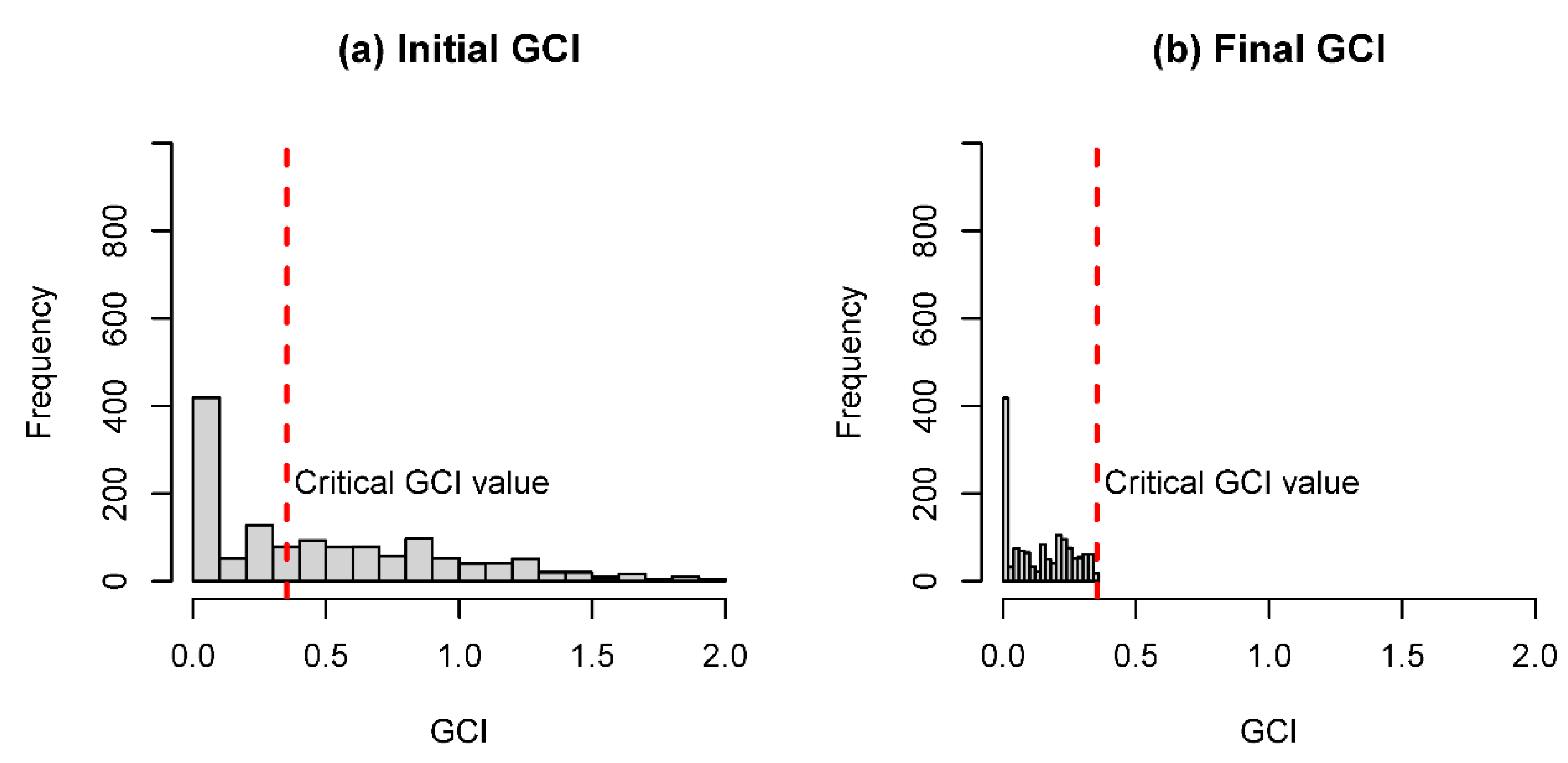
The effect of the iterative approach on the level of inconsistency for the four broad coastal attribute groups can be seen in Figure 1. The critical value in this case (i.e., n = 4) is 0.353 [43]. From the initial comparisons, only around 45% of the observations fell below the critical value. After the adjustments, all observations were below the critical value.

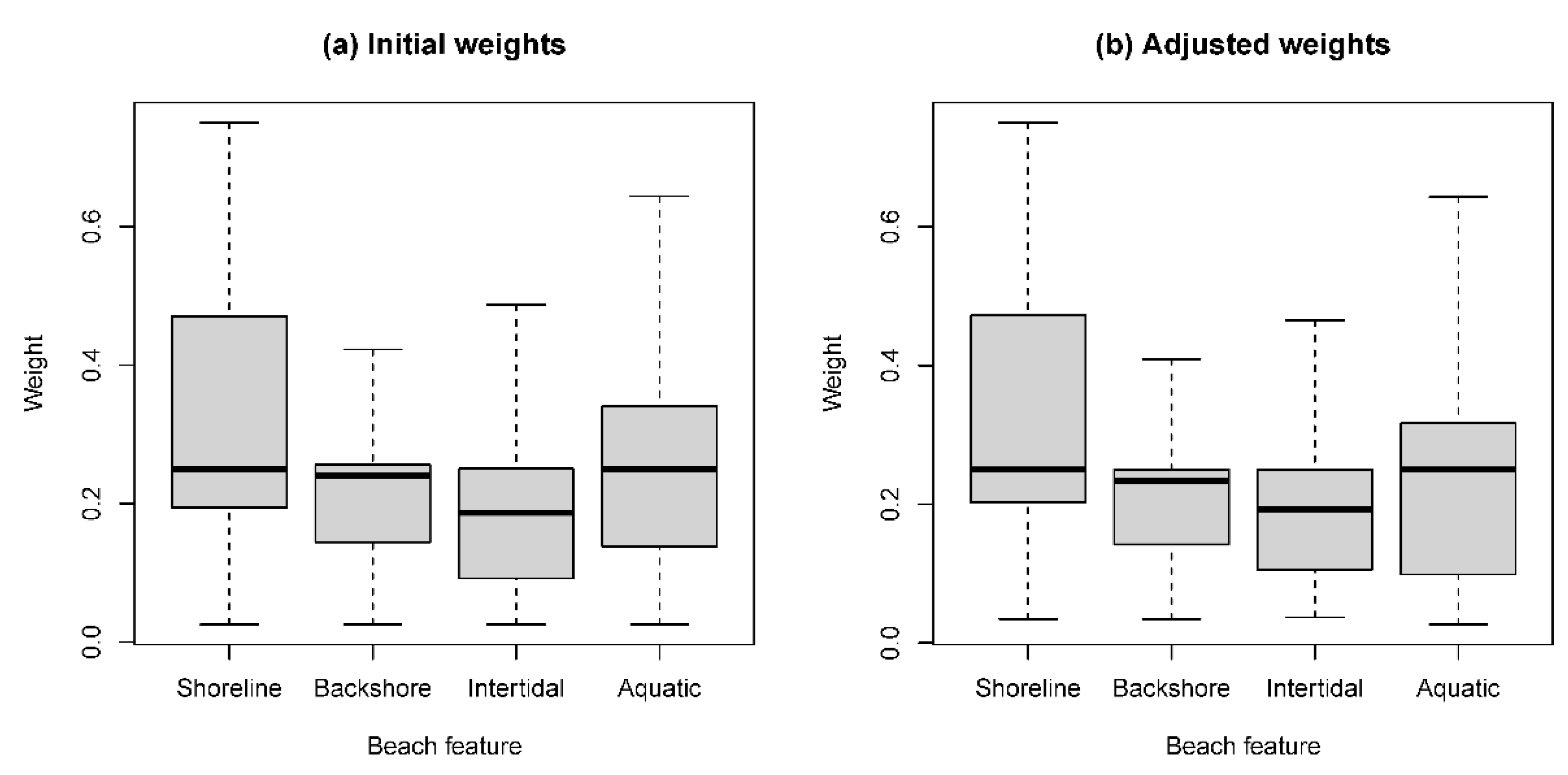
The effect of the adjustment on the distribution of the attribute weights can be seen in Figure 2 and

Table 2. Initial and revised relative weights from the example coastal case study.

	Shoreline		Backshore		Intertidal		Aquatic
	Initial	Adjusted	Initial	Adjusted	Initial	Adjusted	Initial	Adjusted
Min.	0.025	0.035	0.025	0.034	0.025	0.037	0.025	0.027
1st Quartile	0.194	0.203	0.144	0.142	0.092	0.106	0.138	0.099
Median	0.250	0.250	0.241	0.234	0.186	0.193	0.250	0.250
Mean	0.317	0.330	0.232	0.230	0.186	0.201	0.266	0.239
3rd Quartile	0.470	0.472	0.256	0.250	0.250	0.250	0.341	0.316
Max.	0.750	0.750	0.700	0.709	0.679	0.664	0.700	0.745
Correlation	0.861		0.814		0.656		0.895

, which summarizes the weights derived from all observations, including those with a GCI value above the critical value. The overall distributions varied as a result of the adjustment, but median scores were relatively constant, and the correlation between the scores before and after adjustment were high (Table 2).

The less-than-perfect correlations indicate that some scores were substantially affected. This was particularly the case for the weights associated with the intertidal coastal assets (i.e., estuaries, mangroves, saltmarshes). Respondents may have been less familiar with the ecosystem services produced by these assets compared with more familiar assets, such as beaches (shoreline) and sand dunes (backshore), and hence there may have been greater “error” in scoring these assets against others.

In terms of the ordinal ranking of the attribute weights, around 58% of the observations were unchanged, with around % changing one position (i.e., requiring two adjacent attributes to change position), and a further 14% changing two positions. The incidence of total rank reversal (i.e., changing from top to bottom and vice versa) was small, less than 0.5% (i.e., around seven of the 1414 observations). These rank changes were most likely a consequence of (non-extreme) circular triads in the data.

Approximately 25% of the respondents provided the same score for all comparisons, with 20% always choosing an equal score. Only a small proportion (0.5%) always chose an extreme score (i.e., 9 or 1/9). While the extreme cases were small, around 13% always provided a score greater than 1 for all comparisons, and 7% always provided a score less than 1. Comparing the actual score with the expected score based on the other scores, the expected direction of preference was reversed 47% of the cases for Shoreline-Backshore; 43% for cases for Shoreline-Intertidal, and 30% for Shoreline-Aquatic. Not all of these changes were necessarily implemented, but the magnitude of the potential changes demonstrates the prevalence of circular triads in the data.

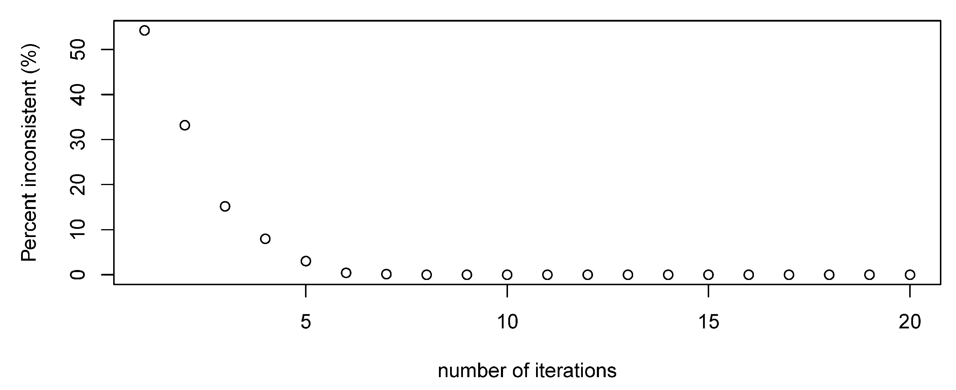
A limit on the number of iterations that could be undertaken was imposed for practical reasons, as the analysis could potentially cycle without achieving an acceptable level of consistency. While a limit of 20 iterations was (arbitrarily) imposed, the proportion of inconsistent observations decreased rapidly, with only one inconsistent observation remaining after seven iterations and none after eight (Figure 3).

4. Discussion

The automatic adjustment of inconsistent AHP matrixes is contentious, with some authors suggesting that, at best, the approaches should only be used to provide additional information to the original respondents, who should have the final say in how the matrix is to be adjusted [28,29]. While this has advantages when dealing with small groups that will be directly affected by the outcomes of the management decision making, the shift to large online surveys of a broader stakeholder group makes such individual interactions difficult, particularly if data are collected anonymously.

Several different approaches have been tried to avoid the problem of inconsistencies in online surveys. Meißner, et al. [44] suggested an adaptive algorithm to reduce the number of pairwise comparisons a respondent is faced with given their initial consistency of response, with some combinations excluded from the survey and their values subsequently estimated based on the provided responses. While this approach has attractive features, programming of such an algorithm into an online survey would be complex.

The problem of inconsistencies can also be minimized through appropriate hierarchy design. The number of comparisons required to be made by respondents increases substantially with the number of criteria to be compared: a survey with n criteria will require n(n − 1)/2 comparisons. Saaty and Ozdemir [45] suggest that the ability of respondents to be able to correct their own inconsistencies diminishes asymptotically to zero with an increasing number of criteria, with seven being an upper limit beyond which “recovery” is unlikely. With online surveys, the ability to return to respondents is limited (if not infeasible), so fewer comparisons are required to ensure inconsistencies are minimized in the first instance. The algorithm in this study is more readily applied in cases with four or less criteria being compared (after which some of the alternative approaches discussed in the earlier sections of the paper may be more suitable). Developing a hierarchy with four or less criteria in each level results in a manageable set of comparisons (i.e., 4(4 − 1)/2 = 6) and a relatively straightforward process to adjust for any inconsistencies that emerge.

Although this approach was motivated by a need to adjust inconsistencies observed in a large online survey, there are advantages also in considering the approach for smaller groups. Providing suggested modifications to the initial matrix to aid the respondents in re-assessing stated preferences to improve their consistency is often undertaken, e.g., [28,46]. However, in some cases, this can result in undesirable behavior. Recent experiences with deriving objective preference weightings in the marine and coastal environment from stakeholder groups, e.g., [14,18], have found that some stakeholders felt that, by asking them to reconsider their preferences based on their level of inconsistency, the analyst was attempting to “push” their responses to a more desired (predefined) outcome and resisted changing their answers. Some also were offended by the idea that they were considered “inconsistent” in their views and insisted on maintaining their initial stated preferences.

Even those who were prepared to change their responses exhibited undesirable behavior in some case, focusing more on trying to ensure consistency than on their actual preferences, effectively game playing to get the “best” score they could. This often resulted in these individuals moving their preferences closer to the center position in the bivariate comparisons (i.e., equal preference) to ensure a high consistency score. This satisficing response has been observed elsewhere and is a long-standing issue with attitudinal surveys [47]. Satisficing behavior particularly increases when the difficulty of the task increases (i.e., producing consistent preferences) and the respondent’s motivation decreases. Motivation in turn is affected by respondents’ belief that their responses are considered important and will contribute to a desirable social outcome [47]. In large scale surveys, individuals’ perceptions of their own impact on the outcome are likely to be low, and as a consequence care taken when completing the survey may be less than for smaller groups with a direct link to the outcome [22]. In addition, the added complexity of revising their answer to achieving a target (or maximum) level of inconsistency increases the likelihood of satisficing behavior [48]. While several online studies have included a feature which reported on the consistency of the response and provided an opportunity for a revision, e.g., [18,20], asking for revisions may not provide any more useful information than can be derived using more automated methods based on their initial preferences.

In our coastal case study, we placed a limit on the number of iterations in the algorithm. In contrast, the algorithm proposed by Cao et al. [26] repeated until acceptable levels of consistency were obtained. Similarly, the similar approach proposed by Kou et al. [36] assumed only one iteration would be sufficient, and the examples provided (including one with a circular triad) achieved consistency with one iteration. However, in the case of extreme circular triads, we found the potential for the algorithm to cycle between different potential solutions without achieving the desired consistency level. The limit chosen in the example was arbitrary. In this case, acceptable levels of consistency were obtained after one iteration for most comparisons. All values were found to be consistent within eight iterations. Alternatively, a loop function can be included that continues until all observations achieved acceptable levels of consistency, as in the work of Cao et al. [26], although for large samples, such as that used in this example, this may potentially result in a large number of iterations (and potentially an infinite loop). Given this, there are likely to be benefits still in imposing a finite number of potential iterations. There is potentially a trade-off, then, between an acceptable number of modifications/iterations and consistency levels.

Circular triads in the data were also responsible for changes in preference ranking for some respondents. Given the existence of circular triads, the original rankings were most likely spurious. A one- (or even two-) position change may be reasonable in such a case. However, without actual verification with the respondent, there is no absolute guarantee that the revised ranking is more appropriate than the initial ranking. Nevertheless, the revised ranking is based on scores that, themselves, have been based on the full set of information available, and are hence likely to be more reliable than the known unreliable scores. This is an area for further consideration and investigation.

5. Conclusions

The aim of this paper was to present a simplified approach to adjusting AHP stated preferences ex post to reduce the level of inconsistency in the results. Unlike many previous proposed approaches to adjust the comparison matrix, we ignore the initial relative weights and the eigenvector (which is not calculated when using GMM to derive weights). Instead, we examine the initial stated preferences in the original pairwise comparison matrix and identify which of these is most inconsistent given the other stated preferences. This approach is largely consistent with the original analysis of Finan and Hurley [25]. who found that improving the consistency of the final pairwise comparison matrix is likely to enhance the reliability of the AHP analysis. The approach is well suited for analyses of online survey responses, when interacting with the respondent is impractical, or may introduce other biases into the analysis.

The approach developed in this study was developed primarily for analyses of large sample online survey responses, when the potential for many inconsistencies is high (i.e., due to the large number of respondents) and interacting with the respondent is impractical or may introduce other biases into the analysis. In contrast, most other previous approaches to correct for inconsistencies were largely applied to relatively small groups of respondents. Appling these other approaches at a larger scale, while possible, is likely to be impractical.

While we have demonstrated that correcting inconsistences in such surveys is possible, this does not mean that survey design is not important. The potential for inconsistencies in online AHP surveys can be minimized through appropriate hierarchy design (i.e., avoiding large comparison sets), and this should be undertaken as a first step, with ex-post correction seen as a fallback activity.