1. Introduction
In this paper, we develop a mathematical model of the filtration flow of a liquid in a piecewise homogeneous porous medium and apply it to the simulation of lymph flow in a lymph node.
The classical model of filtration flow relies on Darcy’s law, which is valid in a linear porous medium. The numerical methods for solving problems of natural convection in porous media go back to the work of Chan et al. [
1], where the finite difference method (FDM) was applied. Hickox and Gartling [
2,
3] used the finite element method (FEM), and Prasad and Kulacki [
4] applied the finite volume method (FVM). The finite element and finite volume methods have been widely developed for solving various problems, including those in complex inhomogeneous regions (see, for example, [
5,
6,
7,
8]).
The traditional application of the filtration flows models is to the problem of fluid flow in different soils. The typical examples are the water intake problem and the oil flow to oil wells. On the other hand, modeling the fluid convection in living organisms and, in particular, the modeling of the lymph flow has its own specifics. There are just a few works that have considered the lymph flow in the lymph node by means of direct numerical simulations. The fluid flow description by Darcy’s law in inhomogeneous regions (hydraulic conductivity is not constant) is due to Rose et al. [
9]. In Moore et al. [
10], a filtration domain was piecewise homogeneous, and the filtration flow was viscous, described by the Darcy–Brinkman law. The absorption of lymph into the blood in both papers was characterized by Starling’s law, which relates the divergence of the velocity field to the fluid pressure. In all these models, the FEM approach was used.
If the domain consists of several homogeneous subdomains, then the boundary integral equations method is preferable, and the main goal of this work is to apply this method to the lymph filtration problem. In fact, this method is effective if an integral representation for a solution over domain and subdomains boundaries exists. If the latter is true, then the approach has a number of advantages over the finite difference and finite element methods applied directly in the spatial domain. First, the dimension of the problem being solved is actually reduced. Two-dimensional integral equations (two-dimensional grids) are used instead of three-dimensional grids. Moreover, the differential equations outside the boundary surfaces and conservation laws for the numerical solutions are fulfilled. Finally, the integral representations of unknown functions allow us to calculate derivatives and various functionals without a significant loss of accuracy compared to the accuracy of numerical approximation of the functions themselves.
We can single out a number of papers in which the boundary element method was applied to the modeling of flows in porous media governed by Darcy’s law or the Darcy–Brinkman law [
11]. The solution of a viscous fluid filtration problem governed by the Darcy–Brinkman law using the boundary elements method (BEM) was constructed in [
12,
13]. However, these papers only considered two-dimensional problems in a homogeneous domain with the boundary condition set only on the outer boundary. The method of fundamental solutions (MFS) was presented in [
14,
15,
16] for two-dimensional problems. This method was similar to the boundary element method, except that the solution was a superposition of partial solutions, the functions of source points located outside the flow area. That allowed avoiding singularity in the boundary condition. In this case, the method of boundary integral equations was applied to flows in one homogeneous region.
The application of the boundary integral equations method to the filtration problems in piecewise homogeneous domains was developed in the works of Piven et al., where two-dimensional flows were studied. A systematic presentation of these results can be found in [
17]. A three-dimensional model of the fluid filtration was developed by Lifanov et al. [
18]. The authors considered the filtration flows in a piecewise homogeneous domain with different types of external and internal boundaries and with the conjugation conditions at the interfaces between media with different properties. However, in all these works the flows with viscosity and absorption were not considered. The latter is important for the correct modeling of lymph flows in a lymph node.
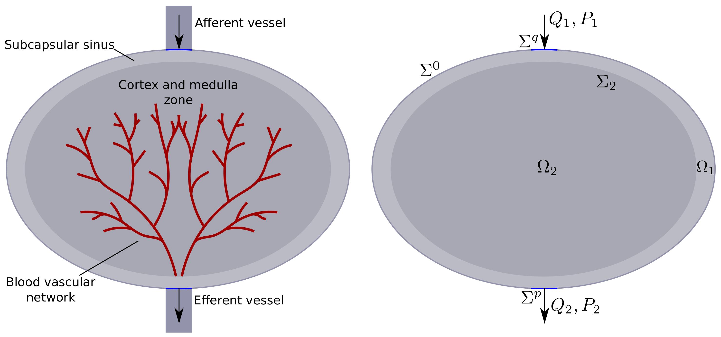
In this paper, we use a simplified lymph node model consisting of two homogeneous domains: the outer one is the subcapsular sinus, the inner one is the T-cell and medullary zones. The inner region is characterized by a significantly higher hydraulic resistance and the presence of blood vessels absorbing lymph [
19,
20,
21,
22]. In the lymph nodes, the lymphatic and circulatory systems are conjugated. The overall fluid balance in the lymph node is determined by the pressure field, permeability, and location of blood vessels, in particular, high endothelial venules [
20,
22]. The structure of the lymph node is shown schematically in
Figure 1.
In the previous works of the authors [
23,
24], a solution to the problem of fluid filtration in a piecewise homogeneous porous medium governed by the Darcy–Brinkman law was developed. In [
23], we implemented the reduction in the boundary value problem in partial derivatives to a system of boundary integral equations and also proved the equivalence of the boundary value problem and a system of boundary integral equations. In [
24], we constructed and verified a numerical scheme for solving a system of boundary integral equations with piecewise constant approximations and collocations.
In this paper, we consider the problem of a stationary three-dimensional filtration flow with absorption in a piecewise homogeneous medium. The filtration is described by Darcy’s law, and the absorption is described by Starling’s law. A characteristic feature of such a flow is a nonzero divergence. We propose an integral representation for the velocity and pressure fields of the filtration flow. We also develop numerical schemes and verify the numerical results by comparison with experimental data of the filtration in the lymph node.
2. Mathematical Model
We denote
the filtration domain, bounded on the outside by a closed smooth surface
.
–boundary between the more permeable external subdomain
and the less permeable internal subdomain
. An example of the computational domain is shown in
Figure 1 (on the right).
Fluid filtration in both subdomains is described by Darcy’s law for unknown fields of velocity
and pressure
p. In the external subdomain, the velocity satisfies the continuity equation. In the internal subdomain, Starling’s law describes the absorption of fluid in capillaries. This model is similar to one given in paper [
9]. Thus, the filtration–absorption problem can be written as a system of partial differential equations (
1).
The model parameters are —the coefficients of hydraulic conductivity in subdomains , , —the lymph dynamic viscosity, —the blood vessels’ absorption coefficient, A—the surface area of the blood vessels, —the blood pressure, —the mean difference in the oncotic pressure of blood and lymph, and —the oncotic reflectance.
The outer boundary is divided into three parts: the openings of the afferent (inlet) vessels with the given lymph inflow (), the openings of the efferent (output) vessels with the given pressure (), and the impenetrable outer border with zero lymph flow (). . The inner boundary is homogeneous. The pressure and the normal component of the velocity vector must be continuous on this boundary.
We assume that each of the surfaces
,
is oriented so that the outer side is considered positive. Let
,
,
, be the unit vector of the outer (positive) normal to the surface
at the point
x. The following boundary conditions are set on the boundaries of the domains:
Here, is the known lymph flux, . is the known pressure on . An additional variable is introduced into the system of boundary conditions: is the unknown lymph flux on the surface , .
For simplicity, we introduce the notation:
We exclude the variable
from the system (
1) by applying the
operator to the first equation of system (
1) and substituting the second and third equations.
The pressure in the external subdomain
satisfies the Laplace equation.
In the internal subdomain
, the pressure satisfies the Helmholtz equation:
If , then .
2.1. Simple and Double Layer Potentials
The particular solutions of the Laplace and Helmholtz equations in the domain are the potentials of a simple and double layer on the boundary of the domain. The simple layer potential for the Helmholtz equation placed on the surface
is the function
with
, and
h is the density of a simple layer potential, which is a function given on the surface
.
If
, then the simple layer potential
is defined by Formula (
8) even for
(see [
25]).
Moreover, under certain smoothness conditions of the density
, the following formula is valid for the boundary values of the gradient of the simple layer potential [
25]:
where
is the so-called direct value of the gradient of a simple layer potential, determined by the formula
where the integral is considered in the sense of a principal value.
The double layer potential for the Helmholtz equation
with density
g set on the surface
is the following integral operator:
The double layer potential with density
, defined by Expression (
11) at the points of the space
, is a harmonic function on this set. The double layer potential can be extended on the surface
from the external and internal domains
and
(see [
25]). The boundary values of the function
on the surface
are given by the expression:
with
being the direct value of the double layer potential obtained directly from Expression (
11) at point
.
If the double layer potential density
satisfies a certain smoothness condition, then the vector field
can be continued onto the surface
from each of the domains
and
. For the boundary values of the gradient of the function
, the formula is valid [
25]:
The direct value of the double layer potential’s gradient at the boundary of a closed surface is the following expression:
The simple or double layer potential for the Laplace equation is a particular case of the Helmholtz potential with .
2.2. Boundary Integral Equations
Following the reasoning given in [
23], we put a simple layer potential on the outer surface
and a simple layer and double layer potentials on the inner boundary
. Thus, the field of velocities and pressures in the regions
,
are sought in the following form:
Here,
in
,
in
, and
is the domain indicator function for
. The advantage of this representation is that the velocity and pressures are expressed by the same operators in different domains.
The velocity and pressure in the integral representations (
15) and (
16) satisfy system (
1). The integral representations (
15) and (
16) are substituted into the boundary conditions (
2)–(
5). We construct a system of integral equations for the unknown densities of the simple and double layer potentials
h,
g in which each equation corresponds to one of the boundary conditions (
2)–(
5).
The solution functions
h,
g of the boundary integral equation system allow calculation of the velocity and pressure fields in integral form (
15) and (
16) in the filtration domain
.
3. Numerical Method
We use the method of piecewise constant approximations and collocations for the numerical solution of the system of integral equations. This method has a low order of accuracy, but it also has such advantages as versatility, simplicity of implementation, and reliability. This is why the method is convenient for conducting computational experiments to test new mathematical models.
The surfaces
,
, are approximated by a system of triangular and rectangular cells with all the cells’ vertices lying on the surface being approximated.
Each cell has its local basis consisting of a normal vector
and two tangential vectors
,
. We also set a collocation point
on each cell
,
. The example of surface approximation is given in papers [
24,
26].
We approximate unknown functions
by piecewise constant functions
set on the approximate surfaces
,
. We set
for function
h, and
for function
. These qualities are satisfied at the internal points of the cells. The
is the cell edge.
3.1. Approximation of the Integral Operators
Let
S be one of the surfaces
,
, and
is its approximation. We approximate the direct values of the integral operators
,
,
in collocation points
,
, and the following formulas:
Here, , and m is the number of subdomains where the direct value of the potentials are calculated. Note that if , the integrals are improper absolutely convergent, and , are singular considered as the principal value.
The direct values of the double layer potential gradient
in collocation points
are approximated the following way:
To calulate the integral
, we separate the singularity and integrate it analytically. We decompose the function
into
with
. So, the integral is decomposed the following way:
To caluclate
, we use the Biot–Savart law [
27,
28], and integral
is improper convergent.
The integrals in expressions
,
,
, and
are calculated approximately by the rectangular method. Such a scheme for improper and singular integrals was described in the paper [
24].
3.2. Approximation of the Boundary Equations
To calculate the approximate solution, we use the collocation method. Equations (
17)–(
20) must be fulfilled at collocation points
,
.
After solving the system of linear Equations (
22)–(
25), we calculate the velocity and pressure fields in point
,
by the approximations of Formulas (
15) and (
16):
with
. The integrals in the expressions
,
,
, and
are proper in the inner points of the domains
,
. These integrals are also calculated by the rectangle method.
4. Results
The papers [
29,
30,
31] contained the measurements of the lymph flow, pressure, and protein concentration in the popliteal lymph nodes of dogs. To verify the model, we used the experimental data given in these papers. We constructed a geometrical model approximating the lymph node and set the boundary conditions according to the experimental data. Then, we solved the parametrical optimization problem to fit the experiment.
The fluid exchange between the lymph node and the circulatory system is described by Starling’s law (
1), the third equation. The value of parameter
was set at 0.88, according to [
10]. The experimental data presented in [
31] contained the blood pressure
and the protein concentration in the blood
and the lymph
. The oncotic pressure was calculated by the formula
, with
kg/mol as the molar mass of proteins,
as the universal gas constant, and
K as the absolute temperature. Given these data, we calculated
.
The experiment was carried out on the lymph node with one inlet opening
with a fixed flow
and one outlet opening
with fixed pressure
(see
Figure 1 on the right). The external subdomain
was ellipsoid with radii
mm, and
mm. The internal subdomain
was ellipsoid with radii
mm, and
mm. The afferent and efferent lymphatic vessels were considered to be cylindrical with the radius
mm and the centers
and
located on the upper and bottom poles of
, respectively.
The surfaces
and
were approximated as follows:
We approximated the velocity functions
and
on the parts of the boundary
and
, so that the flow through the openings had a parabolic profile. The pressure on the outlet was assumed to be constant.
The function on part of surface was approximated in a similar way.
The known experiment did not contain the complete description of all the parameters that arise in the mathematical formulation of the problem, since it is extremely difficult to calculate such measurements. Therefore we used the following approach: part of the experimental data were used as the initial parameters of model, and the other part of the data were used for validation of the model. We denoted the model parameters
. We approximated the boundary integral Equations (
17)–(
20) by a numerical scheme (
22)–(
25) and solved the corresponding linear system with parameters
and boundary conditions (
28) with the values
and
taken from paper [
31] (
Table 1).
To compare the mathematical model prediction with the experimental data values of the outlet flow
and inlet pressure
, we calculated the pressure
on
and the flow
on
using the following formulas:
The article [
31] provided data on several animals (greyhound dogs) with a number of experimental values for each animal. Assuming that different animals corresponded to different values of the
parameters, we calculated the optimal values of the parameters that minimized the functional
for all experiments for each animal.
Here, and were the i-th experiment data values, and and were calculated by the numerical model for the i-th experiment boundary condition values. To solve the optimization problem, we used the Nelder–Mead method.
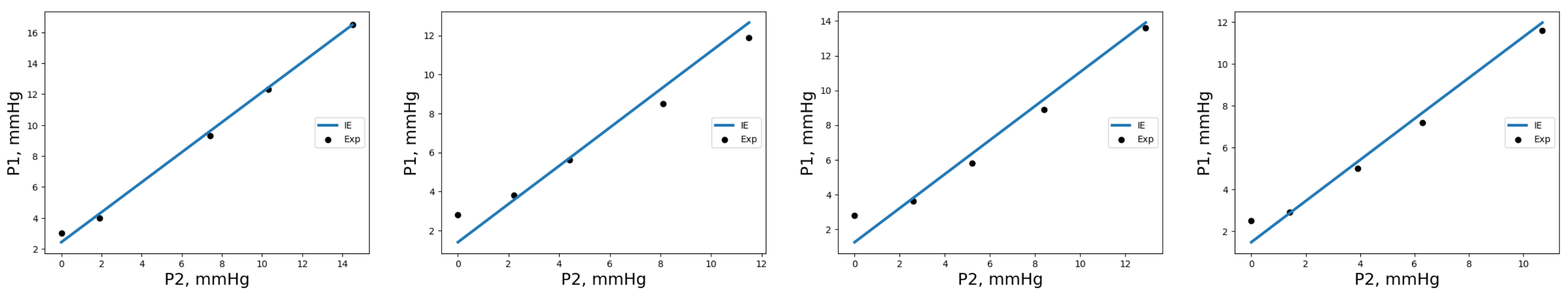
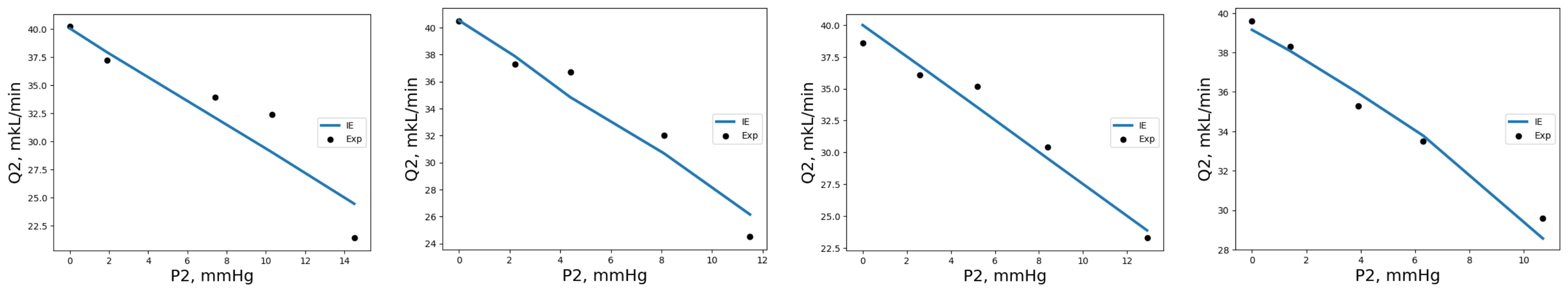
The values of the functional as well as the optimal values of the parameters are given in
Table 1. In the experiment, the value of
varied, while
had a small variation, and
was constant. So, the comparison of the simulation results with the experimental data can be represented as the dependence of
and
on
(see
Figure 2 and
Figure 3).
The value of the deviation of the results from the experiment demonstrates that the model accurately approximated the data for four animals.
5. Discussion
In this paper, we proposed a model of the fluid filtration flow in a piecewise homogeneous domain containing porous medium and applied it to the simulation of the lymph flow in the lymph node. We also assumed that the fluid was absorbed in the inner subdomain. A mixed boundary condition was set on the outer boundary of the domain (the pressure was set on the outlet opening, the flow was set on the inlet opening, and the impermeability condition was set on the remaining part of the boundary). At the interface between the media, the conjugation conditions were set (the continuity of the pressure and the normal component of the fluid velocity). An integral representation of the velocity and pressure fields in terms of the potentials of a simple layer and double layer at the domain boundary was proposed. The boundary value problem was reduced to a system of boundary integral equations for unknown densities of simple layer and double layer potentials.
A numerical solution scheme based on the method of piecewise constant approximations and collocations was constructed for the system of integral equations. The solution of the approximated system of boundary integral equations allowed calculation of the velocity and pressure fields in any inner point of the domain.
The model predictions were also compared with the existing experimental data on lymph filtration in the lymph node. An agreement between the values of the total flow characteristics obtained by numerical simulation and the experimental data was reached. The analysis of the obtained test results, in particular, showed the applicability of the developed numerical model for the simulation of the considered class of filtration flows.
The results of this work were used for the development of an artificial neural network model describing the lymph node drainage function, which was described in [
32].


