1. Introduction
In industrial applications, developing efficient numerical methods to solve the underlying partial differential equations (PDEs) requires simulations in higher dimensions and large computational domains. Such domains often consist of subdomains with different geometrical shapes and material properties. In this regard, domain decomposition (DD) methods, leading to efficient schemes, have gained considerable interest in the numerical analysis community, see [
1,
2]. A certain variant of the DD method, described below, is the subject of our current research on Maxwell’s equations, which is closely related to the schemes that were previously studied in [
3,
4]. More specifically, the present work is a further development of the DD hybrid finite element/finite difference (FE/FD) method for time-dependent Maxwell’s equations for an electric field in non-conductive media.
A stable, time-domain (TD), DD scheme for Maxwell’s equations was proposed in [
5,
6] and further verified in [
7]. This method uses the Yee scheme [
8] on the structured FD part of the mesh, and finite elements, possessing edge elements, on the unstructured part. Because of the presence of edge elements, implementing this method remains computationally expensive. A domain decomposition FE/FD method for time-dependent Maxwell’s equations for an electric field, assuming constant dielectric permittivity function in finite difference domain, was considered in [
3]. The constant permittivity assumption simplifies the numerical schemes in both FE and FD domains and significantly reduces computational efforts to implement the considered DD scheme. A modified numerical scheme, energy estimate, and numerical verification of this method were presented in [
4]. However, stability and convergence analysis with numerical implementations, in
- and
-norms of the developed FE/FD schemes, are not presented in the above studies. This work is meant to fill the gap.
More specifically, we present stability analyses for explicit schemes for FE (stability of FD is as in [
5,
6]), in the DD hybrid FE/FD method. The domain decomposition method (DDM) is constructed such that
FEM and
FDM coincide on the common, structured, overlapping layer between the two subdomains. The resulting domain decomposition approach at the overlapping layers can be viewed as a FE scheme which avoids instabilities at the interfaces. We decompose the computational domain such that
FEM and
FDM are used in different subdomains:
FDM in simple geometry and
FEM in the subdomain where more detailed information is needed about the structure of this subdomain. This allows the application of adaptive
FEM in such subdomain, see, e.g., [
3,
9], and the references therein.
Reliability and convergence of the domain decomposition method studied in this work are evident for the solution of coefficient inverse problems (CIPs) in
, see, e.g., [
9], and the references therein. For the case of CIPs, the computational domain is split into subdomains such that a simple discretization scheme can be used in a large region and more refined discretization scheme is applied in smaller, but more critical, parts of the domain. In most algorithms for solution of electromagnetic CIPs, to determine the dielectric permittivity function inside a computational domain, a qualitative collection of experimental measurements at the boundary or in a neighborhood of it is necessary. In such cases, it is convenient to consider the numerical solution for Maxwell’s equations in different subdomains with a constant dielectric permittivity function in some, adequately chosen ones, and non-constant in other ones. For time-dependent Maxwell’s equations, the DD scheme of [
4], analyzed in the present work, is used for the solution of different CIPs in order to determine the dielectric permittivity function in non-conductive media using simulated experimental data.
There are many other studies relevant to this work, e.g., in [
10,
11,
12,
13,
14,
15] and references therein. However, our analysis of DDM significantly differs from these works. In addition to optimal convergence of the constructed scheme, the novelty and scientific impact of the paper is in tackling coercivity (or lack of coercivity). More specifically, a challenging issue here is the lack of coercivity for the bilinear form in the presence of the time-derivative term. To circumvent this, a common approach is to split the bilinear form, separating the time-derivative term, and deriving the coercivity for the remaining sub-bilinear form. Then one may derive the convergence of the entire scheme with a time-derivative term.
An outline of this paper is as follows. In
Section 2 and
Section 3 we introduce the mathematical model, and briefly present the structure of domain decomposition FE/FD schemes and communication between the two schemes. In
Section 4, we describe the domain decomposition FE/FD method for the numerical solution of Maxwell’s equations and set up adequate finite element and finite difference schemes.
Section 5 is devoted to the stability analysis for the original bilinear form, (with a norm involving the time derivative term). In
Section 6, we derive optimal a priori error estimates in finite element approximation for the semi-discrete (spatial discretization) problem on the entire domain, which is easily reduced to the FE subdomain, having known boundary data (the restriction of FD solution to the boundary of the FE subdomain). Finally, in our conclusion,
Section 7, we present numerical implementations that justify the theoretical investigations in the paper.
2. The Mathematical Model
The Cauchy problem for the electric field
,
,
, of Maxwell’s equations, under the assumptions that the dimensionless relative magnetic permeability of the medium is
, and the electric volume charges are zero, is given by
where
and
are the dimensionless relative dielectric permittivity and electric conductivity functions, respectively.
and
are the permittivity and permeability of the free space, respectively, and
is the speed of light in free space. In this paper we consider problem (
1) in non-conductive media, i.e.,
, and hence, to begin with, we shall consider the following initial value problem
To solve problem (
2) numerically, we need to consider it in a bounded domain
, with boundary
, and employ a split scheme on
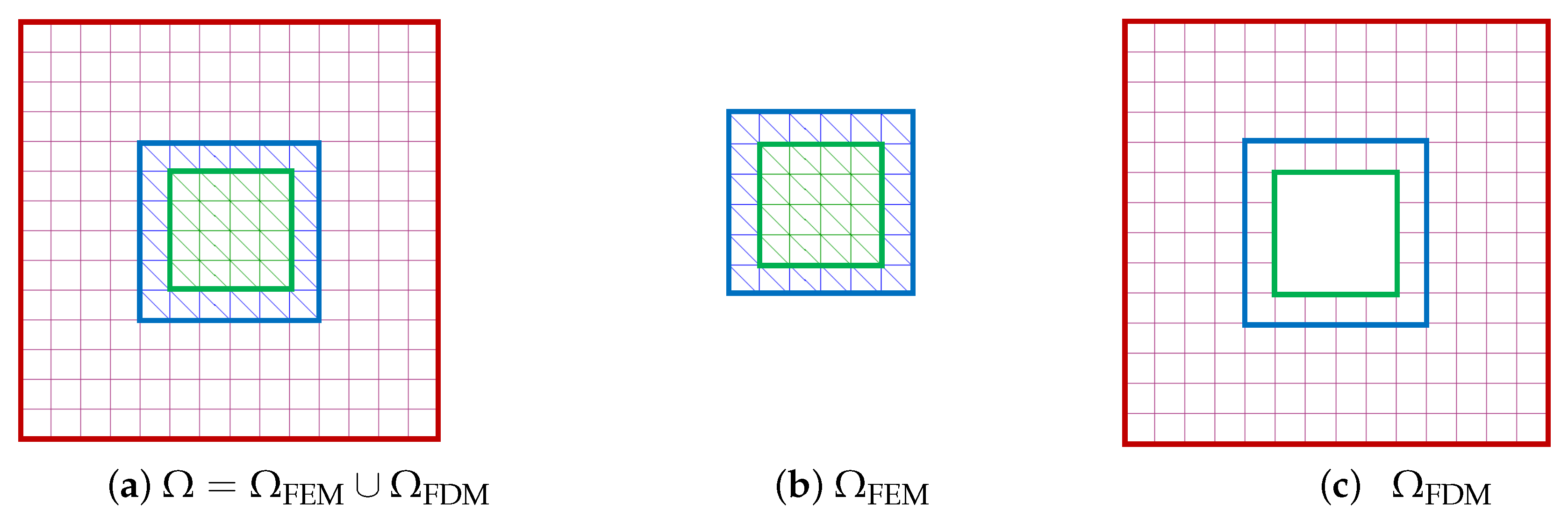
: a hybrid, finite element/finite difference scheme, a kind of domain decomposition described in Algorithm 1. In this approach, we divide the computational domain
into two subdomains,
and
such that
(note that
), and
is a subset of the convex hull of
. The function
is assumed to be constant in
, and bounded and smooth in
. The communication between
and
is arranged using an overlapping mesh structure through a two-element thick layer around
, as shown by the blue and green common boundaries in
Figure 1. The blue boundary is the boundary of
, the green boundary is the inner boundary of
, and the red boundary is the outer boundary of
(which is also the boundary of the original domain
).
| Algorithm 1 Domain decomposition process for the hybrid FE/FD scheme |
- 1:
On the mesh , where FDM is used, update the Finite Difference (FD) solution. - 2:
On the mesh , where FEM is used, update the finite element (FE) solution. - 3:
Copy the FE solution obtained at nodes (nodes on the green boundary of Figure 1) as a boundary condition on the inner boundary for the FD solution in . - 4:
Copy the FD solution obtained at nodes (nodes on the blue boundary of Figure 1) as a boundary condition for the FE solution on of . - 5:
Apply boundary condition at at the red boundary of .
|
The key idea with such a decomposition is that it allows applying different numerical methods in different computational domains. For the numerical solution of (
2) in
, we use the finite difference method on a structured mesh. In
, we use finite elements on a sequence of unstructured meshes
, with elements
K consisting of triangles in
and tetrahedron’s in
, both satisfying the minimal angle condition. This approach combines the flexibility of the finite element and the efficiency of the finite difference in terms of speed and memory usage and fits well for the reconstruction algorithm presented below.
Assumption 1.We assume that for some known constant , the function satisfies
As an immediate consequence of this assumption we have that
Assumption 1 has a physical meaning. The model problem (
2) has a lot of applications in the field of coefficient inverse problems what we have pointed out in the introduction. One of the application of the model problem (
2) is determination of dielectric permittivity function from measurements of the electric field at the boundary of the investigated domain, and this is a typical CIP. We refer for applications of such CIPs in [
9,
16,
17,
18,
19] and references therein. This CIP is an ill-posed problem and needs several assumptions in order to be able to solve it, see details in [
20,
21,
22]. One of the assumptions is the introduction of the set of admissible parameters for the dielectric permittivity function, which we define in the Condition (
3). The lower bound in this set corresponds to the homogeneous media and the upper bound
d is chosen as maximal values of the dielectric permittivity function and depends on the concrete physical problem. We refer to [
16,
18,
23,
24] where one can find values of dielectric permittivity function for different real-life applications with applications in medical imaging. Using these values can determine the upper and lower bounds in the set of admissible parameters for this function. See works [
9,
17,
19] for examples of such sets for some real physical problems.
Note further that
. Condition (
3) on
and the relation
together with divergence-free field
E, make the equations in (
2) independent of each other in
and
so that, in
(with
), we just need to solve the system of wave equations:
Remark 1. There are different discretizations of Maxwell’s equations in the time domain such as the FDTD Yee scheme [8,25], FE Lee–Madsen scheme [26], node-based least squares FE schemes [27,28], edge elements [29,30], and a number of discontinuous Galerkin FE schemes [31,32,33,34,35]. It is well known that, for stable implementation of the finite element solution of Maxwell’s equations, divergence-free edge elements are the most satisfactory ones from a theoretical point of view [29,30,36]. However, the edge elements are less attractive for the solution of time-dependent problems, since a linear system of equations should be solved at each time iteration step. On the contrary, P1 elements can be efficiently used in a fully explicit finite element scheme with lumped mass matrix, see, e.g., [37,38,39]. It is also well known that the numerical solution of Maxwell’s equations using nodal finite elements is often unstable and results in spurious oscillatory solutions [40,41]. There are a number of techniques to overcome such instabilities, see, e.g., [27,28,41,42,43]. In [
44], a finite element analysis shows stability and consistency of the stabilized finite element method for the solution of (
1) with
. In the current study we show stability and convergence for the combined
FEM/
FDM scheme, under the condition (
3) on
(the convergence would require an additional condition on
: namely (
4)) where the stabilized
FEM is used for the numerical solution of (
2) in
and the usual
FDM discretization of (
6) is applied in
.
We shall consider the following boundary and initial conditions:
Recall that we assumed non-conductive media: . In the presence of electric conductivity, additional -terms appear in the equations. Then the -term adds an analytically advantageous, parabolic character to the equation.
Hence, in this note, we assume (
3) and study the following stabilized version of the initial boundary value problem (
2), with sufficiently smooth initial data
and
:
4. Derivation of Computational Schemes
In this section, we construct a combined, finite element/finite difference scheme to solve the model problem (
8). In this approach, first, we present the finite element scheme to solve (
8) in entire
. This induces the finite element scheme in
. Then, we derive the finite difference scheme in
, when the domain decomposition FE/FD structure is applied to solve (
8) in
.
In what follows, C will be a generic constant independent of all parameters, unless otherwise specifically specified, and not necessarily the same at each occurrence.
Remark 2. The computational schemes derived in this section are explicit and therefore, for their convergence, the CFL condition below (see, e.g., [44]) should hold Here C is a mesh independent constant, τ is the time step, and h is the mesh size.
In the sequel, we denote the inner product of by , and the corresponding -norm by . The scalar inner product in we denote by , and its associated -norm by . Further, we let be the boundary of , the inner boundary of , the outer boundary of , and denotes scalar product at the boundary .
4.1. Finite Element Discretization in
First, we derive the finite element scheme to solve the model problem (
8) in whole
. The restriction of this FE solution to the inner
is the approximation for
. Next, we discretize
in two steps: (i) the spatial discretization using a partition
of
into elements
K, where
is a mesh function defined as
, representing the local diameter of elements. We also denote by
a partition of the boundary
into boundaries
of the elements
K such that in
, two of the vertices, and in
, three of the vertices of these elements belong to
. As usual, we also assume a minimal angle condition on elements
K in
, see details in [
45]. (ii) As for temporal discretization, we let
be a uniform partition of the time interval
into
N subintervals
of length
Our implementations are for fully discrete, space-time scheme. However, temporal discretization (ii), being well-studied in the literature, is not considered in the analysis here. To formulate the finite element method for (
8) in
, we introduce the finite element space
for each component of the electric field
E defined by
where
denote the set of piecewise-linear functions on
K. Setting
, and because of the homogeneous Dirichlet boundary data in (
8) we need to choose the test function space as
Then, recalling (
5) and the Dirichlet boundary condition in (
8) the spatial semi-discrete problem in
reads:
Findsuch that,
where
and
are suitable approximations for the initial data, specified below. Further, we note that
implies
Recalling (
10), vanishing test functions at the boundary yields
(
on
yields
), and the final weak formulation for the semi-discrete problem in
is:
Findsuch that,
For the reflexive, inhomogeneous boundary condition, see the FE scheme for .
To get a fully discrete scheme for (
8) we apply time discretization to (
11). Then
, denoted by
, and the central difference scheme, for
, yields
Multiplying both sides of (
14) by
we get,
that
Rearranging terms in (
15) we get the following scheme:
Given the initial data, and ,
find such that ,
4.2. Finite Element Discretization in
To solve the model problem (
8) via the domain decomposition FE/FD method, we use the split
, see
Figure 1. Thus, in
we use
FEM to solve the equation
Here,
g corresponds to the restriction of the exact solution to
. Therefore test and trial functions are not vanishing at this boundary, hence the term corresponding to
in (
11) will appear in the weak formulation for
.
To formulate the finite element method for (
17) in
, mimicking (
11), we introduce the finite element space
for each component of the electric field
E defined by
Setting
we define
to be the usual
-projection of
g in
. Then, similar to the FE scheme for
, we get the following finite element scheme for
: Given approximate values
and
of
and
, respectively, and
, find
such that
where we set
, i.e., the restriction of the finite element solution on whole
to
, (which, here, contrary to the whole domain where
, will be non-zero).
A corresponding fully discrete problem in reads as follows:
Given
,
,
,
, and
; find
such that
,
4.3. Finite Difference Formulation
We recall now that from conditions (
3) it follows that in
the function
. This means that in
for the model problem (
2) the forward problem will be
Using standard finite difference discretization of the Equation (
20) in
we obtain the following explicit scheme for the solution of the forward problem:
In the system of equations above, is the solution at the time iteration step k at the discrete point , is the time step, and is the discrete Laplacian.
Note that (
24) is associated with the Neumann boundary condition above, where the Dirichlet boundary conditions
can be considered as well.
6. Error Estimates: Semi-Discrete (SD) Problems
In what follows, assuming certain regularity of the data set,
, and with the spectral polynomial order
p chosen as the assumed regularity degree
we can prove semi-discrete spatial error estimates of the form
Below we use a very similar argument to derive (
41) for the spatial domains
and
. To do so, we rely on an approach (see, e.g., [
46]) based on a split of the bilinear form
to a temporal term, plus a time-harmonic sub-bilinear form below denoted
.
Splitting of B. Here we extract from
B the bilinear form
, by suppressing the time-derivative term, and establish well-posedness for
a. Then we deal with the convergence of the original, time-dependent scheme of
B. Thus
Due to the homogeneous Dirichlet boundary condition, the inherited Galerkin orthogonality yields:
Now we can write the equation (
25) as Find
such that for all
,
The
consistency of
is a consequence of (
44).
We also define the norm associated to
:
which, as an immediate concern, requires the condition below
The
coercivity of
is due to vanishing boundary terms and assuming (for simplicity) that
, we use the Poincare inequality
, and the second condition in (
46) to write
where the second inequality is a consequence of reusing Poincare inequality for the term
, and we have a desired coercivity for
.
The
continuity of
is evident from the coercivity (
47) and (
46), which yields
6.1. Error Estimates: SD Problem in
We define a Ritz–Galerkin type projection
by
Then using the estimates (see [
46] for the details):
and
we can deduce that (see Lemma 5.4 in [
46],
-estimate and interpolation),
Finally, we recall the Galerkin orthogonality:
Our main result is the following theorem.
Theorem 1. Let E and be the solutions for the continuous and semi-discrete, weakly formulated, problems (25) and (13), respectively. Assume that . Then, there exists a constant C, independent of , but dependant on ε, such that for , the error is estimated as Proof. We shall prove the theorem for
. The case
is a simpler version, and
follows using classical interpolation of the Sobolev spaces, see [
47]. For
, we use a split of error via the Ritz projection:
To bound
we note that using the Galerkin orthogonality (
53),
This yields (noting that
is a function only in space)
Note that, by the definition
. Hence, integrating over
we get
Now, using the fact that
, and since (
55) holds for all
,
which inserting into (
55) and using (
52) noting that
and
we get
Summing up, we get the desired result. ☐
Remark 4. Note that the errors in initial data, and , do not appear in the above estimates. In general, and for sufficiently regular and , the initial data errors can always be dominated by other error terms in appropriate norms.
6.2. Error Estimates: SD Problem in
Here the non-vanishing boundary data causes additional asymmetry (the first one:
was tackled above), which may be symmetrized using a Nitsche-type approach of [
46]. We circumvent Nitsche invoking additional conditions on the Ritz projection at the boundary
. The variational form and the finite element formulation in
are
and
respectively. Hence, subtracting (
60) from (
59), where in (
59) we restrict
, we end up with the error equation for
, in
:
To be concise, for
, we suppress the subscript
from the inner products, and to distinguish from
, use
,
, and
for the error and the bilinear forms in
. Now we define a somewhat modified Ritz–Galerkin projection:
by
with
defined as
a, but now over
, and with the additional property of satisfying weak Neumann boundary condition that behaves like Galerkin approximation:
Note that denoting
, (
61) yields a modified Galerkin orthogonality, viz.
which can be rewritten as:
Now, we follow the procedure above (using the very similar estimates of
and
for
and
), and let
Thus recalling (
65) and (
62), we end up with
The remaining part is as in the proof of the previous theorem for the error estimates for . Thus summing up we have proved the following error estimate in :
Theorem 2. Let E and be the solutions for the continuous and semi-discrete, weakly formulated, problems (25) and (13), respectively. Further, assume that , . Then, there exists a constant C depending on ε but independent of such that for and defined as in (66); Corollary 1. Under the conditions in the theorem (2) and recalling (63) we have Proof. Using the split (
66) and (
63) we have
As an immediate consequence of (
71) we get
Further, by the trace theorem
which yields the desired result. ☐
7. Numerical Examples
In this section, we present numerical examples justifying the theoretical results of the previous two sections. For convergence tests the domain decomposition algorithm (see Algorithm 2), implemented in the software package WavES [
48], was used. We note that because of using explicit FE and FD schemes in
and
, correspondingly, we need to choose a time step
according to the CFL stability condition (
9) derived in [
44] so that the whole hybrid scheme remains stable.
| Algorithm 2 Domain decomposition algorithm for the solution of Maxwell’s equation (Equation (2)). At every time step k we performed the following operations: |
- 1:
Compute in using the explicit finite difference scheme ( 24) with known , and -values. - 2:
Compute in by using the finite element scheme ( 19) with known . - 3:
For the finite difference method in , use the values of the function at nodes (green boundary of Figure 1), which are computed using the finite element scheme ( 19), as a boundary condition at the inner boundary of . - 4:
Apply appropriate boundary condition at the outer boundary of . - 5:
For the finite element method in , use the values of the functions at nodes (blue boundary of the Figure 1), which are computed using the finite difference scheme ( 24) as a boundary condition. - 6:
Apply swap of the solutions for the computed function to be able to perform the algorithm on a new time level k.
|
Numerical tests are performed in time interval
and in the spatial dimensionless computational domain
which is split into the finite element domain
and the finite difference domain
, thus
, see
Figure 1.
The model problem in all our tests that is stated for the electric field
is as follows:
We have the functions
as the exact solution
of the model problem (
76) with the source data
which corresponds to this exact solution.
The function
in (
76) is defined as
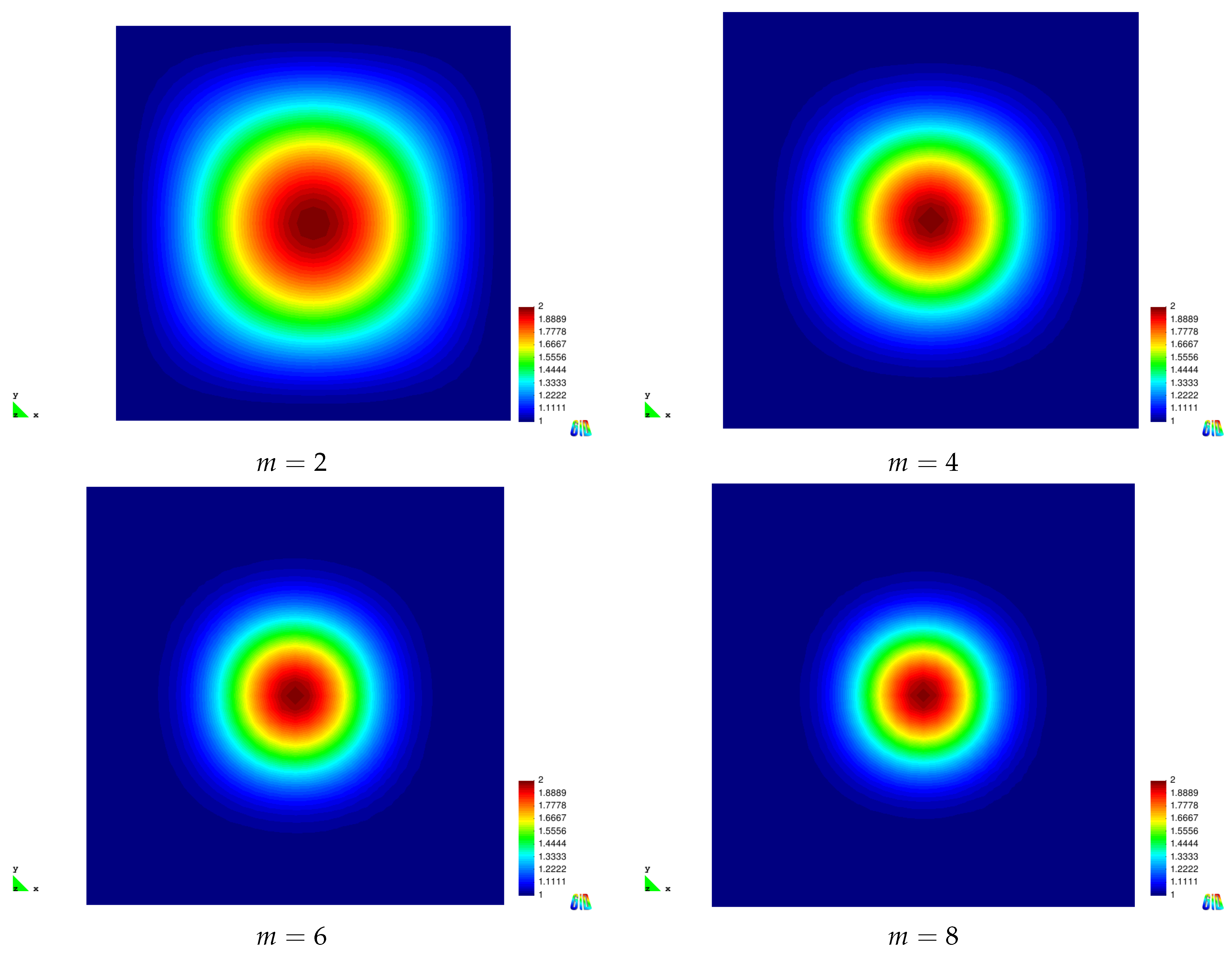
We choose
in our numerical examples, see
Figure 2, for these functions in the domain
. We note that the exact solution (
77) satisfies the divergence-free condition
for
defined by (
78), the homogeneous initial conditions, as well as the homogeneous Dirichlet conditions for all times.
The computational domain
was discretized into triangular elements with mesh sizes
, and the mesh in
was decomposed into squares of the same mesh sizes as described in
Section 3, see
Figure 1. The time step was chosen corresponding to the stability criterion (
9) as
for
. Convergence results of the proposed finite element scheme computed in
and
norms are presented in
Table 1,
Table 2,
Table 3 and
Table 4 for
in (
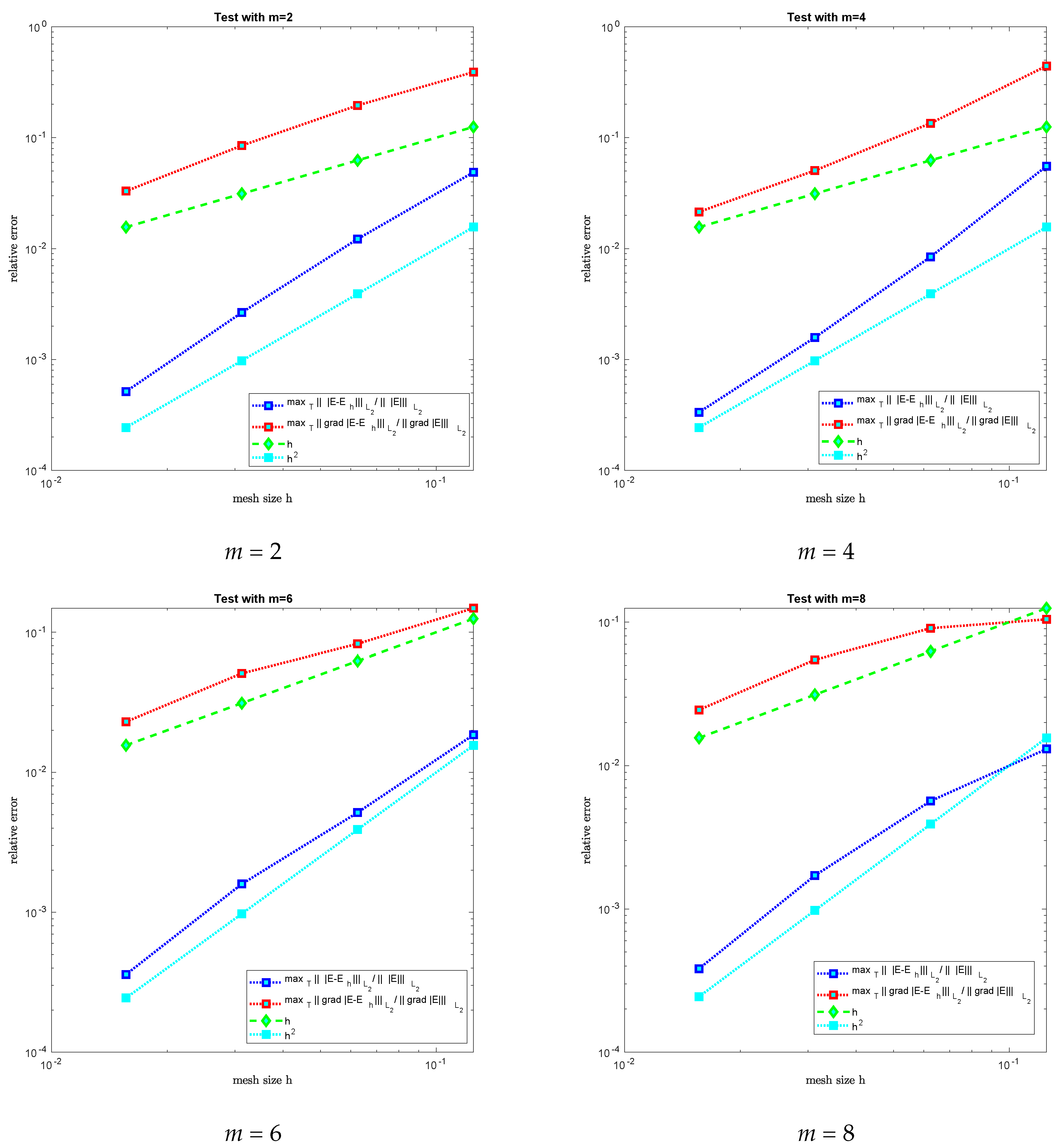
78). Relative norms in these tables were computed as
E and
are the exact and computed FE solutions in
, respectively, and
. Logarithmic convergence rates
in these tables are computed, viz.
where
are relative norms computed via (
79) on the mesh
with the mesh size
h and
, respectively.
Figure 3 shows convergence of the relative
- and
-norms computed via (
79) and compared with exact behavior of
h and
.
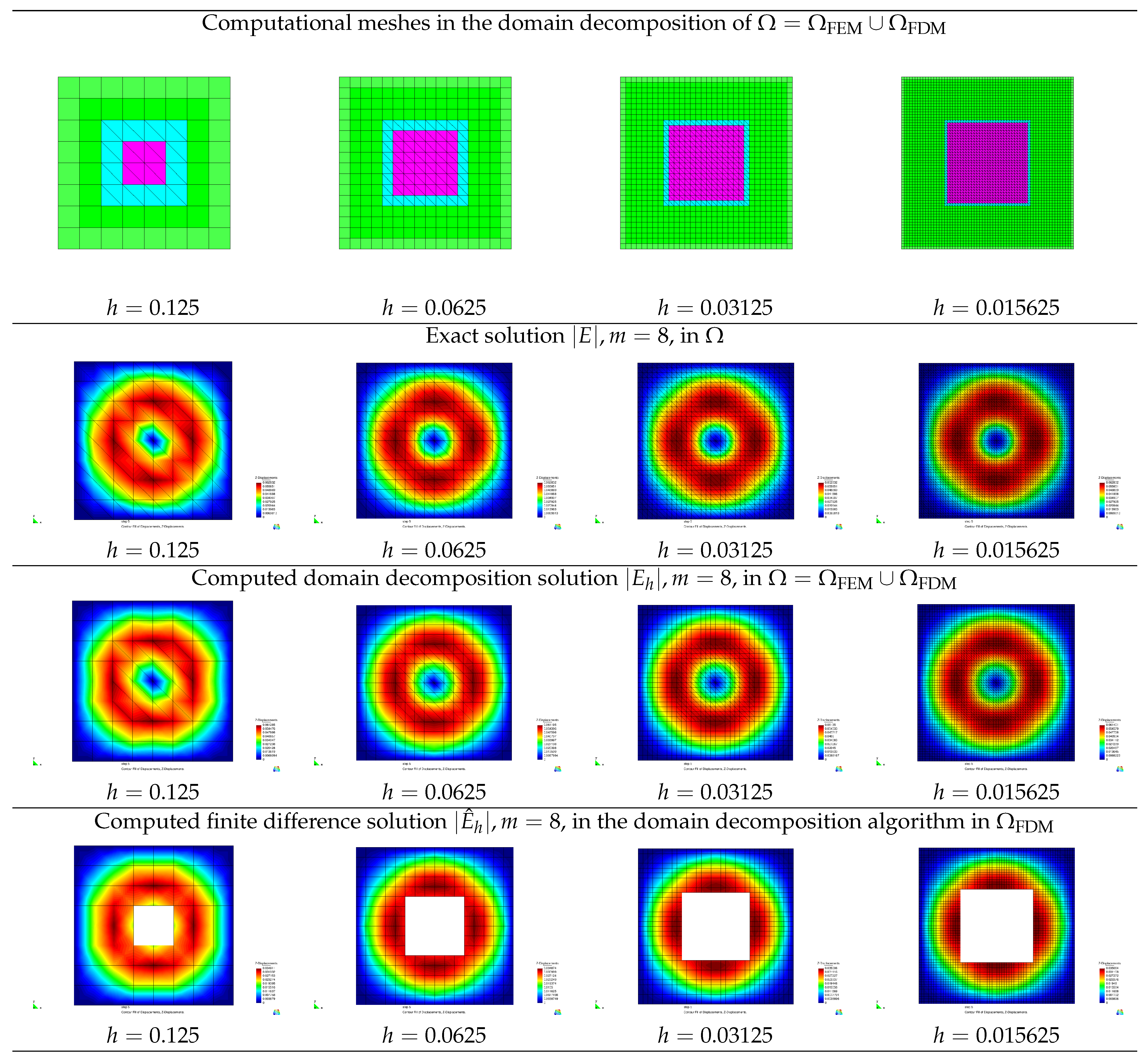
Computed hybrid FE/FD versus exact solutions with
in (
78) at the time
are presented in
Figure 4, where
is computed using the domain decomposition algorithm (Algorithm 2) for different meshes with sizes
. The top figures of
Figure 4 present hybrid FE/FD meshes which were used for computations; common hybrid FE/FD solution in
is presented in the middle figures; the bottom figures show only FD solution as part of the common hybrid solution in
. Interpreting these figures, we observe smooth behavior of the hybrid solution across finite element/finite difference boundary, as was predicted in theory.
Furthermore, through these figures, as well as tables and
Figure 3, we observe that with increasing
l in
, the computational errors approach the second order convergence in
- and first order in
-norm for
. Therefore, we can conclude that the finite element scheme in the hybrid FE/FD method, considered in
, behaves like a first-order method in the
-norm and a second-order method in the
-norm. These results are all in good agreement with the analytic estimates derived in
Section 5 and
Section 6, as well as with results presented for finite element method in [
44] for the whole
.


