Model and Training Method of the Resilient Image Classifier Considering Faults, Concept Drift, and Adversarial Attacks

Abstract

Modern trainable image recognition models are vulnerable to different types of perturbations; hence, the development of resilient intelligent algorithms for safety-critical applications remains a relevant concern to reduce the impact of perturbation on model performance. This paper proposes a model and training method for a resilient image classifier capable of efficiently functioning despite various faults, adversarial attacks, and concept drifts. The proposed model has a multi-section structure with a hierarchy of optimized class prototypes and hyperspherical class boundaries, which provides adaptive computation, perturbation absorption, and graceful degradation. The proposed training method entails the application of a complex loss function assembled from its constituent parts in a particular way depending on the result of perturbation detection and the presence of new labeled and unlabeled data. The training method implements principles of self-knowledge distillation, the compactness maximization of class distribution and the interclass gap, the compression of feature representations, and consistency regularization. Consistency regularization makes it possible to utilize both labeled and unlabeled data to obtain a robust model and implement continuous adaptation. Experiments are performed on the publicly available CIFAR-10 and CIFAR-100 datasets using model backbones based on modules ResBlocks from the ResNet50 architecture and Swin transformer blocks. It is experimentally proven that the proposed prototype-based classifier head is characterized by a higher level of robustness and adaptability in comparison with the dense layer-based classifier head. It is also shown that multi-section structure and self-knowledge distillation feature conserve resources when processing simple samples under normal conditions and increase computational costs to improve the reliability of decisions when exposed to perturbations.

1. Introduction

1.1. Motivation

Image classification is one of the most common tasks in the field of artificial intelligence. Classification analysis of visual objects is often a component of safety-critical applications, such as medical diagnostics and autopilots of public transport and combat drones. It is used in production processes, traffic flow monitoring, infrastructure inspection, industrial facilities, and other similar tasks. Therefore, there is a need to ensure the resilience of artificial intelligence algorithms, given their ability to continue to function under varying system requirements, thus changing the parameters of the physical and information environment, as well as the emergence of unspecified failures and malfunctions. In the case of artificial intelligence for image classification, specific perturbations, such as adversarial attacks or noise, faults, or fault injection attacks, as well as concept drifts and the presence of out-of-distribution samples, increase aleatoric and epistemic uncertainty, resulting in a decrease in the performance of the intellectual algorithm [1,2,3].

The resilience of the image classifier to perturbations is primarily ensured by achieving robustness in the absorption of a certain level of destructive perturbations and implementing the graceful degradation mechanism to achieve the most effective behavior in conditions of incomplete certainty [1]. Data analysis models need to be continuously improved to take into account the non-stationary environment and new challenges. This is why the ability of the model to quickly recover performance by adapting to destructive effects and improve to increase the efficiency of subsequent adaptations are equally important components of resilience [2]. Recovery and improvement mechanisms are developed within the framework of the continual learning and meta-learning frameworks [4,5].

Achieving a certain level of resilience mandates the introduction of a certain resource and functional redundancy into the system, but there are always resource constraints in practice [6]. When designing and operating resilient systems with resource constraints taken into account, the principles of affordable resilience are often used. This involves establishing an effective balance between the system’s lifecycle costs and the technical characteristics of its resilience [7]. In the case of biological intelligence, as learning progresses, the cost of decision making decreases. Mechanisms of adaptive computing and cascade or multi-branch models are concerned with achieving a biological-like performance of intelligent algorithms [8,9].

Separate components of resilience to certain types of destructive effects have been researched in many scientific papers, but the complex influence of multiple destructive factors at once has still not been considered [1,2,3]. In addition, machine learning algorithms for image classification that simultaneously implement components of resilience, such as robustness, graceful degradation, recovery, and improvement, have not yet been proposed. Not all implementations of these components are compatible, especially under resource-constrained conditions. These methodological gaps highlight the need for a research and design of image classification systems with harmonized and resource-efficient implementation of all resilience components to reduce the impact of various kinds of perturbation on classification performance.

1.2. Objectives and Contribution

The aim of the study is to develop a resilient image classifier, which would function under influence of destructive perturbations and resource constraints.

By resilient we mean a classifier, which implements the basic principles of resilience (robustness, graceful degradation, recovery, and improvement) to the selected type and level of perturbations. The less the performance of the classifier decreases under the influence of perturbation and the faster it recovers and improves, the more resilient the classifier is considered to be. Where the permissible level of performance declines and the allowable number of iterations to restore performance is known, the classifier can be considered resilient if its response to a given perturbation does not exceed the specified limits.

The key objectives are as follows:

-

To develop a new resource-efficient model and a training method, which simultaneously implement components of resilience such as robustness, graceful degradation, recovery, and improvement;

-

To test the model’s and training method’s ability to provide robustness, graceful degradation, recovery, and improvement.

Structurally, the work consists of the following sections. The related works are analyzed in the Section 2. The Section 3 presents a new classifier model used to provide resilience features. The Section 4 describes a new training method used to provide resilience features. The Section 5 describes the experimental results of testing of the proposed model and training method of the classifier. The research results are discussed in the Section 6. The Section 7 concludes the paper and describes the directions of future research.

The main contribution of the research includes a set of proposed principles, a classifier model, and a training algorithm that provides resilience capabilities to fault injections, concept drifts, and adversarial attacks. In addition, the behavior of the proposed classifier is investigated and compared with conventional approaches under the influence of the considered perturbations. The multi-section model has a hierarchical structure of class prototypes and hyperspherical class boundaries, which are optimized during training and provide perturbation absorption and graceful degradation capabilities. The novelty of the machine learning method lies in the application of a complex loss function assembled from its constituent parts in a particular way depending on the result of perturbation detection and the presence of new labeled and unlabeled data. In addition, the applied regularization provides an information bottleneck and compact distribution of classes, as well as the maximum possible interclass gaps.

2. The State-of-the-Art

Basic principles of system resilience to destructive perturbations are formulated in [6,7]. These presuppose the existence of mechanisms of perturbation absorption, perturbation detection, graceful degradation, productivity restoration, and improvement. Previous studies [1,2,3] have explored the vulnerability of artificial intelligence algorithms, identifying the following destructive effects: noise and adversarial attacks, faults and fault injection in the environment of intelligent algorithm deployment, concept drifts, and the emergence of novelty (i.e., test examples that monitor the distribution of training data).

The ability to absorb destructive perturbations is called robustness. There are many methods and approaches used to increase robustness to adversarial attacks. Some researchers separate methods for ensuring robustness to competitive attacks into the following categories: gradient masking methods, robustness optimization methods, and methods of detecting adversarial examples [10]. Gradient masking includes some input data preprocessing methods (jpeg compression, random padding and resizing [11], discrete atomic compression [12]), defensive distillation [13], randomly choosing a model from a set of models or using dropout [14], and the use of generative models (i.e., PixelDefend [15] and Defense-GAN [16]). However, [17] demonstrated the inefficiency of gradient masking methods. The robust optimization approach includes adversarial training [18] and regularization methods, which minimize the effects of small perturbations of the input (such as Jacobian regularization or L2-distance between feature representations for natural and perturbed samples) [19,20], as well as provable defenses (i.e., Reluplex algorithm [21]). The optimization approach also includes sparse coding-based methods of feature representation, which provide a low-pass filtering effect. These methods are mainly implemented on the basis of L0-regularization, L1-regularization, or similar alternatives [22]. However, robustness optimization usually requires significant computational resource consumption to obtain a good result. Finally, yet another approach lies in developing an adversarial sample detector to reject such samples at the input of the main model [23,24,25]. However, Carlini and Wagner [26] rigorously demonstrate that the properties of adversarial samples are difficult and resource-intensive to detect. The authors of [10,27,28] proposed to divide the methods of defense against adversarial attacks into two groups, implementing two separate principles: methods of increasing intra-class compactness and inter-class separation of feature vectors and methods of marginalizing or removing non-robust image features. The potential for the further development of these fundamental principles and their combination, while taking into account additional requirements and limits, is highlighted in this study [29,30].

There are three main approaches which are used to ensure robustness to the injection of faults in the computing environment where neural networks are deployed: the introduction of explicit redundancy [31,32], learning algorithm modification [33], and architecture optimization [34]. Faults are understood as accidental or intentional bit flips in memory, which store the weights or the original value of the neuron. The introduction of explicit redundancy is achieved, as a rule, via the duplication of critical neurons and synapses, the uniform distribution of synaptic weights, and the removal of unimportant weights and neurons. It is also possible to increase the robustness of the neural network to the injection of faults at the stage of machine learning by adding noise, introducing perturbations, or injecting direct faults during training [33]. The same can also be achieved by including a regularization (penalty) term in the performance measure to indirectly incorporate faults in conventional algorithms. Optimizing the architecture to increase robustness means minimizing the maximum error at the output of the neural network for a given number of inverted bits in memory where weights or results of intermediate calculations are stored. Some authors [34] solved this problem with evolutionary search algorithms or neural architecture search tools. However, architecture optimization is traditionally a very resource-intensive process.

Other papers [35,36] have proposed methods of domain randomization and adversarial domain augmentation, which increase the robustness of the model under bounded data distribution shifts. Domain randomization is the generation of synthetic data with large enough variations so that that real-world data are simply viewed as another domain variation [35]. This can include the randomization of view angles, textures, shapes, shaders, camera effects, scaling, and many other parameters. Adversarial domain augmentation creates multiple augmented domains from the source domain by leveraging adversarial training with relaxed domain discrepancy constraint based on the Wasserstein auto-encoder [36]. Transfer learning and multi-task or multiple-source domain learning also reinforce resistance to out-of-distribution perturbations [37]. However, if there is a real concept drift in the data stream, there is a need to detect such a situation and implement reactive mechanisms to adapt [38]. There are studies on adapting to the real concept drift, but the lack of labels for test data or a significant delay in obtaining them remains a challenge. One of the successful approaches in reducing data quantity requirements and increasing the generalization ability of the model involves transferring labeling information across heterogeneous domains, cross-domain information may not be available for some applications, however [39,40].

Adversarial attacks, fault injections, concept drifts, and out-of-distribution examples cannot always be absorbed, so the development of reactive resilience mechanisms, namely graceful degradation, recovery, and improvement, remains relevant [2,6]. In [41], mechanisms of nested learning and hierarchical classification are proposed, particularly useful for the implementation of the graceful degradation mechanism. However, the implementation of these mechanisms is often associated with the need to detect perturbation. The most successful methods of detecting adversarial and out-of-distribution samples and concept drifts are based on the analysis of high-level feature space using a distance-based confidence score or prototype-based classifier [25,42,43]. In [44,45], sum checking and low-collision hash function are proposed in order to detect changes in the neural network weight under the influence of memory faults. In [46], the mechanism for detecting faults affecting inference is based on the calculation of the contrastive loss function reference value on the test diagnostic samples of data in the absence of faults. To detect faults, the current value of the contrastive loss function for diagnostic data is compared with the reference value. In addition, a restoration of damaged neural network weights can be implemented by fine-tuning [46,47].

Other papers [48,49] consider algorithms for adapting models to destructive perturbations, where the principles of active learning or contrastive learning are used to speed up adaptation by reducing the requirement for labeled data in quantities. Semi-supervised learning methods are proposed in [50] for the simultaneous use of both labeled and unlabeled data in order to accelerate adaptation to the concept drift. The methods of lifelong learning, which help to continuously accumulate and improve knowledge from different tasks, as well as different reminder mechanisms, which help to avoid catastrophic forgetting problems, are considered in [5,51]. Various approaches to the implementation of meta-learning to improve the effectiveness of adaptation are covered in [4,51]. In addition to improving the model performance, [52] considers the principle of self-distillation for training neural networks, which can implement adaptive calculations and speed up the inference mode as the learning efficiency of the lower layers. This property of inference improving is not considered in the context of perturbation effects, but can potentially improve the resilience of the algorithm.

Table 1. Summary of the related works.

Goal	Approach	Capability	Weakness	Algorithm	Authors
Adversarial resilience	Gradient masking	Perturbation absorption	Vulnerability to attacks based on gradient approximation or black-box optimization with evolution strategies	Non-differentiable input transformation [11,12]	Xie, C.; Wang, J.; Zhang, Z.; Ren, Z.; Yuille, L. [11] Makarichev, V.; Lukin, V.; Illiashenko, O.; Kharchenko V. [12]
				Defensive distillation [13]	Papernot, N.; McDaniel, P.; Wu, X.; Jha, S.; Swami, A. [13]
				Random model selection from a family of models [14]	Srisakaokul, S.; Zhong, Z.; Zhang, Y.; Yang, W.; Xie, T. [14]
				Generative model PixelDefend or Defense-GAN [15,16]	Song, Y.; Kim, T.; Nowozin, S.; Ermon, S.; Kushman [15] Samangouei, P.; Kabkab, M.; Chellappa, R. [16]
	Robust- ness optimization	Perturbation absorption and performance recovery	Significant computational resource consumption to obtain a good result	Adversarial retraining [18]	Kwon, H.; Lee, J. [18]
				Stability training [19]	Laermann, J.; Samek, W.; Strodthoff, N. [19]
				Jacobian regularization [20]	Jakubovitz, D.; Giryes, R. [20]
				Sparse coding-based representation [22]	Shu, X.; Tang, J.; Qi, G.-J.; Li, Z.; Jiang Y.-G.; Yan, S. [22]
				Intra- concentration and inter- separability regularization [27,28,29]	Yang, S.; Luo, P.; Change Loy, C.; Shum, K. W.; Tang. X. [27] Moskalenko, V.; Zaretskyi, M.; Moskalenko, A.; Korobov, A.; Kovalsky, Y. [28] Moskalenko, V.; Moskalenko, A. [29]
				Provable defenses with the Reluplex algorithm [21]	Xu, J.; Li, Z.; Du, B.; Zhang, M.; Liu, J. [21]
	Detecting adversarial examples	Graceful degradation	Not reliable enough	Light-weight Bayesian refinement [23]	Deng, Z.; Yang, X.; Xu, S.; Su, H.; Zhu, J. [23]
				Adversarial example detection using latent neighborhood graph [24]	Abusnaina, A.; Wu, Y.; Arora, S.; Wang, Y.; Wang, F.; Yang, H.; Mohaisen, D. [24]
				Feature distance space analysis [25]	Carrara, F.; Becarelli, R.; Caldelli, R.; Falchi, F.; Amato, G. [25]
Fault resilience	Redundancy and fault masking	Perturbation absorption	Computational intensive model synthesis and inference redundancy overhead	Explicit redundancy [31]	Huang, K.; Siegel, P. H.; Jiang, A. [31]
				Weight representation with error-correcting codes [32]	Jang, M.; Hong, J. [32]
				Fault-tolerant training based on fault injection during training [33]	Hoang, L.-H.; Hanif, M. A.; Shafique, M. [33]
				Neural architecture search [34]	Li, W.; Ning, X.; Ge, G.; Chen, X.; Wang, Y.; Yang, H. [34]
	Error detection	Graceful degradation and recovery by downloading a clean copy of weights	The model does not improve itself and information from vulnerable weights is not spread among other neurons	Encoding the most vulnerable model weights using a low-collision hash-function [44]	Javaheripi, M.; Koushanfar, F. [44]
				Checksum- based algorithm that computes low- dimensional binary signature for each weight group [45]	Li, J.; Rakin, A. S.; He, Z.; Fan, D.; Chakrabarti, C. [45]
	Active recovery	Performance recovery	Not reliable recovery	Contrastive fine-tuning on diagnostic sample [46]	Wang, C.; Zhao, P.; Wang, S.; Lin, X. [46]
				Weight-shifting mechanism in self-organizing map [47]	Girau, B.; Torres-Huitzil, C. [47]
Concept drift resilience	Out-of- domain generalization	Perturbation absorption	Applicable only to counteract virtual concept drift and useless in case of real concept drift	Domain randomization [35]	Valtchev, S. Z.; Wu, J. [35]
				Adversarial data augmentation [36]	Volpi, R.; Namkoong, H.; Sener, O.; Duchi, J.; Murino, V.; Savarese, S. [36]
				Domain- invariant representation [37]	Xu, Q.; Yao, L.; Jiang, Z.; Jiang, G.; Chu, W.; Han, W.; Zhang, W.; Wang, C.; Tai, Y. [37]
				Heterogeneous-domain knowledge propagation [39,40]	Tang, J.; Shu, X.; Li, Z.; Qi, G.-J.; Wang, J. [39,40]
	Drift detection	Graceful degradation	Increasing the ability to detect concept drift at the expense of fast adaptation abilities	Constraint embedding [43]	Castellani, A.; Schmitt, S.; Hammer, B. [43]
				Meta-learning to detect concept drift [43]	Yu, H.; Zhang, Q.; Liu, T.; Lu, J.; Wen, Y.; Zhang, G. [43]
	Continual adaptation	Performance recovery and improvement	The need to implement complex mechanisms to prevent catastrophic forgetting and speedup of adaptation	Adaptive diversified ensemble selection [38]	Museba, T.; Nelwamondo, F.; Ouahada, K. [38]
				Continual learning [48]	Wang, Z.; Chen, Y.; Zhao, C.; Lin, Y.; Zhao, X.; Tao, H.; Wang, Y.; Khan, L. [48]
				Active learning [49]	Margatina, K.; Vernikos, G.; Barrault, L.; Aletras, N. [49]
				Semi- supervised learning [50]	Chen, Y.; Wei, C.; Wang, D.; Ji, C.; Li, B. [50]
				Continual meta-learning [51]	Caccia, M.; Rodríguez, P.; Ostapenko, O.; Normandin, F.; Lin, M., Caccia, L.; Laradji, I.; Rish, I.; Lacoste, A.; Vazquez, D.; Charlin, L. [51]

shows the capabilities of different approaches to building models and learning algorithms to provide image classifier resilience to adversarial attacks, fault injection, and concept drifts.

The analysis of related works allows us to conclude that most studies focus on separate principles of resilience of data classification models, but there are virtually no works which consider their coterminous combination to provide a synergy effect. The analysis shows that the known approaches implementing particular resilience properties do not take into account the principles of affordable resilience [7], which is relevant in the context of limited resources.

To summarize, there is a strong need to evolve a new algorithm to provide image classifier resilience to well-known perturbations considering the resource efficiency.

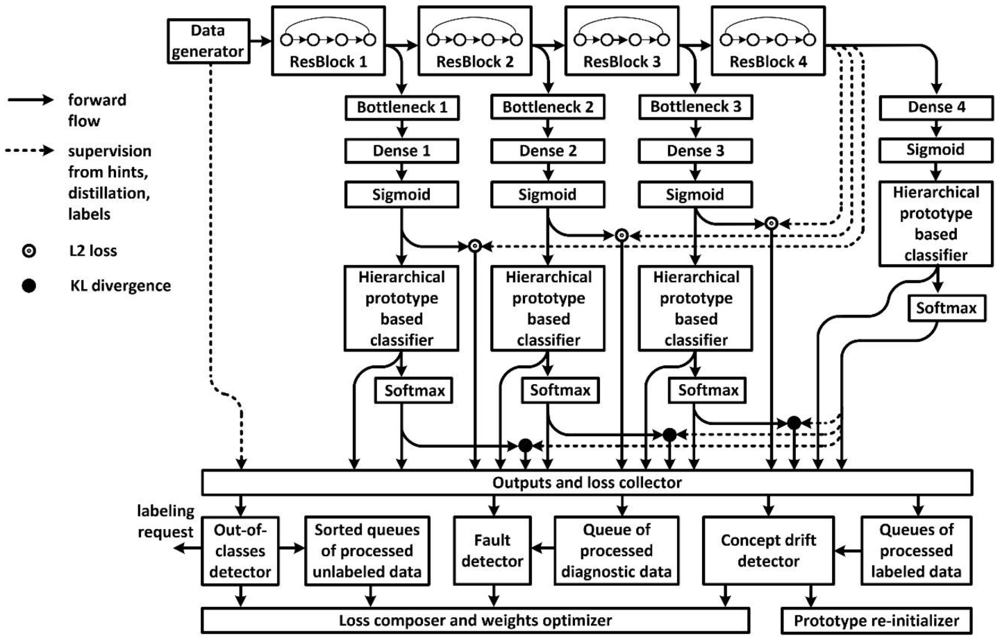
3. Classification Model Design

3.1. Principles

When building the model, we aim to implement the main characteristics of resilience: robustness, graceful degradation, recovery, and improvement. The model is based on the following principles:

-

hierarchical labeling and hierarchical classification to implement the principle of graceful degradation by coarsening the prediction with a more abstract class and with reasonable confidence when classes at the bottom of the hierarchy are recognized with a low confidence level;

-

combining the mechanisms of self-knowledge distillation and nested learning to increase the robustness of the model by increasing the informativeness of the feedback for the lower layers at the training stage and accelerate inference by skipping high-level layers for simple samples at the inference stage;

-

prototype and compact spherical container formation for each class to simplify the detection of out-of-distribution samples and concept drifts;

-

using memory FIFO queues with a limited size to store labeled and unlabeled data with corresponding values of loss function obtained by inference for implementation diagnostic and recovery mechanism.

These principles should ensure resource efficiency because the model will have small branches for intermediate decisions which introduces minimal redundancy, since the main part of the feature extractor body is shared between intermediate classifiers. In addition, the size of data queues for diagnostic samples with corresponding loss, or labeled and unlabeled samples with the result of their recognition, can be set to an acceptable capacity from the point of view of resource constraints.

3.2. Architecture

Figure 1 depicts the architecture of the resilient classifier.

It illustrates the sectional design of the deep neural classifier. Sections consist of ResBlocks of the well-known ResNet50 architecture. The ResNet50 architecture also provided the inspiration for the Bottleneck module, serving to mitigate the impacts between each classifier of the lower sections, and to add distillation knowledge from the high-level feature map to the lower-level feature maps. The output of each section is used to construct a separate classifier. Each classifier receives feedback from the data labels and the last layer. Feedback from the last layer, denoted by a dotted line, ensures the implementation of the principle of self-knowledge distillation.

A set of prototype vectors is constructed for the classification analysis of the feature representation of each section output. Prototype vectors are not fixed; they are tuned in the training process together with weights of the feature extractor. To implement the graceful degradation principle, prototypes can belong to different levels in the hierarchy, according to the hierarchy of labeling. In the example provided, a two-level hierarchy is used. To increase immunity to noise and implement the information bottleneck, we approximate the feature representation to a discrete form, which is why the output of the feature extractor of each section uses the sigmoid layer and the corresponding regularization in the training algorithm.

The radius of hyperspherical containers of classes is optimized for each prototypical classifier. Container radii are stored in memory to detect high levels of uncertainty when making decisions. Test samples outside the class containers become candidates for semi-supervised tuning and for manual labeling (active learning) to be performed at a later stage. Controlling for the samples outside the class container can also be used for real concept drift and out-of-distribution detection.

After updating the weights and parameters of the model, the diagnostic dataset and the corresponding value of the loss function must be stored (or updated) in memory. After that, a subset of diagnostic data should be passed along for inference purposes, together with the test samples in each batch. This will allow a comparison of the past and present values of the loss function to detect errors or injection faults in the memory of the neural network weights. Where the difference between past and present values of the loss function exceeds a certain threshold $\mathsf{\alpha }=0.01$, a neural network fine-tuning algorithm utilizing the diagnostic data needs to be initiated to bring this difference under a threshold $\mathsf{\beta }=0.001$.

The multi-section structure of the model with intermediate classifiers allows adaptive calculations to be implemented and the recognition of simple images to be accelerated. At the same time, as the model is continually trained, it becomes faster due to increased prediction confidence of the lower section classifiers. This, in turn, will allow the rest of the high-level sections of the model to be skipped. The following rules for classification analysis in the adaptive calculations framework are proposed:

-

neural network calculations are performed sequentially, section by section;

-

high-level sections can be skipped if the maximal value of the membership function in the output of the current section, with regards to a particular class of the lower hierarchical level, exceeds the confidence threshold $\mathrm{T}$;

-

if the maximal value of the membership function of any of the hierarchical levels of the classifier at the output of the current section has not increased compared to the previous section, the subsequent calculations can be omitted;

-

where any of the conditions of omission of the subsequent sections are fulfilled or the classifier in question is the last classifier in the model and the maximal value of the membership function of the lower hierarchical level does not exceed the confidence threshold, a higher level in the hierarchy is checked;

-

where a class with a sufficient confidence level has not been identified, a decision is refused, a request for a manual labeling is generated, and the corresponding sample is designated as suitable for semi-supervised tuning.

The hierarchical prototype-based classifier module consists of class prototypes, hyperspherical container parameters, and parameter regularization intended to compress (discretize) feature representation and prototypes. In this case, the confidence in the forecast of the $\mathrm{i}$-th sample belonging to the $\mathrm{k}$-th class, is determined by the following membership function [28,29,52]

$${\mathsf{\mu }}_{\mathrm{k}}\left({\mathrm{z}}_{\mathrm{i}}\right)=1-\frac{\mathrm{dist}\left({\mathrm{z}}_{\mathrm{i}},{ \overline{\mathrm{z}}}_{\mathrm{k}}\right)}{\mathrm{N}·{\mathrm{r}}_{\mathrm{k}}},$$

(1)

where ${\mathrm{z}}_{\mathrm{i}}$ is a binarized feature representation of $\mathrm{i}$-th example at the feature extractor output;

${ \overline{\mathrm{z}}}_{\mathrm{k}}$ is a trainable $\mathrm{k}$-th class prototype;

$\mathrm{N}$ is a dimension of input feature vector ${\mathrm{z}}_{\mathrm{i}}$;

${\mathrm{r}}_{\mathrm{k}}$ is a trainable scale factor for the radius of hyperspherical decision boundary (container) of the $\mathrm{k}$-th class, ${\mathrm{r}}_{\mathrm{k}}\in \left(0;1\right)$;

$\mathrm{dist}\left(·\right)$ is a Euclidean squared distance.

If the maximum value of Function (1) for an input unlabeled sample ${\mathrm{z}}_{\mathrm{i}}$ is less than zero, such a forecast should not be trusted and such a sample should be added to the queue of unlabeled data outside the training distribution. Where the input unlabeled sample falls into one of the containers of the recognition classes (at any of the levels), it should be added to the in-class unlabeled data buffer within the training distribution. Unlabeled sample buffers can be used for training with pseudo-labeling and soft-labeling, or for consistency regularization.

Where the model is trained, but an occurrence of $\mathrm{n}$ samples of the $\mathrm{c}$-th class misallocated during forward propagation to $\mathrm{k}$-th class container is detected in the queue of the new labeled data, the real concept drift is recognized.

To avoid catastrophic forgetting in the context of concept drifts or the emergence of a new recognition class, a reminder function is implicitly implemented. Such a function is based on unlabeled data queues and prototypical vectors in feature space, which are changing slowly. Upper-layer knowledge distillation mechanism also serves the same purpose.

Data from the unlabeled data queue can be moved to the labeled data queue after the feedback on their actual affiliation with the classes is received. The priority of specific samples being recommended for manual labeling depends on the value of the membership Function (1).

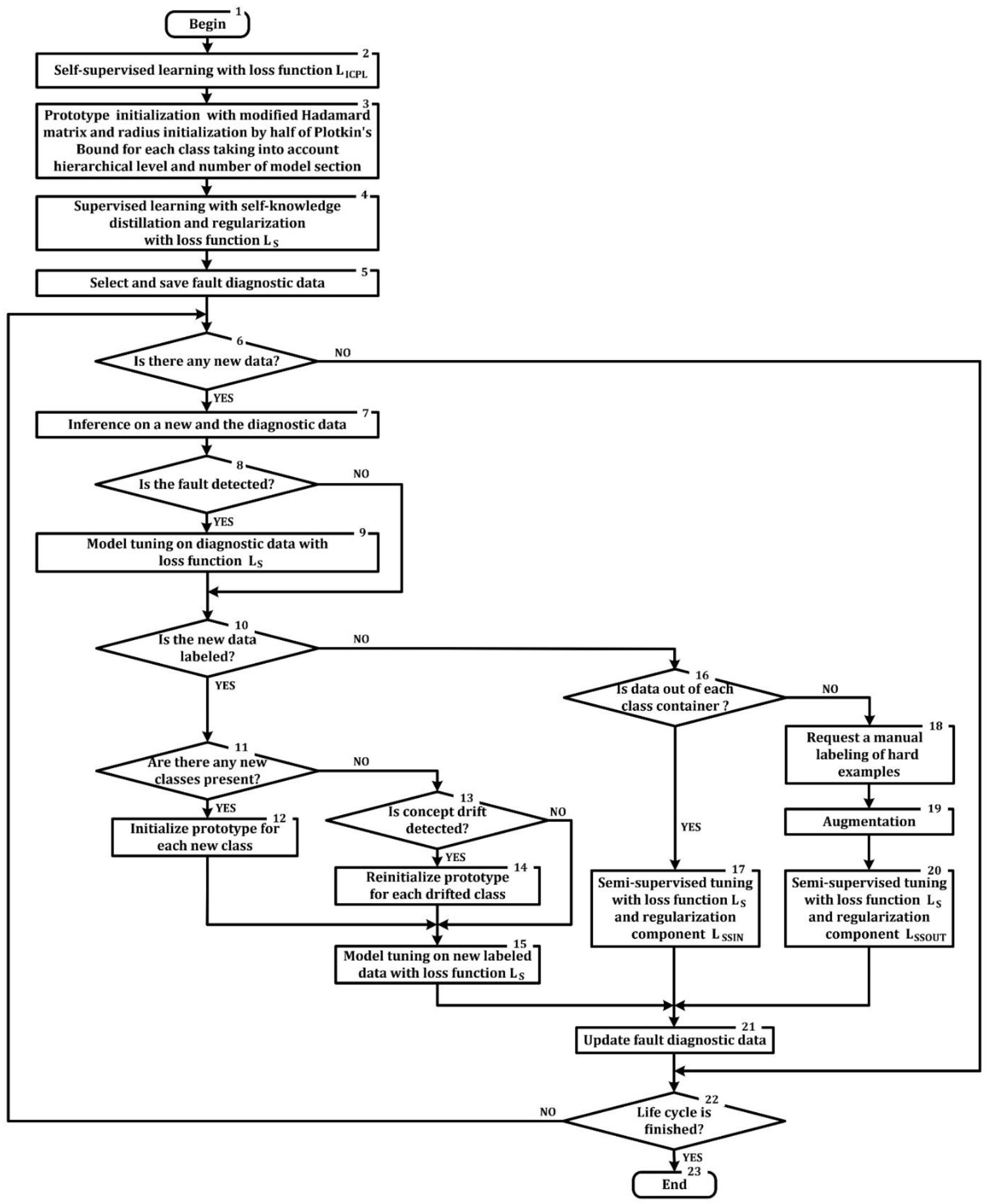
4. Training Method Design

4.1. Principles

During the development of the training method, we aim to ensure robustness, graceful degradation, recovery, and improvement. To this end, the training algorithm will be based on the following principles:

-

accounting for the hierarchy of data labeling and hierarchy class prototypes by calculating the loss function separately for each level of the hierarchy to provide graceful degradation at the inference;

-

the implementation of self-knowledge distillation, i.e., distillation of knowledge from the high-level layer (section) of the model down to lower layers (sections) as additional regularization components to increase robustness and provide adaptive calculations in inference mode;

-

increasing the compactness of the distribution of classes and the buffer zone between classes to increase resistance to noise, outliers, and adversarial attacks in turn as an additional distance-based regularization component;

-

the discretization of feature representation in order to implement the information bottleneck and increase the robustness of the feature representation as an additional regularization component;

-

the ability to effectively use both labeled and unlabeled data samples to speed up adaptation with a limited quantity of labeled data, which usually comes with a time lag;

-

the avoidance of catastrophic forgetting when adapting to change and adversarial attacks without full retraining by implementing a reminding mechanism which utilizes the data buffers and distillation feedback of the upper layers.

4.2. Stages

The proposed training method consists of the following stages:

-

self-supervision pre-training of the model with instance-prototype contrastive loss ${\mathrm{L}}_{\mathrm{ICPL}}$;

-

prototype and radius initialization for each class;

-

supervised learning with loss function ${\mathrm{L}}_{\mathrm{S}}$, which includes conventional cross-entropy and additional components for self-knowledge distillation and regularization;

-

selecting fault diagnostic data (selected randomly or with respect to the value of the loss function);

-

inference on a new and diagnostic data;

-

requesting manual labeling of hard examples;

-

supervised learning with loss function ${\mathrm{L}}_{\mathrm{S}}$, taking into account manual labeling responses or semi-supervised fine-tuning (adaptation) with additional component ${\mathrm{L}}_{\mathrm{SSIN}}$ or ${\mathrm{L}}_{\mathrm{SSOUT}}$ depends on the result of inference;

-

updating diagnostic data.

Where a large amount of unlabeled data is available, the model preparation should start with self-supervised learning of feature extractor. For this purpose, it is proposed to use instance-prototype contrastive loss, characterized by computational efficiency and generalizing ability close to the biological prototype [53]. Instance-prototype contrastive loss is calculated by the formula

$${\mathrm{L}}_{\mathrm{ICPL}}=-\log \frac{\exp \left(-\mathrm{dist}\left({\mathrm{z}}_{\mathrm{i}},{ \overline{\mathrm{z}}}_{\mathrm{i}}\right)/\mathsf{\tau }\right)}{\exp \left(-\mathrm{dist}\left({\mathrm{z}}_{\mathrm{i}},{ \overline{\mathrm{z}}}_{\mathrm{i}}\right)/\mathsf{\tau }\right)+{{\displaystyle \sum }}_{\mathrm{b}=1}^{\mathrm{B}}\exp \left(-\mathrm{dist}\left({\mathrm{z}}_{\mathrm{i}},{ \mathrm{z}}_{\mathrm{b}}\right)/\mathsf{\tau }\right)},$$

(2)

where ${\mathrm{z}}_{\mathrm{i}}$ is a feature representation at the output of the feature extractor ${\mathrm{z}}_{\mathrm{i}}=\mathrm{f}\left({\mathrm{x}}_{\mathrm{i}}\right)$ for input example ${\mathrm{x}}_{\mathrm{i}}$ from a mini-batch;

${ \overline{\mathrm{z}}}_{\mathrm{i}}$ represents an averaged feature representation for the augmented version of input example and considered as a positive pair for the input example ${\mathrm{x}}_{\mathrm{i}}$,

$${ \overline{\mathrm{z}}}_{\mathrm{i}}=\frac{1}{{\mathrm{n}}_{\mathrm{a}}}{\displaystyle \sum }_{\mathrm{j}=1}^{{\mathrm{n}}_{\mathrm{a}}}\mathrm{f}\left({\mathrm{a}}_{\mathrm{j}}\left({\mathrm{x}}_{\mathrm{i}}\right)\right),$$

(3)

where ${\mathrm{a}}_{\mathrm{j}}$ is an augmentation operator, such as random cropping, rescaling, random horizontal/vertical flip, random adjustment to hue, saturation, contrast and brightness, and random grayscale conversion;

$\mathrm{B}$ is the number of pre-processed examples considered as negative pairs, the feature representations of which are stored in the non-indexed FIFO queue (with queue length $\mathrm{B}=1024$) and updated after the processing of each mini-batch;

$\mathsf{\tau }$ is a temperature parameter that controls the dynamic range of the similarity function.

The loss function ${\mathrm{L}}_{\mathrm{S}}$ used in supervised learning includes, in addition to the conventional cross-entropy ${\mathrm{L}}_{\mathrm{SCE}}$ computed with labels and predictions, a class-level component ${\mathrm{L}}_{\mathrm{CSD}}$ and a feature-level component ${\mathrm{L}}_{\mathrm{FSD}}$ of self-knowledge distillation. A regularization component ${\mathrm{L}}_{\mathrm{D}}$ can also be added to the loss function in order to achieve compression of feature representation, implementing an information bottleneck principle. The contrastive-center loss ${\mathrm{L}}_{\mathrm{CCL}}$ can be used as a regularization component to enhance robustness optimization by increasing intra-class compactness and inter-class separability. Thus, the following combined loss function is suggested for supervised learning

$${\mathrm{L}}_{\mathrm{S}}={\mathsf{\lambda }}_{\mathrm{SCE}}{ \overline{\mathrm{L}}}_{\mathrm{SCE}}+{\mathsf{\lambda }}_{\mathrm{CCL}}{ \overline{\mathrm{L}}}_{\mathrm{CCL}}+{\mathsf{\lambda }}_{\mathrm{CSD}}{ \overline{\mathrm{L}}}_{\mathrm{CSD}}+{\mathsf{\lambda }}_{\mathrm{FSD}}{ \overline{\mathrm{L}}}_{\mathrm{FSD}}+{\mathsf{\lambda }}_{\mathrm{D}}{ \overline{\mathrm{L}}}_{\mathrm{D}},$$

(4)

where ${ \overline{\mathrm{L}}}_{\mathrm{SCE}}$ and ${ \overline{\mathrm{L}}}_{\mathrm{CCL}}$ represent the values of the respective loss functions ${\mathrm{L}}_{\mathrm{SCE}}$ and ${\mathrm{L}}_{\mathrm{CCL}}$ averaged over $\mathrm{S}$-sections and $\mathrm{H}$-levels of the hierarchy of classes of the classification model;

${ \overline{\mathrm{L}}}_{\mathrm{FSD}}$ and ${ \overline{\mathrm{L}}}_{\mathrm{CSD}}$ represent the values of the respective loss functions ${\mathrm{L}}_{\mathrm{FSD}}$ and ${\mathrm{L}}_{\mathrm{CSD}}$ averaged over $\left(\mathrm{S}-1\right)$-sections and $\mathrm{H}$-levels of the hierarchy of classes of the classification model;

${ \overline{\mathrm{L}}}_{\mathrm{D}}$ is averaged by $\mathrm{S}$-outputs (sections) of the classification model, including the output of the last layer and the value of the loss function ${\mathrm{L}}_{\mathrm{D}}$;

${\mathsf{\lambda }}_{\mathrm{SCE}}$, ${\mathsf{\lambda }}_{\mathrm{CCL}}$, ${ \mathsf{\lambda }}_{\mathrm{FSD}}$, ${ \mathsf{\lambda }}_{\mathrm{CSD}}$, and ${ \mathsf{\lambda }}_{\mathrm{D}}$ are the coefficients for regulating the influence of the components of the resulting loss function.

The classifier module is proposed to be built on the basis of class prototypes, which are the centers of hyperspherical containers. In this case, the cross-entropy loss ${\mathrm{L}}_{\mathrm{SCE}}$ is calculated at the output of the classifier by the formula

$${\mathrm{L}}_{\mathrm{SCE}}=\mathrm{CE}\left(\mathrm{q}\left({\mathrm{z}}_{\mathrm{i}}, \mathsf{\tau }=1\right),{ \mathrm{y}}_{\mathrm{i}}\right),$$

(5)

where $\mathrm{CE}\left(·\right)$ is the cross-entropy loss function;

${\mathrm{y}}_{\mathrm{i}}$ is a one-hot encoded vector of the target variable for the $\mathrm{i}$-th input sample;

$\mathrm{q}\left(·\right)$ is an assessment of the probability of belonging to the feature representation of the $\mathrm{i}$-th sample to a particular class container, which for the $\mathrm{k}$-th class is calculated by the formula

$${\mathrm{q}}_{\mathrm{k}}\left({\mathrm{z}}_{\mathrm{i}}, \mathsf{\tau }\right)=\mathrm{softmax}{\left(\mathrm{leaky}\_\mathrm{relu}\left(\mathsf{\mu }\left({\mathrm{z}}_{\mathrm{i}}\right)/\mathsf{\tau }\right)\right)}_{\mathrm{k}}=\frac{\exp \left(\mathrm{leaky}\_\mathrm{relu}\left({\mathsf{\mu }}_{\mathrm{k}}\left({\mathrm{z}}_{\mathrm{i}}\right)/\mathsf{\tau }\right)\right)}{{{\displaystyle \sum }}_{\mathrm{c}=1}^{\mathrm{K}}\exp \left(\mathrm{leaky}\_\mathrm{relu}\left({\mathsf{\mu }}_{\mathrm{c}}\left({\mathrm{z}}_{\mathrm{i}}\right)/\mathsf{\tau }\right)\right)},$$

(6)

where $\mathrm{K}$ is a size of the class set;

$\mathrm{leaky}\_\mathrm{relu}$ is an improved version of the ReLU function with a small slope (alpha = 0.02) for negative values.

Contrastive-center loss function ${\mathrm{L}}_{\mathrm{CCL}}$, which impacts the optimization efficiency of each class prototype, is calculated on a labeled training set by the formula [10]

$${\mathrm{L}}_{\mathrm{CCL}}=\frac{\mathrm{dist}\left({\mathrm{z}}_{\mathrm{i}},{ \overline{\mathrm{z}}}_{{\mathrm{y}}_{\mathrm{i}}}\right)}{{{\displaystyle \sum }}_{\mathrm{k}=1, \mathrm{k}\ne {\mathrm{y}}_{\mathrm{i}}}^{\mathrm{K}}\mathrm{dist}\left({\mathrm{z}}_{\mathrm{i}},{ \overline{\mathrm{z}}}_{\mathrm{k}}\right)+1}.$$

(7)

Self-knowledge distillation components, such as ${\mathrm{L}}_{\mathrm{FSD}}$ in the form of ${\mathrm{L}}_2$ loss from hints and ${\mathrm{L}}_{\mathrm{CSD}}$ in the form of Kullback–Leibler divergence loss, are calculated based on the $\mathrm{S}$-th (last) output of the model and the $\mathrm{s}$-th output (intermediate) of the model

$${\mathrm{L}}_{\mathrm{FSD}}=\mathrm{dist}\left({\mathrm{z}}_{\mathrm{i}}^{\mathrm{s}},{ \mathrm{z}}_{\mathrm{i}}^{\mathrm{S}}\right),$$

(8)

$${\mathrm{L}}_{\mathrm{CSD}}=\mathrm{KL}\left(\mathrm{q}({\mathrm{z}}_{\mathrm{i}}^{\mathrm{s}},\mathsf{\tau }\right), \mathrm{q}({\mathrm{z}}_{\mathrm{i}}^{\mathrm{S}},\mathsf{\tau })),$$

(9)

where ${\mathrm{z}}_{\mathrm{i}}^{\mathrm{s}}$, ${\mathrm{z}}_{\mathrm{i}}^{\mathrm{S}}$ is the feature representation at the output of the $\mathrm{s}$-th section (intermediate output) of the model and at the $\mathrm{S}$ output (last output) model.

A regularization component ${\mathrm{L}}_{\mathrm{D}}$ implements the information bottleneck by penalizing the discretization error of feature representation

$${\mathrm{L}}_{\mathrm{D}}={\mathrm{z}}_{\mathrm{i}}{}^{\mathrm{T}}\left(\mathrm{e}-{\mathrm{z}}_{\mathrm{i}}\right),$$

(10)

where $\mathrm{e}$ is a unit vector.

To speed up adaptation to changes, unlabeled data examples can be used in consistency regularization [50]. In this case, unlabeled data are divided into two groups: unlabeled examples, which fall into the class containers, and unlabeled examples, which are outside all class containers.

Unlabeled examples which fall into class containers, are used to calculate regularization component ${\mathrm{L}}_{\mathrm{SSIN}}$ by the following formula

$${\mathrm{L}}_{\mathrm{SSIN}}=\mathrm{CE}\left(\mathrm{q}({\mathrm{z}}_{\mathrm{i}}^{\prime },\mathsf{\tau }=1), \mathrm{q}({\mathrm{z}}_{\mathrm{i}}^{″},\mathsf{\tau }=1)\right),$$

(11)

where ${\mathrm{z}}_{\mathrm{i}}^{\prime }$, ${\mathrm{z}}_{\mathrm{i}}^{″}$ are feature presentations of two augmented versions of the input sample ${\mathrm{x}}_{\mathrm{i}}$.

Certain portions γ (≤10%) of unlabeled data, which fall into class containers and have maximum values of $\mathrm{q}\left({\mathrm{z}}_{\mathrm{i}}\right)$, can be pseudo-labeled with the corresponding classes. Such pseudo-labeled data can be included in every mini-batch during training.

Unlabeled examples which fall outside of all class containers, may be examples of unknown classes or concept drift results. In this case, soft-labeling ${\mathrm{q}}_{\mathrm{k}}^{\mathrm{dist}}\left({\mathrm{z}}_{\mathrm{i}}\right)$ based on distances to prototype of known classes should be used in the consistency regularization component ${\mathrm{L}}_{\mathrm{SSOUT}}$:

$${\mathrm{L}}_{\mathrm{SSOUT}}=\mathrm{CE}\left(\mathrm{q}\left({\mathrm{z}}_{\mathrm{i}},\mathsf{\tau }=1\right),{ \mathrm{q}}^{\mathrm{dist}}\left({\mathrm{z}}_{\mathrm{i}}\right)\right)$$

(12)

$${\mathrm{q}}_{\mathrm{k}}\left({\mathrm{z}}_{\mathrm{i}}\right)=\mathrm{softmax}{\left(-\mathrm{dist} \left({\mathrm{z}}_{\mathrm{i}}, \overline{\mathrm{z}}\right)\right)}_{\mathrm{k}}=\frac{\exp \left(-\mathrm{dist}\left({\mathrm{z}}_{\mathrm{i}},{ \overline{\mathrm{z}}}_{\mathrm{k}}\right)\right)}{{{\displaystyle \sum }}_{\mathrm{c}=1}^{\mathrm{K}}\exp \left(-\mathrm{dist}\left({\mathrm{z}}_{\mathrm{i}},{\overline{ \mathrm{z}}}_{\mathrm{c}}\right)\right)}.$$

(13)

Figure 2 shows a block diagram of the proposed algorithm for training image classifier with resilience to adversarial attacks, fault injection, and concept drifts.

Algorithm execution steps 2 to 5 are responsible for the preparation phase of the resilient image classifier. Algorithm execution steps 6 to 20 are related to the collection of new data and adaptation to perturbations. The adaptation process is continuous until the end of the classifier life cycle.

Step 3, step 13, and step 15 of the algorithm (Figure 2) are quite important, since the efficiency of the classifier depends on their implementation. These steps aim to initialize or re-initialize the prototype and container radius for each class. The initial values of the parameters of the lower-level class prototypes are initialized on the basis of the Hadamard matrix [22] using the principle of label smoothing. For this, first, the dimensionality of the Hadamard matrix is determined ${\mathrm{N}}_{\mathrm{Hadamard}}=2^{\mathrm{ceil}\left({\log }_2\left(\mathrm{N}\right)\right)}$, where $\mathrm{ceil}()$ is the function rounding a number to a larger integer value. All values less than 0 are replaced by 0, i.e., $\mathrm{Z}=\max \left(0, \mathrm{Hadamard}\left({\mathrm{N}}_{\mathrm{Hadamard}}\right)\right)$ subsequently.

As the next step, to facilitate the process of adapting the class prototype to the data structure, the proposed approach uses label smoothing. This is performed according to the formula $\mathrm{Z}\prime =\mathrm{Z}·0.7+0.15$; as a result, the 1′ s will turn into 0.87, and the 0′ s into 0.15. K of the first vectors truncated by N first features, i.e., $\overline{\mathrm{z}}=\mathrm{Z}\prime \left[1:\mathrm{K}, 1:\mathrm{N}\right]$, are then selected from the resulting matrix. The trainable scale factor ${\mathrm{r}}_{\mathrm{k}}$ for the radius of the hyperspherical decision boundary (container) of the $\mathrm{k}$-th class is initialized with a value of half of the Plotkin bounds, divided by the dimensionality of the feature space [29,54].

$${\mathrm{r}}_{\mathrm{k}}\leftarrow \left(\frac{1}{2}\frac{\mathrm{N}}{2}\frac{\mathrm{K}}{\mathrm{K}-1}\right)\frac{1}{\mathrm{N}}=\frac{\mathrm{K}}{4\left(\mathrm{K}-1\right)}.$$

(14)

The appearance of a sample with a label indicating a new ($\mathrm{K}+1)$-th lower-level class necessitates the formation of a new prototype for the class ${\mathrm{Z}}_{\mathrm{K}+1}$ with the corresponding initial values of the radius scale factor ${\mathrm{r}}_{\mathrm{K}+1}$. This is achieved by selecting the nearest vector from the remaining unused rows of a modified Hadamard matrix $\mathrm{Z}\prime$, where the proximity is determined on the basis of Euclidean squared distance. The initial value of the radius scale factor for the new class is also determined by Formula (14), but taking into account the new number of classes.

Each coordinate of the prototype of the upper hierarchical level is initialized by copying the corresponding coordinate of one of the prototypes of the lower level, selected at random. The initial class radius of the upper hierarchical level is determined by Formula (14), taking into account the number of classes at this level.

When a real concept drift is recognized, prototypes of drifting classes are populated with random numbers from the range between 0 and 1.

Diagnostic datasets are formed by sampling labeled examples which fall into their class containers according to inference results. This is represented by step 5 and step 21 of the algorithm depicted on Figure 2. The value of loss Function (4), calculated for the diagnostic data, is stored in the memory for comparison purposes. When a mismatch is detected between the current value and the previously calculated value of the loss function, fine-tuning takes place. Fine-tuning is stopped if the difference is reduced by more than 10 times.

5. Experiments

The CIFAR-10 and CIFAR-100 datasets are chosen for experimentation because the datasets are publicly available and their images are small in size, which speeds up experimental research [55,56]. Classes of the CIFAR-10 dataset can be arranged in a hierarchical structure. For example, the first superclass (upper level class) will be the animal class, which includes the bird, cat, deer, dog, frog, and horse subclasses. The second superclass will be the vehicle class, which includes the airplane, automobile, ship, and truck subclasses. The CIFAR-10 dataset consists of 50,000 training images and 10,000 test 32 × 32 color images distributed evenly between 10 classes. The 100 classes in the CIFAR-100 are grouped into 20 superclasses at the first upper level [55]. The CIFAR-100 consists of the same number of images as the CIFAR-10, but has 500 training images per class and 100 test images per class. For convenience of the analysis, for training of the base model, we will use 70% of training data to form a dataset base, and use the remaining 30% for the additional training dataset.

In the case of the CIFAR-10 dataset, 12 prototype vectors will be used at the output of the classifier of each section, of which 2 are used for superclass prototypes and 10 are used for lower-level prototypes. In the case of the CIFAR-100 dataset, 120 prototype vectors will be used at the output of the classifier of each section, respectively.

For all experiments, the chosen confidence threshold, considered sufficient to make a decision, is $\mathrm{T}=0.8$. The training is carried out on the basis of the Adam optimizer with a learning rate equal to 0.0003. The dimension of feature representation is set to 64 ($\mathrm{N}=64$). Default values of coefficients used in loss Function (4) are proposed as follows: ${\mathsf{\lambda }}_{\mathrm{SCE}}=1.0$, ${\mathsf{\lambda }}_{\mathrm{CCL}}=1.0$, ${\mathsf{\lambda }}_{\mathrm{CSD}}=0.1$, ${ \mathsf{\lambda }}_{\mathrm{FSD}}=0.01$, ${ \mathsf{\lambda }}_{\mathrm{D}}=0.0001$. Besides that, semi-supervision components ${\mathrm{L}}_{\mathrm{SSIN}}$ and ${\mathrm{L}}_{\mathrm{SSOUT}}$ are used with coefficients ${\mathsf{\lambda }}_{\mathrm{SSIN}}=0.1$ and ${\mathsf{\lambda }}_{\mathrm{SSOUT}}=0.1$, respectively. Preliminary training with the loss Function (2) is proposed to be carried out on all the training data, disregarding the labels. The size of the proposed mini-batch is 128 images.

Different model weights have different importance and varying levels of impact on model performance. In addition, a fault in the higher bits of tensor value leads to a greater distortion of the results than a fault in the lower bits. Similarly, the effectiveness of adversarial attacks with the same amplitude constraint can be very different depending on the spatial distribution of the perturbed pixels. Therefore, statistical characteristics should be used to evaluate and compare the model’s resilience to damaged tensors or perturbed images. The statistical characteristics are derived from a large number of experiments, where bits and tensors for inversion are chosen randomly from a uniform distribution or adversarial images generated by black-box optimizer with randomized evolution strategy. For simplicity, we can consider the median (MED) value and the interquartile (IRQ) value of the classifier’s accuracy (Acc) or precision (Prec) under perturbation and the required number of performance recovery steps (Rec_steps), calculated after 1000 experiments.

To test the model for fault tolerance and resiliency, the TensorFI2 library is recommended, which is able to emulate software and hardware failures [57]. The experiment proposes to consider the effect of the most difficult-to-absorb type of failure—a bit-flip injection in each layer of the model layer, with randomly selected fixed tensor fraction (fault rate) and one randomly selected bit for inversion. Diagnostic data are added to each model for diagnostics and recovery, together with test data at the model input.

For the ease of simulation, it is assumed that fault injection is generated anew before feeding each training mini-batch. Diagnostic data are selected from the dataset additional set and the data quantity is equal to the size of 128 images. The recovery process stops when the loss function on the diagnostic data does not decrease for five consecutive iterations, or when difference between past and present values of the loss function is less than $\mathsf{\beta }=0.001$.

Table 2. A comparison of the accuracy under fault injection and required number of performance recovery steps.

Dataset	Fault Rate	MED (Acc) Under Fault Injection	MED (Acc) After Recovery	MED (Acc) for Superclass Level Under Fault Injection	MED (Acc) for Superclass Level After Recovery	MED (Rec_Steps)	MED (Rec_Steps) for Superclass Level
CIFAR-10	0.0	0.993	-	0.980	-	-	-
CIFAR-10	0.1	0.985	0.991	0.975	0.979	12	12
CIFAR-10	0.2	0.932	0.976	0.930	0.961	29	21
CIFAR-10	0.3	0.852	0.971	0.870	0.932	32	32
CIFAR-10	0.4	0.801	0.921	0.790	0.914	49	54
CIFAR-10	0.5	0.713	0.882	0.730	0.893	63	71
CIFAR-10	0.6	0.532	0.851	0.721	0.881	81	80
CIFAR-100	0.0	0.890	-	0.970	-	-	-
CIFAR-100	0.1	0.879	0.889	0.962	0.970	35	25
CIFAR-100	0.2	0.871	0.881	0.961	0.970	55	51
CIFAR-100	0.3	0.790	0.880	0.926	0.961	59	50
CIFAR-100	0.4	0.600	0.870	0.910	0.958	62	64
CIFAR-100	0.5	0.551	0.851	0.890	0.929	70	71
CIFAR-100	0.6	0.357	0.758	0.665	0.910	80	77

shows the dependency of models’ accuracy before and after recovery on fault rate for the class and superclass hierarchical levels, regardless of which the model section’s output is chosen as final. The table also contains the number of steps performed to recover in each case. In all experiments, the presence of faults is detected with 100% accuracy.

Table 2 shows that a higher hierarchical classifier absorbs faults better and recovers better on diagnostic data, although a higher hierarchical-level classifier carries less information. This is an useful property for the mechanism of graceful degradation. At the same time, in the presence of a single random bit-flip in 10% of the randomly selected tensors of the deep model, the accuracy of the classifier of the lower and upper hierarchical level did not change noticeably, which is a manifestation of the robustness property. A further increase in the fault rate leads to a noticeable decrease in accuracy, but recovery mechanism recovers more than half of the accuracy drop.

It is also noticed that as the fault rate increases, the number of recovery iterations increases. The IRQ of the calculated accuracy values does not exceed 0.05, and the IRQ of the recovery step number does not exceed 9. At the same time, the difference in the number of classes in the CIFAR-10 and CIFAR-100 datasets did not have a significant impact on the behavior of the classifier.

To test the model for resilience to noise and adversarial attacks, it is suggested not to rely on the specific features of the model architecture and learning algorithm, such as gradients. Testing instead would be based on black-box attacks. In this case, we will consider two types of attacks that give the most divergent results—one/few pixels for “strong” attacks and all pixels for “slight” attacks. The formation of both attacks will be implemented on the basis of the covariance matrix adaptation evolution strategy (CMA-ES) search algorithm [58]. For the first type of attacks, the constraint on the perturbation amplitude ($\mathrm{th}$) is set by the ${\mathrm{L}}_0$-norm and for the second by the ${\mathrm{L}}_{\infty }$-norm.

Table 3. A comparison of the accuracy under adversarial perturbations.

Dataset	Threshold for Perturbation Level	MED (Acc) on Perturbed Test Data		MED (Acc) for Superclass Level on Perturbed Test Data		MED (Prec) on Perturbed Test Data		MED (Prec) for Superclass Level on Perturbed Test Data
		${\mathbf{L}}_0$- Attack	${\mathbf{L}}_{\mathit{\infty }}$- Attack	${\mathbf{L}}_0$- Attack	Linf- Attack	${\mathbf{L}}_0$- Attack	Linf- Attack	${\mathbf{L}}_0$- Attack	Linf- Attack
CIFAR-10	0	0.981	0.981	0.995	0.995	0.981	0.981	0.995	0.995
CIFAR-10	1	0.975	0.967	0.980	0.970	0.979	0.978	0.991	0.991
CIFAR-10	2	0.941	0.853	0.965	0.881	0.978	0.977	0.991	0.990
CIFAR-10	3	0.851	0.762	0.880	0.811	0.977	0.975	0.989	0.984
CIFAR-10	4	0.831	0.744	0.875	0.771	0.977	0.974	0.985	0.980
CIFAR-10	5	0.801	0.711	0.871	0.741	0.963	0.955	0.985	0.979
CIFAR-10	6	0.781	0.680	0.841	0.711	0.950	0.949	0.973	0.970
CIFAR-100	0	0.890	0.890	0.970	0.970	0.930	0.930	0.980	0.980
CIFAR-100	1	0.885	0.883	0.970	0.967	0.930	0.926	0.978	0.971
CIFAR-100	2	0.881	0.880	0.942	0.941	0.910	0.910	0.972	0.968
CIFAR-100	3	0.833	0.829	0.910	0.900	0.905	0.900	0.970	0.941
CIFAR-100	4	0.741	0.745	0.902	0.871	0.898	0.889	0.960	0.941
CIFAR-100	5	0.692	0.701	0.820	0.812	0.891	0.884	0.920	0.905
CIFAR-100	6	0.642	0.603	0.780	0.750	0.890	0.883	0.820	0.831

shows the dependence of the model accuracy and precision on the perturbed test data with different maximum perturbation amplitudes ($\mathrm{th}$), according to the ${\mathrm{L}}_0$ and ${\mathrm{L}}_{\infty }$ norms for the upper and lower hierarchical levels, respectively.

Table 3 shows that the upper hierarchical level absorbs perturbations from adversarial attacks better, while the accuracy decreases more under the influence of ${\mathrm{L}}_{\infty }$ attacks. Analysis of the accuracy values shows that the trained classifier is quite robust to the attacks with a maximum amplitude of $\mathrm{th}=1$. The sharpest decline in accuracy occurs for $\mathrm{th}>3$. Analysis of the precision values shows that an increase in the level of perturbation mainly leads to an increase in the number of reject decisions, rather than false positives. The high precision can be regarded as one of the forms of graceful degradation.

The recovery of performance under adversarial perturbations takes place continuously through semi-supervised learning. The queue of the last labeled data can be updated by active learning mechanisms. The perturbed dataset, with 10% labeled and 90% unlabeled examples, is used to simulate active learning mechanism.

Table 4. A comparison of the required number of performance recovery steps.

Dataset	Threshold for Perturbation Level	MED (Rec_Steps)		MED (Rec_Steps) for Superclass Level		IRQ (Rec_Steps)		IRQ (Rec_Steps) for Superclass Level
		${\mathbf{L}}_0$- Attack	${\mathbf{L}}_{\mathit{\infty }}$- Attack	${\mathbf{L}}_0$- Attack	${\mathbf{L}}_{\mathit{\infty }}$- Attack	${\mathbf{L}}_0$- Attack	${\mathbf{L}}_{\mathit{\infty }}$- Attack	${\mathbf{L}}_0$- Attack	${\mathbf{L}}_{\mathit{\infty }}$- Attack
CIFAR-10	1	12	18	10	13	1	2	2	2
CIFAR-10	2	21	29	20	21	1	1	3	3
CIFAR-10	3	32	45	31	35	2	3	2	5
CIFAR-10	4	39	50	39	42	3	3	4	4
CIFAR-10	5	50	68	41	44	2	6	3	7
CIFAR-10	6	91	111	59	52	4	5	5	6
CIFAR-100	1	34	37	20	22	3	3	4	4
CIFAR-100	2	39	41	42	42	5	3	3	4
CIFAR-100	3	45	45	44	45	4	5	5	5
CIFAR-100	4	46	49	49	50	2	4	4	4
CIFAR-100	5	68	71	70	70	6	5	5	6
CIFAR-100	6	100	99	80	85	7	6	5	7

shows the dependence of the number of tuning steps (Rec_steps) required to recover at least 95% pre-perturbation performance.

Table 4 shows that relatively little perturbed labeled data, in combination with unlabeled perturbed data, are enough to recover performance and to obtain robustness to a given type and level of perturbation. The CIFAR-100 dataset requires slightly more iterations of performance recovering in comparison to the CIFAR-10 dataset. It may be caused by a large number of class neighbors in the constrained feature space.

The emergence of a new class can be regarded as one of the concept drift subtypes, since the boundaries between classes must be changed. To test the ability to adapt to the emergence of new classes, the model should be trained on an incomplete set of classes and then trained model shoud be fine-tune on labeled samples of previously excluded classes. Testing the ability to adapt to concept drifts should be carried out by submitting a sample of classes, the labels of which are swapped, to fine-tune the trained model. Successful adaptation implies performance recovery, i.e., an achievement of at least 95% of the pre-perturbation performance. Adaptation stops if accuracy does not improve for 10 consecutive steps (mini-batches). It is assumed that the real concept drift will be detected automatically when labeled samples from the dataset base with modified labels are added to the training mini-batch, which will then be included in the queue of the last labeled data. The threshold for detecting the real concept drift is set to 50 samples of one class in a container of another class.

Table 5. Performance recovery rates after adding new classes or mutual class drift at the lower hierarchical level.

Perturbation	Number of Steps for Training from Scratch		Number of Steps for Supervised Recovery (Maximum Value among Experiments)
	CIFAR-10	CIFAR-100	CIFAR-10	CIFAR-100
Add one new class	2400	2800	33	38
Add two new classes	2400	3000	56	62
Real concept drift between pair of classes	2800	3000	73	75
Real concept drift between three classes	2800	3200	95	97

shows the worst results of the adaptation speed of the lower hierarchical level of the classifier among the results for all concept drift combinations.

Table 5 shows that performance recovery after the appearance of new classes occurs quickly, requiring up to 56 steps (tuning mini-batches) with the CIFAR-10 dataset, and up to 62 steps with the CIFAR-100 dataset. However, it took up to 95 steps with the CIFAR-10 dataset and 97 steps with the CIFAR-100 dataset to achieve performance recovery after the real concept drift. The IRQ of table values is less than 8. In other words, it takes more than 32 times less steps (mini-batches) for performance recovery than it does to learn from scratch. The behavior of the algorithm on both datasets is similar, but the CIFAR-100 case requires slightly more iterations for training and recovering.

6. Discussion

The proposed model of the classifier has a multi-section structure designed to implement adaptive calculations and increase the generalization capabilities of the model due to self-knowledge distillation. Accuracy under perturbation and a recovery speed should be compared for a model, which uses outputs of intermediate sections with a model using only last output (at the last model’s layer) to identify the influence of the multi-section structure on the resilience of the model.

Conceptually, the resilient classifier can be built from modules with different micro-architectures. The system’s property of resilience should be nevertheless preserved owing to the proposed macro-architecture and training method. However, in the problem of classification analysis, along with the convolutional building blocks, the transformer building blocks have become widespread. Therefore, it is interesting to consider the behavior of the proposed classifier with a backbone based on the well-known blocks of the Swin transformer [55]. In addition, the conventional approach to building the classification head of the model is to use the dense layer and Softmax output normalization. Therefore, it is worth checking how the replacement of the prototype classifier with the dense layer will affect the classifier’s resilience.

Table 6. A comparison of the accuracy under perturbation for the modified model.

Are the Outputs of Intermediate Sections Taken into Account?	Perturbation	MED (Acc) after Perturbation
		Backbone Based on ResNet Blocks		Backbone Based on Swin Transformer Blocks
		Prototype-Based Classifier Head	Dense Layer-Based Classifier Head	Prototype-Based Classifier Head	Dense Layer-Based Classifier Head
True	Fault injection (fault_rate = 0.3)	0.852	0.831	0.849	0.841
False	Fault injection (fault_rate = 0.3)	0.802	0.792	0.810	0.800
True	Adversarial ${\mathrm{L}}_{\infty }$ attack (threshold = 3)	0.762	0.712	0.782	0.722
False	Adversarial ${\mathrm{L}}_{\infty }$ attack (threshold = 3)	0.723	0.685	0.754	0.709

shows a comparison between the models, using the outputs of individual sections and the model which only uses a single output at the last layer in light of their accuracy under perturbation by taking into account the different ways of implementing the backbone and classifier head.

Table 7. A comparison of the required number of performance recovery steps for the modified model.

Are the Outputs of Intermediate Sections Taken into Account?	Perturbation	MED (Rec_Steps)
		Backbone Based on ResNet Blocks		Backbone based on Swin Transformer Blocks
		Prototype-Based Classifier Head	Dense Layer-Based Classifier Head	Prototype-Based Classifier Head	Dense Layer-Based Classifier Head
True	Fault injection (fault_rate = 0.3)	25	45	55	95
False	Fault injection (fault_rate = 0.3)	151	277	240	297
True	Adversarial ${\mathrm{L}}_{\infty }$ attack (threshold = 3)	41	83	95	173
False	Adversarial ${\mathrm{L}}_{\infty }$ attack (threshold = 3)	270	450	403	489

shows a comparison of recovery speed depending on the above modifications. For simplicity, only the CIFAR-10 dataset and two different types of perturbations are used—fault injection with a fault_rate = 0.3 and adversarial ${\mathrm{L}}_{\infty }$ attack with threshold = 3. The IRQ of accuracy values from Table 6 does not exceed 0.03, and the IRQ of the number of recovery steps from Table 7 does not exceed 5.

Table 6 and Table 7 show that all the considered modifications are not superior to the proposed options in Figure 1. However, the accuracy of the classifier and the speed of performance recovery are noticeably higher if the intermediate outputs of the model are used. At the same time, the Swin transformer blocks provide slightly higher accuracy values compared to the ResNet blocks, especially under the influence of adversarial attacks. However, recovering the performance of the classifier with backbone based on Swin transformer blocks requires more tuning steps compared to the usage of ResNet blocks.

Similarly, the effects of cutting off the outputs of intermediate sections on recovery speed after the influence of concept drifts should be considered.

Table 8. Performance recovery rates after adding new classes or mutual class drift at the lower hierarchical level with the cut-off outputs of intermediate sections.

Perturbation	Number of Steps for Training from Scratch		Number of Steps for Supervised Recovery (Maximum Value among Experiments)
	CIFAR-10	CIFAR-100	CIFAR-10	CIFAR-100
Add one new class	3600	5600	41	47
Add two new classes	2600	4600	68	72
Real concept drift between pair of classes	3600	4600	88	88
Real concept drift between three classes	3600	4800	130	145

shows the worst results of the adaptation speed of the lower hierarchical level of the classifier among the results for all perturbing combinations, in the case of the cut-off outputs of intermediate sections.

Table 5 and Table 8 show that using the outputs of all sections of the model increases the speed of performance recovery by more than 20%; as such, it requires 20% less labeled data to achieve the same result.

It is assumed that as the multi-sectional model architecture is trained, its computational efficiency of inference is improved by saving resources on simple examples without perturbations. Figure 3 shows the dependence of the ratio of the average time spent in the adaptive mode ${\mathrm{T}}_{\mathrm{adap}}$ to the time of inference across the entire network ${\mathrm{T}}_{\mathrm{full}}$ on the number of training mini-batches from CIFAR-10 (Figure 3a), the maximum amplitude of the adversarial ${\mathrm{L}}_{\infty }$ attack (Figure 3b), and the fault_rate (Figure 3c).

Figure 3 confirms that the hypotheses that the average inference time decreases when the degree of network training increases and the average inference time increases when the amplitude of the adversarial attack and the frequency of faults increase.

Thus, the proposed classifier can absorb a certain level of perturbations; detect samples outside the training distribution and the concept drift; and provide graceful degradation, recovery, and performance improvement. It also performs better than the conventional approach. It is very important to assure resilience to cyber attacks and the fault tolerance of UAV-based intelligent systems to monitor severe accidents of critical infrastructure objects, such as NPPs [59], and delivering services for smart cities [60].

As a disadvantage of the proposed approach can be considered, there is a need to use additional queues for diagnostic, labeled, and unlabeled last processed data. There are also no mechanisms to measure of resilience and directly to improve classifier performance. If there is an improvement, it can be seen as a side effect of performance recovery.

7. Conclusions and Future Work

A new image classifier model is proposed. The proposed model has a multi-section structure with a hierarchy of optimized class prototypes and hyperspherical class boundaries, which provides adaptive computation, perturbation absorption, and graceful degradation.

A new training method, which combines self-knowledge distillation, the maximization of compactness of class distribution and interclass gap, the discretization of feature representations, and consistency regularization, is proposed. The applied loss function assembled from its constituent parts in a particular way depending on the result of perturbation detection and the presence of a new labeled and unlabeled data is presented. Consistency regularization makes it possible to utilize both labeled and unlabeled data to obtain a robust model and to implement continuous adaptation.

Experimental results obtained from the Cifar10 and Cifar100 datasets show that the proposed approach provides high robustness to adversarial attacks with a maximum amplitude of perturbation equal to 1 and robustness to the presence of a single random bit-flip in 10% of the randomly selected tensors of the deep model. An increase in the level of adversarial perturbation mainly leads to an increase in the number of reject decisions, rather than false positives which represent a form of graceful degradation. A comparative analysis between the different class hierarchy levels shows that the upper level of class hierarchy is characterized by a higher level of robustness. It is a useful property for the implementation of graceful degradation mechanism under the influence of fault injection and adversarial attacks.

Replacing the classification head based on prototypes with a dense layer as well as replacing ResNet blocks with Swin transformer blocks preserved the system property of resilience, but in many aspects led to a reduced absorption of perturbations and a reduced speed of adaptation. Although Swin transformer blocks provided slightly better robustness in perturbing effects, the speed of adaptation of the obtained classifier is noticeably slower. In all experiments, the accuracy of the classifier and the speed of performance recovery are noticeably higher if the intermediate outputs of the model are used.

Experimental results also demonstrate that the proposed algorithm takes more than 32 times less steps (mini-batches) to recover the performance after adding the new class or the real concept drift between two or three classes than it does to retrain from scratch. At the same time, taking into account the outputs of intermediate sections allow the adaptation to be sped up by more than 20%.

It has been experimentally proven that the proposed approach allows resources (time) to be saved when processing simple samples under normal conditions and increases computational resource allocation to improve the reliability of decisions when exposed to perturbations.

The practical significance of the research derives from a new methodological basis for the development of resilient algorithms for classification image analysis under conditions of adversarial attacks, faults, and concept drifts.

Future research should focus on the development of criteria, models, and methods for measuring and certifying the resilience of image classifiers. Special attention should also be paid to the question of providing a tradeoff between the classifier performance without perturbations and the level of model resilience under perturbation. This can be useful for the development of meta-learning algorithms aimed to provide an affordable resilience of image classifiers.

References

1. Eigner, O.; Eresheim, S.; Kieseberg, P.; Klausner, L.; Pirker, M.; Priebe, T.; Tjoa, S.; Marulli, F.; Mercaldo, F. Towards Resilient Artificial Intelligence: Survey and Research Issues. In Proceedings of the IEEE International Conference on Cyber Security and Resilience (CSR), Rhodes, Greece, 26–28 July 2021; pp. 1–7. [Google Scholar] [CrossRef]
2. Olowononi, F.; Rawat, D.; Liu, C. Resilient Machine Learning for Networked Cyber Physical Systems: A Survey for Machine Learning Security to Securing Machine Learning for CPS. IEEE Commun. Surv. Tutor. 2021, 23, 524–552. [Google Scholar] [CrossRef]
3. Dymond, J. Graceful Degradation and Related Fields. A Review for Applied Research Centre at the Alan Turing Institute. Available online: https://eprints.soton.ac.uk/455349/ (accessed on 22 June 2021).
4. Hospedales, T.; Antoniou, A.; Micaelli, P.; Storkey, A. Meta-Learning in Neural Networks: A Survey. IEEE Trans. Pattern Anal. Mach. Intell. 2021, 44, 5149–5169. [Google Scholar] [CrossRef] [PubMed]
5. Parisi, G.; Kemker, R.; Part, J.; Kanan, C.; Wermter, S. Continual lifelong learning with neural networks: A review. Neural Netw. 2019, 113, 54–71. [Google Scholar] [CrossRef] [PubMed]
6. Fraccascia, L.; Giannoccaro, I.; Albino, V. Resilience of Complex Systems: State of the Art and Directions for Future Research. Complexity 2018, 2018, 3421529. [Google Scholar] [CrossRef]
7. Madni, A. Affordable Resilience. Transdiscipl. Syst. Eng. 2017, 133–159. [Google Scholar] [CrossRef]
8. Zhang, L.; Bao, C.; Ma, K. Self-Distillation: Towards Efficient and Compact Neural Networks. IEEE Trans. Pattern Anal. Mach. Intell. 2021, 44, 4388–4403. [Google Scholar] [CrossRef] [PubMed]
9. Marquez, E.; Hare, J.; Niranjan, M. Deep Cascade Learning. IEEE Trans. Neural Netw. Learn. Syst. 2018, 29, 5475–5485. [Google Scholar] [CrossRef] [PubMed] [Green Version]
10. Leslie, N.S. A useful taxonomy for adversarial robustness of Neural Networks. Trends Comput. Sci. Inf. Technol. 2020, 5, 37–41. [Google Scholar] [CrossRef]
11. Xie, C.; Wang, J.; Zhang, Z.; Ren, Z.; Yuille, A. Mitigating Adversarial Effects Through Randomization. In Proceedings of the International Conference on Learning Representations, Toulon, France, 24–26 April 2017; pp. 1–16. [Google Scholar] [CrossRef]
12. Makarichev, V.; Lukin, V.; Illiashenko, O.; Kharchenko, V. Digital Image Representation by Atomic Functions: The Compression and Protection of Data for Edge Computing in IoT Systems. Sensors 2022, 22, 3751. [Google Scholar] [CrossRef]
13. Papernot, N.; McDaniel, P.; Wu, X.; Jha, S.; Swami, A. Distillation as a Defense to Adversarial Perturbations Against Deep Neural Networks. In Proceedings of the IEEE Symposium on Security and Privacy (SP), San Francisco, CA, USA, 20–24 May 2016; pp. 582–597. [Google Scholar] [CrossRef]
14. Srisakaokul, S.; Zhong, Z.; Zhang, Y.; Yang, W.; Xie, T.; Ti, B. MULDEF: Multi-model-based Defense Against Adversarial Examples for Neural Networks. arXiv 2018, arXiv:1809.00065. [Google Scholar]
15. Song, Y.; Kim, T.; Nowozin, S.; Ermon, S.; Kushman, N. PixelDefend: Leveraging Generative Models to Understand and Defend against Advers arial Examples. In Proceedings of the International Conference on Learning Representations, Vancouver, QC, Canada, 30 April–3 May 2018; pp. 1–20. [Google Scholar] [CrossRef]
16. Samangouei, P.; Kabkab, M.; Chellappa, R. Defense-GAN: Protecting Classifiers Against Adversarial Attacks Using Generative Models. arXiv 2018, arXiv:1805.06605. [Google Scholar]
17. Athalye, A.; Carlini, N.; Wagner, D. Obfuscated Gradients Give a False Sense of Security: Circumventing Defenses to Adversarial Examples. arXiv 2018, arXiv:1802.00420. [Google Scholar]
18. Kwon, H.; Lee, J. Diversity Adversarial Training against Adversarial Attack on Deep Neural Networks. Symmetry 2021, 13, 428. [Google Scholar] [CrossRef]
19. Laermann, J.; Samek, W.; Strodthoff, N. Achieving Generalizable Robustness of Deep Neural Networks by Stability Training. In Proceedings of the 41st DAGM German Conference, Dortmund, Germany, 10–13 September 2019; pp. 360–373. [Google Scholar] [CrossRef] [Green Version]
20. Jakubovitz, D.; Giryes, R. Improving DNN Robustness to Adversarial Attacks using Jacobian Regularization. In Proceedings of the European Conference on Computer Vision, Munich, Germany, 8–14 September 2018; pp. 1–16. [Google Scholar] [CrossRef]
21. Xu, J.; Li, Z.; Du, B.; Zhang, M.; Liu, J. Reluplex made more practical: Leaky ReLU. In Proceedings of the IEEE Symposium on Computers and Communications (ISCC), Rennes, France, 7–10 July 2020; pp. 1–6. [Google Scholar] [CrossRef]
22. Shu, X.; Tang, J.; Qi, G.-J.; Li, Z.; Jiang, Y.-G.; Yan, S. Image Classification with Tailored Fine-Grained Dictionaries. IEEE Trans. Circuits Syst. Video Technol. 2018, 28, 454–467. [Google Scholar] [CrossRef]
23. Deng, Z.; Yang, X.; Xu, S.; Su, H.; Zhu, J. LiBRe: A Practical Bayesian Approach to Adversarial Detection. In Proceedings of the IEEE/CVF Conference on Computer Vision and Pattern Recognition (CVPR), Nashville, TN, USA, 20–25 June 2021; pp. 972–982. [Google Scholar] [CrossRef]
24. Abusnaina, A.; Wu, Y.; Arora, S.; Wang, Y.; Wang, F.; Yang, H.; Mohaisen, D. Adversarial Example Detection Using Latent Neighborhood Graph. In Proceedings of the IEEE/CVF International Conference on Computer Vision (ICCV), Montreal, QC, Canada, 10–17 October 2021. [Google Scholar] [CrossRef]
25. Carrara, F.; Becarelli, R.; Caldelli, R.; Falchi, F.; Amato, G. Adversarial Examples Detection in Features Distance Spaces. In Physics of Solid Surfaces; Springer: Berlin/Heidelberg, Germany, 2019; pp. 313–327. [Google Scholar] [CrossRef]
26. Carlini, N.; Wagner, D. Adversarial Examples Are Not Easily Detected. In Proceedings of the 10th ACM Workshop on Artificial Intelligence and Security, Dallas, TX, USA, 3 November 2017; pp. 3–14. [Google Scholar] [CrossRef]
27. Yang, S.; Luo, P.; Change Loy, C.; Shum, K.W.; Tang, X. Deep representation learning with target coding. In Proceedings of the AAAI15: Twenty-Ninth AAAI Conference on Artificial Intelligence, Austin, TX, USA, 25–30 January2015; pp. 3848–3854. [Google Scholar]
28. Moskalenko, V.; Zaretskyi, M.; Moskalenko, A.; Korobov, A.; Kovalsky, Y. Multi-stage deep learning method with self-supervised pretraining for sewer pipe defects classification. Radioelectron. Comput. Syst. 2021, 71–81. [Google Scholar] [CrossRef]
29. Moskalenko, V.; Moskalenko, A. Neural network based image classifier resilient to destructive perturbation influences—Architecture and training method. Radioelectron. Comput. Systems. 2022, 3, 95–109. [Google Scholar] [CrossRef]
30. Silva, S.; Najafirad, P. Opportunities and Challenges in Deep Learning Adversarial Robustness: A Survey. arXiv 2020, arXiv:2007.00753. [Google Scholar]
31. Huang, K.; Siegel, P.H.; Jiang, A. Functional Error Correction for Robust Neural Networks. IEEE J. Sel. Areas Inf. Theory 2020, 267–276. [Google Scholar] [CrossRef]
32. Jang, M.; Hong, J. MATE: Memory- and Retraining- Free Error Correction for Convolutional Neural Network Weights. J. Lnf. Commun. Converg. Eng. 2021, 19, 22–28. [Google Scholar] [CrossRef]
33. Hoang, L.-H.; Hanif, M.A.; Shafique, M. TRe-Map: Towards Reducing the Overheads of Fault-Aware Retraining of Deep Neural Networks by Merging Fault Maps. In Proceedings of the 24th Euromicro Conference on Digital System Design (DSD), Palermo, Italy, 1–3 September 2021; pp. 434–441. [Google Scholar] [CrossRef]
34. Li, W.; Ning, X.; Ge, G.; Chen, X.; Wang, Y.; Yang, H. FTT-NAS: Discovering Fault-Tolerant Neural Architecture. In Proceedings of the 25th Asia and South Pacific Design Automation Conference (ASP-DAC), Beijing, China, 13–16 January 2020; pp. 211–216. [Google Scholar] [CrossRef] [Green Version]
35. Valtchev, S.Z.; Wu, J. Domain randomization for neural network classification. J. Big Data 2021, 8, 1–12. [Google Scholar] [CrossRef]
36. Volpi, R.; Namkoong, H.; Sener, O.; Duchi, J.; Murino, V.; Savarese, S. Generalizing to unseen domains via adversarial data augmentation. In Proceedings of the 32nd International Conference on Neural Information Processing Systems, Montréal, QC, Canada, 2–8 December 2018; pp. 1–11. [Google Scholar] [CrossRef]
37. Xu, Q.; Yao, L.; Jiang, Z.; Jiang, G.; Chu, W.; Han, W.; Zhang, W.; Wang, C.; Tai, Y. DIRL: Domain-Invariant Representation Learning for Generalizable Semantic Segmentation. In Proceedings of the AAAI Conference on Artificial Intelligence, Palo Alto, CA, USA, 22 February–3 March 2022; pp. 2884–2892. [Google Scholar] [CrossRef]
38. Museba, T.; Nelwamondo, F.; Ouahada, K. ADES: A New Ensemble Diversity-Based Approach for Handling Concept Drift. Mob. Inf. Syst. 2021, 2021, 5549300. [Google Scholar] [CrossRef]
39. Tang, J.; Shu, X.; Li, Z.; Qi, G.-J.; Wang, J. Generalized Deep Transfer Networks for Knowledge Propagation in Heterogeneous Domains. ACM Trans. Multimedia Comput. Commun. Appl. 2016, 12, 1–22. [Google Scholar] [CrossRef]
40. Shu, X.; Qi, G.-J.; Tang, J.; Wang, J. Weakly-Shared Deep Transfer Networks for Heterogeneous-Domain Knowledge Propagation. In Proceedings of the 23rd ACM International Conference on Multimedia–MM ’15, Brisbane Australia, 26–30 October 2015; pp. 35–44. [Google Scholar] [CrossRef]
41. Achddou, R.; Di Martino, J.; Sapiro, G. Nested Learning for Multi-Level Classification. In Proceedings of the IEEE International Conference on Acoustics, Speech and Signal Processing (ICASSP), Toronto, ON, Canada, 6–11 June 2021; pp. 2815–2819. [Google Scholar] [CrossRef]
42. Castellani, A.; Schmitt, S.; Hammer, B. Task-Sensitive Concept Drift Detector with Constraint Embedding. In Proceedings of the IEEE Symposium Series on Computational Intelligence (SSCI), Orlando, FL, USA, 4–7 December 2021; pp. 1–8. [Google Scholar] [CrossRef]
43. Yu, H.; Zhang, Q.; Liu, T.; Lu, J.; Wen, Y.; Zhang, G. Meta-ADD: A meta-learning based pre-trained model for concept drift active detection. Inf. Sci. 2022, 608, 996–1009. [Google Scholar] [CrossRef]
44. Javaheripi, M.; Koushanfar, F. HASHTAG: Hash Signatures for Online Detection of Fault-Injection Attacks on Deep Neural Networks. In Proceedings of the IEEE/ACM International Conference on Computer Aided Design (ICCAD), Munich, Germany, 1–4 November 2021; pp. 1–9. [Google Scholar] [CrossRef]
45. Li, J.; Rakin, A.S.; He, Z.; Fan, D.; Chakrabarti, C. RADAR: Run-time Adversarial Weight Attack Detection and Accuracy Recovery. In Proceedings of the Design, Automation & Test in Europe Conference & Exhibition (DATE), Grenoble, France, 1–5 February 2021; pp. 790–795. [Google Scholar] [CrossRef]
46. Wang, C.; Zhao, P.; Wang, S.; Lin, X. Detection and recovery against deep neural network fault injection attacks based on contrastive learning. In Proceedings of the 3rd Workshop on Adversarial Learning Methods for Machine Learning and Data Mining at KDD, Singapore, 14 August 2021; pp. 1–5. [Google Scholar]
47. Girau, B.; Torres-Huitzil, C. Fault tolerance of self-organizing maps. Neural Comput. Appl. 2020, 32, 17977–17993. [Google Scholar] [CrossRef]
48. Wang, Z.; Chen, Y.; Zhao, C.; Lin, Y.; Zhao, X.; Tao, H.; Wang, Y.; Khan, L. CLEAR: Contrastive-Prototype Learning with Drift Estimation for Resource Constrained Stream Mining. In Proceedings of the Web Conference, Ljubljana, Slovenia, 19–23 April 2021; pp. 1351–1362. [Google Scholar] [CrossRef]
49. Margatina, K.; Vernikos, G.; Barrault, L.; Aletras, N. Active Learning by Acquiring Contrastive Examples. In Proceedings of the Conference on Empirical Methods in Natural Language Processing, Punta Cana, Dominican Republic, 7–11 November 2021; pp. 1–14. [Google Scholar] [CrossRef]
50. Chen, Y.; Wei, C.; Wang, D.; Ji, C.; Li, B. Semi-Supervised Contrastive Learning for Few-Shot Segmentation of Remote Sensing Images. Remote Sens. 2022, 14, 4254. [Google Scholar] [CrossRef]
51. Caccia, M.; Rodríguez, P.; Ostapenko, O.; Normandin, F.; Lin, M.; Caccia, L.; Laradji, I.; Rish, I.; Lacoste, A.; Vazquez, D.; et al. Online fast adaptation and knowledge accumulation (OSAKA): A new approach to continual learning. In Proceedings of the 34th International Conference on Neural Information Processing Systems, Vancouver, BC, Canada, 6–12 December 2020; pp. 16532–16545. [Google Scholar]
52. Dovbysh, A.; Shelechov, I.; Khibovska, J.; Matiash, O. Information and analytical system for assessing the compliance of educational content specialties cyber security with modern requirements. Radioelectron. Comput. Syst. 2021, 1, 70–80. [Google Scholar] [CrossRef]
53. Konkle, T.; Alvarez, G. A self-supervised domain-general learning framework for human ventral stream representation. Nat. Commun. 2020, 13, 491. [Google Scholar] [CrossRef]
54. Verma, G.; Swami, A. Error correcting output codes improve probability estimation and adversarial robustness of deep neural networks. In Proceedings of the Advances in Neural Information Processing Systems, Vancouver, QC, Canada, 8–14 December 2019; pp. 8646–8656. [Google Scholar]
55. Wu, J.; Tian, X.; Zhong, G. Supervised Contrastive Representation Embedding Based on Transformer for Few-Shot Classification. J. Phys. Conf. Ser. 2022, 2278, 012022. [Google Scholar] [CrossRef]
56. Doon, R.; Rawat, T.K.; Gautam, S. Cifar-10 Classification using Deep Convolutional Neural Network. In Proceedings of the IEEE Punecon, Pune, India, 30 November–3 December 2018; pp. 1–5. [Google Scholar] [CrossRef]
57. Li, G.; Pattabiraman, K.; DeBardeleben, N. TensorFI: A Configurable Fault Injector for TensorFlow Applications. In Proceedings of the IEEE International Symposium on Software Reliability Engineering Workshops (ISSREW), Charlotte, NC, USA, 15–18 October 2018; pp. 1–8. [Google Scholar] [CrossRef]
58. Kotyan, S.; Vargas, D. Adversarial robustness assessment: Why in evaluation both L0 and L∞ attacks are necessary. PLoS ONE 2022, 17, e0265723. [Google Scholar] [CrossRef]
59. Sun, Y.; Fesenko, H.; Kharchenko, V.; Zhong, L.; Kliushnikov, I.; Illiashenko, O.; Morozova, O.; Sachenko, A. UAV and IoT-Based Systems for the Monitoring of Industrial Facilities Using Digital Twins: Methodology, Reliability Models, and Application. Sensors 2022, 22, 6444. [Google Scholar] [CrossRef]
60. Kharchenko, V.; Kliushnikov, I.; Rucinski, A.; Fesenko, H.; Illiashenko, O. UAV Fleet as a Dependable Service for Smart Cities: Model-Based Assessment and Application. Smart Cities 2022, 5, 1151–1178. [Google Scholar] [CrossRef]
Figure 1. Model architecture of resilient image classifier.
Algorithms 15 00384 g001
Figure 2. Block diagram of training algorithm.
Algorithms 15 00384 g002
Figure 3. Dependence of the average time ratio in the adaptive mode to the time of inference across the entire network on the factor of influence: (a)—number of training mini-batches; (b)—the maximum amplitude of the adversarial attack L ; (c)—the fault_rate.
Algorithms 15 00384 g003